Model for energy transfer by coherent Fermi pressure fluctuations in quantum soft matter

Abstract

A 1-dimensional model for coherent quantum energy transfer through a complex of compressible boxes is investigated by numerical integration of the time-dependent Schrödinger equation. Energy is communicated from one box to the next by the resonant fluctuating Fermi pressure of the electrons in each box pushing on the walls and doing work on adjacent boxes. Parameters are chosen similar to the chain molecules of typical light harvesting complexes. For some parameter choices the system is found to have an instability leading to self-induced coherent energy transfer transparency.

I Introduction

Light harvesting complexes in plants and bacteria, as well as visual systems in animals, are typically arrays of chromophores organized spatially and held in place by proteins (see recent review articles Scholes ,Rhodopsins and references there). They absorb photons and transfer the excitation energy over distances as great as several nanometers with high quantum efficiency, estimated at 67% in the mammalian visual system, and up to 90% in the photosynthesis of higher plants. No artificial solar cell approaches these values. Biological systems achieve these values not just through being nanoscale, but also through being ultrafast, much faster than corresponding radiative lifetimes and other dissipative mechanisms. The isomerization of retinal in rhodopsin, the first step in vision, is one of the fastest photochemical reactions known, complete in 200 fs. A similar sub-picosecond timescale characterizes the first energy transfers in photosynthesis. Understanding these fast energy pathways is a subject of intensive current research.

In principle the chain of events following photoabsorption could be just incoherent transitions from one excited state to another, passing energy to a reaction center (RC) in photosynthesis, or to a new conformation of rhodopsin in vision. The speed of these processes, however, together with the experimental observation of coherences among some intermediate states, has prompted the investigation of coherent, quantum mechanical evolution of the excited states as a contributing mechanism. These investigations have even raised fundamental issues of quantum mechanics, suggesting that coherent energy transfer could be a kind of quantum computer, finding the best path by, in effect, trying all of them simultaneously Engel2007 , or questioning whether coherent mechanisms seen in the laboratory have any relevance to performance under incoherent illumination by sunlight Fassioli2012 . The decay of coherence through interaction with the environment is relevant to such questions, and has been modeled by Hamiltonians that include interaction of the electronic state with ‘phonons,’ vibrational modes of the molecules, reviewed in Fleming2009 .

This paper calls attention to an energy transfer mechanism that has not been part of the discussion. The excitonic state of a chromophore itself has a kind of phonon-like quality, even in the absence of nuclear motion, manifesting itself as an oscillating Fermi pressure. By steric interaction with a neighboring molecule, this oscillating pressure can do work and transfer energy. An essential feature of the model is that each molecule sees each neighboring molecule as a wall, in the sense of classical mechanics, into which it cannot penetrate. (The reason for this is the Pauli principle, but the quantum mechanical origin of this excluded space is otherwise irrelevant to the molecular quantum states.) The motion of the wall, being a collective motion of the molecular electrons, will be essentially classical. In the model that we compute, the walls, considered as classical oscillators, have a natural frequency much lower than the exciton resonance frequency, another reason that their motion should be considered classical. The oscillating pressure, on the other hand, is entirely of quantum mechanical origin, as the beating of the molecular excited state with the ground state in a coherent superposition.

Biological systems do not suggest any particular geometry for light harvesting antennae beyond the close proximity of chromophores and proteins. Accordingly we choose the simplest possible geometry to test the concept, in what is surely the simplest possible model of electronic excitation coupled to steric interaction in this way. It is exactly solvable in the time domain by numerical integration of the Schrödinger equation. The model is not proposed as a realistic geometry for an actual process, but only as a schematic way of thinking about a process that undoubtedly does occur at some level. We are not doing molecular modeling, but rather a much more primitive thing, investigating whether the proposed mechanism could be significant under any circumstances, and might therefore be worth detailed consideration in more realistic geometries.

The model is a chain of 1-dimensional boxes, each box representing a single chromophore. The relevant electronic states are quantum mechanical box states, where we allow the box to fluctuate in size, subject to the Fermi pressure of the electrons. The walls of the boxes represent the boundaries between chromophores, with masses assumed to be tens or hundreds of electron masses. In this way one box can push on the next, compressing it and raising its energy levels, or perhaps inducing quantum transitions. The mechanism is non-Coulombic, and universal in the sense that it is not constrained by selection rules. In particular it would work the same way for both optically allowed and optically forbidden states, if we included enough molecular detail to make that distinction.

A computation shows that energy can be tranferred from box to box by this process, and in an unexpected way. As we show by computation, there is an instability in this system that allows the growth of fluctuations in Fermi pressure to feed on itself and grow to dominate the time development, creating a self-induced energy transfer transparency through the system. For comparison we include also energy transfer by the familiar Förster resonance mechanism, and find that, within this model, the Fermi pressure mechanism can be of comparable importance.

II Particle in a compressible box

Consider a quantum mechanical particle of mass $\mu$ in one dimension in a box that occupies the time-dependent interval $[L(t),R(t)]$ on the x-axis. This very elementary system has been treated before Tarr , but we describe it again here for completeness. The wave function $\Phi(x,t)$ satisfies the time-dependent Schrödinger equation

$$i\hbar\frac{\partial\Phi}{\partial t}=-\frac{\hbar^{2}}{2\mu}\frac{\partial^{2}\Phi}{\partial x^{2}},$$ (1)

in the box $[L,R]$, as well as the boundary conditions

$$\Phi(L(t),t)=\Phi(R(t),t)=0.$$ (2)

In terms of the variable

$$\xi(x,t)=\frac{x-L}{R-L}$$ (3)

we can seek a solution to Eq. (1) in the form

$$\Phi(x,t)=\Psi(\xi,t)$$ (4)

where $\Psi$ satisfies

$$i\hbar\left[\frac{\partial\Psi}{\partial t}-\frac{1}{R-L}\frac{\partial\Psi}{\partial\xi}[\xi(\dot{R}-\dot{L})+\dot{L}]\right]=-\frac{1}{(R-L)^{2}}\frac{\hbar^{2}}{2\mu}\frac{\partial^{2}\Psi}{\partial\xi^{2}}$$ (5)

in the interval $0<\xi<1$, and the boundary conditions

$$\Psi(0,t)=\Psi(1,t)=0$$ (6)

The wavefunction $\Phi$ determines the probability density $|\Phi|^{2}$. In terms of the new variable $\xi$ the corresponding probability density is $|\Psi|^{2}(R-L)$. We verify unitarity in the form

$$0 = \frac{d}{dt}\int_{0}^{1}\Psi^{*}\Psi(R-L)d\xi$$ (7)

$$= \int_{0}^{1}\left[\frac{\partial\Psi^{*}}{\partial t}\Psi+\Psi^{*}\frac{\partial\Psi}{\partial t}+\Psi^{*}\Psi\frac{\dot{R}-\dot{L}}{R-L}\right](R-L)d\xi$$ (8)

for all $t$, using Eq. (5) and several integrations by parts.

For each $t$ the wavefunction $\Psi$ belongs to the Hilbert space of square integrable functions on the interval $[0,1]$, vanishing at the endpoints. The natural inner product $<~{}|~{}>$ on the Hilbert space at $t$ is

$$<f|g>=(R-L)\int_{0}^{1}f^{*}(\xi)g(\xi)d\xi$$ (9)

and the functions

$$\Psi_{m}(\xi,t)=\frac{\sqrt{2}\sin m\pi\xi}{\sqrt{R-L}}\quad\quad m=1,2,3,...$$ (10)

are an orthonormal basis at each $t$.

Expand the wavefunction $\Psi$ in this basis

$$\Psi=\sum_{m}a_{m}(t)\Psi_{m}.$$ (11)

Inserting this representation into Eq. (5) and resolving the terms in the basis $\{\Psi_{m}\}$ leads to a representation of the Schrödinger equation as a system of ordinary differential equations for the amplitudes $a_{m}$,

$$\frac{da_{m}}{dt}=\frac{2}{R-L}\sum_{n\neq m}\frac{mn}{m^{2}-n^{2}}[\dot{L}-\dot{R}(-1)^{n+m}]a_{n}-\frac{i\hbar m^{2}\pi^{2}}{(R-L)^{2}2\mu}a_{m}$$ (12)

Equivalently one can write this system in the “interaction representation,” defining

$$b_{m} = a_{m}e^{im^{2}\phi(t)}$$ (13)

$$\phi(t) = \frac{\hbar\pi^{2}}{2\mu}\int_{0}^{t}\frac{1}{(R-L)^{2}}\,dt$$ (14)

Eq. (12) becomes

$$\frac{db_{m}}{dt}=\frac{2}{R-L}\sum_{n\neq m}e^{i(m^{2}-n^{2})\phi}\frac{mn}{m^{2}-n^{2}}[\dot{L}-\dot{R}(-1)^{n+m}]b_{n}$$ (15)

In terms of these amplitudes the statement of unitarity takes the form

$$\frac{d}{dt}\sum_{m}a_{m}^{*}a_{m}=0,$$ (16)

easily verified using Eq. (12), and similarly for the analogous statement in terms of $b_{m}$.

The expectation value of the energy

$$<E>=\sum_{m}a_{m}^{*}a_{m}\frac{\hbar^{2}m^{2}\pi^{2}}{2\mu(R-L)^{2}}$$ (17)

is time dependent because the moving walls can do work on the particle. In fact, using Eq. (12), we find

$$\frac{d<E>}{dt} = \frac{\hbar^{2}\pi^{2}}{\mu(R-L)^{3}}\sum_{m,n}mn[\dot{L}-\dot{R}(-1)^{n+m}]\Re(a_{n}^{*}a_{m})$$ (18)

$$= \frac{\hbar^{2}\pi^{2}}{\mu(R-L)^{3}}\left(\dot{L}\left|\sum_{n}{na_{n}}\right|^{2}-\dot{R}\left|\sum_{n}{(-1)^{n}na_{n}}\right|^{2}\right)$$ (19)

The terms with $n\neq m$ are rapidly fluctuating, while the terms with $n=m$ simply reflect the adiabatic compression or expansion of the box. The coefficients of $\dot{L}$ and $-\dot{R}$ can be interpreted as the pressures at the left and right walls respectively. It is exactly the fluctuating component of these pressures that will be responsible for the energy transfer in the model that we compute.

III 2N electrons in a box with moving walls

The time development of multielectron states can be described by regarding Eqs. (12) and (15) as equations for the evolution of fermionic operators (we develop this point in more detail in section V). The ground state of a box with $2N$ electrons would then be

$$|N\rangle=a^{\dagger}_{N\uparrow}a^{\dagger}_{N\downarrow}...a^{\dagger}_{1\uparrow}a^{\dagger}_{1\downarrow}|0\rangle$$ (20)

and one of the (doubly degenerate) first excited states would be

$$|N^{*}\rangle=a^{\dagger}_{N+1\uparrow}a^{\dagger}_{N\downarrow}...a^{\dagger}_{1\uparrow}a^{\dagger}_{1\downarrow}|0\rangle,$$ (21)

where $|0\rangle$ is the empty box, and where the electron spin ($\uparrow$ and $\downarrow$) plays no essential role in what follows and will be largely ignored. Restricting attention to just the transition between these two states (HOMO-LUMO transition), and suppressing the subscript for spin, we have the time-dependent Schrödinger equation in the form

$$\frac{da_{N}}{dt} = \frac{-2}{R-L}\frac{N(N+1)}{2N+1}(\dot{L}+\dot{R})a_{N+1}-\frac{i\hbar N^{2}\pi^{2}}{(R-L)^{2}2\mu}a_{N}$$ (22)

$$\frac{da_{N+1}}{dt} = \frac{2}{R-L}\frac{N(N+1)}{2N+1}(\dot{L}+\dot{R})a_{N}-\frac{i\hbar(N+1)^{2}\pi^{2}}{(R-L)^{2}2\mu}a_{N+1}$$ (23)

or equivalently, in the interaction picture,

$$\frac{db_{N}}{dt} = \frac{-2}{R-L}\frac{N(N+1)}{2N+1}e^{-i(2N+1)\phi}(\dot{L}+\dot{R})b_{N+1}$$ (24)

$$\frac{db_{N+1}}{dt} = \frac{2}{R-L}\frac{N(N+1)}{2N+1}e^{i(2N+1)\phi}(\dot{L}+\dot{R})b_{N}$$ (25)

The time evolution of $\phi$ is still given by Eq. (14). If the box is squeezed symmetrically ($\dot{L}=-\dot{R}$), no transition is excited, but the energy goes up. It is amusing to note that if the box is shaken rigidly ($\dot{L}=\dot{R}$) at the frequency

$$\omega_{res}=(2N+1)\dot{\phi}=\frac{(2N+1)\hbar\pi^{2}}{2\mu(R-L)^{2}}$$ (26)

Rabi oscillations are excited, i.e., oscillations in the amplitudes of the two-level system at a frequency proportional to the amplitude of the resonant driving force.

The expectation value of the energy of the system is

$$\langle E\rangle=\frac{\hbar^{2}}{2\mu(R-L)^{2}}\left[\frac{N(2N^{2}+1)}{3}+N^{2}|a_{N}|^{2}+(N+1)^{2}|a_{N+1}|^{2}\right]$$ (27)

and its rate of change due to the work done by the walls is

$$\frac{d\langle E\rangle}{dt}=P_{L}\dot{L}-P_{R}\dot{R}$$ (28)

where the “pressures” are

$$P_{L} = \frac{\hbar^{2}\pi^{2}}{\mu(R-L)^{3}}\left[\frac{N(2N^{2}+1)}{3}+\left|(N+1)a_{N+1}+Na_{N}\right|^{2}\right]$$ (29)

$$P_{R} = \frac{\hbar^{2}\pi^{2}}{\mu(R-L)^{3}}\left[\frac{N(2N^{2}+1)}{3}+\left|(N+1)a_{N+1}-Na_{N}\right|^{2}\right]$$ (30)

Note that the fluctuating component of pressure is proportional to $|a_{N}a_{N+1}|$, so that it is non-zero only in a superposition of excited and ground states.

IV 2N electrons in each of J boxes

If there are J boxes, the Hilbert space of states is the J-fold tensor product of the Hilbert space for a single box. The dynamics is just that of the formalism already described, but with subscripts on all quantities labeling which box they belong to. We assume no tunneling between boxes (i.e., the wave functions vanish at L and R as before). The dynamics takes place independently in each box, and does not, for example, lead to entanglement of the states, but the systems may be coupled through the motions of the walls. In particular, the case we shall consider, the boxes may be concatenated together, so that $0=L_{1}<R_{1}=L_{2}=x_{1}<R_{2}=L_{3}=x_{2}<...<R_{J-1}=L_{J}=x_{J-1}<R_{J}=x_{J}=J$. Thus the $J$ boxes occupy the interval $[0,J]$ on the x-axis, and their average length is 1.

We also enlarge the dynamical system to include the moveable walls at $x_{1},x_{2},...,x_{J-1}$, while keeping $x_{0}=0$ and $x_{J}=J$ fixed. We treat the moveable walls classically, giving them masses $M_{1},M_{2},...,M_{J-1}$ sufficiently large, and imagine that the relevant forces on them are just the pressures due to the delocalized electrons of the previous section, i.e.

$$\frac{dx_{j}}{dt} = v_{j}$$ (31)

$$\frac{dv_{j}}{dt} = (P_{R_{j}}-P_{L_{j+1}})/M_{j}$$ (32)

There is a conserved energy in this system,

$$E=\sum_{j=1}^{J}{\langle E_{j}\rangle}+\frac{1}{2}\sum_{j=1}^{J-1}M_{j}v_{j}^{2},$$ (33)

useful for checking correctness of numerical computations.

In light harvesting complexes the resonant frequencies (the energy scale) of the observable optical transitions typically decrease in the direction that the excitation energy follows to the RC. It was once suggested that this amounted to a kind of “energy funnel,” but the funnel is not unidirectional, according to more recent ideas: the photosynthetic complex may be more like a reservoir in which the captured energy is distributed Ritz . We can build such a structure into the chain of J boxes by choosing effective electron masses $\mu_{1}<\mu_{2}<...<\mu_{J}$ that increase slightly in the direction that we expect the energy to flow. This alters the energy levels so that they are not initially in resonance, creating the situation that we had set out to investigate.

Imagine that all boxes are in their quantum mechanical ground state. Mechanical equilibrium in Eqs. (31)-(32) requires

$$\frac{x_{j}-x_{j-1}}{x_{j-1}-x_{j-2}}=\left(\frac{\mu_{j-1}}{\mu_{j}}\right)^{1/3},\quad\quad j=2,..,J.$$ (34)

Thus if the $\mu_{j}$’s increase with $j$, the boxes also become more compressed with $j$, in order to balance the pressure at each wall. Their transitions are not in resonance, however, because resonance between box $j$ and box $j-1$ requires

$$\frac{x_{j}-x_{j-1}}{x_{j-1}-x_{j-2}}=\left(\frac{\mu_{j-1}}{\mu_{j}}\right)^{1/2},$$ (35)

with box $j$ slightly more compressed than it is in mechanical equilibrium.

The following scenario motivated the computation. Taking the equilibrium state as the starting point, imagine that box 1 is suddenly placed into its excited state by absorption of a photon. The pressure is now higher in box 1, so that box 2 begins to be compressed. At sufficient compression box 2 comes into resonance with box 1, and its excited state is populated by the oscillating pressure through a Rabi transition. As the pressure in box 2 increases, box 3 begins to be compressed, etc., passing the excitation along the chain. Computation shows that something like this happens, but also that the classical intuition is not completely correct. Rather, low frequency oscillations of the walls, induced by the initial photoabsorption, bring the boxes in and out of resonance. In the assumed pure starting states the pressure in each box is nearly constant, and transitions are driven only weakly, even during the resonances. As the states gradually become coherent superpositions of excited and ground states, an instability is reached in which the rapidly oscillating pressure, growing in amplitude, takes over the time development, and energy is then rapidly transferred through the whole complex.

V Operator formalism and the Förster term

This section elaborates on the operator formalism suggested in section III. The Fermionic operators $a_{m}$ and their adjoints obey canonical anticommutation relations

$$\{a^{\dagger}_{m},a_{n}\}=\delta_{mn},\quad\quad\{a_{m},a_{n}\}=\{a^{\dagger}_{m},a^{\dagger}_{n}\}=0,$$ (36)

the empty box state obeys

$$a_{m}|0\rangle=0,$$ (37)

(and similarly for the operators $b_{m}$ of the interaction picture) for all $m$. A second subscript will indicate in which box the operator operates, as in $a^{\dagger}_{m,j}$, the creation operator for the $m$th state in the $j$th box. Operators for different boxes commute, since they operate on different factors in the tensor product.

Hamiltonian operators can be written in these terms. The kinetic energy operator is

$$H_{0} = \sum_{spins}\sum_{j=1}^{J}\sum_{m=1}^{N+1}E_{m,j}a^{\dagger}_{m,j}a_{m,j}$$ (38)

$$E_{m,j} = \frac{\hbar^{2}\pi^{2}m^{2}}{2\mu_{j}(R_{j}-L_{j})^{2}},$$ (39)

The effect of the moving walls on the time development can be given a Hamiltonian form

$$H_{1} = i\hbar\sum_{j=1}^{J}\frac{2N(N+1)}{(R_{j}-L_{j})(2N+1)}(\dot{L}_{j}+\dot{R_{j}})\left(a^{\dagger}_{N+1,j}a_{N,j}-a^{\dagger}_{N,j}a_{N+1,j}\right)$$ (40)

$$= i\hbar\sum_{j=1}^{J}\left(\alpha_{j}b^{\dagger}_{N+1,j}b_{N,j}-\alpha_{j}^{*}b^{\dagger}_{N,j}b_{N+1,j}\right),{\rm~{}where}$$ (41)

$$\alpha_{j} = \frac{2}{R_{j}-L_{j}}\frac{N(N+1)}{2N+1}(\dot{L}_{j}+\dot{R}_{j})e^{i(2N+1)\phi_{j}}.$$ (42)

Finally we can include the Förster Hamiltonian, which couples nearest neighbor dipole moments,

$$H_{dipole-dipole}=\frac{\vec{\mu}_{j}\cdot\vec{\mu}_{j+1}}{|r_{j}-r_{j+1}|^{3}}$$ (43)

The relevant part of the dipole moment of the $j$th box is

$$e\langle N^{*}|\vec{{\rm x}}|N\rangle_{j}=e(R_{j}-L_{j})2\int_{0}^{1}\xi\sin(N\pi\xi)\sin((N+1)\pi\xi)\,d\xi=-e(R_{j}-L_{j})\frac{8N(N+1)}{\pi^{2}(2N+1)^{2}}.$$ (44)

Thus the Förster Hamiltonian is

$$H_{2} = i\hbar\sum_{j=1}^{J-1}\left[\beta_{j}b^{\dagger}_{N+1,j+1}b_{N,j+1}\otimes b^{\dagger}_{N,j}b_{N+1,j}-\beta^{*}_{j}b^{\dagger}_{N,j+1}b_{N+1,j+1}\otimes b^{\dagger}_{N+1,j}b_{N,j}\right],{\rm~{}where}$$ (45)

$$\beta_{j} = e^{2}\gamma_{j}\left[\frac{8N(N+1)}{\pi^{2}(2N+1)^{2}}\right]^{2}(R_{j+1}-L_{j+1})(R_{j}-L_{j})\frac{2}{(R_{j+1}-L_{j})^{3}}e^{i(2N+1)(\phi_{j+1}-\phi_{j})}$$ (46)

and $\gamma_{j}$ is a real phenomenological factor of order 1 which could have either sign, depending on the mutual orientation of the dipoles.

VI Choices of Parameters

We follow Ref.Phillips in modeling a typical light harvesting molecule as a box built out of $2N=28$ units (i.e., $N=14$), each unit contributing 1 electron to the delocalized states, and each of length $a=0.1$ nm. The resonant frequency is then

$$\omega_{res}=\frac{\hbar\pi^{2}(2N+1)}{2\mu[(2N-1)a]^{2}}=2.3\times 10^{15}{\rm~{}s}^{-1}$$ (47)

corresponding to a wavelength $\lambda=830$ nm. Choose units in which $\hbar=m_{e}=(2N-1)a=1$. The unit of time is then

$$\frac{(2N-1)^{2}a^{2}m_{e}}{\hbar}=63~{}{\rm fs}\quad\quad{\rm if~{}N=14}$$ (48)

We have made the conversion to physical time in reporting the course of the excitation through the chain of boxes.

Förster transfer is the incoherent transfer of excitation by the mechanism of $H_{2}$, usually calculated in time-dependent perturbation theory by Fermi’s golden rule. Over the short times that we are modeling we instead consider $H_{2}$ to contribute to the coherent time development. We can choose parameters so that the coherent transfer time due to $H_{2}$ alone is a typical Förster transfer time, say 5 ps. Let there be just 2 boxes, rigid, each of length 1, so that they are in resonance. $H_{2}$ then drives oscillations at the frequency

$$\omega_{2}=e^{2}\gamma_{1}\left[\frac{8N(N+1)}{\pi^{2}(2N+1)^{2}}\right]^{2}\approx\frac{4e^{2}}{\pi^{4}},$$ (49)

and this is also the coupling constant in $H_{2}$. If we want the corresponding half period $\pi/\omega_{2}$ to be 5 ps (physically), or $5/0.063\approx 79$ in our dimensionless units, then the coupling constant must be

$$\frac{4e^{2}}{\pi^{4}}\approx\pi/79\approx 0.04.$$ (50)

A common sense check of this parameter value comes from the virial theorem. The total kinetic energy of the 2N delocalized electrons is $N(N+1)(2N+1)\pi^{2}/6$, and therefore the total electrostatic potential energy should be

$$\frac{N(N+1)(2N+1)\pi^{2}}{3}=(2Ne)(2Ne_{nuc})\left\langle\frac{1}{r}\right\rangle,$$ (51)

If we use the coupling constant from Eq. (50), and take the effective charge of the screened nuclei in each unit to be $e_{nuc}=e$, we find, still using $N=14$,

$$\left\langle\frac{1}{r}\right\rangle\approx\frac{N(N+1)(2N+1)}{3N^{2}\pi^{2}(0.04)}\approx 26$$ (52)

as if the chain molecule had length 1, by choice of units, but width only 1/2N, a reasonable picture.

VII Algorithms and Results

We integrate the Schrödinger equation

$$i\hbar\frac{d\Psi}{dt}=(H_{1}+H_{2})\Psi$$ (53)

in the interaction picture, described above by the operators $b_{m}$, arguing that over the short times that we will investigate, $H_{2}$ should also contribute to the coherent time development of the quantum state of the system. The Hamiltonian $H_{2}$ entangles the box states, so that it is no longer possible to treat the dynamics in each box separately. Where the state space could have dimension $2J$ in section IV, it now must have dimension $2^{J}$, a notable increase in complexity. Let us choose a basis consisting of tensor products of J box states, each being one of $|N\rangle$ and $|N^{*}\rangle$, with the Jth box represented at the left and the 1st box at the right, and let us label them by integers $0,1,...,2^{J}-1$. The labels are read as follows: express the label in binary, and interpret the digits 1 or 0, left to right, as meaning the excited state or the ground state. Thus the label $13=1101_{2}$ is for the state $|N^{*}\rangle\otimes|N^{*}\rangle\otimes|N\rangle\otimes|N^{*}\rangle$.

It is now straightforward to write out the matrix of $H_{1}+H_{2}$ in the interaction picture. For $J=2$ it is

$$H_{1}+H_{2}=i\hbar\left(\begin{array}[]{cccc}0&-\alpha^{*}_{1}&-\alpha^{*}_{2}&0\\ \alpha_{1}&0&-\beta_{1}^{*}&-\alpha_{2}^{*}\\ \alpha_{2}&\beta_{1}&0&-\alpha_{1}^{*}\\ 0&\alpha_{2}&\alpha_{1}&0\end{array}\right)$$ (54)

More generally one can prove the following inductive scheme for constructing the matrix of $H_{1}+H_{2}$ (apart from the factor $i\hbar$) for any $J$. Let $A_{J}$ be the $2^{J}\times 2^{J}$ matrix for $(H_{1}+H_{2})/i\hbar$ in the case of J boxes. Let $B_{J}$ be the $2^{J}\times 2^{J}$ matrix given by (in Matlab notation)

$$B_{J}={\rm diag}(\alpha_{J+1}*{\rm ones}(1,2^{J}))+{\rm diag}(\beta_{J}*{\rm ones}(1,2^{J-1}),2^{J-1})$$ (55)

i.e., $\alpha_{J+1}$ on the diagonal, and $\beta_{J}$ on a superdiagonal. Then

$$A_{J+1}=\left(\begin{array}[]{cc}A_{J}&-B_{J}^{\dagger}\\ B_{J}&A_{J}\end{array}\right)$$ (56)

The pressures $P_{L_{j}}$ and $P_{R_{j}}$ in box $j$ are still given by Eqs. 29-30, using the variables of box $j$, where it is now understood that we must trace over all the other boxes $j^{\prime}\neq j$. An efficient way to compute these pressures is to find the coefficients of $\dot{L}_{j}$ and $-\dot{R}_{j}$ in

$$\frac{d\langle E\rangle}{dt}=\left\langle\frac{dH_{0}}{dt}\right\rangle+\frac{1}{i\hbar}\langle\left[H_{0},H_{1}\right]\rangle$$ (57)

Thus, for example, if $J=2$ and the wavefunction is

$$\Psi=\sum_{m,n=0}^{1}c_{mn}\Psi_{mn},$$ (58)

using the binary notation for the labels,

$$P_{L_{1}} = \frac{\hbar^{2}\pi^{2}}{\mu_{1}(R_{1}-L_{1})^{3}}\left[\frac{N(2N^{2}+1)}{3}+\left|Nc_{00}+(N+1)c_{01}\right|^{2}+\left|Nc_{10}+(N+1)c_{11}\right|^{2}\right]$$ (59)

$$P_{R_{1}} = \frac{\hbar^{2}\pi^{2}}{\mu_{1}(R_{1}-L_{1})^{3}}\left[\frac{N(2N^{2}+1)}{3}+\left|Nc_{00}-(N+1)c_{01}\right|^{2}+\left|Nc_{10}-(N+1)c_{11}\right|^{2}\right]$$ (60)

We have investigated chains of 4 boxes, with slight systematic trends in their resonance frequencies from one box to the next, parameterized by systematic trends in the effective electron masses

$$\mu_{j}=1+j\Delta\mu\quad\quad j=0,1,2,3$$ (61)

where the detuning parameter $\Delta\mu$ takes values $0.012\leq\Delta\mu\leq 0.04$.

We first describe the time evolution without the Förster term (i.e., $\beta_{j}=0$). A typical time sequence is shown in Fig. 1. Here the detuning parameter $\Delta\mu=0.02$, so that the effective electron masses were $1,1.02,1.04,1.06$, and the wall masses were all $M=100$. Contrary to intuition, the excitation placed initially in box 1 does not then move to box 2. Rather, after a delay, it suddenly appears in box 4. Thereafter, since energy is conserved, and there is no dissipation mechanism, it bounces back to box 3, back to box 2, and eventually becomes more chaotically distributed, but tending to stay at the bottom of the funnel (box 4). The reason for this is that once the states evolve into superposition states (and this takes some time, around 1 ps in Fig. 1), there is no barrier to energy flowing coherently through the complex, as the oscillating Fermi pressure dominates the time evolution, inducing quantum transitions throughout the system. The change in the nature of the oscillations can be seen in the velocity of the third wall, Fig. 2. The slow oscillation of the wall about its equilibrium, governed mainly by the static steric pressure, gives way to rapid oscillations driven by the fluctuating component of Fermi pressure once the fluctuating component is large enough, at around $t=1.3$ ps. The existence of a fluctuating component in one box drives Rabi transitions in the neighboring boxes that increase their fluctuating components, so that the process feeds on itself. This is the reason for the instability. It would be exponential growth if it were not bounded by unitarity.

If we change the initial conditions so that box 1 is initially in the state $\sqrt{0.99}|N^{*}>+\sqrt{0.01}|N>$, i.e., we add a slight admixture of the box 1 ground state, the sequence that required a 1 ps delay now happens immediately, as in Fig. 3. This demonstrates the existence of the instability by starting the system a little further along in its unstable time development. In either case energy transfers, when they occur, are on a time scale of about a hundred femtoseconds.

For each value of the detuning parameter $\Delta\mu$ there is a range of wall masses $M$ (all chosen the same, for simplicity) that allows this self-induced transparency. Despite the apparent universality of this mechanism, it still requires parameters to be chosen appropriately. If $M$ is too large, neighboring boxes are never brought into resonance by the oscillations that follow the initial photoabsorption. If $M$ is too small, the classical oscillations are large and neighboring boxes spend too little time in resonance to evolve into the mixed states that drive the Fermi pressure mechanism.

Now we add the Förster term to the coherent evolution. Using the coupling constant estimated in Section V we find the time evolution of Fig. 4, only slightly different from Fig. 1, as one might expect, given the very different characteristic times for the two transfer processes that we are considering. With a stronger Förster coupling constant than we estimated above (0.1 instead of 0.04), the transfer is very noticeably affected, and the transfer is now mainly to the adjacent box 2 and not to box 4, as seen in Fig. 5. The two mechanisms are not exactly in competition. The coherent Förster interaction, by mixing excited states and ground states, actually speeds up the onset of the Fermi pressure process, as one sees in the peak corresponding to box 4, now just beyond 1 ps.

VIII Discussion

The Fermi pressure mechanism that we have described does transfer energy down a detuning gradient. The sudden transfer of energy from the first to the last box in the model is a counterintuitive and surprising feature. It is due to a self-induced transparency that is initiated by an instability in the oscillating Fermi pressure amplitude, leading to its rapid growth. This phenomenon could conceivably offer a dramatic speedup in energy transfer within close packed molecular complexes.

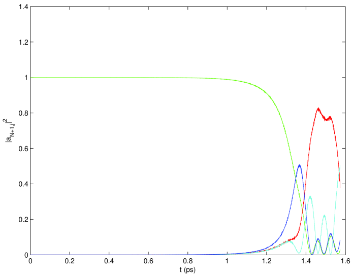
Figure 1: The excitation $|a_{N+1}|^{2}$ as a function of time in box 1 (green), box 2 (red), box3 (cyan) and box 4 (blue). Here N=14, and the effective masses, creating the funnel, were $\mu_{1}=1$, $\mu_{2}=1.02$, $\mu_{3}=1.04$, and $\mu_{4}=1.06$. All wall masses were M=100. The excitation reaches the last (4th) box directly from the first box, with 50% strength, at about 1.3 ps. The Förster term is not included.

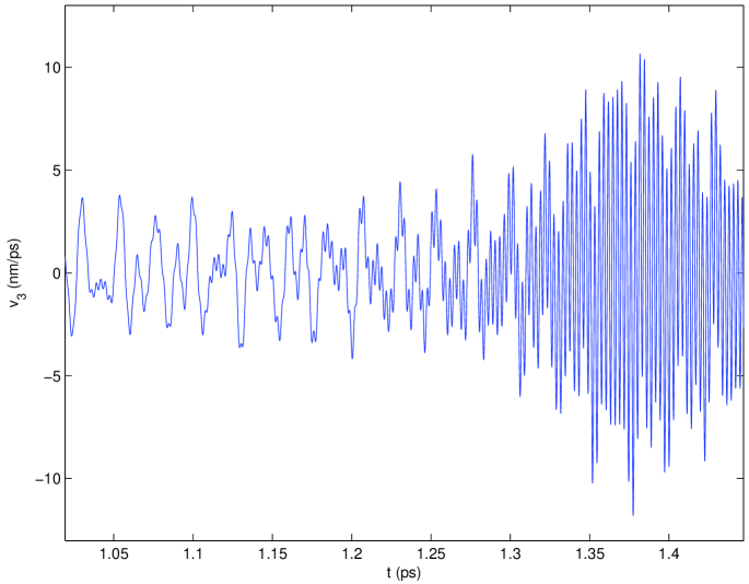
Figure 2: The velocity of the wall between box 3 and box 4 around the time of the transparency instability shows the slow, low amplitude oscillations giving way to the fast, large amplitude oscillations driven by the growing fluctuating component of the Fermi pressure.

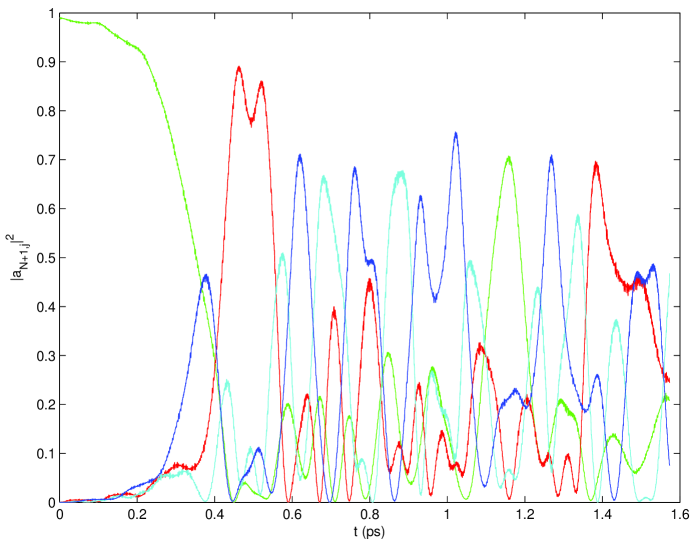
Figure 3: The excitation $|a_{N+1}|^{2}$ as a function of time, as in Fig. 1, but with a slight admixture of the ground state in box 1, so that the Fermi pressure fluctuations were already appreciable at t=0. The excitation now reaches the last (4th) box directly from the first box, with about 45% strength, in less than 400 fs. Transparency of the system is clear as the energy moves rapidly thereafter from box to box.

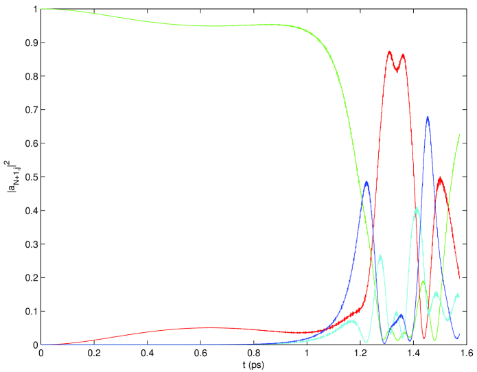
Figure 4: The excitation $|a_{N+1}|^{2}$ as a function of time in box 1 (green), box 2 (red), box3 (cyan) and box 4 (blue). Here N=14, and the effective masses, creating the funnel, were $\mu_{1}=1$, $\mu_{2}=1.02$, $\mu_{3}=1.04$, and $\mu_{4}=1.06$. All wall masses were M=100. The Förster term is included with a dimensionless coupling constant 0.04, as estimated in the text.

Figure 5: The excitation $|a_{N+1}|^{2}$ as a function of time in box 1 (green), box 2 (red), box3 (cyan) and box 4 (blue). As before, N=14, and the effective masses, creating the funnel, were $\mu_{1}=1$, $\mu_{2}=1.02$, $\mu_{3}=1.04$, and $\mu_{4}=1.06$. All wall masses were M=100. The Förster term is included with a dimensionless coupling constant 0.1, corresponding to a Förster transition time comparable to the time for Fermi pressure oscillations to develop. The initial transfer is now mainly to box 2, not box 4.

References

- (1) F. Fassioli, R. Dinshaw, P.C. Arpin, and G.D. Scholes (2014). Photosynthetic light harvesting: excitons and coherence. Journal of the Royal Society Interface, 11:20130901.
- (2) O.P. Ernst, D.T. Lodowski, M. Elstner, P. Hegemann, L.S. Brown, and H. Kandori (2014). Microbial and animal rhodopsins: Structures, functions, and molecular mechanisms. Chemical Reviews, 114:126-163.
- (3) G. S. Engel, T. R. Calhoun, and E. L. Read, T-K. Ahn, T. Mancal Y-C. Cheng, R. E. Blankenship, and G. R. Fleming (2007). Evidence for wavelike energy transfer through quantum coherence in photosynthetic systems. Nature, 446:782-786.
- (4) F. Fassioli, A. Olaya-Castro, and G.D. Scholes (2012). Coherent energy transfer under incoherent light conditions. J. Phys. Chem. Lett. 3:3136-3142.
- (5) Y-C. Cheng and G.R. Fleming (2009). Dynamics of Light Harvesting in Photosynthesis. Annu. Rev. Phys. Chem. 60:241-262.
- (6) L. Tarr (2005). Quantum Systems with Time-dependent Boundaries. http://solar.physics.montana.edu/tarrl/pubs/Lucas.Tarr.Reed.College.Thesis.pdf. (Reed College undergraduate thesis).
- (7) R. Phillips, J. Kondev, J. Theriot, and H. Garcia (2012). Physical Biology of the Cell. Garland Science, 2 edition.
- (8) T. Ritz, A. Damjanovic, and K. Schulten (2002). The Quantum Physics of Photosynthesis. ChemPhysChem, 3:243-248.