Abstract

We study collective excitations of cold (2+1)-dimensional fundamental matter living on a defect of the four-dimensional ${\cal N}=4$ super Yang-Mills theory in the Higgs branch. This system is realized holographically as a D3-D5 brane intersection, in which the D5-brane is treated as a probe with a non-zero gauge flux across the internal part of its worldvolume. We study the holographic zero sound mode in the collisionless regime at low temperature and find a simple analytic result for its dispersion relation. We also find the diffusion constant of the system in the hydrodynamic regime at higher temperature. In both cases we study the dependence on the flux parameter which determines the amount of Higgs symmetry breaking. We also discuss the anyonization of this construction.

1 Introduction

The gauge/gravity holographic duality has been recently employed to study compressible states of cold matter [1, 2, 3, 4]. In these studies the intersection of two different types of branes (D$p$ and D$q$ with $q\geq p$) is considered. The higher dimensional D$q$-branes are treated as probes in the gravitational background generated by the lower dimensional D$p$-branes. On the field theory side the probe branes add hypermultiplets in the fundamental representation of the gauge group [5]. These matter fields live generically in a defect of the unflavored theory. The probe approximation corresponds to the quenched approximation on the field theory side (see [6] for an unifying formalism of the different brane intersections and for a complete list of references).

In the brane setup the non-zero charge density needed to have a compressible state is generated by turning on a worldvolume gauge field [7]. The dominant collective excitation of these systems at sufficiently low temperatures is a sound mode (the holographic zero sound [1]). At enough high temperature thermal effects dominate over quantum effects and the system enters in a hydrodynamic regime in which a diffusion mode dominates. These two regimes are connected by a collisionless/hydrodynamic crossover transition.

In this paper we will consider the intersection of D3- and D5-branes, according to the array:

$$\begin{array}[]{cccccccccccl}&0&1&2&3&4&5&6&7&8&9&\\ D3:&\times&\times&\times&\times&\_&\_&\_&\_&\_&\_&\\ D5:&\times&\times&\times&\_&\times&\times&\times&\_&\_&\_&\end{array}$$

This D3-D5 system is dual [8] to a defect theory in which ${\cal N}=4$, $d=4$ super Yang-Mills theory in the bulk is coupled to ${\cal N}=4$, $d=3$ fundamental hypermultiplets localized at the defect [9, 10]. We will restrict ourselves to the configuration in which the D3- and D5-branes are not separated in 789 directions, which corresponds to having massless hypermultiplet fields.

Turning on a flux of the worldvolume gauge field along the internal directions 456, one realizes the Higgs branch of the theory [11], in which some components of the fundamental hypermultiplets acquire a non-vanishing vacuum expectation value. The worldvolume flux induces a bending of the D5-brane along the 3 direction. As shown in [11] one can then regard the probe D5-brane as a bound state of D3-branes or, equivalently, one can interpret that some of the D3-branes end on a D5-brane and recombine with it. The (2+1)-dimensional defect induced by the D5-brane represents a domain wall separating two regions with gauge groups with different ranks (the jump in the rank as one crosses the wall is proportional to the worldvolume flux).

In this paper we study the collective behavior of cold matter confined to the defect, when the system is in the Higgs branch. The first step in our analysis will be determining the precise configuration of the probe which represents the system at non-zero chemical potential, temperature $T$, and magnetic field $B$ (the $T=B=0$ case was studied in [12]). We will then study the spectrum of excitations and we will determine the dispersion relation of the zero sound mode at $T=0$. We will find a simple analytical expression for the speed of zero sound as a function of the flux. Moreover, since the intersection is (2+1)-dimensional, we can consider mixed Dirichlet-Neumann boundary conditions in the UV, which corresponds to performing an alternative quantization [13] and thus the charge carriers become anyons. In the presence of the magnetic field the spectrum of the zero sound mode is generically gapped although, as in [6], one can adjust the anyon parameter to some critical value such that the resulting spectrum is gapless. We will also study the system at non-zero temperature and we will find the corresponding diffusion constant.

The rest of this paper is organized as follows. In section 2 we will determine precisely our brane configuration. The fluctuations of the D5-brane probe will be analyzed in section 3. In section 4 we obtain the spectrum of the zero sound. Section 5 is devoted to the calculation of the diffusion constant. Finally, in section 6 we summarize our results and discuss some extensions of our work.

2 The brane setup

Let us consider the supergravity solution corresponding to a stack of $N$ D3-branes at non-zero temperature. The corresponding near-horizon geometry is a black hole in $AdS_{5}\times{\mathbb{S}}^{5}$, whose metric is:

$$ds^{2}_{10}={r^{2}\over R^{2}}\Big{(}-fdt^{2}+d\vec{x}^{2}\Big{)}+{R^{2}\over r^{2}}\Big{(}{dr^{2}\over f}+r^{2}d\Omega_{5}^{2}\Big{)}\ ,$$ (2.1)

where $\vec{x}=(x,y,z)$, $R^{4}=4\pi g_{s}N\alpha^{\prime 2}$ is the $AdS_{5}$ radius and the blackening factor

$$f(r)\,=\,1\,-\,{r_{h}^{4}\over r^{4}}\,\,.$$ (2.2)

In (2.2) $r_{h}$ is the horizon radius, related to the black hole temperature $T$ as $r_{h}=\pi\,T$. The D3-brane background is endowed with a Ramond-Ramond five-form $F^{(5)}$, whose potential will be denoted by $C^{(4)}$. The component of $C^{(4)}$ along the Minkowski coordinates is given by:

$$\Big{[}\,C^{(4)}\,\Big{]}_{t,\vec{x}}\,=\,{r^{4}\over R^{4}}\,\,.$$ (2.3)

Let us now embed a D5-brane probe in the geometry (2.1) in such a way that it is extended along $(x,y,r)$ and wraps a maximal ${\mathbb{S}}^{2}\subset{\mathbb{S}}^{5}$ (parameterized by two angles $\theta$ and $\varphi$). If the D5-brane is bent along the third Cartesian coordinate $z=z(r)$, the induced metric on the worldvolume of the D5-brane is:

$$ds_{6}^{2}\,=\,r^{2}[\,-f\,dt^{2}\,+\,dx^{2}+dy^{2}]\,+\,\Big{[}{1\over r^{2}\,f}+r^{2}\,z^{\prime 2}\,\Big{]}\,dr^{2}\,+\,d\theta^{2}+\sin^{2}\theta\,d\varphi^{2}\,\,,$$ (2.4)

where we have taken units in which the $AdS_{5}$ radius $R=1$. We switch on a worldvolume gauge field given by:

$$F\,=\,A_{t}^{\prime}\,dr\wedge dt\,+\,B\,dx\wedge dy+\,q\sin\theta\,d\theta\wedge d\varphi\,\,,$$ (2.5)

with $q$ being a constant (the amount of flux). As usual, the $r\,t$ component of $F$ in (2.5) is required in order to have a non-vanishing charge density. The action of a D5-brane probe in the background geometry is given by the sum of the Dirac-Born-Infeld (DBI) and Wess-Zumino (WZ) terms:

$$S_{D5}\,=\,-\,T_{5}\,\int d^{6}\xi\,\sqrt{-\det(g+F)}\,+\,T_{5}\,\int d^{6}\xi\,\,\,\hat{C}^{(4)}\,\wedge F\,\,,$$ (2.6)

where $T_{5}$ is the tension of the D5-brane and $g$ is the induced metric on the worldvolume. The DBI determinant for our ansatz is:

$$\sqrt{-\det(g+F)}\,=\,\sqrt{r^{4}+B^{2}}\,\sqrt{1+r^{4}\,f\,z^{\prime 2}\,-\,A_{t}^{\prime\,2}}\,\sqrt{1+q^{2}}\,\sin\theta\,\,,$$ (2.7)

while the WZ Lagrangian density is given by:

$${\cal L}_{WZ}\,=\,T_{5}\,\hat{C}_{4}\,\wedge\,F\,=\,T_{5}\,q\,r^{4}\,z^{\prime}\,\sin\theta\,dt\wedge dx\wedge dy\wedge dr\wedge d\theta\wedge d\varphi\,\,.$$ (2.8)

Therefore, after integrating over the angular variables, the total Lagrangian density becomes:

$${\cal L}\,=\,4\pi T_{5}\,\Big{[}-\sqrt{r^{4}+B^{2}}\,\sqrt{1+r^{4}\,f\,z^{\prime 2}\,-\,A_{t}^{\prime 2}}\,\sqrt{1+q^{2}}+q\,r^{4}\,z^{\prime}\Big{]}\,\,,$$ (2.9)

The equation of motion for $A_{t}$ leads to:

$${\sqrt{r^{4}+B^{2}}\,A_{t}^{\prime}\over\sqrt{1+r^{4}\,f\,z^{\prime 2}\,-\,A_{t}^{\prime 2}}}\,\sqrt{1+q^{2}}\,=\,d\,\,,$$ (2.10)

where $d$ is a constant proportional to the charge density. From this equation we get $A_{t}^{\prime}$ as a function of $z^{\prime}$:

$$A_{t}^{\prime}\,=\,{d\,\sqrt{1+r^{4}\,f\,z^{\prime 2}}\over\sqrt{d^{2}+(1+q^{2})\,(r^{4}+B^{2})}}\,\,.$$ (2.11)

The equation of motion for $z$ leads to the equation:

$$-\sqrt{r^{4}+B^{2}}\,{r^{4}\,f\,z^{\prime}\over\sqrt{1+r^{4}\,f\,z^{\prime 2}\,-\,A_{t}^{\prime\,2}}}\,\sqrt{1+q^{2}}\,+\,q\,r^{4}\,=\,c_{z}\,\,,$$ (2.12)

where $c_{z}$ is a constant of integration. By imposing regularity at the horizon of the embedding function $z(r)$ [14], yields $c_{z}\,=\,q\,r_{h}^{4}$. It is then possible to use (2.11) and (2.12) to obtain $A_{t}^{\prime}$ and $z^{\prime}$ as functions of the coordinate $r$:

$$A_{t}^{\prime}\,=\,{d\over\sqrt{r^{4}+d^{2}+q^{2}\,r_{h}^{4}+(1+q^{2})\,B^{2}}}\,\,,\qquad\qquad z^{\prime}\,=\,{q\over\sqrt{r^{4}+d^{2}+q^{2}\,r_{h}^{4}+(1+q^{2})\,B^{2}}}\,\,.\qquad$$ (2.13)

In what follows it is convenient to express the different results in terms of the chemical potential $\mu$ at $T=B=0$, which is given by:

$$\mu=A_{t}(r=\infty)=\int_{0}^{\infty}\,dr\,A_{t}^{\prime}(r){\big{|}_{T=B=0}}={4\,\Gamma\big{(}{5\over 4}\big{)}^{2}\over\sqrt{\pi}}\,d^{{1\over 2}}\,\,.$$ (2.14)

3 Fluctuations

Let us allow fluctuations of the gauge field along the Minkowski directions of the intersection, in the form:

$$A\,=\,A^{(0)}\,+\,a(r,x^{\mu})\,\,,$$ (3.1)

where $A^{(0)}$ is the gauge potential for the field strength (2.5) and $a(r,x^{\mu})=a_{\nu}(r,x^{\mu})\,dx^{\nu}$ is a fluctuation. The total gauge field strength is:

$$F_{ab}\,=\,F^{(0)}_{ab}\,+\,f_{ab}\,\,,$$ (3.2)

with $F^{(0)}=dA^{(0)}$ is the two-form written in (2.5). In order to write the Lagrangian for the fluctuations at second order, let us split the inverse of the matrix $g^{(0)}\,+\,F^{(0)}$ as:

$$\Big{(}\,g^{(0)}\,+\,F^{(0)}\Big{)}^{-1}\,=\,{\cal G}^{-1}\,+\,{\cal J}\,\,,$$ (3.3)

where ${\cal G}^{-1}$ is the symmetric part and ${\cal J}$ is the antisymmetric part (${\cal G}$ is the so-called open string metric). Then, the Lagrangian density for the fluctuations is:

$${\cal L}\,\sim\,{r^{4}+B^{2}\over\sqrt{r^{4}+d^{2}+q^{2}\,r_{h}^{4}+(1+q^{2})\,B^{2}}}\,\,\,\,\Big{(}\,{\cal G}^{ac}\,{\cal G}^{bd}\,-\,{\cal J}^{ac}\,{\cal J}^{bd}\,+\,{1\over 2}\,{\cal J}^{cd}\,{\cal J}^{ab}\Big{)}f_{cd}\,f_{ab}\,\,,$$ (3.4)

where the Latin indices take values in $a,b,c\in\{t,x,y,r\}$. Notice that we are choosing a gauge in which $a_{r}=0$. The equation of motion for $a^{d}$ derived from (3.4) is:

$$\partial_{c}\,\Bigg{[}{r^{4}+B^{2}\over\sqrt{r^{4}+d^{2}+q^{2}\,r_{h}^{4}+(1+q^{2})\,B^{2}}}\,\Big{(}\,{\cal G}^{ca}\,{\cal G}^{db}\,-\,{\cal J}^{ca}\,{\cal J}^{db}\,+\,{1\over 2}\,{\cal J}^{cd}\,{\cal J}^{ab}\Big{)}\,f_{ab}\Bigg{]}\,=\,0\,\,.$$ (3.5)

Let us write these equations in the case in which the fluctuation fields $a_{\nu}$ only depend on the coordinates $r$, $t$, and $x$. We first Fourier transform the gauge field to momentum space as:

$$a_{\nu}(r,t,x)\,=\,\int{d\omega\,dk\over(2\pi)^{2}}\,a_{\nu}(r,\omega,k)\,e^{-i\omega t+ikx}\,\,.$$ (3.6)

In what follows it will be understood that the gauge field is written in momentum space. Moreover, we define the electric field $E$ as the gauge-invariant combination:

$$E\,=\,k\,a_{t}\,+\,\omega\,a_{x}\,\,.$$ (3.7)

The equations of motion reduce to a set of two coupled equations for $E$ and the transverse gauge field fluctuation $a_{y}$. The equation for the fluctuation of the electric field $E$ is given by:

$$E^{\prime\prime}+\,\partial_{r}\log\Bigg{[}{r^{4}f\over r^{4}+B^{2}}\,{\sqrt{r^{4}+d^{2}+q^{2}\,r_{h}^{4}+(1+q^{2})\,B^{2}}\,\Big{(}d^{2}+(1+q^{2})\,(r^{4}+B^{2})\Big{)}\over(1+q^{2})(\omega^{2}-\,f\,k^{2})r^{4}+[(1+q^{2})\,B^{2}\,+\,d^{2}]\,\omega^{2}}\Bigg{]}\,E^{\prime}$$

$$\qquad\qquad+{1\over r^{4}f^{2}}\,{(1+q^{2})(\omega^{2}-\,f\,k^{2})r^{4}+[(1+q^{2})\,B^{2}\,+\,d^{2}]\,\omega^{2}\over r^{4}+d^{2}+q^{2}\,r_{h}^{4}+(1+q^{2})\,B^{2}}\,E$$

$$=-{4iBd\over r\,(r^{4}+B^{2})f}\,{(1+q^{2})(\omega^{2}-\,f\,k^{2})r^{4}+[(1+q^{2})\,B^{2}\,+\,d^{2}]\,\omega^{2}\over\sqrt{r^{4}+d^{2}+q^{2}\,r_{h}^{4}+(1+q^{2})\,B^{2}}\,\Big{(}d^{2}+(1+q^{2})\,(r^{4}+B^{2})\Big{)}}\,a_{y}\,\,.$$ (3.8)

The equation for the transverse fluctuation is:

$$a_{y}^{\prime\prime}\,+\,\partial_{r}\log\Bigg{[}{r^{4}\,f\over r^{4}+B^{2}}\,\sqrt{r^{4}+d^{2}+q^{2}\,r_{h}^{4}+(1+q^{2})\,B^{2}}\Bigg{]}\,a_{y}^{\prime}$$

$$\qquad\qquad+{1\over r^{4}f^{2}}\,{(1+q^{2})(\omega^{2}-\,f\,k^{2})r^{4}+[(1+q^{2})\,B^{2}\,+\,d^{2}]\,\omega^{2}\over r^{4}+d^{2}+q^{2}\,r_{h}^{4}+(1+q^{2})\,B^{2}}\,a_{y}$$

$$\qquad\qquad=\,{4iBd\over r\,(r^{4}+B^{2})f}\,{E\over\sqrt{r^{4}+d^{2}+q^{2}\,r_{h}^{4}+(1+q^{2})\,B^{2}}}\,\,.$$ (3.9)

Let us now see how one can eliminate the dependence of $r_{h}$ on the equations of motion by performing appropriate rescalings. First of all, we define a new radial variable $\hat{r}\,=\,r/r_{h}$. Then, one can check that $r_{h}$ is eliminated from (3.8) and (3.9) by defining the new rescaled (hatted) quantities as:

$$\hat{\omega}\,=\,{\omega\over r_{h}}\,\,,\qquad\qquad\hat{k}\,=\,{k\over r_{h}}\,\,,\qquad\qquad\hat{d}\,=\,{d\over r_{h}^{2}}\,\,,\qquad\qquad\hat{B}\,=\,{B\over r_{h}^{2}}\ .$$ (3.10)

The resulting equations are obtained from (3.8) and (3.9) by taking $r_{h}=1$ and substituting all quantities by their hatted counterparts. Hatted variables are utilized in the numerical integration of eqs. (3.8) and (3.9).

4 Zero sound

Let us now study the system at zero temperature. First we study the equations of motion (3.8) and (3.9) near the Poincaré horizon $r=0$. Assuming that $B$ is small ($B\sim r^{4}$), the equations of $E$ and $a_{y}$ are given by the coupled system:

$$E^{\prime\prime}\,+\,{4\,B^{2}\over r(r^{4}+B^{2})}\,E^{\prime}\,+\,{\omega^{2}\over r^{4}}\,E = -\,{4i\,B\omega^{2}\over r(r^{4}+B^{2})}\,a_{y}$$

$$a_{y}^{\prime\prime}\,+\,{4\,B^{2}\over r(r^{4}+B^{2})}\,a_{y}^{\prime}\,+\,{\omega^{2}\over r^{4}}\,a_{y} = \,{4i\,B\over r(r^{4}+B^{2})}\,E\,\,.$$ (4.1)

This is the same system as in the D3-D5 case with zero flux of [4]. We can readily write its solution in matrix form as:

$$\begin{pmatrix}E\\ \\ a_{y}\end{pmatrix}\,=\,e^{{i\omega\over r}}\,\begin{pmatrix}r&&&\big{(}1-{i\omega\over r}\big{)}\,{B\over\omega}\\ {}&{}\\ {i\over\omega}\,\big{(}1-{i\omega\over r}\big{)}\,{B\over\omega}&&&{i\over\omega}\,r\end{pmatrix}\,\begin{pmatrix}c_{1}\\ \\ c_{2}\end{pmatrix}\,\,,$$ (4.2)

where $c_{1}$ and $c_{2}$ are integration constants and we have imposed infalling boundary conditions at the horizon. Next we take the limit of low frequency and momentum in such a way that $\omega\sim k\sim{\cal O}(\epsilon)$. For small $\omega$ the solution (4.2) can be written as:

$$\begin{pmatrix}E\\ \\ a_{y}\end{pmatrix}\,=\,\begin{pmatrix}r+i\omega&&&\,{B\over\omega}\,{}&{}\\ \\ {iB\over\omega^{2}}&&&{i\over\omega}\,(r+i\omega)\end{pmatrix}\,\begin{pmatrix}c_{1}\\ \\ c_{2}\end{pmatrix}\,\,.$$ (4.3)

We now take the low frequency limit first. One can verify that the equations decouple in this limit. Actually, the equation for $E$ becomes:

$$E^{\prime\prime}+\partial_{r}\log{\sqrt{r^{4}+d^{2}}\,[d^{2}+(1+q^{2})\,r^{4}]\over(1+q^{2})(\omega^{2}-\,k^{2})r^{4}+\omega^{2}\,d^{2}}\,E^{\prime}\,=\,0\,\,.$$ (4.4)

This equation can be readily integrated as:

$$E(r)\,=\,E^{(0)}\,-\,c_{E}\,\int_{r}^{\infty}\,d\rho\,{(1+q^{2})(\omega^{2}-\,k^{2})\rho^{4}+\omega^{2}\,d^{2}\over\sqrt{\rho^{4}+d^{2}}\,[d^{2}+(1+q^{2})\,\rho^{4}]}\,\,,$$ (4.5)

where $E^{(0)}=E(r\to\infty)$. Actually, if we define the integrals:

$${\cal K}_{1}(r)\,=\,\int_{r}^{\infty}\,{\rho^{4}\over\sqrt{\rho^{4}+d^{2}}\,[d^{2}+(1+q^{2})\,\rho^{4}]}\,\,d\rho$$

$${\cal K}_{2}(r)\,=\,\int_{r}^{\infty}\,{d\rho\over\sqrt{\rho^{4}+d^{2}}\,[d^{2}+(1+q^{2})\,\rho^{4}]}\,\,,$$ (4.6)

then, $E(r)$ can be written as:

$$E(r)\,=\,E^{(0)}\,-\,c_{E}\,\Big{[}(1+q^{2})(\omega^{2}-\,k^{2})\,{\cal K}_{1}(r)\,+\,\omega^{2}\,d^{2}\,{\cal K}_{2}(r)\Big{]}\,\,.$$ (4.7)

Let us now expand this result near the horizon. We first expand the integrals ${\cal K}_{1}(r)$ and ${\cal K}_{2}(r)$ near $r=0$ as:

$${\cal K}_{1}(r)\,=\,\bar{\cal K}_{1}\,+\,{\mathcal{O}}(r^{2})\,\,,\qquad\qquad{\cal K}_{2}(r)\,=\,\bar{\cal K}_{2}\,-{r\over d^{3}}\,+\,{\mathcal{O}}(r^{2})\,\,,$$ (4.8)

where $\bar{\cal K}_{1}={\cal K}_{1}(r=0)$ and $\bar{\cal K}_{2}={\cal K}_{2}(r=0)$. It is interesting to notice that the quantities $\bar{\cal K}_{1}$ and $\bar{\cal K}_{2}$ are not independent. Indeed, they satisfy the relation:

$$(1+q^{2})\bar{\cal K}_{1}\,+\,d^{2}\,\bar{\cal K}_{2}\,=\,\int_{0}^{\infty}{d\rho\over\sqrt{\rho^{4}+d^{2}}}\,=\,{\mu\over d}\,\,.$$ (4.9)

Moreover, if we define the flux function ${\cal F}(q)$ as:

$${\cal F}(q)\,\equiv\,{2d\over\mu}\,(1+q^{2})\,\bar{\cal K}_{1}=(1+q^{2})\,F\Big{(}1,{5\over 4};{3\over 2};-q^{2}\Big{)}\ ,$$ (4.10)

then, near $r=0$ we can write $E(r)$ as:

$$E\,=\,c_{E}\,{\omega^{2}\over d}\,r\,+\,E^{(0)}\,-\,{c_{E}\over d}\,\Big{[}\mu\,\omega^{2}\,-\,{\mu\over 2}\,{\cal F}(q)\,k^{2}\Big{]}\,\,.$$ (4.11)

It is worth stressing that the whole effect of the flux in (4.11) is equivalent to multiplying $k^{2}$ by the flux function ${\cal F}(q)$.

The equation for $a_{y}$ for low frequency is:

$$a_{y}^{\prime\prime}\,+\,\partial_{r}\,\log\Big{(}r^{4}+d^{2}\Big{)}^{{1\over 2}}\,a_{y}^{\prime}=0\,\,.$$ (4.12)

This equation can be integrated twice to give:

$$a_{y}(r)\,=\,a_{y}^{(0)}\,-\,c_{y}\int_{r}^{\infty}\,{d\rho\over(\rho^{4}+d^{2})^{{1\over 2}}}\,=\,a_{y}^{(0)}\,-\,{c_{y}\over r}\,F\Big{(}\,{1\over 2},{1\over 4};{5\over 4};-{d^{2}\over r^{4}}\,\Big{)}\ \,\,,$$ (4.13)

with $a_{y}^{(0)}\,=\,a_{y}(r\to\infty)$. For small $r$ the previous solution becomes:

$$a_{y}(r)\,\approx\,a_{y}^{(0)}\,-\,c_{y}\,{\mu\over d}\,+\,c_{y}\,{r\over d}\,\,.$$ (4.14)

Let us now match the two expressions we have found for $E$ and $a_{y}$ in this double low frequency and near-horizon limit (eqs. (4.3), (4.11), and (4.14)). Looking at the terms linear in $r$ we get find relations between the constants $c_{1}$, $c_{2}$, $c_{E}$, and $c_{y}$:

$$c_{1}\,=\,{\omega^{2}\over d}\,c_{E}\,\,,\qquad\qquad\qquad c_{2}\,=\,-i{\omega\over d}\,c_{y}\,\,.$$ (4.15)

The identification of the constant terms yields the following matrix relation

$$\begin{pmatrix}E^{(0)}\\ \\ a_{y}^{(0)}\end{pmatrix}\,=\,\begin{pmatrix}i{\omega^{3}\over d}\,+\,{\mu\over d}\,\omega^{2}\,-\,{\mu\over 2d}\,{\cal F}(q)\,k^{2}&&&-i{B\over d}\\ {}&{}\\ {iB\over d}&&&{i\omega\over d}\,+\,{\mu\over d}\end{pmatrix}\,\begin{pmatrix}c_{E}\\ \\ c_{y}\end{pmatrix}\,\,.$$ (4.16)

Let us now require that our fluctuation modes satisfy the following mixed Dirichlet-Neumann boundary conditions at the UV[15, 16]:

$$\lim_{r\to\infty}\,\Big{[}\,n\,r^{\,2}\,f_{r\,\mu}\,-\,{1\over 2}\,\epsilon_{\mu\alpha\beta}\,f^{\alpha\beta}\,\big{]}\,=\,0\,\,,$$ (4.17)

with $n$ being some constant (the Dirichlet boundary conditions correspond to taking $n=0$). As in the case with $q=0$, these conditions are equivalent to:

$$\lim_{r\to\infty}\,E\,=\,-i\,n\,\lim_{r\to\infty}\,\big{[}\,r^{\,2}\,a_{y}^{\prime}\,\big{]}\,\,,\qquad\qquad\qquad\lim_{r\to\infty}\,a_{y}\,=\,i\,{n\over\omega^{2}-k^{2}}\,\lim_{r\to\infty}\,\big{[}\,r^{\,2}\,E^{\prime}\,\big{]}\,\,.$$ (4.18)

The quantities on the left-hand-side of (4.18) are the UV values $E^{(0)}$ and $a_{y}^{(0)}$. In order to obtain the values of the right-hand-side of the two conditions in (4.18), notice that the radial derivatives of $E$ and $a_{y}$ can be obtained from their low-frequency values (4.5) and (4.13):

$${\partial E\over\partial r}\,\Big{|}_{r\to\infty}\approx(\omega^{2}-k^{2})\,c_{E}\,r^{-2}\,\,,\qquad\qquad{\partial a_{y}\over\partial r}\,\Big{|}_{r\to\infty}\approx c_{y}\,r^{-2}\,\,.$$ (4.19)

From these expressions we can recast the boundary conditions (4.17) as relations between the constants $E^{(0)}$, $a_{y}^{(0)}$, $c_{E}$, and $c_{y}$. Indeed, let us define $E_{n}^{(0)}$ and $a_{y,n}^{(0)}$ as:

$$E_{n}^{(0)}\,\equiv E^{(0)}\,+\,i\,n\,c_{y}\,\,,\qquad\qquad a_{y,n}^{(0)}\,=\,a_{y}^{(0)}\,-\,i\,n\,c_{E}\,\,.$$ (4.20)

Then, (4.18) is equivalent to the conditions:

$$E_{n}^{(0)}\,=\,a_{y,n}^{(0)}\,=\,0\,\,.$$ (4.21)

Moreover, combining (4.16) and (4.20) we conclude that $E_{n}^{(0)}$ and $a_{y,n}^{(0)}$ are related to the constants $c_{E}$ and $c_{y}$ by the following matrix equation:

$$\begin{pmatrix}E_{n}^{(0)}\\ \\ a_{y,n}^{(0)}\end{pmatrix}\,=\,\begin{pmatrix}i{\omega^{3}\over d}\,+\,{\mu\over d}\,\omega^{2}\,-\,{\mu\over 2d}\,{\cal F}(q)\,k^{2}&&&-i{B\over d}+in\\ {}&{}\\ {iB\over d}-in&&&{i\omega\over d}\,+\,{\mu\over d}\end{pmatrix}\,\begin{pmatrix}c_{E}\\ \\ c_{y}\end{pmatrix}\,\,.$$ (4.22)

Furthermore, the non-trivial fulfillment of the condition (4.21) is equivalent to the vanishing of the determinant of the matrix in (4.22), which determines the dispersion relation satisfied by $\omega$ and $k$ for the zero sound modes:

$$\omega^{4}\,-\,2i\mu\,\omega^{3}\,+\,i\,{\mu\over 2}\,{\cal F}(q)\,\omega\,k^{2}\,-\,\mu^{2}\,\omega^{2}\,+\,{\mu^{2}\over 2}\,{\cal F}(q)\,k^{2}\,+\,(B-nd)^{2}\,=\,0\,\,.$$ (4.23)

Notice that the effect of the flux in (4.23) is encoded in the substitution $k^{2}\to{\cal F}(q)\,k^{2}$. Let us now solve (4.23) for $\omega$ as a function of $k$ for small values of $(\omega,k)$. At leading order $\omega$ is real and given by:

$$\omega^{2}\,=\,{1+q^{2}\over 2}\,F\Big{(}1,{5\over 4};{3\over 2};-q^{2}\Big{)}\,\,k^{2}\,+\,{(B-nd)^{2}\over\mu^{2}}\,\,.$$ (4.24)

It follows from the last term in (4.24) that the spectrum is generically gapped for non-vanishing $B$ and $n$. However, it can be made gapless by adjusting the alternative quantization parameter $n$ to the critical value $n_{crit}=B/d$. This fact is illustrated in Fig. 1, where we compare the numerical results to our analytic formula (4.24). Moreover, from the coefficient of the momentum in the right-hand side of (4.24) we can extract the dependence of the speed of zero sound $u_{0}$ on the flux $q$. Indeed, by analyzing the behavior of the flux function (4.10), it is easy to conclude that $u_{0}=\pm 1/\sqrt{2}$ when $q=0$, whereas it approaches the maximal possible value $u_{0}=\pm 1$ as $q\to\infty$. Moreover, solving (4.23) for $\omega$ at next-to-leading order, we find the attenuation of the zero sound:

$${\rm Im}\,\omega\,=\,-{1\over\mu}\,\Big{[}{1+q^{2}\over 4}\,F\Big{(}1,{5\over 4};{3\over 2};-q^{2}\Big{)}\,\,k^{2}\,+\,{(B-nd)^{2}\over\mu^{2}}\Big{]}\,\,.$$ (4.25)

In Fig. 2 we compare the analytic results ${\rm Re}\,\omega$ and ${\rm Im}\,\omega$ with the numerics with varying flux $q$ and find very good agreement.

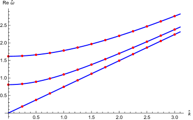
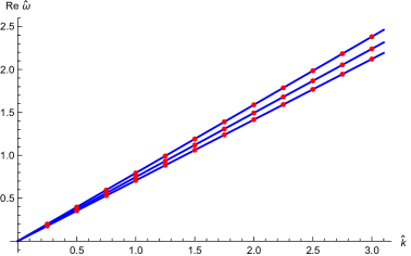
Figure 1: (left) The dispersions for the anyon fluid as the effective magnetic field is decreased to zero. The red points are the numerical values for $q=1$ and $n=0,n_{crit}/2,n_{crit}$ (top-down). (right) The dispersions for the anyon fluid at criticality $n=n_{crit}$ with increasing flux $q=0,1,2$ (bottom-up). Both figures are done at $\hat{d}=10^{6}$, $\hat{B}=3\cdot 10^{3}$.

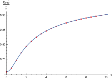
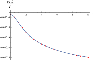
Figure 2: We display the dispersions of the lowest quasinormal mode at low temperature (zero sound) as functions of flux $q$. The analytic formulas (4.24) and (4.25) (blue curves) match extremely well with numerics (red points) for the real and imaginary parts of the frequency $\hat{\omega}$, respectively, as long as the temperature is kept small enough; we use $\hat{d}=10^{6}$ and $\hat{k}=10$ with $\hat{B}=\,n\,=0$.

5 Diffusion constant

Let us now consider the fluxed D3-D5 system at non-zero temperature. First, we analyze the equations of the fluctuations near the horizon $r=r_{h}$. It is easy to verify that the equations decouple in this limit and that the equation for $E$ near $r=r_{h}$ takes the form:

$$E^{\prime\prime}\,+\,\Big{(}{1\over r-r_{h}}\,+\,c_{1}\Big{)}\,E^{\prime}\,+\,\Big{(}{A\over(r-r_{h})^{2}}\,+\,{c_{2}\over r-r_{h}}\Big{)}\,E\,=\,0\,\,,$$ (5.1)

where $r_{h}$, $A$, $c_{1}$, and $c_{2}$ are constants. Equation (5.1) can then be solved in a Frobenius series around $r=r_{h}$. After this near-horizon expansion we perform a low frequency expansion by considering $k\sim{\mathcal{O}}(\epsilon)$, $\omega\sim{\cal O}(\epsilon^{2})$. The coefficients $A$, $c_{1}$, and $c_{2}$ at leading order in $\epsilon$ are:

$$A\,=\,{\omega^{2}\over 16\,r_{h}^{2}}$$

$$c_{1}\,=\,4(1+q^{2})\,{r_{h}^{3}\over d^{2}+(1+q^{2})(r_{h}^{4}+B^{2})}\,{k^{2}\over\omega^{2}}\,+\,\ldots$$

$$c_{2}\,=\,-{1+q^{2}\over 4}\,{r_{h}\over d^{2}+(1+q^{2})(r_{h}^{4}+B^{2})}\,\,k^{2}\,+\,\ldots\,\,.$$ (5.2)

It can be checked that near $r=r_{h}$, at leading order in $\epsilon$, the electric field $E(r)$ can be approximated as:

$$E\approx\,E_{nh}\,\big{[}1\,+\,\beta(r-r_{h})\,\big{]}\,\,,$$ (5.3)

where $E_{nh}$ is the value of $E$ at the horizon and $\beta$ is a constant coefficient given by:

$$\beta\,=\,i\,{k^{2}\over\omega}\,(1+q^{2})\,{r_{h}^{2}\over d^{2}+(1+q^{2})\,(r_{h}^{4}+B^{2})}\,\,.$$ (5.4)

We now perform the limits in opposite order. For low frequency, the equation of motion for $E$ can be written as:

$$E^{\prime\prime}\,-\,\partial_{r}\,\log\Bigg{[}{r^{4}+B^{2}\over\sqrt{r^{4}+d^{2}+q^{2}\,r_{h}^{4}+(1+q^{2})\,B^{2}}\,\Big{(}d^{2}+(1+q^{2})\,(r^{4}+B^{2})\Big{)}}\Bigg{]}\,E^{\prime}\,=\,0\,\,.$$ (5.5)

This equation can be integrated as:

$$E(r)\,=\,E^{(0)}+c_{E}\,{\cal I}(r)\,\,,$$ (5.6)

where $E^{(0)}$ is the UV value of $E$, $c_{E}$ is an integration constant, and ${\cal I}(r)$ is the integral:

$${\cal I}(r)\,=\,\int_{r}^{\infty}\,d\rho\,{\rho^{4}+B^{2}\over\sqrt{\rho^{4}+d^{2}+q^{2}\,r_{h}^{4}+(1+q^{2})\,B^{2}}\,\Big{(}d^{2}+(1+q^{2})\,(\rho^{4}+B^{2})\Big{)}}\,\,.$$ (5.7)

We now expand $E(r)$ in (5.6) near the horizon:

$$E(r)\,=\,E^{(0)}+c_{E}\,{\cal I}(r_{h})\,-\,{(r_{h}^{4}+B^{2})\,c_{E}\over\big{[}d^{2}+(1+q^{2})\,(r_{h}^{4}+B^{2})\big{]}^{{3\over 2}}}\,\,(r-r_{h})\,+\,\ldots\,\,.$$ (5.8)

Let us now compare (5.3) and (5.8). From the comparison of the constant terms we arrive at:

$$E^{(0)}\,=\,E_{nh}-c_{E}\,{\cal I}(r_{h})\,\,,$$ (5.9)

while matching the linear terms yields:

$$c_{E}\,=\,-\,\beta\,{\big{[}d^{2}+(1+q^{2})\,(r_{h}^{4}+B^{2})\big{]}^{{3\over 2}}\over r_{h}^{4}+B^{2}}\,E_{nh}\,=\,-i\,{k^{2}\over\omega}\,(1+q^{2}){r_{h}^{2}\over r_{h}^{4}+B^{2}}\,\big{[}d^{2}+(1+q^{2})\,(r_{h}^{4}+B^{2})\big{]}^{{1\over 2}}\,E_{nh}\,\,.$$ (5.10)

Thus, we can write $E^{(0)}$ as:

$$E^{(0)}\,=\,E_{nh}\,\Big{[}1+i\,{k^{2}\over\omega}\,{(1+q^{2})\,r_{h}^{2}\over r_{h}^{4}\,+\,B^{2}}\,\big{[}d^{2}+(r_{h}^{4}+B^{2})\,(1+q^{2})\big{]}^{{1\over 2}}{\cal I}(r_{h})\Big{]}\,\,.$$ (5.11)

From the condition $E^{(0)}=0$ we get a dispersion relation of the type $\omega=-iDk^{2}$, with the diffusion constant $D$:

$$D\,=\,(1+q^{2})\,{r_{h}^{2}\over r_{h}^{4}\,+\,B^{2}}\,\sqrt{d^{2}+(r_{h}^{4}+B^{2})\,(1+q^{2})}\,\,\,{\cal I}(r_{h})\,\,.$$ (5.12)

In terms of the hatted variables defined in (3.10), the diffusive dispersion relation can be written as:

$$\hat{\omega}\,=\,-i\,\hat{D}\,\hat{k}^{2}\,\,,$$ (5.13)

with the rescaled diffusion constant $\hat{D}$ defined as $\hat{D}\,=\,r_{h}\,D\,=\,\pi\,T\,D$. It is immediate from (5.12) to get the value of $\hat{D}$:

$$\hat{D}\,=\,(1+q^{2})\,{\sqrt{\hat{d}^{\,2}+(1+\hat{B}^{\,2})(1+q^{\,2})}\over 1+\hat{B}^{\,2}}\,\,{\cal J}(\hat{d},\hat{B},q)\,\,,$$ (5.14)

where ${\cal J}(\hat{d},\hat{B},q)$ is the integral

$${\cal J}(\hat{d},\hat{B},q)\,=\,\int_{1}^{\infty}\,dx\,{x^{4}+\hat{B}^{\,2}\over\sqrt{x^{4}+\hat{d}^{\,2}+q^{\,2}+(1+q^{\,2})\,\hat{B}^{\,2}}\,\,\big{[}\hat{d}^{\,2}+(x^{4}+\hat{B}^{\,2})(1+q^{\,2})\big{]}}\,\,.$$ (5.15)

In Fig. 3 we compare the numerical and analytical results for $\hat{D}$ as a function of $q$ for different values of the magnetic field $\hat{B}$.

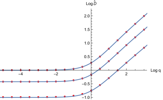
Figure 3: The numerical results (red points) for the diffusion constant $\hat{D}$ as a function of internal flux $q$ follow the analytic results (5.14) (plotted in blue curves) spot on. The different curves correspond to varying magnetic field strength $\hat{B}=0,1,2$ (top-down) with $\hat{d}=10^{6}$.

Let us study some limits of the formulas for the diffusion constant we have just found. First of all, it is interesting to point out that the integral ${\cal J}$ can be performed analytically when $\hat{d}=0$. The resulting expression for $\hat{D}$ is:

$$\hat{D}(\hat{d}=0)\,=\,\sqrt{{1+q^{2}\over 1+\hat{B}^{2}}}\,F\Big{(}{1\over 2},{1\over 4};{5\over 4};-q^{2}-(1+q^{2})\,\hat{B}^{2}\Big{)}\,\,.$$ (5.16)

As $\hat{d}\to 0$ when $T\to\infty$, the high temperature limit readily follows from (5.16):

$$\lim_{T\to\infty}\,\hat{D}\,=\,\sqrt{1+q^{2}}\,\,F\big{(}{1\over 2},{1\over 4};{5\over 4};-q^{2}\big{)}\,\,.$$ (5.17)

Thus, at large $T$ the diffusion constant behaves as:

$$D\,\approx{\sqrt{1+q^{2}}\over\pi\,T}\,\,F\big{(}{1\over 2},{1\over 4};{5\over 4};-q^{2}\big{)}\ \,\,,\qquad\qquad T\to\infty\,\,.$$ (5.18)

Interestingly, this last expression coincides with the one found in [17]. One can also study the opposite limit $T\to 0$. We find:

$$D\,\approx{\mu\over 2}\,{(1+q^{2})\,(\pi T)^{2}\over(\pi T)^{4}+B^{2}}\,\Bigg{(}{d^{2}\over d^{2}+(1+q^{2})\,B^{2}}\Bigg{)}^{{3\over 4}}\,\Bigg{[}\,F\Big{(}1,{5\over 4};{3\over 2};-q^{2}\Big{)}\,+\,{2B^{2}\over d^{2}}\Bigg{]}\,\,,\qquad\qquad T\to 0\,\,.\qquad$$ (5.19)

6 Conclusions and outlook

In this paper we studied the collective excitations of cold holographic matter confined to a (2+1)-dimensional defect of $4d$ ${\cal N}=4$ super Yang-Mills theory in the Higgs branch. The string theory realization of the system is a D3-D5 intersection with flux on the worldvolume of the D5-brane. We found a simple analytic expression for the dispersion relation of the zero sound as a function of the flux (see eqs. (4.24) and (4.25)). The speed of zero sound and the attenuation grow monotonically as the flux increases. We also studied the diffusion constant at higher temperatures.

Our work can be naturally extended along several directions. We could study other observables of the fluxed D3-D5 system with general boundary conditions. Some of these observables are the AC and DC conductivities of the anyonic fluid, as well as its diffusion constant. Moreover, we could easily extend our results to the general D$p$-D$(p+2)$ intersections with flux.

A more ambitious project could be the study collective excitations of the Higgs symmetry breaking even in more general holographic setups. One of such systems could be the D3-D7 intersection with an instanton on the D7-brane worldvolume. The explicit expression of this instanton at zero temperature and non-zero density has been found in [12]. Moreover, it was argued in [18] that this setup realizes holographically the color-flavor locking phase of color superconductivity. The analysis of the collective excitations of this model is of obvious interest and we intend to address this problem in the near future.

Acknowledgments

We thank Raúl Arias, Yago Bea, and Javier Mas for discussions. N.J. is supported by the Academy of Finland grant no. 1268023. G. I. and A. V. R. are funded by the Spanish grant FPA2011-22594, by the Consolider-Ingenio 2010 Programme CPAN (CSD2007-00042), by Xunta de Galicia (GRC2013-024), and by FEDER. We thank the Galileo Galilei Institute for Theoretical Physics for the hospitality and the INFN for partial support during the completion of this work.

References

- [1] A. Karch, D. T. Son and A. O. Starinets, “Zero Sound from Holography,” arXiv:0806.3796 [hep-th];“Holographic Quantum Liquid,” Phys. Rev. Lett. 102 (2009) 051602.
- [2] M. Kulaxizi and A. Parnachev, “Comments on Fermi Liquid from Holography,” Phys. Rev. D 78 (2008) 086004 [arXiv:0808.3953 [hep-th]]; “Holographic Responses of Fermion Matter,” Nucl. Phys. B 815, 125 (2009) [arXiv:0811.2262 [hep-th]].
- [3] R. A. Davison and A. O. Starinets, “Holographic zero sound at finite temperature,” Phys. Rev. D 85 (2012) 026004 [arXiv:1109.6343 [hep-th]].
- [4] D. K. Brattan, R. A. Davison, S. A. Gentle and A. O’Bannon, “Collective Excitations of Holographic Quantum Liquids in a Magnetic Field,” JHEP 1211 (2012) 084 [arXiv:1209.0009 [hep-th]].
- [5] A. Karch and E. Katz, “Adding flavor to AdS / CFT,” JHEP 0206 (2002) 043 [hep-th/0205236].
- [6] N. Jokela and A. V. Ramallo, “Universal properties of cold holographic matter,” arXiv:1503.04327 [hep-th].
- [7] S. Kobayashi, D. Mateos, S. Matsuura, R. C. Myers and R. M. Thomson, “Holographic phase transitions at finite baryon density,” JHEP 0702 (2007) 016 [hep-th/0611099].
- [8] A. Karch and L. Randall, “Locally localized gravity,” JHEP 0105, 008 (2001) [hep-th/0011156]; “Open and closed string interpretation of SUSY CFT’s on branes with boundaries,” JHEP 0106, 063 (2001) [hep-th/0105132].
- [9] O. DeWolfe, D. Z. Freedman and H. Ooguri, “Holography and defect conformal field theories,” Phys. Rev. D 66 (2002) 025009 [hep-th/0111135].
- [10] J. Erdmenger, Z. Guralnik and I. Kirsch, “Four-dimensional superconformal theories with interacting boundaries or defects,” Phys. Rev. D 66 (2002) 025020 [hep-th/0203020].
- [11] D. Arean, A. V. Ramallo and D. Rodriguez-Gomez, “Mesons and Higgs branch in defect theories,” Phys. Lett. B 641 (2006) 393 [hep-th/0609010]; “Holographic flavor on the Higgs branch,” JHEP 0705 (2007) 044 [hep-th/0703094.
- [12] M. Ammon, K. Jensen, K. Y. Kim, J. N. Laia and A. O’Bannon, “Moduli Spaces of Cold Holographic Matter,” JHEP 1211 (2012) 055 [arXiv:1208.3197 [hep-th]].
- [13] E. Witten, “SL(2,Z) action on three-dimensional conformal field theories with Abelian symmetry,” In *Shifman, M. (ed.) et al.: From fields to strings, vol. 2* 1173-1200 [hep-th/0307041].
- [14] O. Bergman, N. Jokela, G. Lifschytz and M. Lippert, “Quantum Hall Effect in a Holographic Model,” JHEP 1010 (2010) 063 [arXiv:1003.4965 [hep-th]].
- [15] N. Jokela, G. Lifschytz and M. Lippert, “Holographic anyonic superfluidity,” JHEP 1310 (2013) 014 [arXiv:1307.6336 [hep-th]]; “Flowing holographic anyonic superfluid,” JHEP 1410 (2014) 21 [arXiv:1407.3794 [hep-th]].
- [16] D. K. Brattan and G. Lifschytz, “Holographic plasma and anyonic fluids,” JHEP 1402 (2014) 090 [arXiv:1310.2610 [hep-th]].
- [17] R. C. Myers and M. C. Wapler, “Transport Properties of Holographic Defects,” JHEP 0812 (2008) 115 [arXiv:0811.0480 [hep-th]].
- [18] H. Y. Chen, K. Hashimoto and S. Matsuura, “Towards a Holographic Model of Color-Flavor Locking Phase,” JHEP 1002 (2010) 104 [arXiv:0909.1296 [hep-th]].