Approximate hedging with constant proportional transaction costs in financial markets with jumps

Thai Nguyen University of Ulm and University of Economics Hochiminh city; Email: thaibopy@ueh.edu.vn; thai.nguyen@uni-ulm.de    Serguei Pergamenschchikov Laboratoire de Mathématiques Raphaël Salem, UMR 6085 CNRS-Université de Rouen, France and International Laboratory SSP & QF, Tomsk State University, Russia, email: serge.pergamenchtchikov@univ-rouen.fr.
Abstract

We study the problem of option replication under constant proportional transaction costs in models where stochastic volatility and jumps are combined to capture the market’s important features. Assuming some mild condition on the jump size distribution we show that transaction costs can be approximately compensated by applying the Leland adjusting volatility principle and the asymptotic property of the hedging error due to discrete readjustments is characterized. In particular, the jump risk can be approximately eliminated and the results established in continuous diffusion models are recovered. The study also confirms that for the case of constant trading cost rate, the approximate results established by Kabanov and Safarian [22] and by Pergamenschikov [37] are still valid in jump-diffusion models with deterministic volatility using the classical Leland parameter in [25].

Key words: transaction costs; Leland strategy; jump models; stochastic volatility; approximate hedging; limit theorem; super-hedging; quantile hedging

2010 MSC Classification: 91G20; 60G44;
JEL Classification: G11, G13

1 Introduction

Many suggested mathematical models for stock prices have been trying to capture important markets features, e.g. leptokurtic feature, volatility clustering effect, implied volatility smile. These market properties are tractable in stochastic volatility models. However, diffusion-based stochastic volatility models assume that the market volatility can fluctuate autonomously but can not change suddenly and as a result, they could not take into account sudden and unpredictable market changes. Hence, in more realistic settings (extensions of the famous Black-Scholes framework), the continuity assumption of stock price should be relaxed to account for sudden market shocks due to good or bad market news. These sudden events can arrive according to a Poisson process. The change in the asset price right after the market receives a (good/bad) news can be described by a jump size and between two consecutive jump times, the asset price follows a geometric Brownian motion as in the classical Black-Scholes models. Such a combination is called a jump-diffusion model. As shown in [24], jump-diffusion models not only fit the data better than the classical geometric Brownian motion, but also well reproduce the leptokurtic feature of return distributions. Moreover, [9] argues that the presence of jumps in the asset price can be recognized as the presence of participants in the option market. See [9, 38, 24] and the references therein for detailed discussions.

Note that in complete diffusion models, options can be completely replicated using the delta strategy which is adjusted continuously. However, it is not the case for models with jumps. In fact, the jump risk can not be released completely even under continuous time strategies and the only way to hedge perfectly a Call option against the jump risk is to buy and hold the underlying asset. In other words, in the presence of jumps, the conception of replication does not indicate a right framework for risk management and hedging like in diffusion-based complete market models where the Black-Scholes theory plays a central role.

The situation becomes more challenging if one takes transaction costs into account. Such a consideration is realistic and has been attractive to researchers for the last two decades. Intuitively, in the presence of transaction costs and/or jumps in the asset price, the option is more risky and should be evaluated at higher price than that in the absence of these risks. However, a more expensive option price would suggest an increase in its volatility values. This is the essential intuition behind the Leland algorithm. In particular, to compensate trading costs in the absence of jumps, Leland [25] proposed a modified version of the well-known Black-Scholes PDE where the volatility is artificially increased as

σ^2=σ2+σκn1/2α8/π,superscript^𝜎2superscript𝜎2𝜎𝜅superscript𝑛12𝛼8𝜋\widehat{\sigma}^{2}=\sigma^{2}+\sigma\kappa n^{1/2-\alpha}\sqrt{8/\pi}, (1.1)

where n𝑛n is the number of revisions and κnα, 0α1/2𝜅superscript𝑛𝛼 0𝛼12\kappa n^{-\alpha},\,0\leq\alpha\leq 1/2 is the cost rate. He claimed that the option payoff h(S1)subscript𝑆1h(S_{1}) (maturity T=1𝑇1T=1) can be asymptotically replicated by V1nsubscriptsuperscript𝑉𝑛1V^{n}_{1}, the terminal portfolio value of the discrete delta strategy, as the hedging time distances become small for α=0𝛼0\alpha=0 (constant rate) or α=1/2𝛼12\alpha=1/2. Kabanov and Safarian [22] showed later that the Leland statement for constant transaction cost is not mathematically correct and the hedging error in fact converges to a non-zero limit min(S1,K)J(S1)subscript𝑆1𝐾𝐽subscript𝑆1\min(S_{1},K)-J(S_{1}) as the portfolio is frequently revised. Here J(S1)𝐽subscript𝑆1J(S_{1}) is the limit of cumulative costs. The rate of convergence and the asymptotic distribution of the corrected replication error was then investigated in [37]. In particular, the latter paper showed that the sequence

n1/4(V1nh(S1)min(S1,K)+κJ(S1))superscript𝑛14subscriptsuperscript𝑉𝑛1subscript𝑆1subscript𝑆1𝐾𝜅𝐽subscript𝑆1n^{1/4}(V^{n}_{1}-h(S_{1})-\min(S_{1},K)+\kappa J(S_{1})) (1.2)

weakly converges to a mixed Gaussian variable as n𝑛n\to\infty. This result has initiated many further studies in different directions: general payoffs with non-uniform readjustments [27, 28, 11], local volatility by [26], trading costs based on the traded number of asset by [12]. Recently, [33] has showed that the increasing volatility principle is still helpful for controlling losses caused by trading costs which are proportional to the trading volume in stochastic volatility frameworks with a simpler form for the adjusted volatility. Furthermore, the latter paper also pointed out a connection to asset hedging in high frequency market, where the form of bid-ask price could be an essential factor for deciding laws of trading costs. We refer the reader to the papers mentioned above and the references therein for more detailed discussions.

The problem of hedging under transaction costs has been developed in various directions. In the context of small proportional transaction costs, [19, 1, 17, 18] apply a sequence of stopping times as rebalancing dates to study the hedging error. As discussed in [8], non of these strategies outperform the others. The latter paper [8] suggests a class of continuous control strategies that lead to finite transaction costs and provides a condition under which the option payoff is asymptotically replicated. However, as mentioned above continuous trading strategies cannot be used in practice. In general, trading activities are only possible in a specific period of day. Therefore, discrete time strategies with periodically rebalancing dates are of highly important relevance.

In this paper, we contribute to the field of approximate hedging under transaction costs using Leland’s algorithm by allowing for jumps. To our best knowledge, we are the first to study the approximate hedging problem under trading costs for models with jumps, using a discrete time strategy resulting from the Black-Schole pricing PDE with a modified volatility. The aim of the present note is to build a bridge from the existing results in continuous diffusion models studied by e.g. [22, 37, 27, 28, 11, 33, 34] to discontinuous models where jumps are allowed in the asset price and/or volatility. In fact, we try to capture not only the dependence structure (modelled by stochastic volatility) but also short term behaviors of the stock price due to sudden market changes111This fact partially explains why jump-diffusion models are, in general, considered as a good choice, especially in short-term situations.. As stochastic volatility models well complement models with jumps [24], this combination leads to a realistic and general model of financial markets.

As mentioned above, the jump risk in the hedging problem is challenging to handle and can not be released completely even in simple framework e.g. jump-diffusion models where continuous adjustments are possible. The contribution of this paper is twofold. First, we show that impact of jumps can be partially negligible under some mild condition on jump sizes. In fact, we prove that the asymptotic distribution of the hedging error is independent of jumps and consistent with the result of pure diffusion models established in [33]. The same is true when jumps are allowed in both the asset price and its volatility. Such general frameworks provide some possibility to explain large movements in volatility which are usually observed during crisis periods [14, 13]. As the second contribution, we show that the Kabanov-Safarian-Pergamenshchikov results in [22, 37] also hold for jump-diffusion settings. We finally remark that extensions of these results to the case of general convex payoffs that satisfy some decaying assumption [27, 28, 11] are feasible.

The remainder of this paper is organized as follows. We shortly present the key idea behind the Leland algorithm in Section 2. Section 3 is devoted to formulate the model and present our main results. General stochastic volatility models with jumps are discussed in Section 4. We consider a special case when volatility is deterministic in Section 5 and present a numerical example in Section 6. Proof of main results are reported in Section 7. Some useful Lemmas can be found in the Appendix.

2 Leland’s algorithm with a modified volatility

To explain the key idea in the Leland’s algorithm we assume that the stock price is given by dSt=σStdWtdsubscript𝑆𝑡𝜎subscript𝑆𝑡dsubscript𝑊𝑡\mathrm{d}S_{t}=\sigma S_{t}\mathrm{d}W_{t} in the hedging interval [0,1]01[0,1] and the interest rate is zero so that S𝑆S is a martingale under the risk-neutral measure. Under the presence of proportional transaction costs, it was proposed by [25] then generalized by [22, 23] that the volatility should be adjusted as in equation (1.1) in order to create an artificial increase in the option price C(t,St)𝐶𝑡subscript𝑆𝑡C(t,S_{t}) to compensate possible trading fees. This form is inspired from the observation that the trading cost κnSti|Cx(ti,Sti)Cx(ti1,Sti1)|subscript𝜅𝑛subscript𝑆subscript𝑡𝑖subscript𝐶𝑥subscript𝑡𝑖subscript𝑆subscript𝑡𝑖subscript𝐶𝑥subscript𝑡𝑖1subscript𝑆subscript𝑡𝑖1\kappa_{n}S_{\mathchoice{t_{i}}{t_{i}}{\lower 0.75346pt\hbox{$\scriptstyle t_{i}$}}{\lower 0.75346pt\hbox{$\scriptscriptstyle t_{i}$}}}|C_{x}(t_{\mathchoice{i}{i}{\lower 0.75346pt\hbox{$\scriptstyle i$}}{\lower 0.75346pt\hbox{$\scriptscriptstyle i$}}},S_{\mathchoice{t_{i}}{t_{i}}{\lower 0.75346pt\hbox{$\scriptstyle t_{i}$}}{\lower 0.75346pt\hbox{$\scriptscriptstyle t_{i}$}}})-C_{x}(t_{\mathchoice{i-1}{i-1}{\lower 0.75346pt\hbox{$\scriptstyle i-1$}}{\lower 0.75346pt\hbox{$\scriptscriptstyle i-1$}}},S_{\mathchoice{t_{i-1}}{t_{i-1}}{\lower 0.75346pt\hbox{$\scriptstyle t_{i-1}$}}{\lower 0.75346pt\hbox{$\scriptscriptstyle t_{i-1}$}}})| in the interval of time [ti1,ti]subscript𝑡𝑖1subscript𝑡𝑖[t_{\mathchoice{i-1}{i-1}{\lower 0.75346pt\hbox{$\scriptstyle i-1$}}{\lower 0.75346pt\hbox{$\scriptscriptstyle i-1$}}},t_{i}] can be approximated by

κnSti1Cxx(ti1,Sti1)|ΔSti|κnσSti12Cxx(ti1,Sti1)𝐄|ΔWti|.subscript𝜅𝑛subscript𝑆subscript𝑡𝑖1subscript𝐶𝑥𝑥subscript𝑡𝑖1subscript𝑆subscript𝑡𝑖1Δsubscript𝑆subscript𝑡𝑖subscript𝜅𝑛𝜎subscriptsuperscript𝑆2subscript𝑡𝑖1subscript𝐶𝑥𝑥subscript𝑡𝑖1subscript𝑆subscript𝑡𝑖1𝐄Δsubscript𝑊subscript𝑡𝑖\kappa_{n}S_{\mathchoice{t_{i-1}}{t_{i-1}}{\lower 0.75346pt\hbox{$\scriptstyle t_{i-1}$}}{\lower 0.75346pt\hbox{$\scriptscriptstyle t_{i-1}$}}}C_{xx}(t_{\mathchoice{i-1}{i-1}{\lower 0.75346pt\hbox{$\scriptstyle i-1$}}{\lower 0.75346pt\hbox{$\scriptscriptstyle i-1$}}},S_{\mathchoice{t_{i-1}}{t_{i-1}}{\lower 0.75346pt\hbox{$\scriptstyle t_{i-1}$}}{\lower 0.75346pt\hbox{$\scriptscriptstyle t_{i-1}$}}})|\Delta S_{\mathchoice{t_{i}}{t_{i}}{\lower 0.75346pt\hbox{$\scriptstyle t_{i}$}}{\lower 0.75346pt\hbox{$\scriptscriptstyle t_{i}$}}}|\approx\kappa_{n}\sigma S^{2}_{\mathchoice{t_{i-1}}{t_{i-1}}{\lower 0.75346pt\hbox{$\scriptstyle t_{i-1}$}}{\lower 0.75346pt\hbox{$\scriptscriptstyle t_{i-1}$}}}C_{xx}(t_{\mathchoice{i-1}{i-1}{\lower 0.75346pt\hbox{$\scriptstyle i-1$}}{\lower 0.75346pt\hbox{$\scriptscriptstyle i-1$}}},S_{\mathchoice{t_{i-1}}{t_{i-1}}{\lower 0.75346pt\hbox{$\scriptstyle t_{i-1}$}}{\lower 0.75346pt\hbox{$\scriptscriptstyle t_{i-1}$}}}){\bf E}|\Delta W_{\mathchoice{t_{i}}{t_{i}}{\lower 0.75346pt\hbox{$\scriptstyle t_{i}$}}{\lower 0.75346pt\hbox{$\scriptscriptstyle t_{i}$}}}|. (2.1)

For simplicity, we assume that the portfolio is revised at uniform grid ti=i/n,i=1,,nformulae-sequencesubscript𝑡𝑖𝑖𝑛𝑖1𝑛t_{i}=i/n,i=1,\dots,n of the option life interval [0,1]01[0,1]. Taking into account that 𝐄|ΔWti/(Δti)1/2|=2/π𝐄Δsubscript𝑊subscript𝑡𝑖superscriptΔsubscript𝑡𝑖122𝜋{\bf E}|\Delta W_{\mathchoice{t_{i}}{t_{i}}{\lower 0.75346pt\hbox{$\scriptstyle t_{i}$}}{\lower 0.75346pt\hbox{$\scriptscriptstyle t_{i}$}}}/(\Delta t_{i})^{1/2}|=\sqrt{2/\pi} one approximates the last term in (2.1) by κnσ2/π(Δti)1/2Sti12Cxx(ti1,Sti1)subscript𝜅𝑛𝜎2𝜋superscriptΔsubscript𝑡𝑖12subscriptsuperscript𝑆2subscript𝑡𝑖1subscript𝐶𝑥𝑥subscript𝑡𝑖1subscript𝑆subscript𝑡𝑖1\kappa_{n}\sigma\sqrt{2/\pi}(\Delta t_{i})^{1/2}S^{2}_{\mathchoice{t_{i-1}}{t_{i-1}}{\lower 0.75346pt\hbox{$\scriptstyle t_{i-1}$}}{\lower 0.75346pt\hbox{$\scriptscriptstyle t_{i-1}$}}}C_{xx}(t_{\mathchoice{i-1}{i-1}{\lower 0.75346pt\hbox{$\scriptstyle i-1$}}{\lower 0.75346pt\hbox{$\scriptscriptstyle i-1$}}},S_{\mathchoice{t_{i-1}}{t_{i-1}}{\lower 0.75346pt\hbox{$\scriptstyle t_{i-1}$}}{\lower 0.75346pt\hbox{$\scriptscriptstyle t_{i-1}$}}}), which is the cost paid for the portfolio readjustment in [ti1,ti]subscript𝑡𝑖1subscript𝑡𝑖[t_{\mathchoice{i-1}{i-1}{\lower 0.75346pt\hbox{$\scriptstyle i-1$}}{\lower 0.75346pt\hbox{$\scriptscriptstyle i-1$}}},t_{i}]. Hence, by the standard argument of the Black-Scholes theory, the option price inclusive of trading cost should satisfy

Ct(ti1,Sti1)Δti+12σ2Sti12Cxx(ti1,Sti1)Δti+κnσ2/π(Δti)1/2Sti12Cxx(ti1,Sti1)=0.subscript𝐶𝑡subscript𝑡𝑖1subscript𝑆subscript𝑡𝑖1Δsubscript𝑡𝑖12superscript𝜎2superscriptsubscript𝑆subscript𝑡𝑖12subscript𝐶𝑥𝑥subscript𝑡𝑖1subscript𝑆subscript𝑡𝑖1Δsubscript𝑡𝑖subscript𝜅𝑛𝜎2𝜋superscriptΔsubscript𝑡𝑖12superscriptsubscript𝑆subscript𝑡𝑖12subscript𝐶𝑥𝑥subscript𝑡𝑖1subscript𝑆subscript𝑡𝑖10C_{t}(t_{\mathchoice{i-1}{i-1}{\lower 0.75346pt\hbox{$\scriptstyle i-1$}}{\lower 0.75346pt\hbox{$\scriptscriptstyle i-1$}}},S_{\mathchoice{t_{i-1}}{t_{i-1}}{\lower 0.75346pt\hbox{$\scriptstyle t_{i-1}$}}{\lower 0.75346pt\hbox{$\scriptscriptstyle t_{i-1}$}}})\Delta t_{i}+\frac{1}{2}\sigma^{2}S_{\mathchoice{t_{i-1}}{t_{i-1}}{\lower 0.75346pt\hbox{$\scriptstyle t_{i-1}$}}{\lower 0.75346pt\hbox{$\scriptscriptstyle t_{i-1}$}}}^{2}C_{xx}(t_{\mathchoice{i-1}{i-1}{\lower 0.75346pt\hbox{$\scriptstyle i-1$}}{\lower 0.75346pt\hbox{$\scriptscriptstyle i-1$}}},S_{\mathchoice{t_{i-1}}{t_{i-1}}{\lower 0.75346pt\hbox{$\scriptstyle t_{i-1}$}}{\lower 0.75346pt\hbox{$\scriptscriptstyle t_{i-1}$}}})\Delta t_{i}+\kappa_{n}\sigma\sqrt{2/\pi}(\Delta t_{i})^{1/2}S_{\mathchoice{t_{i-1}}{t_{i-1}}{\lower 0.75346pt\hbox{$\scriptstyle t_{i-1}$}}{\lower 0.75346pt\hbox{$\scriptscriptstyle t_{i-1}$}}}^{2}C_{xx}(t_{\mathchoice{i-1}{i-1}{\lower 0.75346pt\hbox{$\scriptstyle i-1$}}{\lower 0.75346pt\hbox{$\scriptscriptstyle i-1$}}},S_{\mathchoice{t_{i-1}}{t_{i-1}}{\lower 0.75346pt\hbox{$\scriptstyle t_{i-1}$}}{\lower 0.75346pt\hbox{$\scriptscriptstyle t_{i-1}$}}})=0.

Since Δti=1/nΔsubscript𝑡𝑖1𝑛\Delta t_{i}=1/n, one deduces that

Ct(ti1,Sti1)+12(σ2+κnσn8/π)Sti12Cxx(ti1,Sti1)=0,subscript𝐶𝑡subscript𝑡𝑖1subscript𝑆subscript𝑡𝑖112superscript𝜎2subscript𝜅𝑛𝜎𝑛8𝜋superscriptsubscript𝑆subscript𝑡𝑖12subscript𝐶𝑥𝑥subscript𝑡𝑖1subscript𝑆subscript𝑡𝑖10C_{t}(t_{\mathchoice{i-1}{i-1}{\lower 0.75346pt\hbox{$\scriptstyle i-1$}}{\lower 0.75346pt\hbox{$\scriptscriptstyle i-1$}}},S_{\mathchoice{t_{i-1}}{t_{i-1}}{\lower 0.75346pt\hbox{$\scriptstyle t_{i-1}$}}{\lower 0.75346pt\hbox{$\scriptscriptstyle t_{i-1}$}}})+\frac{1}{2}\left(\sigma^{2}+\kappa_{n}\sigma\sqrt{n8/\pi}\right)S_{\mathchoice{t_{i-1}}{t_{i-1}}{\lower 0.75346pt\hbox{$\scriptstyle t_{i-1}$}}{\lower 0.75346pt\hbox{$\scriptscriptstyle t_{i-1}$}}}^{2}C_{xx}(t_{\mathchoice{i-1}{i-1}{\lower 0.75346pt\hbox{$\scriptstyle i-1$}}{\lower 0.75346pt\hbox{$\scriptscriptstyle i-1$}}},S_{\mathchoice{t_{i-1}}{t_{i-1}}{\lower 0.75346pt\hbox{$\scriptstyle t_{i-1}$}}{\lower 0.75346pt\hbox{$\scriptscriptstyle t_{i-1}$}}})=0,

which implies that the option price inclusive trading cost should be evaluated by the following modified-volatility version of the Black-Scholes PDE

C^t(t,x)+12σ^2x2C^xx(t,x)=0,C^(1,x)=max(xK,0),formulae-sequencesubscript^𝐶𝑡𝑡𝑥12superscript^𝜎2superscript𝑥2subscript^𝐶𝑥𝑥𝑡𝑥0^𝐶1𝑥𝑥𝐾0\widehat{C}_{t}(t,x)+\frac{1}{2}\widehat{\sigma}^{2}x^{2}\widehat{C}_{xx}(t,x)=0,\quad\widehat{C}(1,x)=\max(x-K,0), (2.2)

where the adjusted volatility σ^^𝜎\widehat{\sigma} is defined by (1.1).

Refer to caption
(a) Mean-variance
Refer to caption
(b) Empirical density
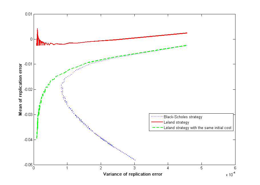
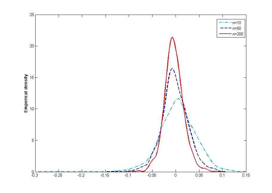
Figure 1: Mean-variance of Leland strategy and its normalized corrected hedging error

The simulation results for the profit/loss V1nh(S1)subscriptsuperscript𝑉𝑛1subscript𝑆1V^{n}_{1}-h(S_{1}) in Figure 1(a) suggest that in the presence of transaction costs, Leland strategy outperforms 222 A strategy is better than the others if it offers the lowest risk for a given level of returns. In the literature, the expectation replication error, also known as the expectation profit and loss, seems to be a good return measure while the variance of replication error is the most popular risk measure. A highly-tolerant hedger would prefer a position with high mean replication error and a high risk, whereas a highly risk-averse hedger would prefer a point with a low risk and low mean replication. the Black-Scholes discrete delta strategy even when they starts with the same initial cost. The empirical distribution and density of the normalized corrected hedging error in the Pergamenschikov’s theorem [37] (see eq.(1.2)) are shown in Figure 1(b). It turns out that the corrected hedging empirically converges to a centered variable that likely behaves as a normal distribution but with an asymmetric tail.

As seen above, the Leland method is important for practical purposes since it requires only a small change in parameter of the well-known Black-Scholes framework which is widely used in practice. However, when volatility is random, say σ=σ(yt)𝜎𝜎subscript𝑦𝑡\sigma=\sigma(y_{t}) where ytsubscript𝑦𝑡y_{t} is another random process, the strategy is no longer available from the Cauchy problem (2.2). In fact, pricing and hedging in such stochastic volatility (SV) contexts are intrinsically different from the Leland model and even in the absence of trading costs, the option price strongly depends on volatility level and future information of the volatility process y𝑦y. To see this issue, let us assume that y𝑦y is a Markov process. By the iterative property of expectation, the option price exclusive of trading costs is then given by

C(t,x,y)=𝐄[CBS(t,x;K,σ¯)|yt=y],𝐶𝑡𝑥𝑦𝐄delimited-[]conditionalsubscript𝐶𝐵𝑆𝑡𝑥𝐾¯𝜎subscript𝑦𝑡𝑦C(t,x,y)={\bf E}[C_{\mathchoice{BS}{BS}{\lower 0.75346pt\hbox{$\scriptstyle BS$}}{\lower 0.75346pt\hbox{$\scriptscriptstyle BS$}}}(t,x;K,\overline{\sigma})|y_{t}=y], (2.3)

where K𝐾K is the strike price, CBSsubscript𝐶𝐵𝑆C_{\mathchoice{BS}{BS}{\lower 0.75346pt\hbox{$\scriptstyle BS$}}{\lower 0.75346pt\hbox{$\scriptscriptstyle BS$}}} is the Black-Scholes option price functional and σ¯¯𝜎\overline{\sigma} is the averaged volatility defined by

σ¯2=11tt1σ2(ys)ds.superscript¯𝜎211𝑡superscriptsubscript𝑡1superscript𝜎2subscript𝑦𝑠differential-d𝑠\overline{\sigma}^{2}=\frac{1}{1-t}\int_{t}^{1}\sigma^{2}(y_{s})\mathrm{d}s.

It means that the option price is the average of Black-Scholes price on all possible future trajectories of the volatility process y𝑦y, which in reality cannot be observed directly. Thus, the option price and hence hedging strategy in SV models are very complicated and usually studied via asymptotic analysis.

Now let us now turn our attention to the presence of transaction costs. The above discussion has emphasized that the well-known form (1.1) for adjusted volatility in Leland’s algorithm is no longer helpful from a practical point of view. Furthermore, even for local volatility models in which σ𝜎\sigma only depends on time and the spot price S𝑆S, it is technically difficult to show the existence of a solution to (2.2) since the differential operator is not uniformly parabolic. In addition, estimates for derivatives of the option price, which are essential for approximation analysis, are not easy to achieve, see e.g. [27].

Fortunately, a deep study on the approximation of the hedging error shows that the limit of the replication error does not strongly depend on the form of adjusted volatility but only on the last term κnnsubscript𝜅𝑛𝑛\kappa_{n}\sqrt{n} whenever the latter product diverges to infinity. This important observation means that a simpler form ϱκnnitalic-ϱsubscript𝜅𝑛𝑛\varrho\kappa_{n}\sqrt{n} with some constant ϱitalic-ϱ\varrho, can be used to obtain the same asymptotic property for the hedging error. This modification is fully investigated for SV models in [33, 32]. Note that the option price and hedging strategy can be easily obtained if the new form is applied for the Cauchy problem (2.2) while it is impossible in practice for the classical one (1.1). In this paper we show that this suggestion is still useful even when jumps in the asset price and/or in stochastic volatility are taken into account.

We conclude the section by mentioning some important features of hedging in jumps models. First, jump risks cannot be covered by simply using the classical delta strategy even with a continuous-time adjustment policy. Second, if jumps are allowed in the stock price then one should distinguish two types of hedging errors: one is due to the market incompleteness concerning jumps and the other one is due to the discrete nature of the hedging portfolio. These two types of hedging errors have different behaviors. The literature of discrete hedging with jumps is vast and we only mention to [40, 39] for recent achievements. However, none of these mentioned papers discuss about trading costs.

3 Model with jumps and main results

3.1 The market model

Let (Ω,1,(t)0t1,𝐏)Ωsubscript1subscriptsubscript𝑡0𝑡1𝐏\left(\Omega,\mathcal{F}_{1},\left(\mathcal{F}_{\mathchoice{t}{t}{\lower 0.75346pt\hbox{$\scriptstyle t$}}{\lower 0.75346pt\hbox{$\scriptscriptstyle t$}}}\right)_{0\leq t\leq 1},\mathbf{P}\right) be the standard filtered probability space with two standard independent (t)0t1subscriptsubscript𝑡0𝑡1\left(\mathcal{F}_{\mathchoice{t}{t}{\lower 0.75346pt\hbox{$\scriptstyle t$}}{\lower 0.75346pt\hbox{$\scriptscriptstyle t$}}}\right)_{0\leq t\leq 1} adapted Wiener processes (Wt(1))superscriptsubscript𝑊𝑡1(W_{\mathchoice{t}{t}{\lower 0.75346pt\hbox{$\scriptstyle t$}}{\lower 0.75346pt\hbox{$\scriptscriptstyle t$}}}^{\left(1\right)}) and (Wt(2))superscriptsubscript𝑊𝑡2(W_{\mathchoice{t}{t}{\lower 0.75346pt\hbox{$\scriptstyle t$}}{\lower 0.75346pt\hbox{$\scriptscriptstyle t$}}}^{\left(2\right)}) taking values in \mathbb{R}. Consider a financial market that consists of one non-risky asset set as the numéraire and the risky one (e.g. stock) Stsubscript𝑆𝑡S_{\mathchoice{t}{t}{\lower 0.75346pt\hbox{$\scriptstyle t$}}{\lower 0.75346pt\hbox{$\scriptscriptstyle t$}}} defined as

{dSt=St(btdt+σ(yt)dWt(1)+dζt),dyt=α1(t,yt)dt+α2(t,yt)dWt(2),casesdsubscript𝑆𝑡subscript𝑆superscript𝑡subscript𝑏𝑡d𝑡𝜎subscript𝑦𝑡dsuperscriptsubscript𝑊𝑡1dsubscript𝜁𝑡dsubscript𝑦𝑡subscript𝛼1𝑡subscript𝑦𝑡d𝑡subscript𝛼2𝑡subscript𝑦𝑡dsubscriptsuperscript𝑊2𝑡\left\{\begin{array}[]{l}\mathrm{d}S_{\mathchoice{t}{t}{\lower 0.75346pt\hbox{$\scriptstyle t$}}{\lower 0.75346pt\hbox{$\scriptscriptstyle t$}}}=S_{\mathchoice{t^{-}}{t^{-}}{\lower 0.75346pt\hbox{$\scriptstyle t^{-}$}}{\lower 0.75346pt\hbox{$\scriptscriptstyle t^{-}$}}}\left(b_{t}\mathrm{d}t+\sigma\left(y_{\mathchoice{t}{t}{\lower 0.75346pt\hbox{$\scriptstyle t$}}{\lower 0.75346pt\hbox{$\scriptscriptstyle t$}}}\right)\mathrm{d}W_{\mathchoice{t}{t}{\lower 0.75346pt\hbox{$\scriptstyle t$}}{\lower 0.75346pt\hbox{$\scriptscriptstyle t$}}}^{\left(1\right)}+\mathrm{d}\zeta_{\mathchoice{t}{t}{\lower 0.75346pt\hbox{$\scriptstyle t$}}{\lower 0.75346pt\hbox{$\scriptscriptstyle t$}}}\right),\\ \mathrm{d}y_{\mathchoice{t}{t}{\lower 0.75346pt\hbox{$\scriptstyle t$}}{\lower 0.75346pt\hbox{$\scriptscriptstyle t$}}}=\alpha_{1}\left(t,y_{\mathchoice{t}{t}{\lower 0.75346pt\hbox{$\scriptstyle t$}}{\lower 0.75346pt\hbox{$\scriptscriptstyle t$}}}\right)\mathrm{d}t+\alpha_{2}\left(t,y_{\mathchoice{t}{t}{\lower 0.75346pt\hbox{$\scriptstyle t$}}{\lower 0.75346pt\hbox{$\scriptscriptstyle t$}}}\right)\mathrm{d}W^{(2)}_{\mathchoice{t}{t}{\lower 0.75346pt\hbox{$\scriptstyle t$}}{\lower 0.75346pt\hbox{$\scriptscriptstyle t$}}},\end{array}\right. (3.1)

where St=limstSssubscript𝑆superscript𝑡subscript𝑠𝑡subscript𝑆𝑠S_{\mathchoice{t^{-}}{t^{-}}{\lower 0.75346pt\hbox{$\scriptstyle t^{-}$}}{\lower 0.75346pt\hbox{$\scriptscriptstyle t^{-}$}}}=\lim_{s\uparrow t}S_{s} and the jump Lévy process is defined as

ζt=x(Jν)t,subscript𝜁𝑡𝑥subscript𝐽𝜈𝑡\zeta_{\mathchoice{t}{t}{\lower 0.75346pt\hbox{$\scriptstyle t$}}{\lower 0.75346pt\hbox{$\scriptscriptstyle t$}}}=x*(J-\nu)_{\mathchoice{t}{t}{\lower 0.75346pt\hbox{$\scriptstyle t$}}{\lower 0.75346pt\hbox{$\scriptscriptstyle t$}}}, (3.2)

which is independent of the Wiener processes (Wt(1))superscriptsubscript𝑊𝑡1(W_{\mathchoice{t}{t}{\lower 0.75346pt\hbox{$\scriptstyle t$}}{\lower 0.75346pt\hbox{$\scriptscriptstyle t$}}}^{\left(1\right)}) and (Wt(2))superscriptsubscript𝑊𝑡2(W_{\mathchoice{t}{t}{\lower 0.75346pt\hbox{$\scriptstyle t$}}{\lower 0.75346pt\hbox{$\scriptscriptstyle t$}}}^{\left(2\right)}). Here J(dt,dx)𝐽d𝑡d𝑥J(\mathrm{d}t,\mathrm{d}x) is the jump random measure of ζ𝜁\zeta having the deterministic compensator ν(dt,dx)=dtΠ(dx)𝜈d𝑡d𝑥d𝑡Πd𝑥\nu(\mathrm{d}t,\mathrm{d}x)=\mathrm{d}t\,\Pi(\mathrm{d}x), where Π()Π\Pi(\cdot) is the Lévy measure defined for any Borel set A={0}𝐴subscript0A\subseteq{\mathbb{R}}_{\mathchoice{*}{*}{\lower 0.75346pt\hbox{$\scriptstyle*$}}{\lower 0.75346pt\hbox{$\scriptscriptstyle*$}}}={\mathbb{R}}\setminus\{0\} as

Π(A)=𝐄0s1𝟏{ΔζsA}andΔζs=ζsζs.formulae-sequenceΠ𝐴𝐄subscript0𝑠1subscript1Δsubscript𝜁𝑠𝐴andΔsubscript𝜁𝑠subscript𝜁𝑠subscript𝜁limit-from𝑠\Pi(A)={\bf E}\,\sum_{\mathchoice{0\leq s\leq 1}{0\leq s\leq 1}{\lower 0.75346pt\hbox{$\scriptstyle 0\leq s\leq 1$}}{\lower 0.75346pt\hbox{$\scriptscriptstyle 0\leq s\leq 1$}}}{\bf 1}_{\mathchoice{\{\Delta\zeta_{\mathchoice{s}{s}{\lower 0.5382pt\hbox{$\scriptstyle s$}}{\lower 0.5382pt\hbox{$\scriptscriptstyle s$}}}\in A\}}{\{\Delta\zeta_{\mathchoice{s}{s}{\lower 0.5382pt\hbox{$\scriptstyle s$}}{\lower 0.5382pt\hbox{$\scriptscriptstyle s$}}}\in A\}}{\lower 0.75346pt\hbox{$\scriptstyle\{\Delta\zeta_{\mathchoice{s}{s}{\lower 0.37672pt\hbox{$\scriptstyle s$}}{\lower 0.37672pt\hbox{$\scriptscriptstyle s$}}}\in A\}$}}{\lower 0.75346pt\hbox{$\scriptscriptstyle\{\Delta\zeta_{\mathchoice{s}{s}{\lower 0.37672pt\hbox{$\scriptstyle s$}}{\lower 0.37672pt\hbox{$\scriptscriptstyle s$}}}\in A\}$}}}\quad\mbox{and}\quad\Delta\zeta_{\mathchoice{s}{s}{\lower 0.75346pt\hbox{$\scriptstyle s$}}{\lower 0.75346pt\hbox{$\scriptscriptstyle s$}}}=\zeta_{\mathchoice{s}{s}{\lower 0.75346pt\hbox{$\scriptstyle s$}}{\lower 0.75346pt\hbox{$\scriptscriptstyle s$}}}-\zeta_{\mathchoice{s-}{s-}{\lower 0.75346pt\hbox{$\scriptstyle s-$}}{\lower 0.75346pt\hbox{$\scriptscriptstyle s-$}}}. (3.3)

In order for Stsubscript𝑆𝑡S_{\mathchoice{t}{t}{\lower 0.75346pt\hbox{$\scriptstyle t$}}{\lower 0.75346pt\hbox{$\scriptscriptstyle t$}}} to be positive we assume that Π(],1])=0\Pi(]-\infty,-1])=0. Moreover, we assume that

Π(x2)=z2Π(dz)<.Πsuperscript𝑥2subscriptsubscriptsuperscript𝑧2Πd𝑧\Pi(x^{2})=\int_{\mathchoice{{\mathbb{R}}_{*}}{{\mathbb{R}}_{*}}{\lower 0.75346pt\hbox{$\scriptstyle{\mathbb{R}}_{*}$}}{\lower 0.75346pt\hbox{$\scriptscriptstyle{\mathbb{R}}_{*}$}}}z^{2}\Pi(\mathrm{d}z)<\infty. (3.4)

In the sequel we use the notation Π(f)=f(z)Π(dz)Π𝑓subscriptsubscript𝑓𝑧Πd𝑧\Pi(f)=\int_{\mathchoice{{\mathbb{R}}_{*}}{{\mathbb{R}}_{*}}{\lower 0.75346pt\hbox{$\scriptstyle{\mathbb{R}}_{*}$}}{\lower 0.75346pt\hbox{$\scriptscriptstyle{\mathbb{R}}_{*}$}}}f(z)\Pi(\mathrm{d}z). We recall that the symbol * means the stochastic integral, i.e. for any t>0𝑡0t>0 and any function h:[0,t]×:0𝑡h:[0,t]\times{\mathbb{R}}\to{\mathbb{R}},

h(Jν)t=0th(u,x)dJ~(du,dx),J~(dt,dx)=(Jν)(dt,dx).formulae-sequencesubscript𝐽𝜈𝑡subscriptsuperscript𝑡0subscriptsubscript𝑢𝑥differential-d~𝐽d𝑢d𝑥~𝐽d𝑡d𝑥𝐽𝜈d𝑡d𝑥h*(J-\nu)_{\mathchoice{t}{t}{\lower 0.75346pt\hbox{$\scriptstyle t$}}{\lower 0.75346pt\hbox{$\scriptscriptstyle t$}}}=\int^{t}_{\mathchoice{0}{0}{\lower 0.75346pt\hbox{$\scriptstyle 0$}}{\lower 0.75346pt\hbox{$\scriptscriptstyle 0$}}}\,\int_{{\mathbb{R}}_{\mathchoice{*}{*}{\lower 0.5382pt\hbox{$\scriptstyle*$}}{\lower 0.5382pt\hbox{$\scriptscriptstyle*$}}}}\,h(u,x)\,\mathrm{d}\widetilde{J}(\mathrm{d}u\,,\,\mathrm{d}x)\,,\quad\widetilde{J}(\mathrm{d}t\,,\,\mathrm{d}x)=(J-\nu)(\mathrm{d}t\,,\mathrm{d}x).

We assume that the coefficients αi,i=1,2formulae-sequencesubscript𝛼𝑖𝑖12\alpha_{i},i=1,2 are locally Lipschitz and linearly growth functions, which provides the existence of the unique strong solution y𝑦y to the second equation [16]. Moreover, we assume that the processes (Wt(1))0t1subscriptsubscriptsuperscript𝑊1𝑡0𝑡1(W^{(1)}_{\mathchoice{t}{t}{\lower 0.75346pt\hbox{$\scriptstyle t$}}{\lower 0.75346pt\hbox{$\scriptscriptstyle t$}}})_{\mathchoice{0\leq t\leq 1}{0\leq t\leq 1}{\lower 0.75346pt\hbox{$\scriptstyle 0\leq t\leq 1$}}{\lower 0.75346pt\hbox{$\scriptscriptstyle 0\leq t\leq 1$}}}, (Wt(2))0t1subscriptsubscriptsuperscript𝑊2𝑡0𝑡1(W^{(2)}_{\mathchoice{t}{t}{\lower 0.75346pt\hbox{$\scriptstyle t$}}{\lower 0.75346pt\hbox{$\scriptscriptstyle t$}}})_{\mathchoice{0\leq t\leq 1}{0\leq t\leq 1}{\lower 0.75346pt\hbox{$\scriptstyle 0\leq t\leq 1$}}{\lower 0.75346pt\hbox{$\scriptscriptstyle 0\leq t\leq 1$}}} and (ζt)0t1subscriptsubscript𝜁𝑡0𝑡1(\zeta_{\mathchoice{t}{t}{\lower 0.75346pt\hbox{$\scriptstyle t$}}{\lower 0.75346pt\hbox{$\scriptscriptstyle t$}}})_{\mathchoice{0\leq t\leq 1}{0\leq t\leq 1}{\lower 0.75346pt\hbox{$\scriptstyle 0\leq t\leq 1$}}{\lower 0.75346pt\hbox{$\scriptscriptstyle 0\leq t\leq 1$}}} are independent. Note that, if the volatility function σ()𝜎\sigma(\cdot) is constant, we obtain a Lévy financial market, which is very popular in the finance, see e.g. [21] and the references therein. We assume further that Δζt>1Δsubscript𝜁𝑡1\Delta\zeta_{\mathchoice{t}{t}{\lower 0.75346pt\hbox{$\scriptstyle t$}}{\lower 0.75346pt\hbox{$\scriptscriptstyle t$}}}>-1, i.e. Π(,1])=0\Pi(-\infty\,,\,-1])=0. So, in this case using the Doléans-Dade exponent we can represent the price process as

St=S0exp{0tbˇudu+0tσ(ys)dWs(1)+ζˇt},subscript𝑆𝑡subscript𝑆0superscriptsubscript0𝑡subscriptˇ𝑏𝑢differential-d𝑢superscriptsubscript0𝑡𝜎subscript𝑦𝑠differential-dsubscriptsuperscript𝑊1𝑠subscriptˇ𝜁𝑡S_{\mathchoice{t}{t}{\lower 0.75346pt\hbox{$\scriptstyle t$}}{\lower 0.75346pt\hbox{$\scriptscriptstyle t$}}}=S_{\mathchoice{0}{0}{\lower 0.75346pt\hbox{$\scriptstyle 0$}}{\lower 0.75346pt\hbox{$\scriptscriptstyle 0$}}}\exp\left\{\int_{0}^{t}\check{b}_{\mathchoice{u}{u}{\lower 0.75346pt\hbox{$\scriptstyle u$}}{\lower 0.75346pt\hbox{$\scriptscriptstyle u$}}}\,\mathrm{d}u+\int_{0}^{t}\sigma\left(y_{s}\right)\mathrm{d}W^{(1)}_{s}+\check{\zeta}_{\mathchoice{t}{t}{\lower 0.75346pt\hbox{$\scriptstyle t$}}{\lower 0.75346pt\hbox{$\scriptscriptstyle t$}}}\right\}, (3.5)

where ζˇt=ln(1+x)(Jν)tsubscriptˇ𝜁𝑡1𝑥subscript𝐽𝜈𝑡\check{\zeta}_{\mathchoice{t}{t}{\lower 0.75346pt\hbox{$\scriptstyle t$}}{\lower 0.75346pt\hbox{$\scriptscriptstyle t$}}}=\ln(1+x)*(J-\nu)_{\mathchoice{t}{t}{\lower 0.75346pt\hbox{$\scriptstyle t$}}{\lower 0.75346pt\hbox{$\scriptscriptstyle t$}}} and bˇt=btσ2(yt)/2+Π(ln(1+x)x)subscriptˇ𝑏𝑡subscript𝑏𝑡superscript𝜎2subscript𝑦𝑡2Π1𝑥𝑥\check{b}_{\mathchoice{t}{t}{\lower 0.75346pt\hbox{$\scriptstyle t$}}{\lower 0.75346pt\hbox{$\scriptscriptstyle t$}}}=b_{\mathchoice{t}{t}{\lower 0.75346pt\hbox{$\scriptstyle t$}}{\lower 0.75346pt\hbox{$\scriptscriptstyle t$}}}-\sigma^{2}(y_{\mathchoice{t}{t}{\lower 0.75346pt\hbox{$\scriptstyle t$}}{\lower 0.75346pt\hbox{$\scriptscriptstyle t$}}})/2+\Pi(\ln(1+x)-x).

Note that the Lévy measure defined in (3.3) may be infinite, i.e. Π()=+Πsubscript\Pi({\mathbb{R}}_{\mathchoice{*}{*}{\lower 0.75346pt\hbox{$\scriptstyle*$}}{\lower 0.75346pt\hbox{$\scriptscriptstyle*$}}})=+\infty. If θ=Π()<𝜃Πsubscript\theta=\Pi({\mathbb{R}}_{\mathchoice{*}{*}{\lower 0.75346pt\hbox{$\scriptstyle*$}}{\lower 0.75346pt\hbox{$\scriptscriptstyle*$}}})<\infty, we can represent the jump process in (3.1) as

ζt=j=1Ntξjθ𝐄ξ1t,subscript𝜁𝑡superscriptsubscript𝑗1subscript𝑁𝑡subscript𝜉𝑗𝜃𝐄subscript𝜉1𝑡\zeta_{\mathchoice{t}{t}{\lower 0.75346pt\hbox{$\scriptstyle t$}}{\lower 0.75346pt\hbox{$\scriptscriptstyle t$}}}=\sum_{j=1}^{N_{\mathchoice{t}{t}{\lower 0.5382pt\hbox{$\scriptstyle t$}}{\lower 0.5382pt\hbox{$\scriptscriptstyle t$}}}}\xi_{j}-\theta{\bf E}\xi_{\mathchoice{1}{1}{\lower 0.75346pt\hbox{$\scriptstyle 1$}}{\lower 0.75346pt\hbox{$\scriptscriptstyle 1$}}}\,t, (3.6)

where (Nt)t0subscriptsubscript𝑁𝑡𝑡0(N_{\mathchoice{t}{t}{\lower 0.75346pt\hbox{$\scriptstyle t$}}{\lower 0.75346pt\hbox{$\scriptscriptstyle t$}}})_{\mathchoice{t\geq 0}{t\geq 0}{\lower 0.75346pt\hbox{$\scriptstyle t\geq 0$}}{\lower 0.75346pt\hbox{$\scriptscriptstyle t\geq 0$}}} is a Poisson process with intensity parameter θ𝜃\theta and (ξj)j1subscriptsubscript𝜉𝑗𝑗1(\xi_{j})_{\mathchoice{j\geq 1}{j\geq 1}{\lower 0.75346pt\hbox{$\scriptstyle j\geq 1$}}{\lower 0.75346pt\hbox{$\scriptscriptstyle j\geq 1$}}} are i.i.d. random variables taking values in (1,+)1(-1,+\infty). We assume further that the Poisson process Ntsubscript𝑁𝑡N_{t} and the jumps sizes (ξj)j1subscriptsubscript𝜉𝑗𝑗1(\xi_{j})_{\mathchoice{j\geq 1}{j\geq 1}{\lower 0.75346pt\hbox{$\scriptstyle j\geq 1$}}{\lower 0.75346pt\hbox{$\scriptscriptstyle j\geq 1$}}} are independent. In this case, the stock price can be expressed as

St=S0exp{0tbˇudu+0tσ(ys)dWs(1)+j=1Ntln(1+ξj)},subscript𝑆𝑡subscript𝑆0superscriptsubscript0𝑡subscriptˇ𝑏𝑢differential-d𝑢superscriptsubscript0𝑡𝜎subscript𝑦𝑠differential-dsubscriptsuperscript𝑊1𝑠superscriptsubscript𝑗1subscript𝑁𝑡1subscript𝜉𝑗S_{\mathchoice{t}{t}{\lower 0.75346pt\hbox{$\scriptstyle t$}}{\lower 0.75346pt\hbox{$\scriptscriptstyle t$}}}=S_{0}\exp\left\{\int_{0}^{t}\check{b}_{\mathchoice{u}{u}{\lower 0.75346pt\hbox{$\scriptstyle u$}}{\lower 0.75346pt\hbox{$\scriptscriptstyle u$}}}\,\mathrm{d}u+\int_{0}^{t}\sigma\left(y_{s}\right)\mathrm{d}W^{(1)}_{s}+\sum_{j=1}^{N_{\mathchoice{t}{t}{\lower 0.5382pt\hbox{$\scriptstyle t$}}{\lower 0.5382pt\hbox{$\scriptscriptstyle t$}}}}\ln\left(1+\xi_{j}\right)\right\}, (3.7)

where bˇt=btσ2(yt)/2θ𝐄ξ1subscriptˇ𝑏𝑡subscript𝑏𝑡superscript𝜎2subscript𝑦𝑡2𝜃𝐄subscript𝜉1\check{b}_{\mathchoice{t}{t}{\lower 0.75346pt\hbox{$\scriptstyle t$}}{\lower 0.75346pt\hbox{$\scriptscriptstyle t$}}}=b_{\mathchoice{t}{t}{\lower 0.75346pt\hbox{$\scriptstyle t$}}{\lower 0.75346pt\hbox{$\scriptscriptstyle t$}}}-\sigma^{2}(y_{\mathchoice{t}{t}{\lower 0.75346pt\hbox{$\scriptstyle t$}}{\lower 0.75346pt\hbox{$\scriptscriptstyle t$}}})/2-\theta{\bf E}\,\xi_{\mathchoice{1}{1}{\lower 0.75346pt\hbox{$\scriptstyle 1$}}{\lower 0.75346pt\hbox{$\scriptscriptstyle 1$}}}.

Remark 1.

The drift btsubscript𝑏𝑡b_{t} plays no role in approximation. In fact, our asymptotic results are valid for any btsubscript𝑏𝑡b_{t} satisfying sup0t1𝐄|bt|<subscriptsupremum0𝑡1𝐄subscript𝑏𝑡\sup_{0\leq t\leq 1}{\bf E}|b_{t}|<\infty.

Remark 2.

In this paper we will not discuss about the problem of change of measure and the jump risk but we accept the free-risk assumption of asset dynamics as the starting point. Clearly, a jump-diffusion setting leads to an incomplete market, which is also an important feature of stochastic volatility settings. Hence, there are many ways to choose the pricing measure via Girsanov’s technique. Such a procedure makes an essential change not only on the diffusion but also on the jump part of the asset dynamics [9, 31]. In [24], an expectation equilibrium argument is used to obtain a simple transform from the original physical probability to a risk-neutral probability for which many assets (bonds, stocks, derivatives on stocks) can be simultaneously priced in the same framework.

3.2 Assumptions and examples

The following condition on the jump sizes is accepted in our consideration:

(𝐂1)subscript𝐂1({\bf C}_{1}) The Lévy measure of jump sizes satisfies

Π()<and(1,0](1+z)1Π(dz)<.formulae-sequenceΠsubscriptandsubscript10superscript1𝑧1Πd𝑧\Pi({\mathbb{R}}_{\mathchoice{*}{*}{\lower 0.75346pt\hbox{$\scriptstyle*$}}{\lower 0.75346pt\hbox{$\scriptscriptstyle*$}}})<\infty\quad\mbox{and}\quad\int_{\mathchoice{(-1,0]}{(-1,0]}{\lower 0.75346pt\hbox{$\scriptstyle(-1,0]$}}{\lower 0.75346pt\hbox{$\scriptscriptstyle(-1,0]$}}}(1+z)^{-1}{\Pi(\mathrm{d}z)}<\infty.

The first integrability condition is nothing than the condition of finite variance for the jump size distribution. The second one is equivalent to 𝐄(1+ξ)1<𝐄superscript1𝜉1{\bf E}(1+\xi)^{-1}<\infty. These conditions are not too strong and automatically fulfilled in Merton jump-diffusion models [31] where the jump size distribution is assumed to be log-normal. In [24] within an equilibrium-based setting, log-exponential distributions are suggested to achieve convenient features in an analytical calculation. Note that this family of jump size distributions also satisfies Condition (𝐂1)subscript𝐂1({\bf C}_{1}).

Let us turn our attention to volatility assumptions. Following [33] we assume that the volatility process satisfies the integrable condition.

(𝐂2)subscript𝐂2({\bf C}_{2}) σ𝜎\sigma is a twice continuously differentiable function satisfying

0<σmininfyσ(y)andsup0t1𝐄max{σ(yt),|σ(yt)|}<.formulae-sequence0subscript𝜎subscriptinfimum𝑦𝜎𝑦andsubscriptsupremum0𝑡1𝐄𝜎subscript𝑦𝑡superscript𝜎subscript𝑦𝑡0<\sigma_{\mathchoice{\min}{\min}{\lower 0.75346pt\hbox{$\scriptstyle\min$}}{\lower 0.75346pt\hbox{$\scriptscriptstyle\min$}}}\leq\inf_{\mathchoice{y\in{\mathbb{R}}}{y\in{\mathbb{R}}}{\lower 0.75346pt\hbox{$\scriptstyle y\in{\mathbb{R}}$}}{\lower 0.75346pt\hbox{$\scriptscriptstyle y\in{\mathbb{R}}$}}}\sigma(y)\quad\mbox{and}\quad\sup_{\mathchoice{0\leq t\leq 1}{0\leq t\leq 1}{\lower 0.75346pt\hbox{$\scriptstyle 0\leq t\leq 1$}}{\lower 0.75346pt\hbox{$\scriptscriptstyle 0\leq t\leq 1$}}}{\bf E}\,\max\{\sigma(y_{t}),|\sigma^{\prime}(y_{t})|\}<\infty.

In fact, Condition (𝐂2)subscript𝐂2({\bf C}_{2}) is fulfilled for almost widely used stochastic volatility models, see [33] for more discussions.

Remark 3.

Remark that in the present setting, the combination of stochastic volatility and jumps means that the asset price is not a Lévy process but a semi-martingale. As mentioned in [33], finite moments of the asset process in SV models are not guaranteed in general, see [2, 29]. This crucial feature prevent us from making an L2superscript𝐿2L^{2}-based approximation as in deterministic volatility models [22, 27, 28]. Therefore, for the approximation procedures below we follow the approach in [33, 34] which is based on a truncation technique. The convergence results obtained in what follows are only achieved in probability.

We conclude this subsection with some well-known stochastic volatility models with jumps, see [9] and Section 4 for more examples.

Bates model: The Bates model is a jump-diffusion stochastic volatility model obtained by adding proportional log-normal jumps to the Heston stochastic volatility model:

dSt=St(a0dt+ytdWtS+dZt);dyt=a(myt)dt+bytdWty,formulae-sequencedsubscript𝑆𝑡subscript𝑆𝑡subscript𝑎0d𝑡subscript𝑦𝑡dsuperscriptsubscript𝑊𝑡𝑆dsubscript𝑍𝑡dsubscript𝑦𝑡𝑎𝑚subscript𝑦𝑡d𝑡𝑏subscript𝑦𝑡dsuperscriptsubscript𝑊𝑡𝑦\mathrm{d}S_{t}=S_{t}(a_{\mathchoice{0}{0}{\lower 0.75346pt\hbox{$\scriptstyle 0$}}{\lower 0.75346pt\hbox{$\scriptscriptstyle 0$}}}\mathrm{d}t+\sqrt{y_{t}}\mathrm{d}W_{t}^{S}+\mathrm{d}Z_{t});\quad\mathrm{d}y_{t}=a(m-y_{t})\mathrm{d}t+b\sqrt{y_{t}}\mathrm{d}W_{t}^{y}, (3.8)

where WS,Wysuperscript𝑊𝑆superscript𝑊𝑦W^{S},W^{y} are Brownian motions with correlation ρ𝜌\rho and Z𝑍Z is a compound Poisson process with intensity θ𝜃\theta and log-normal distribution. Condition (𝐂1)subscript𝐂1({\bf C}_{1}) is clearly verified since jumps follow the log-normal law. The Bates model exhibits some nice properties from a practical point of view. Firstly, the characteristic function of the log-price is available in a closed-form, which is important for pricing purposes. Secondly, the implied volatility pattern for long term and short term options can be adjusted separately [9].

Ornstein-Uhlenbeck stochastic volatility models: It is possible to introduce a jump component in both price and volatility processes. Such models are suggested by Barndorff-Nielsen and Shephard to take leverage effects into account:

St=S0eXt,dXt=(a0+a1σt2)dt+σtdWt+ρdZt,dσt2=θσt2dt+dZt.formulae-sequencesubscript𝑆𝑡subscript𝑆0superscript𝑒subscript𝑋𝑡formulae-sequencedsubscript𝑋𝑡subscript𝑎0subscript𝑎1superscriptsubscript𝜎𝑡2d𝑡subscript𝜎𝑡dsubscript𝑊𝑡𝜌dsubscript𝑍𝑡dsuperscriptsubscript𝜎𝑡2𝜃superscriptsubscript𝜎𝑡2d𝑡dsubscript𝑍𝑡S_{\mathchoice{t}{t}{\lower 0.75346pt\hbox{$\scriptstyle t$}}{\lower 0.75346pt\hbox{$\scriptscriptstyle t$}}}=S_{\mathchoice{0}{0}{\lower 0.75346pt\hbox{$\scriptstyle 0$}}{\lower 0.75346pt\hbox{$\scriptscriptstyle 0$}}}\,e^{X_{\mathchoice{t}{t}{\lower 0.5382pt\hbox{$\scriptstyle t$}}{\lower 0.5382pt\hbox{$\scriptscriptstyle t$}}}}\,,\quad\mathrm{d}X_{\mathchoice{t}{t}{\lower 0.75346pt\hbox{$\scriptstyle t$}}{\lower 0.75346pt\hbox{$\scriptscriptstyle t$}}}=(a_{\mathchoice{0}{0}{\lower 0.75346pt\hbox{$\scriptstyle 0$}}{\lower 0.75346pt\hbox{$\scriptscriptstyle 0$}}}+a_{\mathchoice{1}{1}{\lower 0.75346pt\hbox{$\scriptstyle 1$}}{\lower 0.75346pt\hbox{$\scriptscriptstyle 1$}}}\sigma_{t}^{2})\mathrm{d}t+\sigma_{t}\mathrm{d}W_{t}+\rho\mathrm{d}Z_{\mathchoice{t}{t}{\lower 0.75346pt\hbox{$\scriptstyle t$}}{\lower 0.75346pt\hbox{$\scriptscriptstyle t$}}}\,,\quad\mathrm{d}\sigma_{t}^{2}=-\theta\sigma_{t}^{2}\mathrm{d}t+\mathrm{d}Z_{t}. (3.9)

If ρ=0𝜌0\rho=0 the volatility moves with jumps but the price process has continuous paths. The case ρ0𝜌0\rho\neq 0, representing a strong correlation between volatility and price, is more flexible but computation is now challenging. Remark that in this case σ𝜎\sigma is not the ”true” volatility as the returns are also affected by changes of the Lévy process Ztsubscript𝑍𝑡Z_{t}. If jumps still follow a log-normal law then Condition (𝐂1)subscript𝐂1({\bf C}_{1}) is fulfilled.

3.3 Approximate hedging with transaction costs: main result

In this section, we study the problem of discrete hedging under proportional transaction costs using the increasing volatility principle as in Leland’s algorithm following the setting in [33]. More precisely, we suppose that for each successful transaction, traders are charged by a cost that is proportional to the trading volume with the cost coefficient κ𝜅\kappa. Here κ𝜅\kappa is a positive constant defined by market moderators. Let us suppose that the investor plans to revise his portfolio at dates (ti)subscript𝑡𝑖(t_{i}) defined by

ti=g(i/n),g(t)=1(1t)μ,1μ<2,formulae-sequencesubscript𝑡𝑖𝑔𝑖𝑛formulae-sequence𝑔𝑡1superscript1𝑡𝜇1𝜇2t_{i}=g\left(i/n\right),\quad g(t)=1-\left(1-t\right)^{\mu}\,,\quad 1\leq\mu<2\,, (3.10)

where n𝑛n is the number of revisions. The parameter μ𝜇\mu is used to control the rate of convergence of the replication error. The bigger value of μ𝜇\mu the more frequently the portfolio is revised. Clearly one gets the well-known uniform readjustment for μ=1𝜇1\mu=1.

To compensate transaction costs caused by hedging activities, the option seller is suggested to follow the Leland strategy defined by the piecewise process

γtn=i=1nC^x(ti1,Sti1)𝟏(ti1,ti](t),superscriptsubscript𝛾𝑡𝑛superscriptsubscript𝑖1𝑛subscript^𝐶𝑥subscript𝑡𝑖1subscript𝑆subscript𝑡𝑖1subscript1subscript𝑡𝑖1subscript𝑡𝑖𝑡\gamma_{\mathchoice{t}{t}{\lower 0.75346pt\hbox{$\scriptstyle t$}}{\lower 0.75346pt\hbox{$\scriptscriptstyle t$}}}^{n}=\sum_{i=1}^{n}\hat{C}_{x}\left(t_{i-1},S_{t_{i-1}}\right)\mathbf{1}_{(t_{i-1},t_{i}]}\left(t\right), (3.11)

where C^^𝐶\widehat{C} is the solution to the following adjusted-volatility Black-Scholes PDE

Ct(t,x)+12σ^t2x2Cxx(t,x)=0,0t<1,C(1,x)=h(x):=(xK)+.formulae-sequenceformulae-sequencesubscript𝐶𝑡𝑡𝑥12superscriptsubscript^𝜎𝑡2superscript𝑥2subscript𝐶𝑥𝑥𝑡𝑥00𝑡1𝐶1𝑥𝑥assignsubscript𝑥𝐾C_{\mathchoice{t}{t}{\lower 0.75346pt\hbox{$\scriptstyle t$}}{\lower 0.75346pt\hbox{$\scriptscriptstyle t$}}}(t,x)+\frac{1}{2}\widehat{\sigma}_{t}^{2}x^{2}C_{\mathchoice{xx}{xx}{\lower 0.75346pt\hbox{$\scriptstyle xx$}}{\lower 0.75346pt\hbox{$\scriptscriptstyle xx$}}}(t,x)=0,\quad 0\leq t<1,\quad C(1,x)=h(x):=(x-K)_{\mathchoice{+}{+}{\lower 0.75346pt\hbox{$\scriptstyle+$}}{\lower 0.75346pt\hbox{$\scriptscriptstyle+$}}}\,. (3.12)

Here the adjusted volatility σ^2superscript^𝜎2\widehat{\sigma}^{2} is given by

σ^2(t)=ϱnf(t)withf(t)=g1(t)=1(1t)1/μ.formulae-sequencesuperscript^𝜎2𝑡italic-ϱ𝑛superscript𝑓𝑡with𝑓𝑡superscript𝑔1𝑡1superscript1𝑡1𝜇\widehat{\sigma}^{2}(t)=\varrho\sqrt{nf^{\prime}(t)}\quad\mbox{with}\quad f(t)=g^{-1}(t)=1-(1-t)^{1/\mu}. (3.13)

The motivation of this simple form is discussed in Section 2, see more in [33]. We remark that when volatility is deterministic the classical modified volatility form (1.1) can be used. This special case will be treated in Section 5. Now, using strategy γtnsuperscriptsubscript𝛾𝑡𝑛\gamma_{t}^{n} requires a cumulative trading volume measured in dollar value which is given by

Γn=i=1nSti|γtinγti1n|.subscriptΓ𝑛subscriptsuperscript𝑛𝑖1subscript𝑆subscript𝑡𝑖superscriptsubscript𝛾subscript𝑡𝑖𝑛superscriptsubscript𝛾subscript𝑡𝑖1𝑛\Gamma_{n}=\sum^{n}_{\mathchoice{i=1}{i=1}{\lower 0.75346pt\hbox{$\scriptstyle i=1$}}{\lower 0.75346pt\hbox{$\scriptscriptstyle i=1$}}}\,S_{\mathchoice{t_{\mathchoice{i}{i}{\lower 0.5382pt\hbox{$\scriptstyle i$}}{\lower 0.5382pt\hbox{$\scriptscriptstyle i$}}}}{t_{\mathchoice{i}{i}{\lower 0.5382pt\hbox{$\scriptstyle i$}}{\lower 0.5382pt\hbox{$\scriptscriptstyle i$}}}}{\lower 0.75346pt\hbox{$\scriptstyle t_{\mathchoice{i}{i}{\lower 0.37672pt\hbox{$\scriptstyle i$}}{\lower 0.37672pt\hbox{$\scriptscriptstyle i$}}}$}}{\lower 0.75346pt\hbox{$\scriptscriptstyle t_{\mathchoice{i}{i}{\lower 0.37672pt\hbox{$\scriptstyle i$}}{\lower 0.37672pt\hbox{$\scriptscriptstyle i$}}}$}}}|\gamma_{\mathchoice{t_{\mathchoice{i}{i}{\lower 0.5382pt\hbox{$\scriptstyle i$}}{\lower 0.5382pt\hbox{$\scriptscriptstyle i$}}}}{t_{\mathchoice{i}{i}{\lower 0.5382pt\hbox{$\scriptstyle i$}}{\lower 0.5382pt\hbox{$\scriptscriptstyle i$}}}}{\lower 0.75346pt\hbox{$\scriptstyle t_{\mathchoice{i}{i}{\lower 0.37672pt\hbox{$\scriptstyle i$}}{\lower 0.37672pt\hbox{$\scriptscriptstyle i$}}}$}}{\lower 0.75346pt\hbox{$\scriptscriptstyle t_{\mathchoice{i}{i}{\lower 0.37672pt\hbox{$\scriptstyle i$}}{\lower 0.37672pt\hbox{$\scriptscriptstyle i$}}}$}}}^{n}-\gamma_{\mathchoice{t_{\mathchoice{i-1}{i-1}{\lower 0.5382pt\hbox{$\scriptstyle i-1$}}{\lower 0.5382pt\hbox{$\scriptscriptstyle i-1$}}}}{t_{\mathchoice{i-1}{i-1}{\lower 0.5382pt\hbox{$\scriptstyle i-1$}}{\lower 0.5382pt\hbox{$\scriptscriptstyle i-1$}}}}{\lower 0.75346pt\hbox{$\scriptstyle t_{\mathchoice{i-1}{i-1}{\lower 0.37672pt\hbox{$\scriptstyle i-1$}}{\lower 0.37672pt\hbox{$\scriptscriptstyle i-1$}}}$}}{\lower 0.75346pt\hbox{$\scriptscriptstyle t_{\mathchoice{i-1}{i-1}{\lower 0.37672pt\hbox{$\scriptstyle i-1$}}{\lower 0.37672pt\hbox{$\scriptscriptstyle i-1$}}}$}}}^{n}|\,.

By Itô’s lemma one represents the payoff as

h(S1)subscript𝑆1\displaystyle h(S_{1}) =C^(0,S0)+01C^x(t,St)dStabsent^𝐶0subscript𝑆0superscriptsubscript01subscript^𝐶𝑥𝑡subscript𝑆superscript𝑡differential-dsubscript𝑆𝑡\displaystyle=\widehat{C}(0,S_{0})+\int_{0}^{1}\widehat{C}_{\mathchoice{x}{x}{\lower 0.75346pt\hbox{$\scriptstyle x$}}{\lower 0.75346pt\hbox{$\scriptscriptstyle x$}}}(t,S_{\mathchoice{t^{-}}{t^{-}}{\lower 0.75346pt\hbox{$\scriptstyle t^{-}$}}{\lower 0.75346pt\hbox{$\scriptscriptstyle t^{-}$}}})\mathrm{d}S_{t}
+01(C^t(t,St)+12σ2(yt)St2C^xx(t,St))dt+0t1𝐁(t,St,ΔSt/St),superscriptsubscript01subscript^𝐶𝑡𝑡subscript𝑆𝑡12superscript𝜎2subscript𝑦𝑡subscriptsuperscript𝑆2𝑡subscript^𝐶𝑥𝑥𝑡subscript𝑆𝑡differential-d𝑡subscript0𝑡1𝐁𝑡subscript𝑆superscript𝑡Δsubscript𝑆𝑡subscript𝑆superscript𝑡\displaystyle+\int_{0}^{1}\left(\widehat{C}_{\mathchoice{t}{t}{\lower 0.75346pt\hbox{$\scriptstyle t$}}{\lower 0.75346pt\hbox{$\scriptscriptstyle t$}}}(t,S_{\mathchoice{t}{t}{\lower 0.75346pt\hbox{$\scriptstyle t$}}{\lower 0.75346pt\hbox{$\scriptscriptstyle t$}}})+\frac{1}{2}\sigma^{2}(y_{t})S^{2}_{\mathchoice{t}{t}{\lower 0.75346pt\hbox{$\scriptstyle t$}}{\lower 0.75346pt\hbox{$\scriptscriptstyle t$}}}\widehat{C}_{\mathchoice{xx}{xx}{\lower 0.75346pt\hbox{$\scriptstyle xx$}}{\lower 0.75346pt\hbox{$\scriptscriptstyle xx$}}}(t,S_{\mathchoice{t}{t}{\lower 0.75346pt\hbox{$\scriptstyle t$}}{\lower 0.75346pt\hbox{$\scriptscriptstyle t$}}})\right)\mathrm{d}t+\sum_{\mathchoice{0\leq t\leq 1}{0\leq t\leq 1}{\lower 0.75346pt\hbox{$\scriptstyle 0\leq t\leq 1$}}{\lower 0.75346pt\hbox{$\scriptscriptstyle 0\leq t\leq 1$}}}\,{\bf B}(t,S_{\mathchoice{t^{-}}{t^{-}}{\lower 0.75346pt\hbox{$\scriptstyle t^{-}$}}{\lower 0.75346pt\hbox{$\scriptscriptstyle t^{-}$}}},\Delta S_{\mathchoice{t}{t}{\lower 0.75346pt\hbox{$\scriptstyle t$}}{\lower 0.75346pt\hbox{$\scriptscriptstyle t$}}}/S_{\mathchoice{t^{-}}{t^{-}}{\lower 0.75346pt\hbox{$\scriptstyle t^{-}$}}{\lower 0.75346pt\hbox{$\scriptscriptstyle t^{-}$}}})\,,

where 𝐁(t,x,z)=C^(t,x(z+1))C^(t,x)zxC^x(t,x)𝐁𝑡𝑥𝑧^𝐶𝑡𝑥𝑧1^𝐶𝑡𝑥𝑧𝑥subscript^𝐶𝑥𝑡𝑥{\bf B}(t,x,z)=\hat{C}\left(t,x(z+1)\right)-\hat{C}\left(t,x\right)-zx\hat{C}_{\mathchoice{x}{x}{\lower 0.75346pt\hbox{$\scriptstyle x$}}{\lower 0.75346pt\hbox{$\scriptscriptstyle x$}}}\left(t,x\right) and ΔSt=StStΔsubscript𝑆𝑡subscript𝑆𝑡subscript𝑆superscript𝑡\Delta S_{\mathchoice{t}{t}{\lower 0.75346pt\hbox{$\scriptstyle t$}}{\lower 0.75346pt\hbox{$\scriptscriptstyle t$}}}=S_{\mathchoice{t}{t}{\lower 0.75346pt\hbox{$\scriptstyle t$}}{\lower 0.75346pt\hbox{$\scriptscriptstyle t$}}}-S_{\mathchoice{t^{-}}{t^{-}}{\lower 0.75346pt\hbox{$\scriptstyle t^{-}$}}{\lower 0.75346pt\hbox{$\scriptscriptstyle t^{-}$}}} is the jump size of the stock price at time t𝑡t. The above sum of jumps can be represented as

I3,n=01𝐁(t,St,z)J(dt,dz).subscript𝐼3𝑛superscriptsubscript01subscriptsubscript𝐁𝑡subscript𝑆superscript𝑡𝑧𝐽d𝑡d𝑧I_{\mathchoice{3,n}{3,n}{\lower 0.75346pt\hbox{$\scriptstyle 3,n$}}{\lower 0.75346pt\hbox{$\scriptscriptstyle 3,n$}}}=\int_{0}^{1}\int_{\mathchoice{{\mathbb{R}}_{\mathchoice{*}{*}{\lower 0.5382pt\hbox{$\scriptstyle*$}}{\lower 0.5382pt\hbox{$\scriptscriptstyle*$}}}}{{\mathbb{R}}_{\mathchoice{*}{*}{\lower 0.5382pt\hbox{$\scriptstyle*$}}{\lower 0.5382pt\hbox{$\scriptscriptstyle*$}}}}{\lower 0.75346pt\hbox{$\scriptstyle{\mathbb{R}}_{\mathchoice{*}{*}{\lower 0.37672pt\hbox{$\scriptstyle*$}}{\lower 0.37672pt\hbox{$\scriptscriptstyle*$}}}$}}{\lower 0.75346pt\hbox{$\scriptscriptstyle{\mathbb{R}}_{\mathchoice{*}{*}{\lower 0.37672pt\hbox{$\scriptstyle*$}}{\lower 0.37672pt\hbox{$\scriptscriptstyle*$}}}$}}}{\bf B}\left(t,S_{\mathchoice{t^{-}}{t^{-}}{\lower 0.75346pt\hbox{$\scriptstyle t^{-}$}}{\lower 0.75346pt\hbox{$\scriptscriptstyle t^{-}$}}},z\right){J}(\mathrm{d}t\,,\,\mathrm{d}z)\,. (3.14)

Assuming that the initial capital (option price) is given by V0n=C^(0,S0)subscriptsuperscript𝑉𝑛0^𝐶0subscript𝑆0V^{n}_{0}=\widehat{C}(0,S_{0}) and using (3.12), one represents 333Note that for Lebesgue and Itô’s integrals one can replace Stsubscript𝑆superscript𝑡S_{\mathchoice{t^{-}}{t^{-}}{\lower 0.75346pt\hbox{$\scriptstyle t^{-}$}}{\lower 0.75346pt\hbox{$\scriptscriptstyle t^{-}$}}} by Stsubscript𝑆𝑡S_{\mathchoice{t}{t}{\lower 0.75346pt\hbox{$\scriptstyle t$}}{\lower 0.75346pt\hbox{$\scriptscriptstyle t$}}}. the hedging error as

V1nh(S1)=12I1,n+I2,nI3,nκΓn,subscriptsuperscript𝑉𝑛1subscript𝑆112subscript𝐼1𝑛subscript𝐼2𝑛subscript𝐼3𝑛𝜅subscriptΓ𝑛\displaystyle V^{n}_{\mathchoice{1}{1}{\lower 0.75346pt\hbox{$\scriptstyle 1$}}{\lower 0.75346pt\hbox{$\scriptscriptstyle 1$}}}-h(S_{\mathchoice{1}{1}{\lower 0.75346pt\hbox{$\scriptstyle 1$}}{\lower 0.75346pt\hbox{$\scriptscriptstyle 1$}}})=\frac{1}{2}I_{\mathchoice{1,n}{1,n}{\lower 0.75346pt\hbox{$\scriptstyle 1,n$}}{\lower 0.75346pt\hbox{$\scriptscriptstyle 1,n$}}}+I_{\mathchoice{2,n}{2,n}{\lower 0.75346pt\hbox{$\scriptstyle 2,n$}}{\lower 0.75346pt\hbox{$\scriptscriptstyle 2,n$}}}-I_{\mathchoice{3,n}{3,n}{\lower 0.75346pt\hbox{$\scriptstyle 3,n$}}{\lower 0.75346pt\hbox{$\scriptscriptstyle 3,n$}}}-\kappa\Gamma_{n}, (3.15)

where I1,n=01(σ^t2σ2(yt))St2C^xx(t,St)dtsubscript𝐼1𝑛superscriptsubscript01superscriptsubscript^𝜎𝑡2superscript𝜎2subscript𝑦𝑡superscriptsubscript𝑆𝑡2subscript^𝐶𝑥𝑥𝑡subscript𝑆𝑡differential-d𝑡I_{\mathchoice{1,n}{1,n}{\lower 0.75346pt\hbox{$\scriptstyle 1,n$}}{\lower 0.75346pt\hbox{$\scriptscriptstyle 1,n$}}}=\int_{\mathchoice{0}{0}{\lower 0.75346pt\hbox{$\scriptstyle 0$}}{\lower 0.75346pt\hbox{$\scriptscriptstyle 0$}}}^{1}\,\left(\widehat{\sigma}_{\mathchoice{t}{t}{\lower 0.75346pt\hbox{$\scriptstyle t$}}{\lower 0.75346pt\hbox{$\scriptscriptstyle t$}}}^{2}-\sigma^{2}(y_{\mathchoice{t}{t}{\lower 0.75346pt\hbox{$\scriptstyle t$}}{\lower 0.75346pt\hbox{$\scriptscriptstyle t$}}})\right)\,S_{\mathchoice{t}{t}{\lower 0.75346pt\hbox{$\scriptstyle t$}}{\lower 0.75346pt\hbox{$\scriptscriptstyle t$}}}^{2}\widehat{C}_{\mathchoice{xx}{xx}{\lower 0.75346pt\hbox{$\scriptstyle xx$}}{\lower 0.75346pt\hbox{$\scriptscriptstyle xx$}}}(t,S_{\mathchoice{t}{t}{\lower 0.75346pt\hbox{$\scriptstyle t$}}{\lower 0.75346pt\hbox{$\scriptscriptstyle t$}}})\mathrm{d}t and I2,n=01(γtnC^x(t,St))dStsubscript𝐼2𝑛superscriptsubscript01superscriptsubscript𝛾superscript𝑡𝑛subscript^𝐶𝑥𝑡subscript𝑆superscript𝑡differential-dsubscript𝑆𝑡I_{\mathchoice{2,n}{2,n}{\lower 0.75346pt\hbox{$\scriptstyle 2,n$}}{\lower 0.75346pt\hbox{$\scriptscriptstyle 2,n$}}}=\int_{\mathchoice{0}{0}{\lower 0.75346pt\hbox{$\scriptstyle 0$}}{\lower 0.75346pt\hbox{$\scriptscriptstyle 0$}}}^{1}\left(\gamma_{\mathchoice{t^{-}}{t^{-}}{\lower 0.75346pt\hbox{$\scriptstyle t^{-}$}}{\lower 0.75346pt\hbox{$\scriptscriptstyle t^{-}$}}}^{n}-\widehat{C}_{\mathchoice{x}{x}{\lower 0.75346pt\hbox{$\scriptstyle x$}}{\lower 0.75346pt\hbox{$\scriptscriptstyle x$}}}(t,S_{\mathchoice{t^{-}}{t^{-}}{\lower 0.75346pt\hbox{$\scriptstyle t^{-}$}}{\lower 0.75346pt\hbox{$\scriptscriptstyle t^{-}$}}})\right)\mathrm{d}S_{\mathchoice{t}{t}{\lower 0.75346pt\hbox{$\scriptstyle t$}}{\lower 0.75346pt\hbox{$\scriptscriptstyle t$}}}.

The goal now is study asymptotic property of the replication error V1nh(S1)subscriptsuperscript𝑉𝑛1subscript𝑆1V^{n}_{\mathchoice{1}{1}{\lower 0.75346pt\hbox{$\scriptstyle 1$}}{\lower 0.75346pt\hbox{$\scriptscriptstyle 1$}}}-h(S_{\mathchoice{1}{1}{\lower 0.75346pt\hbox{$\scriptstyle 1$}}{\lower 0.75346pt\hbox{$\scriptscriptstyle 1$}}}). To describe asymptotic properties, let us introduce the following functions

𝐯(λ,x)=ln(x/K)λ+λ2,q(λ,x)=ln(x/K)2λ14andφ~(λ,x)=φ(𝐯(λ,x)),formulae-sequence𝐯𝜆𝑥𝑥𝐾𝜆𝜆2formulae-sequence𝑞𝜆𝑥𝑥𝐾2𝜆14and~𝜑𝜆𝑥𝜑𝐯𝜆𝑥{\bf v}(\lambda,x)=\frac{\ln(x/K)}{\sqrt{\lambda}}+\frac{\sqrt{\lambda}}{2},\quad q(\lambda,x)=\frac{\ln(x/K)}{2\lambda}-\frac{1}{4}\quad\mbox{and}\quad\widetilde{\varphi}(\lambda,x)=\varphi\left({\bf v}(\lambda,x)\right), (3.16)

where φ𝜑\varphi is the standard normal density function. As shown below, the rate of convergence of our approximation will be controlled by the parameter β𝛽\beta defined by

14β:=μ2(μ+1)<13,for1μ<2.formulae-sequence14𝛽assign𝜇2𝜇113for1𝜇2\frac{1}{4}\leq\beta:=\frac{\mu}{2(\mu+1)}<\frac{1}{3},\quad\mbox{for}\quad 1\leq\mu<2. (3.17)

Before stating our main result, let us emphasize that using an enlarged volatility which diverges to infinity implies that the asymptotic property of the hedging error strongly depends on trading times near by the maturity. But remember that jumps are rare events and hence, possible jumps near by the maturity can be omitted with a very small probability. Therefore, jumps in such contexts do not much affect the asymptotic property of the hedging error as the hedging revision is taken more frequently. This implies that increasing volatility is still helpful for models with jumps. The theorems below are generalizations of the achievement of continuous stochastic volatility models in [33].

Theorem 3.1.

Under conditions (𝐂1)(𝐂2)subscript𝐂1subscript𝐂2({\bf C}_{1})-({\bf C}_{2}), the sequence of

nβ(V1nh(S1)min(S1,K)+κΓ(S1,y1,ϱ))superscript𝑛𝛽subscriptsuperscript𝑉𝑛1subscript𝑆1subscript𝑆1𝐾𝜅Γsubscript𝑆1subscript𝑦1italic-ϱn^{\beta}\left(V^{n}_{1}-h(S_{1})-\min\left({S}_{1},K\right)+\kappa\Gamma\left({S}_{1},y_{1},\varrho\right)\right)

converges to a centered-mixed Gaussian variable as n𝑛n tends to infinity, where the positive function ΓΓ\Gamma is the limit of trading volume defined as

Γ(x,y,ϱ)=x0+λ1/2φ~(λ,x)𝐄|σ(y)ϱ1Z+q(λ,x)|dλ,Γ𝑥𝑦italic-ϱ𝑥superscriptsubscript0superscript𝜆12~𝜑𝜆𝑥𝐄𝜎𝑦superscriptitalic-ϱ1𝑍𝑞𝜆𝑥differential-d𝜆\Gamma\left(x,y,\varrho\right)=x\int_{\mathchoice{0}{0}{\lower 0.75346pt\hbox{$\scriptstyle 0$}}{\lower 0.75346pt\hbox{$\scriptscriptstyle 0$}}}^{+\infty}\,\lambda^{-1/2}\widetilde{\varphi}(\lambda,x)\,{\bf E}\,\left|\sigma(y){\varrho}^{-1}Z+q(\lambda,x)\right|\,\mathrm{d}\lambda, (3.18)

in which Z𝑍Z is a standard normal variable independent of S1,y1subscript𝑆1subscript𝑦1S_{1},y_{1}.

The term q(λ,x)𝑞𝜆𝑥q(\lambda,x) in the limit of transaction costs can be removed using a modified Leland strategy (the so-called Lépinette’s strategy) defined by

γ¯tn=i=1n(C^x(ti1,Sti1)0ti1C^xt(t,St)dt)𝟏(ti1,ti](t).superscriptsubscript¯𝛾𝑡𝑛superscriptsubscript𝑖1𝑛subscript^𝐶𝑥subscript𝑡𝑖1subscript𝑆subscript𝑡𝑖1superscriptsubscript0subscript𝑡𝑖1subscript^𝐶𝑥𝑡𝑡subscript𝑆𝑡differential-d𝑡subscript1subscript𝑡𝑖1subscript𝑡𝑖𝑡\bar{\gamma}_{\mathchoice{t}{t}{\lower 0.75346pt\hbox{$\scriptstyle t$}}{\lower 0.75346pt\hbox{$\scriptscriptstyle t$}}}^{n}=\sum_{i=1}^{n}\left(\hat{C}_{x}(t_{i-1},S_{t_{i-1}})-\int_{0}^{t_{\mathchoice{i-1}{i-1}{\lower 0.5382pt\hbox{$\scriptstyle i-1$}}{\lower 0.5382pt\hbox{$\scriptscriptstyle i-1$}}}}\hat{C}_{xt}(t,S_{\mathchoice{t}{t}{\lower 0.75346pt\hbox{$\scriptstyle t$}}{\lower 0.75346pt\hbox{$\scriptscriptstyle t$}}})\mathrm{d}t\right)\mathbf{1}_{(t_{i-1},t_{i}]}(t). (3.19)
Theorem 3.2.

Suppose that Lépinette’s strategy is used for option replication. Then, under Conditions (𝐂1)(𝐂2)subscript𝐂1subscript𝐂2({\bf C}_{1})-({\bf C}_{2}) the sequence of nβ(V¯1nh(S1)ηmin(S1,K))superscript𝑛𝛽subscriptsuperscript¯𝑉𝑛1subscript𝑆1𝜂subscript𝑆1𝐾n^{\beta}\left(\bar{V}^{n}_{1}-h(S_{1})-\eta\min\left({S}_{1},K\right)\right) converges to a centered-mixed Gaussian variable as n𝑛n tends to infinity, where η=1κσ(y1)ϱ18/π𝜂1𝜅𝜎subscript𝑦1superscriptitalic-ϱ18𝜋\eta=1-\kappa\sigma(y_{1}){\varrho}^{-1}\sqrt{8/\pi}.

3.4 Super-hedging and price reduction

We first emphasize that it is impossible to obtain a non-trivial perfect hedge with the presence of transaction costs even in constant volatility models. To cover completely the option return, the seller can take the buy-and-hold strategy, but this makes the option price too expensive. Cvitanić and Karatzas [10] show that the buy-and-hold strategy is the unique choice if one wishes to successfully replicate the option and S0subscript𝑆0S_{\mathchoice{0}{0}{\lower 0.75346pt\hbox{$\scriptstyle 0$}}{\lower 0.75346pt\hbox{$\scriptscriptstyle 0$}}} is the super-replication price under the presence of transaction costs. As proved in [33], a suitable choice of ϱitalic-ϱ\varrho can lead to super-replication in the limit.

Proposition 3.1.

Let Conditions (𝐂1)(𝐂2)subscript𝐂1subscript𝐂2({\bf C}_{1})-({\bf C}_{2}) hold and σ𝜎\sigma be a twice continuously differentiable and bounded function. Then there exists ϱ>0subscriptitalic-ϱ0\varrho_{*}>0 such that limnV1nh(S1)subscript𝑛subscriptsuperscript𝑉𝑛1subscript𝑆1\lim_{n\to\infty}V^{n}_{1}\geq h(S_{1}) for any ϱϱitalic-ϱsubscriptitalic-ϱ\varrho\geq\varrho_{*}. This property is true for both Leland’s strategy and Lépinette’s strategy.

The superhedging cost is too high from the buyer’s point of view though it indeed gives the seller a successful hedge with probability one in the limit. More practically, one can ask how much initial capital can be reduced by accepting a shortfall probability in replication objective. From the Black-Scholes formula one observes that both strategies γtnsubscriptsuperscript𝛾𝑛𝑡\gamma^{n}_{t} and γ¯tnsubscriptsuperscript¯𝛾𝑛𝑡\bar{\gamma}^{n}_{t} approach to the buy-and-hold one as n𝑛n\to\infty. In [37, 33] a simple method is suggested to lower the option price following the quantile hedging spirit. Let us adapt the main idea in these works for the present setting. Since S1=S1subscript𝑆superscript1subscript𝑆1S_{\mathchoice{1^{-}}{1^{-}}{\lower 0.75346pt\hbox{$\scriptstyle 1^{-}$}}{\lower 0.75346pt\hbox{$\scriptscriptstyle 1^{-}$}}}=S_{\mathchoice{1}{1}{\lower 0.75346pt\hbox{$\scriptstyle 1$}}{\lower 0.75346pt\hbox{$\scriptscriptstyle 1$}}} almost surely, we define

δε=inf{a>0:Υ(a)1ε},subscript𝛿𝜀infimumconditional-set𝑎0Υ𝑎1𝜀\delta_{\mathchoice{\varepsilon}{\varepsilon}{\lower 0.75346pt\hbox{$\scriptstyle\varepsilon$}}{\lower 0.75346pt\hbox{$\scriptscriptstyle\varepsilon$}}}=\inf\left\{a>0:\Upsilon(a)\geq 1-\varepsilon\right\}, (3.20)

where Υ(a)=𝐏((1κ)min(S1,K)>(1a)S0)Υ𝑎𝐏1𝜅subscript𝑆1𝐾1𝑎subscript𝑆0\Upsilon(a)={\bf P}\left((1-\kappa)\min(S_{\mathchoice{1}{1}{\lower 0.75346pt\hbox{$\scriptstyle 1$}}{\lower 0.75346pt\hbox{$\scriptscriptstyle 1$}}},K)>(1-a)S_{\mathchoice{0}{0}{\lower 0.75346pt\hbox{$\scriptstyle 0$}}{\lower 0.75346pt\hbox{$\scriptscriptstyle 0$}}}\right). The quantity δεsubscript𝛿𝜀\delta_{\mathchoice{\varepsilon}{\varepsilon}{\lower 0.75346pt\hbox{$\scriptstyle\varepsilon$}}{\lower 0.75346pt\hbox{$\scriptscriptstyle\varepsilon$}}} is called quantile price of the option at level ε𝜀\varepsilon and the difference (1δε)S01subscript𝛿𝜀subscript𝑆0(1-\delta_{\mathchoice{\varepsilon}{\varepsilon}{\lower 0.75346pt\hbox{$\scriptstyle\varepsilon$}}{\lower 0.75346pt\hbox{$\scriptscriptstyle\varepsilon$}}})S_{0} is the reduction amount of the option price (the initial cost for quantile hedging), see [15, 36, 37, 4, 7, 5] for more discussions. Clearly, the smaller value of δεsubscript𝛿𝜀\delta_{\mathchoice{\varepsilon}{\varepsilon}{\lower 0.75346pt\hbox{$\scriptstyle\varepsilon$}}{\lower 0.75346pt\hbox{$\scriptscriptstyle\varepsilon$}}} is, the cheaper the option is. We show that the option price is significantly reduced, compared with power functions of the parameter ε𝜀\varepsilon.

Proposition 3.2.

Let δεsubscript𝛿𝜀\delta_{\mathchoice{\varepsilon}{\varepsilon}{\lower 0.75346pt\hbox{$\scriptstyle\varepsilon$}}{\lower 0.75346pt\hbox{$\scriptscriptstyle\varepsilon$}}} be the Leland price defined by (3.20) and assume that the jump sizes are almost surely non-negative, i.e.

ξj0,a.s.j,formulae-sequencesubscript𝜉𝑗0a.s.for-all𝑗\xi_{j}\geq 0,\quad\mbox{a.s.}\quad\forall j\in{\mathbb{N}}, (3.21)

and σmax=supyσ(y)<.subscript𝜎subscriptsupremum𝑦𝜎𝑦\sigma_{\mathchoice{\max}{\max}{\lower 0.75346pt\hbox{$\scriptstyle\max$}}{\lower 0.75346pt\hbox{$\scriptscriptstyle\max$}}}=\sup_{\mathchoice{y\in{\mathbb{R}}}{y\in{\mathbb{R}}}{\lower 0.75346pt\hbox{$\scriptstyle y\in{\mathbb{R}}$}}{\lower 0.75346pt\hbox{$\scriptscriptstyle y\in{\mathbb{R}}$}}}\sigma(y)<\infty\,. Then, for any r>0𝑟0r>0,

limε0(1δε)εr=+.subscript𝜀01subscript𝛿𝜀superscript𝜀𝑟\lim_{\mathchoice{\varepsilon\rightarrow 0}{\varepsilon\rightarrow 0}{\lower 0.75346pt\hbox{$\scriptstyle\varepsilon\rightarrow 0$}}{\lower 0.75346pt\hbox{$\scriptscriptstyle\varepsilon\rightarrow 0$}}}({1-\delta_{\mathchoice{\varepsilon}{\varepsilon}{\lower 0.75346pt\hbox{$\scriptstyle\varepsilon$}}{\lower 0.75346pt\hbox{$\scriptscriptstyle\varepsilon$}}}}){\varepsilon^{-r}}=+\infty\,. (3.22)

Proof. Observe that 0<δε10subscript𝛿𝜀10<\delta_{\mathchoice{\varepsilon}{\varepsilon}{\lower 0.75346pt\hbox{$\scriptstyle\varepsilon$}}{\lower 0.75346pt\hbox{$\scriptscriptstyle\varepsilon$}}}\leq 1 and δεsubscript𝛿𝜀\delta_{\mathchoice{\varepsilon}{\varepsilon}{\lower 0.75346pt\hbox{$\scriptstyle\varepsilon$}}{\lower 0.75346pt\hbox{$\scriptscriptstyle\varepsilon$}}} tends to 111 as ε0𝜀0\varepsilon\rightarrow 0. Set b=1κ𝑏1𝜅b=1-\kappa. Then for sufficiently small ε𝜀\varepsilon such that δε>a>1bK/S0subscript𝛿𝜀𝑎1𝑏𝐾subscript𝑆0\delta_{\varepsilon}>a>1-bK/S_{\mathchoice{0}{0}{\lower 0.75346pt\hbox{$\scriptstyle 0$}}{\lower 0.75346pt\hbox{$\scriptscriptstyle 0$}}} one has

1ε1𝜀\displaystyle 1-\varepsilon >𝐏(min(S1,K)>(1a)S0)=1𝐏(S1/S0(1a)).absent𝐏subscript𝑆1𝐾1𝑎subscript𝑆01𝐏subscript𝑆1subscript𝑆01𝑎\displaystyle>{\bf P}(\min(S_{\mathchoice{1}{1}{\lower 0.75346pt\hbox{$\scriptstyle 1$}}{\lower 0.75346pt\hbox{$\scriptscriptstyle 1$}}},K)>(1-a)S_{\mathchoice{0}{0}{\lower 0.75346pt\hbox{$\scriptstyle 0$}}{\lower 0.75346pt\hbox{$\scriptscriptstyle 0$}}})=1-{\bf P}(S_{\mathchoice{1}{1}{\lower 0.75346pt\hbox{$\scriptstyle 1$}}{\lower 0.75346pt\hbox{$\scriptscriptstyle 1$}}}/S_{\mathchoice{0}{0}{\lower 0.75346pt\hbox{$\scriptstyle 0$}}{\lower 0.75346pt\hbox{$\scriptscriptstyle 0$}}}\leq(1-a)).

Therefore,

ε<𝐏(S1/S0(1a)(1κ)1)=𝐏(P1(ξ)1(y)za),𝜀𝐏subscript𝑆1subscript𝑆01𝑎superscript1𝜅1𝐏subscript𝑃1𝜉subscript1𝑦subscript𝑧𝑎\varepsilon<{\bf P}\left(S_{\mathchoice{1}{1}{\lower 0.75346pt\hbox{$\scriptstyle 1$}}{\lower 0.75346pt\hbox{$\scriptscriptstyle 1$}}}/S_{\mathchoice{0}{0}{\lower 0.75346pt\hbox{$\scriptstyle 0$}}{\lower 0.75346pt\hbox{$\scriptscriptstyle 0$}}}\leq(1-a)(1-\kappa)^{-1}\right)={\bf P}\left(P_{1}(\xi){\cal E}_{1}(y)\leq z_{a}\right), (3.23)

where za=(1a)(1κ)1eλ𝐄ξ1subscript𝑧𝑎1𝑎superscript1𝜅1superscript𝑒𝜆𝐄subscript𝜉1z_{a}=(1-a)(1-\kappa)^{-1}e^{\lambda{\bf E}\xi_{1}} and

t(σ)=exp{0tσ(ys)dWs(1)120tσ2(ys)ds}andPt(ξ)=j=1Nt(1+ξj).formulae-sequencesubscript𝑡𝜎superscriptsubscript0𝑡𝜎subscript𝑦𝑠differential-dsubscriptsuperscript𝑊1𝑠12superscriptsubscript0𝑡superscript𝜎2subscript𝑦𝑠differential-d𝑠andsubscript𝑃𝑡𝜉superscriptsubscriptproduct𝑗1subscript𝑁𝑡1subscript𝜉𝑗{\cal E}_{\mathchoice{t}{t}{\lower 0.75346pt\hbox{$\scriptstyle t$}}{\lower 0.75346pt\hbox{$\scriptscriptstyle t$}}}(\sigma)=\exp\left\{\int_{\mathchoice{0}{0}{\lower 0.75346pt\hbox{$\scriptstyle 0$}}{\lower 0.75346pt\hbox{$\scriptscriptstyle 0$}}}^{t}\,\sigma(y_{s})\mathrm{d}W^{(1)}_{\mathchoice{s}{s}{\lower 0.75346pt\hbox{$\scriptstyle s$}}{\lower 0.75346pt\hbox{$\scriptscriptstyle s$}}}-\frac{1}{2}\int_{\mathchoice{0}{0}{\lower 0.75346pt\hbox{$\scriptstyle 0$}}{\lower 0.75346pt\hbox{$\scriptscriptstyle 0$}}}^{t}\sigma^{2}(y_{s})\mathrm{d}s\right\}\quad\mbox{and}\quad P_{t}(\xi)=\prod_{\mathchoice{j=1}{j=1}{\lower 0.75346pt\hbox{$\scriptstyle j=1$}}{\lower 0.75346pt\hbox{$\scriptscriptstyle j=1$}}}^{N_{t}}(1+\xi_{j}). (3.24)

By (3.21), Pt(ξ)1subscript𝑃𝑡𝜉1P_{t}(\xi)\geq 1 for all t[0,1]𝑡01t\in[0,1], which implies that the probability in the right side of (3.23) is bounded by P(1(y)za)𝑃subscript1𝑦subscript𝑧𝑎P\left({\cal E}_{1}(y)\leq z_{a}\right). Therefore, ε<𝐏(1(y)za).𝜀𝐏subscript1𝑦subscript𝑧𝑎\varepsilon<{\bf P}\left({\cal E}_{1}(y)\leq z_{a}\right). At this point, the conclusion exactly follows from Proposition 4.2 in [33] and the proof is completed. 

4 General stochastic volatility models with jumps

4.1 Introduction

Stochastic volatility with jumps in price (SVJP) models have been very popular in the option pricing literature as they provide flexibilities to capture important features of returns distribution. However, empirical studies [14, 13] show that they do not well reflex large movements in volatility assets during periods of market stress such as those in 1987, 1997, 2008. In other words, SVJP models are misspecified for such purposes. These studies also suggest that it would be more reasonable to add an extra component into the volatility dynamics so that this new factor allows volatility to rapidly increase. Note that such expected effect can not be generated by only using jumps in returns (as in jump-diffusion models) or diffusive stochastic volatility. In fact, jumps in returns can only create large movements but they do not have future impact on returns volatility. On the other hand, diffusive stochastic volatility driven by a Brownian motion only generates small increase via sequences of small normal increments. Many empirical studies [14, 13] show that incorporating jumps in stochastic volatility can successfully capture rapid changes in volatility.

It is important to note that introducing jumps in volatility does not imply an elimination of jumps in returns. Although jumps both in returns and volatility are rare, each of them plays an important part in generating crash-like movements. In crisis periods, jumps in returns and in volatility are more important factor than the diffusive stochastic volatility in producing large increases. We refer the reader to [14, 13] for more influential discussions about financial evidence for the use of jumps in volatility.

In this section, we study the problem of option replication under transaction costs in a general SV model which allows for jumps in both the asset price and volatility. This is clearly a generalization of the setting in Section 3. We show that jumps in volatility can be also ignored as those in the asset price, i.e. the results obtained in Section 3 can be recovered.

4.2 Specifications of SV models with jumps

Assume that under the objective probability measure, the dynamics of stock prices S𝑆S are assumed to be given by

dSt=St(bt(yt)dt+σ(yt)dWt(1)+dζtS),dyt=α1(t,yt)dt+α2(t,yt)dWt(2)+dζty.formulae-sequencedsubscript𝑆𝑡subscript𝑆superscript𝑡subscript𝑏𝑡subscript𝑦𝑡d𝑡𝜎subscript𝑦𝑡dsuperscriptsubscript𝑊𝑡1dsuperscriptsubscript𝜁𝑡𝑆dsubscript𝑦𝑡subscript𝛼1𝑡subscript𝑦𝑡d𝑡subscript𝛼2𝑡subscript𝑦𝑡dsubscriptsuperscript𝑊2𝑡dsuperscriptsubscript𝜁𝑡𝑦\mathrm{d}S_{\mathchoice{t}{t}{\lower 0.75346pt\hbox{$\scriptstyle t$}}{\lower 0.75346pt\hbox{$\scriptscriptstyle t$}}}=S_{\mathchoice{t^{-}}{t^{-}}{\lower 0.75346pt\hbox{$\scriptstyle t^{-}$}}{\lower 0.75346pt\hbox{$\scriptscriptstyle t^{-}$}}}\left(b_{t}(y_{\mathchoice{t}{t}{\lower 0.75346pt\hbox{$\scriptstyle t$}}{\lower 0.75346pt\hbox{$\scriptscriptstyle t$}}})\mathrm{d}t+\sigma(y_{\mathchoice{t}{t}{\lower 0.75346pt\hbox{$\scriptstyle t$}}{\lower 0.75346pt\hbox{$\scriptscriptstyle t$}}})\mathrm{d}W_{\mathchoice{t}{t}{\lower 0.75346pt\hbox{$\scriptstyle t$}}{\lower 0.75346pt\hbox{$\scriptscriptstyle t$}}}^{(1)}+\mathrm{d}\zeta_{\mathchoice{t}{t}{\lower 0.75346pt\hbox{$\scriptstyle t$}}{\lower 0.75346pt\hbox{$\scriptscriptstyle t$}}}^{S}\right),\quad\mathrm{d}y_{\mathchoice{t}{t}{\lower 0.75346pt\hbox{$\scriptstyle t$}}{\lower 0.75346pt\hbox{$\scriptscriptstyle t$}}}=\alpha_{1}\left(t,y_{\mathchoice{t}{t}{\lower 0.75346pt\hbox{$\scriptstyle t$}}{\lower 0.75346pt\hbox{$\scriptscriptstyle t$}}}\right)\mathrm{d}t+\alpha_{2}\left(t,y_{\mathchoice{t}{t}{\lower 0.75346pt\hbox{$\scriptstyle t$}}{\lower 0.75346pt\hbox{$\scriptscriptstyle t$}}}\right)\mathrm{d}W^{(2)}_{\mathchoice{t}{t}{\lower 0.75346pt\hbox{$\scriptstyle t$}}{\lower 0.75346pt\hbox{$\scriptscriptstyle t$}}}+\mathrm{d}\zeta_{\mathchoice{t}{t}{\lower 0.75346pt\hbox{$\scriptstyle t$}}{\lower 0.75346pt\hbox{$\scriptscriptstyle t$}}}^{y}. (4.1)

Here, ζtS=j=1NtSξjSsuperscriptsubscript𝜁𝑡𝑆superscriptsubscript𝑗1superscriptsubscript𝑁𝑡𝑆superscriptsubscript𝜉𝑗𝑆\zeta_{\mathchoice{t}{t}{\lower 0.75346pt\hbox{$\scriptstyle t$}}{\lower 0.75346pt\hbox{$\scriptscriptstyle t$}}}^{S}=\sum_{\mathchoice{j=1}{j=1}{\lower 0.75346pt\hbox{$\scriptstyle j=1$}}{\lower 0.75346pt\hbox{$\scriptscriptstyle j=1$}}}^{N_{t}^{S}}\xi_{j}^{S} and ζty=j=1Ntyξjysuperscriptsubscript𝜁𝑡𝑦superscriptsubscript𝑗1superscriptsubscript𝑁𝑡𝑦superscriptsubscript𝜉𝑗𝑦\zeta_{\mathchoice{t}{t}{\lower 0.75346pt\hbox{$\scriptstyle t$}}{\lower 0.75346pt\hbox{$\scriptscriptstyle t$}}}^{y}=\sum_{\mathchoice{j=1}{j=1}{\lower 0.75346pt\hbox{$\scriptstyle j=1$}}{\lower 0.75346pt\hbox{$\scriptscriptstyle j=1$}}}^{N_{t}^{y}}\xi_{j}^{y} are two compound Poisson processes. For a general setting, two Poisson processes Ntrsuperscriptsubscript𝑁𝑡𝑟N_{t}^{r} and two sequence of jump sizes (ξjr)superscriptsubscript𝜉𝑗𝑟(\xi_{j}^{r}), r{S,y}𝑟𝑆𝑦r\in\{S,y\} can be correlated. Let us give some possible specifications for the jump components.

  1. (i)

    Stochastic volatility model (SV): This corresponds to the case when there is no jump in both the asset price and volatility, i.e. ζtS=ζty=0,tformulae-sequencesuperscriptsubscript𝜁𝑡𝑆superscriptsubscript𝜁𝑡𝑦0for-all𝑡\zeta_{\mathchoice{t}{t}{\lower 0.75346pt\hbox{$\scriptstyle t$}}{\lower 0.75346pt\hbox{$\scriptscriptstyle t$}}}^{S}=\zeta_{\mathchoice{t}{t}{\lower 0.75346pt\hbox{$\scriptstyle t$}}{\lower 0.75346pt\hbox{$\scriptscriptstyle t$}}}^{y}=0,\forall t. This basic SV model has been widely investigated in the literature. The problem of approximate hedging under proportional transaction costs is studied in [33, 34]. Roughly speaking, adding some extra component generated by a diffusion to the returns distribution of a classic Black-Scholes setting gives a SV model.

  2. (ii)

    Stochastic volatility with jumps in volatility (SVJV): By allowing jumps in volatility process y𝑦y one can obtain an extension of SV models, i.e. ζtS=0,tsuperscriptsubscript𝜁𝑡𝑆0for-all𝑡\zeta_{\mathchoice{t}{t}{\lower 0.75346pt\hbox{$\scriptstyle t$}}{\lower 0.75346pt\hbox{$\scriptscriptstyle t$}}}^{S}=0,\forall t but ζty0superscriptsubscript𝜁𝑡𝑦0\zeta_{\mathchoice{t}{t}{\lower 0.75346pt\hbox{$\scriptstyle t$}}{\lower 0.75346pt\hbox{$\scriptscriptstyle t$}}}^{y}\neq 0. In such cases, option pricing implications are in fact inherited from SV models.

  3. (iii)

    Stochastic volatility with jumps in price (SVJP): Assume now that ζtS0superscriptsubscript𝜁𝑡𝑆0\zeta_{\mathchoice{t}{t}{\lower 0.75346pt\hbox{$\scriptstyle t$}}{\lower 0.75346pt\hbox{$\scriptscriptstyle t$}}}^{S}\neq 0 but ζty=0superscriptsubscript𝜁𝑡𝑦0\zeta_{\mathchoice{t}{t}{\lower 0.75346pt\hbox{$\scriptstyle t$}}{\lower 0.75346pt\hbox{$\scriptscriptstyle t$}}}^{y}=0. This case is studied in Section 3.

  4. (iv)

    Stochastic volatility with common jumps in price and volatility (SVCJ): Suppose that both the asset price and its volatility in a SV model are influenced by the same extra random factor modeled by a compound Poisson process. In other words, jumps in the asset price and in volatility are driven by the same compound Poisson process ζtS=ζtysuperscriptsubscript𝜁𝑡𝑆superscriptsubscript𝜁𝑡𝑦\zeta_{\mathchoice{t}{t}{\lower 0.75346pt\hbox{$\scriptstyle t$}}{\lower 0.75346pt\hbox{$\scriptscriptstyle t$}}}^{S}=\zeta_{\mathchoice{t}{t}{\lower 0.75346pt\hbox{$\scriptstyle t$}}{\lower 0.75346pt\hbox{$\scriptscriptstyle t$}}}^{y}.

  5. (v)

    Stochastic volatility with state-dependent and correlated jumps (SVJJ): This is the most general case for the present setting (4.1).

4.3 Option replication with transaction costs in general SVJJ models

In this subsection we study the problem of option replication presented in Section 3 for general SVJJ models (4.1). We show that in the same hedging policy as in SVJP defined in Section 3, jump effects can be ignored in asset as well as in volatility. First, let us recall from Section 3 that the hedging error takes the form

V1nh(S1)=12I1,n+I2,nI3,nκΓn,subscriptsuperscript𝑉𝑛1subscript𝑆112subscript𝐼1𝑛subscript𝐼2𝑛subscript𝐼3𝑛𝜅subscriptΓ𝑛V^{n}_{\mathchoice{1}{1}{\lower 0.75346pt\hbox{$\scriptstyle 1$}}{\lower 0.75346pt\hbox{$\scriptscriptstyle 1$}}}-h(S_{\mathchoice{1}{1}{\lower 0.75346pt\hbox{$\scriptstyle 1$}}{\lower 0.75346pt\hbox{$\scriptscriptstyle 1$}}})=\frac{1}{2}I_{\mathchoice{1,n}{1,n}{\lower 0.75346pt\hbox{$\scriptstyle 1,n$}}{\lower 0.75346pt\hbox{$\scriptscriptstyle 1,n$}}}+I_{\mathchoice{2,n}{2,n}{\lower 0.75346pt\hbox{$\scriptstyle 2,n$}}{\lower 0.75346pt\hbox{$\scriptscriptstyle 2,n$}}}-I_{\mathchoice{3,n}{3,n}{\lower 0.75346pt\hbox{$\scriptstyle 3,n$}}{\lower 0.75346pt\hbox{$\scriptscriptstyle 3,n$}}}-\kappa\Gamma_{n},

where Ii,n,i=1,2,3formulae-sequencesubscript𝐼𝑖𝑛𝑖123I_{\mathchoice{i,n}{i,n}{\lower 0.75346pt\hbox{$\scriptstyle i,n$}}{\lower 0.75346pt\hbox{$\scriptscriptstyle i,n$}}},\,i=1,2,3 and ΓnsubscriptΓ𝑛\Gamma_{n} are defined as in (3.15). The following conditions on volatility dynamics are needed in this section.

(𝐂3)subscript𝐂3({\bf C}_{3}) The coefficient functions αi,i=1,2formulae-sequencesubscript𝛼𝑖𝑖12\alpha_{i},i=1,2 are linearly bounded and locally Lipschizt.

Condition (𝐂3)subscript𝐂3({\bf C}_{3}) implies that sup0t1𝐄yt2<subscriptsupremum0𝑡1𝐄superscriptsubscript𝑦𝑡2\sup_{0\leq t\leq 1}{\bf E}\,y_{\mathchoice{t}{t}{\lower 0.75346pt\hbox{$\scriptstyle t$}}{\lower 0.75346pt\hbox{$\scriptscriptstyle t$}}}^{2}<\infty, which is necessary for approximation procedure.

Theorem 4.1.

Under conditions (𝐂1)(𝐂2)(𝐂3)subscript𝐂1subscript𝐂2subscript𝐂3({\bf C}_{1})-({\bf C}_{2})-({\bf C}_{3}), the limit results in Theorems 3.1 and 3.2 still hold.

5 Deterministic volatility models with jumps

In this section we consider a simpler model where the asset volatility is a constant, i.e. σ(y)=σ=constant>0,yformulae-sequence𝜎𝑦𝜎constant0for-all𝑦\sigma(y)=\sigma=\mbox{constant}>0,\,\forall y. In the absence of jumps in the asset price, it is well-known that using the classical adjusted volatility

σ^t2=σ2+ϱ0nf(t),ϱ0=κσ8/πformulae-sequencesubscriptsuperscript^𝜎2𝑡superscript𝜎2subscriptitalic-ϱ0𝑛superscript𝑓𝑡subscriptitalic-ϱ0𝜅𝜎8𝜋\widehat{\sigma}^{2}_{t}=\sigma^{2}+\varrho_{0}\sqrt{nf^{\prime}(t)},\quad\varrho_{0}=\kappa\sigma\sqrt{8/\pi} (5.1)

leads to a non-zero discrepancy between asymptotic portfolio value and the option payoff. In particular, [22] proved that V1nsubscriptsuperscript𝑉𝑛1V^{n}_{1} converges in probability to

h(S1)+min(S1,K)κJ(S1,ϱ0),subscript𝑆1subscript𝑆1𝐾𝜅𝐽subscript𝑆1subscriptitalic-ϱ0h(S_{1})+\min(S_{1},K)-\kappa J(S_{1},\varrho_{0}),

where Γ(x,ϱ)Γ𝑥italic-ϱ\Gamma(x,\varrho) defined by (3.18) with σ(y)=σ𝜎𝑦𝜎\sigma(y)=\sigma. It was then proved in [37] that asymptotic distribution of the normalized corrected hedging error is a mixed Gaussian. In particular, for Leland’s strategy and uniform revisions,

n1/4(V1nh(S1)min(S1,K)+κJ(S1,ϱ))superscript𝑛14subscriptsuperscript𝑉𝑛1subscript𝑆1subscript𝑆1𝐾𝜅𝐽subscript𝑆1italic-ϱn^{1/4}(V^{n}_{1}-h(S_{1})-\min(S_{1},K)+\kappa J(S_{1},\varrho))

converges weakly to a centered mixed Gaussian variable for any ϱ>0italic-ϱ0\varrho>0. In order to remove the corrector in Pergamenshchikov’s result, the paper [11] applied the Lépinette strategy with σ^2superscript^𝜎2\widehat{\sigma}^{2} defined in (5.1). In fact, it is proved that for general European options with a payoff function hh verifying a power decay property, nβ(V1nh(S1))superscript𝑛𝛽subscriptsuperscript𝑉𝑛1subscript𝑆1n^{\beta}(V^{n}_{1}-h(S_{1})) converges to a mixed Gaussian variable. Note that these mentioned results are obtained in the a diffusive models setting for the asset price.

When jumps are present in the asset price, the approximation in these works should be reconsidered heavily and seemingly this desired extension is far away from being obvious in their approach.

One advantage of our method is that possible jumps in the asset price can be ignored with a very small probability. In fact, as claimed below the same result is true for jump-diffusion models.

Theorem 5.1.

Assume that the asset dynamics is given by

dSt=St(btdt+σdWt+d(j=1Ntξj)),dsubscript𝑆𝑡subscript𝑆superscript𝑡subscript𝑏𝑡d𝑡𝜎dsubscript𝑊𝑡dsuperscriptsubscript𝑗1subscript𝑁𝑡subscript𝜉𝑗\mathrm{d}S_{\mathchoice{t}{t}{\lower 0.75346pt\hbox{$\scriptstyle t$}}{\lower 0.75346pt\hbox{$\scriptscriptstyle t$}}}=S_{\mathchoice{t^{-}}{t^{-}}{\lower 0.75346pt\hbox{$\scriptstyle t^{-}$}}{\lower 0.75346pt\hbox{$\scriptscriptstyle t^{-}$}}}\left(b_{t}\,\mathrm{d}t+\sigma\mathrm{d}W_{\mathchoice{t}{t}{\lower 0.75346pt\hbox{$\scriptstyle t$}}{\lower 0.75346pt\hbox{$\scriptscriptstyle t$}}}+\mathrm{d}\bigg{(}\sum_{j=1}^{N_{t}}\xi_{j}\bigg{)}\right),

where Ntsubscript𝑁𝑡N_{t} is a Poisson process with intensity θ𝜃\theta and (ξj)j1subscriptsubscript𝜉𝑗𝑗1(\xi_{j})_{\mathchoice{j\geq 1}{j\geq 1}{\lower 0.75346pt\hbox{$\scriptstyle j\geq 1$}}{\lower 0.75346pt\hbox{$\scriptscriptstyle j\geq 1$}}} is an i.i.d sequence of random variable whose common distribution satisfies Condition (𝐂1)subscript𝐂1({\bf C}_{1}), W𝑊W is a Brownian motion independent of the compound Poisson process j=1Ntξjsuperscriptsubscript𝑗1subscript𝑁𝑡subscript𝜉𝑗\sum_{j=1}^{N_{t}}\xi_{j} and b𝑏b is a bounded continuous deterministic function. Suppose further that the adjusted volatility σ^^𝜎\widehat{\sigma} is defined by (5.1) or by the simple form (3.13). Then, for Leland’s strategy, the normalized hedging error

nβ(V1nh(S1)min(S1,K)+κJ(S1,ϱ0))superscript𝑛𝛽subscriptsuperscript𝑉𝑛1subscript𝑆1subscript𝑆1𝐾𝜅𝐽subscript𝑆1subscriptitalic-ϱ0n^{\beta}\big{(}V^{n}_{1}-h(S_{1})-\min(S_{1},K)+\kappa J(S_{1},\varrho_{0})\big{)}

converges weakly to a centered mixed Gaussian variable. This is still true for any ϱ>0italic-ϱ0\varrho>0 in the place of ϱ0subscriptitalic-ϱ0\varrho_{0} and hence the result in [37] is recovered.

If the Lépinette strategy with σ^2superscript^𝜎2\widehat{\sigma}^{2} defined by (5.1) is applied one gets an asymptotic complete replication, i.e. nβ(V¯1nh(S1))superscript𝑛𝛽subscriptsuperscript¯𝑉𝑛1subscript𝑆1n^{\beta}(\overline{V}^{n}_{1}-h(S_{1})) converges weakly to a centered mixed Gaussian variable.

Remark 4.

Theorem 5.1 can be extended to the case where the volatility is a bounded and smooth deterministic function with a convex general payoff holding a power decaying condition like in [11].

6 Numerical example

We present in this section a numerical example using Matlab 2012b. In particular, we assume that the asset price follow the jump-diffusion model with stochastic volatility driven by an Orstein-Uhlenbeck process dyt=(ayt)dt+bdWtdsubscript𝑦𝑡𝑎subscript𝑦𝑡d𝑡𝑏dsubscript𝑊𝑡\mathrm{d}y_{t}=(a-y_{t})\mathrm{d}t+b\mathrm{d}W_{t} and volatility function σ(y)=y0ey+σmin𝜎𝑦subscript𝑦0superscript𝑒𝑦subscript𝜎𝑚𝑖𝑛\sigma(y)=y_{0}e^{y}+\sigma_{min}. This can be considered as a Hull-White’s model with jumps allowed in the asset price. The jump size distribution is N(0,0.2)𝑁00.2N(0,0.2) and the jump rate is θ=3𝜃3\theta=3. The other parameters are chosen as S0=K=1subscript𝑆0𝐾1S_{0}=K=1, a=1,b=0.2formulae-sequence𝑎1𝑏0.2a=-1,b=0.2, σmin=1subscript𝜎𝑚𝑖𝑛1\sigma_{\mathchoice{min}{min}{\lower 0.75346pt\hbox{$\scriptstyle min$}}{\lower 0.75346pt\hbox{$\scriptscriptstyle min$}}}=1, y0=2subscript𝑦02y_{0}=2, ϱ=8/πitalic-ϱ8𝜋\varrho=\sqrt{8/\pi}. Figure 2(a) depicts the numerical hedging error in the mean-variance space. The convergence to zero of the corrected hedging error V1nh(S1)min(S1,K)κJ(S1,y1,ϱ)subscriptsuperscript𝑉𝑛1subscript𝑆1subscript𝑆1𝐾𝜅𝐽subscript𝑆1subscript𝑦1italic-ϱV^{n}_{1}-h(S_{1})-\min(S_{1},K)-\kappa J(S_{1},y_{1},\varrho) is somehow slow, see Figure 2(b), where the mean value of the corrector is 0.2465.

Refer to caption
(a) Variance and mean of Leland strategy
Refer to caption
(b) Corrected hedging error with κ=0.001𝜅0.001\kappa=0.001
Figure 2: Mean-variance of Leland strategy and its normalized corrected hedging error

It can be observed in Figure 3 that the option price at time zero converges to the buy-and-hold superhedging price S0=1subscript𝑆01S_{0}=1. This numerically confirms that the quantile hedging approach discussed in Section 3.4 could be used to reduce the price, see e.g. [37, 33] for more detail.

Refer to caption
Figure 3: Option price at time t=0𝑡0t=0.

The empirical density of the normalized corrected hedging error is reported in Figure 4. Not surprisingly, we observe that the hedging empirically converges to a centered variable that likely behaves as a normal distribution but with a significantly asymmetric tail. Indeed, the tail of the limiting distribution is more complex than that corresponding to the case without jumps illustrated in Figure 1.

Refer to caption
(a) ϱ=0.01italic-ϱ0.01\varrho=0.01, n=1000𝑛1000n=1000
Refer to caption
(b) ϱ=5italic-ϱ5\varrho=5,n=1000𝑛1000n=1000
Figure 4: Empirical density of the normalized corrected hedging error

In Figure 5, we also observe that the normalized hedging error for Lépinette strategy defined in (3.19) empirically converges to a centered variable that behaves as a normal distribution. Compared to Leland strategy, the limiting variance is less asymmetric. In addition, as observed in Figure 5(b), increasing ϱitalic-ϱ\varrho leads to a more normal-liked limiting distribution. This is due to the fact that the use of a correcting term (in integral form) in (3.19) has reduced the limiting variance significantly. By the same reason, Figure 6 shows a numerically improved convergence for the hedging error, compared to the Leland strategy.

Refer to caption
(a) ϱ=0.01italic-ϱ0.01\varrho=0.01, n=1000𝑛1000n=1000
Refer to caption
(b) ϱ=5italic-ϱ5\varrho=5,n=1000𝑛1000n=1000
Figure 5: Empirical density of the normalized corrected hedging error Lépinette strategy
Refer to caption
Figure 6: Corrected hedging error of Lépinette strategy

7 Proof of Main Theorems

As usual, the main results established in three Sections 3, 4 and 5 are direct consequences of some specific types of limit theorem for martingales that we are searching for. For this aim, we construct a special approximation procedure following the one in [33]. Our main attempt is to prove that the jump terms appearing in the approximation can be neglected at the desired rate nβsuperscript𝑛𝛽n^{\beta}. For convenience, we recall in the first subsection the preliminary setup and refer to [33] for the motivation.

7.1 Preliminary

Define m1=n[n(l/λ0)2/(μ+1)]subscript𝑚1𝑛delimited-[]𝑛superscriptsuperscript𝑙subscript𝜆02𝜇1m_{\mathchoice{1}{1}{\lower 0.75346pt\hbox{$\scriptstyle 1$}}{\lower 0.75346pt\hbox{$\scriptscriptstyle 1$}}}=n-\left[n\left({l^{*}}/{\lambda_{\mathchoice{0}{0}{\lower 0.75346pt\hbox{$\scriptstyle 0$}}{\lower 0.75346pt\hbox{$\scriptscriptstyle 0$}}}}\right)^{2/(\mu+1)}\right] and m2=n[n(l/λ0)2/(μ+1)],subscript𝑚2𝑛delimited-[]𝑛superscriptsubscript𝑙subscript𝜆02𝜇1m_{\mathchoice{2}{2}{\lower 0.75346pt\hbox{$\scriptstyle 2$}}{\lower 0.75346pt\hbox{$\scriptscriptstyle 2$}}}=n-\left[n\left({l_{*}}/{\lambda_{\mathchoice{0}{0}{\lower 0.75346pt\hbox{$\scriptstyle 0$}}{\lower 0.75346pt\hbox{$\scriptscriptstyle 0$}}}}\right)^{2/(\mu+1)}\right], where [x]delimited-[]𝑥[x] stands for the integer part of a number x𝑥x and l=ln3n,l=ln3nformulae-sequencesubscript𝑙superscript3𝑛superscript𝑙superscript3𝑛l_{\mathchoice{*}{*}{\lower 0.75346pt\hbox{$\scriptstyle*$}}{\lower 0.75346pt\hbox{$\scriptscriptstyle*$}}}=\ln^{-3}n,\ l^{*}=\ln^{3}n. Below we focus on the subsequence (tj)subscript𝑡𝑗(t_{j}) of trading times and the corresponding sequence (λj)m1jm2subscriptsubscript𝜆𝑗subscript𝑚1𝑗subscript𝑚2\left(\lambda_{\mathchoice{j}{j}{\lower 0.75346pt\hbox{$\scriptstyle j$}}{\lower 0.75346pt\hbox{$\scriptscriptstyle j$}}}\right)_{\mathchoice{m_{\mathchoice{1}{1}{\lower 0.5382pt\hbox{$\scriptstyle 1$}}{\lower 0.5382pt\hbox{$\scriptscriptstyle 1$}}}\leq j\leq m_{\mathchoice{2}{2}{\lower 0.5382pt\hbox{$\scriptstyle 2$}}{\lower 0.5382pt\hbox{$\scriptscriptstyle 2$}}}}{m_{\mathchoice{1}{1}{\lower 0.5382pt\hbox{$\scriptstyle 1$}}{\lower 0.5382pt\hbox{$\scriptscriptstyle 1$}}}\leq j\leq m_{\mathchoice{2}{2}{\lower 0.5382pt\hbox{$\scriptstyle 2$}}{\lower 0.5382pt\hbox{$\scriptscriptstyle 2$}}}}{\lower 0.75346pt\hbox{$\scriptstyle m_{\mathchoice{1}{1}{\lower 0.37672pt\hbox{$\scriptstyle 1$}}{\lower 0.37672pt\hbox{$\scriptscriptstyle 1$}}}\leq j\leq m_{\mathchoice{2}{2}{\lower 0.37672pt\hbox{$\scriptstyle 2$}}{\lower 0.37672pt\hbox{$\scriptscriptstyle 2$}}}$}}{\lower 0.75346pt\hbox{$\scriptscriptstyle m_{\mathchoice{1}{1}{\lower 0.37672pt\hbox{$\scriptstyle 1$}}{\lower 0.37672pt\hbox{$\scriptscriptstyle 1$}}}\leq j\leq m_{\mathchoice{2}{2}{\lower 0.37672pt\hbox{$\scriptstyle 2$}}{\lower 0.37672pt\hbox{$\scriptscriptstyle 2$}}}$}}} defined as

tj=1(1j/n)μandλj=tj1σ^u2du=λ0(1tj)14β,λ0=4βnμ.formulae-sequenceformulae-sequencesubscript𝑡𝑗1superscript1𝑗𝑛𝜇andsubscript𝜆𝑗superscriptsubscriptsubscript𝑡𝑗1subscriptsuperscript^𝜎2𝑢differential-d𝑢subscript𝜆0superscript1subscript𝑡𝑗14𝛽subscript𝜆04𝛽𝑛𝜇t_{\mathchoice{j}{j}{\lower 0.75346pt\hbox{$\scriptstyle j$}}{\lower 0.75346pt\hbox{$\scriptscriptstyle j$}}}=1-(1-j/n)^{\mu}\quad\mbox{and}\quad\lambda_{\mathchoice{j}{j}{\lower 0.75346pt\hbox{$\scriptstyle j$}}{\lower 0.75346pt\hbox{$\scriptscriptstyle j$}}}=\int_{t_{j}}^{1}\widehat{\sigma}^{2}_{u}\mathrm{d}u=\lambda_{\mathchoice{0}{0}{\lower 0.75346pt\hbox{$\scriptstyle 0$}}{\lower 0.75346pt\hbox{$\scriptscriptstyle 0$}}}(1-t_{\mathchoice{j}{j}{\lower 0.75346pt\hbox{$\scriptstyle j$}}{\lower 0.75346pt\hbox{$\scriptscriptstyle j$}}})^{\frac{1}{4\beta}},\quad\lambda_{\mathchoice{0}{0}{\lower 0.75346pt\hbox{$\scriptstyle 0$}}{\lower 0.75346pt\hbox{$\scriptscriptstyle 0$}}}=\frac{4\beta\sqrt{n}}{\sqrt{\mu}}\,. (7.1)

Note that (tj)subscript𝑡𝑗\left(t_{\mathchoice{j}{j}{\lower 0.75346pt\hbox{$\scriptstyle j$}}{\lower 0.75346pt\hbox{$\scriptscriptstyle j$}}}\right) is an increasing sequence with values in [t,t]superscript𝑡subscript𝑡\left[t^{\ast},t_{\ast}\right], where t=1(l/λ0)4βsubscript𝑡1superscriptsubscript𝑙subscript𝜆04𝛽t_{\ast}=1-(l_{\mathchoice{\ast}{\ast}{\lower 0.75346pt\hbox{$\scriptstyle\ast$}}{\lower 0.75346pt\hbox{$\scriptscriptstyle\ast$}}}/\lambda_{\mathchoice{0}{0}{\lower 0.75346pt\hbox{$\scriptstyle 0$}}{\lower 0.75346pt\hbox{$\scriptscriptstyle 0$}}})^{4\beta} and t=1(l/λ0)4βsuperscript𝑡1superscriptsuperscript𝑙subscript𝜆04𝛽t^{\ast}=1-(l^{*}/\lambda_{\mathchoice{0}{0}{\lower 0.75346pt\hbox{$\scriptstyle 0$}}{\lower 0.75346pt\hbox{$\scriptscriptstyle 0$}}})^{4\beta}, whereas (λj)subscript𝜆𝑗\left(\lambda_{\mathchoice{j}{j}{\lower 0.75346pt\hbox{$\scriptstyle j$}}{\lower 0.75346pt\hbox{$\scriptscriptstyle j$}}}\right) is decreasing in [l,l]subscript𝑙superscript𝑙[l_{*},l^{*}]. Therefore, in the sequel we make use the notation Δtj=tjtj1Δsubscript𝑡𝑗subscript𝑡𝑗subscript𝑡𝑗1\Delta t_{j}=t_{j}-t_{j-1} whereas Δλj=λj1λjΔsubscript𝜆𝑗subscript𝜆𝑗1subscript𝜆𝑗\Delta\lambda_{j}=\lambda_{j-1}-\lambda_{j}, for m1jm2subscript𝑚1𝑗subscript𝑚2m_{1}\leq j\leq m_{2} to avoid the negative sign in discrete sums.

Refer to caption
Figure 7: Two sequences (λj)subscript𝜆𝑗(\lambda_{j}) and (tj)subscript𝑡𝑗(t_{j})

Below, Itô integrals will be discretized throughout the following sequences of independent normal random variables

Z1,j=Wtj(1)Wtj1(1)tjtj1andZ2,j=Wtj(2)Wtj1(2)tjtj1.formulae-sequencesubscript𝑍1𝑗superscriptsubscript𝑊subscript𝑡𝑗1superscriptsubscript𝑊subscript𝑡𝑗11subscript𝑡𝑗subscript𝑡𝑗1andsubscript𝑍2𝑗superscriptsubscript𝑊subscript𝑡𝑗2superscriptsubscript𝑊subscript𝑡𝑗12subscript𝑡𝑗subscript𝑡𝑗1{Z}_{\mathchoice{1,j}{1,j}{\lower 0.75346pt\hbox{$\scriptstyle 1,j$}}{\lower 0.75346pt\hbox{$\scriptscriptstyle 1,j$}}}=\frac{W_{\mathchoice{t_{\mathchoice{j}{j}{\lower 0.5382pt\hbox{$\scriptstyle j$}}{\lower 0.5382pt\hbox{$\scriptscriptstyle j$}}}}{t_{\mathchoice{j}{j}{\lower 0.5382pt\hbox{$\scriptstyle j$}}{\lower 0.5382pt\hbox{$\scriptscriptstyle j$}}}}{\lower 0.75346pt\hbox{$\scriptstyle t_{\mathchoice{j}{j}{\lower 0.37672pt\hbox{$\scriptstyle j$}}{\lower 0.37672pt\hbox{$\scriptscriptstyle j$}}}$}}{\lower 0.75346pt\hbox{$\scriptscriptstyle t_{\mathchoice{j}{j}{\lower 0.37672pt\hbox{$\scriptstyle j$}}{\lower 0.37672pt\hbox{$\scriptscriptstyle j$}}}$}}}^{(1)}-W_{\mathchoice{t_{\mathchoice{j-1}{j-1}{\lower 0.5382pt\hbox{$\scriptstyle j-1$}}{\lower 0.5382pt\hbox{$\scriptscriptstyle j-1$}}}}{t_{\mathchoice{j-1}{j-1}{\lower 0.5382pt\hbox{$\scriptstyle j-1$}}{\lower 0.5382pt\hbox{$\scriptscriptstyle j-1$}}}}{\lower 0.75346pt\hbox{$\scriptstyle t_{\mathchoice{j-1}{j-1}{\lower 0.37672pt\hbox{$\scriptstyle j-1$}}{\lower 0.37672pt\hbox{$\scriptscriptstyle j-1$}}}$}}{\lower 0.75346pt\hbox{$\scriptscriptstyle t_{\mathchoice{j-1}{j-1}{\lower 0.37672pt\hbox{$\scriptstyle j-1$}}{\lower 0.37672pt\hbox{$\scriptscriptstyle j-1$}}}$}}}^{(1)}}{\sqrt{t_{\mathchoice{j}{j}{\lower 0.75346pt\hbox{$\scriptstyle j$}}{\lower 0.75346pt\hbox{$\scriptscriptstyle j$}}}-t_{\mathchoice{j-1}{j-1}{\lower 0.75346pt\hbox{$\scriptstyle j-1$}}{\lower 0.75346pt\hbox{$\scriptscriptstyle j-1$}}}}}\qquad\mbox{and}\qquad{Z}_{\mathchoice{2,j}{2,j}{\lower 0.75346pt\hbox{$\scriptstyle 2,j$}}{\lower 0.75346pt\hbox{$\scriptscriptstyle 2,j$}}}=\frac{W_{\mathchoice{t_{\mathchoice{j}{j}{\lower 0.5382pt\hbox{$\scriptstyle j$}}{\lower 0.5382pt\hbox{$\scriptscriptstyle j$}}}}{t_{\mathchoice{j}{j}{\lower 0.5382pt\hbox{$\scriptstyle j$}}{\lower 0.5382pt\hbox{$\scriptscriptstyle j$}}}}{\lower 0.75346pt\hbox{$\scriptstyle t_{\mathchoice{j}{j}{\lower 0.37672pt\hbox{$\scriptstyle j$}}{\lower 0.37672pt\hbox{$\scriptscriptstyle j$}}}$}}{\lower 0.75346pt\hbox{$\scriptscriptstyle t_{\mathchoice{j}{j}{\lower 0.37672pt\hbox{$\scriptstyle j$}}{\lower 0.37672pt\hbox{$\scriptscriptstyle j$}}}$}}}^{(2)}-W_{\mathchoice{t_{\mathchoice{j-1}{j-1}{\lower 0.5382pt\hbox{$\scriptstyle j-1$}}{\lower 0.5382pt\hbox{$\scriptscriptstyle j-1$}}}}{t_{\mathchoice{j-1}{j-1}{\lower 0.5382pt\hbox{$\scriptstyle j-1$}}{\lower 0.5382pt\hbox{$\scriptscriptstyle j-1$}}}}{\lower 0.75346pt\hbox{$\scriptstyle t_{\mathchoice{j-1}{j-1}{\lower 0.37672pt\hbox{$\scriptstyle j-1$}}{\lower 0.37672pt\hbox{$\scriptscriptstyle j-1$}}}$}}{\lower 0.75346pt\hbox{$\scriptscriptstyle t_{\mathchoice{j-1}{j-1}{\lower 0.37672pt\hbox{$\scriptstyle j-1$}}{\lower 0.37672pt\hbox{$\scriptscriptstyle j-1$}}}$}}}^{(2)}}{\sqrt{t_{\mathchoice{j}{j}{\lower 0.75346pt\hbox{$\scriptstyle j$}}{\lower 0.75346pt\hbox{$\scriptscriptstyle j$}}}-t_{\mathchoice{j-1}{j-1}{\lower 0.75346pt\hbox{$\scriptstyle j-1$}}{\lower 0.75346pt\hbox{$\scriptscriptstyle j-1$}}}}}. (7.2)

We set

p(λ,x,y)=ϱσ(y)(ln(x/K)2λ14)𝑝𝜆𝑥𝑦italic-ϱ𝜎𝑦𝑥𝐾2𝜆14{p}(\lambda,x,y)=\frac{\varrho}{\sigma(y)}\,\left(\frac{\ln(x/K)}{2\lambda}-\frac{1}{4}\right) (7.3)

and write for short pj1=p(λj1,Stj1,ytj1)subscript𝑝𝑗1𝑝subscript𝜆𝑗1subscript𝑆subscript𝑡𝑗1subscript𝑦subscript𝑡𝑗1{p}_{j-1}={p}(\lambda_{\mathchoice{j-1}{j-1}{\lower 0.75346pt\hbox{$\scriptstyle j-1$}}{\lower 0.75346pt\hbox{$\scriptscriptstyle j-1$}}},S_{\mathchoice{t_{\mathchoice{j-1}{j-1}{\lower 0.5382pt\hbox{$\scriptstyle j-1$}}{\lower 0.5382pt\hbox{$\scriptscriptstyle j-1$}}}}{t_{\mathchoice{j-1}{j-1}{\lower 0.5382pt\hbox{$\scriptstyle j-1$}}{\lower 0.5382pt\hbox{$\scriptscriptstyle j-1$}}}}{\lower 0.75346pt\hbox{$\scriptstyle t_{\mathchoice{j-1}{j-1}{\lower 0.37672pt\hbox{$\scriptstyle j-1$}}{\lower 0.37672pt\hbox{$\scriptscriptstyle j-1$}}}$}}{\lower 0.75346pt\hbox{$\scriptscriptstyle t_{\mathchoice{j-1}{j-1}{\lower 0.37672pt\hbox{$\scriptstyle j-1$}}{\lower 0.37672pt\hbox{$\scriptscriptstyle j-1$}}}$}}},y_{\mathchoice{t_{\mathchoice{j-1}{j-1}{\lower 0.5382pt\hbox{$\scriptstyle j-1$}}{\lower 0.5382pt\hbox{$\scriptscriptstyle j-1$}}}}{t_{\mathchoice{j-1}{j-1}{\lower 0.5382pt\hbox{$\scriptstyle j-1$}}{\lower 0.5382pt\hbox{$\scriptscriptstyle j-1$}}}}{\lower 0.75346pt\hbox{$\scriptstyle t_{\mathchoice{j-1}{j-1}{\lower 0.37672pt\hbox{$\scriptstyle j-1$}}{\lower 0.37672pt\hbox{$\scriptscriptstyle j-1$}}}$}}{\lower 0.75346pt\hbox{$\scriptscriptstyle t_{\mathchoice{j-1}{j-1}{\lower 0.37672pt\hbox{$\scriptstyle j-1$}}{\lower 0.37672pt\hbox{$\scriptscriptstyle j-1$}}}$}}}). This reduced notation is also frequently applied for functions appearing in the approximation procedure. With the sequence of revision times (tj)subscript𝑡𝑗(t_{\mathchoice{j}{j}{\lower 0.75346pt\hbox{$\scriptstyle j$}}{\lower 0.75346pt\hbox{$\scriptscriptstyle j$}}}) in hand, we consider the centered sequences

{Z3,j=|Z1,j+pj1|𝐄(|Z1,j+pj1||j1),Z4,j=|Z1,j|𝐄(|Z1,j||j1)=|Z1,j|2/π.casessubscript𝑍3𝑗subscript𝑍1𝑗subscript𝑝𝑗1𝐄conditionalsubscript𝑍1𝑗subscript𝑝𝑗1subscript𝑗1otherwisesubscript𝑍4𝑗subscript𝑍1𝑗𝐄conditionalsubscript𝑍1𝑗subscript𝑗1subscript𝑍1𝑗2𝜋otherwise\begin{cases}{Z}_{\mathchoice{3,j}{3,j}{\lower 0.75346pt\hbox{$\scriptstyle 3,j$}}{\lower 0.75346pt\hbox{$\scriptscriptstyle 3,j$}}}=|{Z}_{\mathchoice{1,j}{1,j}{\lower 0.75346pt\hbox{$\scriptstyle 1,j$}}{\lower 0.75346pt\hbox{$\scriptscriptstyle 1,j$}}}+{p}_{j-1}|-{\bf E}\,\left(|{Z}_{\mathchoice{1,j}{1,j}{\lower 0.75346pt\hbox{$\scriptstyle 1,j$}}{\lower 0.75346pt\hbox{$\scriptscriptstyle 1,j$}}}+{p}_{j-1}|\,|\,{\cal F}_{\mathchoice{j-1}{j-1}{\lower 0.75346pt\hbox{$\scriptstyle j-1$}}{\lower 0.75346pt\hbox{$\scriptscriptstyle j-1$}}}\right),\\[2.84526pt] {Z}_{\mathchoice{4,j}{4,j}{\lower 0.75346pt\hbox{$\scriptstyle 4,j$}}{\lower 0.75346pt\hbox{$\scriptscriptstyle 4,j$}}}=|{Z}_{\mathchoice{1,j}{1,j}{\lower 0.75346pt\hbox{$\scriptstyle 1,j$}}{\lower 0.75346pt\hbox{$\scriptscriptstyle 1,j$}}}|-{\bf E}\,\left(|{Z}_{\mathchoice{1,j}{1,j}{\lower 0.75346pt\hbox{$\scriptstyle 1,j$}}{\lower 0.75346pt\hbox{$\scriptscriptstyle 1,j$}}}|\,|\,{\cal F}_{\mathchoice{j-1}{j-1}{\lower 0.75346pt\hbox{$\scriptstyle j-1$}}{\lower 0.75346pt\hbox{$\scriptscriptstyle j-1$}}}\right)=|{Z}_{\mathchoice{1,j}{1,j}{\lower 0.75346pt\hbox{$\scriptstyle 1,j$}}{\lower 0.75346pt\hbox{$\scriptscriptstyle 1,j$}}}|-\sqrt{2/\pi}.\end{cases} (7.4)

The sequences (Z3,j)subscript𝑍3𝑗({Z}_{\mathchoice{3,j}{3,j}{\lower 0.75346pt\hbox{$\scriptstyle 3,j$}}{\lower 0.75346pt\hbox{$\scriptscriptstyle 3,j$}}}) and (Z4,j)subscript𝑍4𝑗({Z}_{\mathchoice{4,j}{4,j}{\lower 0.75346pt\hbox{$\scriptstyle 4,j$}}{\lower 0.75346pt\hbox{$\scriptscriptstyle 4,j$}}}) will serve in finding the Doob decomposition of the considered terms. To represent the limit of transaction costs, we introduce the functions

{G(a)=𝐄(|Z+a|)=2φ(a)+a(2Φ(a)1),Λ(a)=𝐄(|Z+a|𝐄|Z+a|)2=1+a2G2(a),cases𝐺𝑎𝐄𝑍𝑎2𝜑𝑎𝑎2Φ𝑎1otherwiseΛ𝑎𝐄superscript𝑍𝑎𝐄𝑍𝑎21superscript𝑎2superscript𝐺2𝑎otherwise\begin{cases}G(a)={\bf E}\,\left(\left|Z+a\right|\right)=2\varphi(a)+a\left(2\Phi(a)-1\right),\\[2.84526pt] \Lambda(a)={\bf E}\,\left(|Z+a|-{\bf E}\,|Z+a|\right)^{2}=1+a^{2}-G^{2}(a),\end{cases} (7.5)

for a𝑎a\in{\mathbb{R}} and Z𝒩(0,1)similar-to𝑍𝒩01Z\sim{\cal N}(0,1). We also write o(nr)𝑜superscript𝑛𝑟o(n^{-r}) for generic sequences of random variables (Xn)n1subscriptsubscript𝑋𝑛𝑛1(X_{\mathchoice{n}{n}{\lower 0.75346pt\hbox{$\scriptstyle n$}}{\lower 0.75346pt\hbox{$\scriptscriptstyle n$}}})_{\mathchoice{n\geq 1}{n\geq 1}{\lower 0.75346pt\hbox{$\scriptstyle n\geq 1$}}{\lower 0.75346pt\hbox{$\scriptscriptstyle n\geq 1$}}} satisfying 𝐏limnnrXn=0𝐏subscript𝑛superscript𝑛𝑟subscript𝑋𝑛0{\bf P}-\lim_{\mathchoice{n\rightarrow\infty}{n\rightarrow\infty}{\lower 0.75346pt\hbox{$\scriptstyle n\rightarrow\infty$}}{\lower 0.75346pt\hbox{$\scriptscriptstyle n\rightarrow\infty$}}}n^{r}\,X_{\mathchoice{n}{n}{\lower 0.75346pt\hbox{$\scriptstyle n$}}{\lower 0.75346pt\hbox{$\scriptscriptstyle n$}}}=0 while the notation Xn=O(nr)subscript𝑋𝑛𝑂superscript𝑛𝑟X_{n}=O(n^{-r}) means that nrXnsuperscript𝑛𝑟subscript𝑋𝑛n^{r}\,X_{\mathchoice{n}{n}{\lower 0.75346pt\hbox{$\scriptstyle n$}}{\lower 0.75346pt\hbox{$\scriptscriptstyle n$}}} is bounded in probability. For approximation analysis, we will make use of the functions

ϕ(λ,x)=exp{x22λλ8},ϕ^(λ,x)=ϕ(λ,η(x))withη(x)=|ln(x/K)|.formulae-sequenceitalic-ϕ𝜆𝑥superscript𝑥22𝜆𝜆8formulae-sequence^italic-ϕ𝜆𝑥italic-ϕ𝜆𝜂𝑥with𝜂𝑥𝑥𝐾\phi(\lambda,x)=\exp\left\{-\frac{x^{2}}{2\lambda}-\frac{\lambda}{8}\right\},\quad\widehat{\phi}(\lambda,x)=\phi(\lambda,\eta(x))\quad\quad\mbox{with}\quad\eta(x)=|\ln(x/K)|. (7.6)

7.2 Stopping time and technical condition

We first emphasize that in bounded volatility settings, it is possible to carry out an asymptotic analysis based on L2superscript𝐿2L^{2} estimates as in the previous works [11, 27, 28]. For general stochastic volatility frameworks, this approach is no longer valid because k𝑘k-th moments of the asset prices S𝑆S which is not in general a martingale may be infinite for k>1𝑘1k>1, see [2, 29]. We come over this difficulty by applying a truncation technique. In particular, for any L>0𝐿0L>0, we consider the stopping time

τ=τL=inf{t0:𝟏{tt}ηt1+σ¯t>L}1,superscript𝜏subscriptsuperscript𝜏𝐿infimumconditional-set𝑡0subscript1𝑡superscript𝑡superscriptsubscript𝜂𝑡1subscript¯𝜎𝑡𝐿1\tau^{*}=\tau^{*}_{\mathchoice{L}{L}{\lower 0.75346pt\hbox{$\scriptstyle L$}}{\lower 0.75346pt\hbox{$\scriptscriptstyle L$}}}=\inf\left\{t\geq 0:{\bf 1}_{\mathchoice{\{t\geq t^{*}\}}{\{t\geq t^{*}\}}{\lower 0.75346pt\hbox{$\scriptstyle\{t\geq t^{*}\}$}}{\lower 0.75346pt\hbox{$\scriptscriptstyle\{t\geq t^{*}\}$}}}{\eta_{t}}^{-1}+\bar{\sigma}_{\mathchoice{t}{t}{\lower 0.75346pt\hbox{$\scriptstyle t$}}{\lower 0.75346pt\hbox{$\scriptscriptstyle t$}}}>L\right\}\wedge 1\,, (7.7)

where ηt=η(St)subscript𝜂𝑡𝜂subscript𝑆𝑡\eta_{t}=\eta(S_{t}) and σ¯t=max{σ(yt),|σ(yt)|}.subscript¯𝜎𝑡𝜎subscript𝑦𝑡superscript𝜎subscript𝑦𝑡\bar{\sigma}_{t}=\max\{\sigma(y_{t}),|\sigma^{\prime}(y_{t})|\}. Note that jumps may not be fully controlled for stopped process Stτsubscript𝑆𝑡superscript𝜏S_{\mathchoice{t\wedge\tau^{*}}{t\wedge\tau^{*}}{\lower 0.75346pt\hbox{$\scriptstyle t\wedge\tau^{*}$}}{\lower 0.75346pt\hbox{$\scriptscriptstyle t\wedge\tau^{*}$}}} as in [33]. Therefore, in the presence of jumps we consider its version defined by

St=S0exp{0tbsds+0tσsdWs(1)+j=1Ntln(1+ξj)},superscriptsubscript𝑆𝑡subscript𝑆0superscriptsubscript0𝑡subscript𝑏𝑠differential-d𝑠superscriptsubscript0𝑡superscriptsubscript𝜎𝑠differential-dsubscriptsuperscript𝑊1𝑠superscriptsubscript𝑗1subscript𝑁𝑡1subscript𝜉𝑗S_{\mathchoice{t}{t}{\lower 0.75346pt\hbox{$\scriptstyle t$}}{\lower 0.75346pt\hbox{$\scriptscriptstyle t$}}}^{*}=S_{0}\exp\left\{\int_{0}^{t}b_{s}\,\mathrm{d}s+\int_{0}^{t}{\sigma}_{s}^{*}\mathrm{d}W^{(1)}_{\mathchoice{s}{s}{\lower 0.75346pt\hbox{$\scriptstyle s$}}{\lower 0.75346pt\hbox{$\scriptscriptstyle s$}}}+\sum_{j=1}^{N_{\mathchoice{t}{t}{\lower 0.5382pt\hbox{$\scriptstyle t$}}{\lower 0.5382pt\hbox{$\scriptscriptstyle t$}}}}\ln\left(1+\xi_{j}\right)\right\}, (7.8)

where bˇt=btσt2/2θ𝐄ξ1subscriptsuperscriptˇ𝑏𝑡subscript𝑏𝑡subscriptsuperscript𝜎absent2𝑡2𝜃𝐄subscript𝜉1\check{b}^{*}_{\mathchoice{t}{t}{\lower 0.75346pt\hbox{$\scriptstyle t$}}{\lower 0.75346pt\hbox{$\scriptscriptstyle t$}}}=b_{\mathchoice{t}{t}{\lower 0.75346pt\hbox{$\scriptstyle t$}}{\lower 0.75346pt\hbox{$\scriptscriptstyle t$}}}-\sigma^{*2}_{\mathchoice{t}{t}{\lower 0.75346pt\hbox{$\scriptstyle t$}}{\lower 0.75346pt\hbox{$\scriptscriptstyle t$}}}/2-\theta{\bf E}\,\xi_{\mathchoice{1}{1}{\lower 0.75346pt\hbox{$\scriptstyle 1$}}{\lower 0.75346pt\hbox{$\scriptscriptstyle 1$}}} and σt=σ(yt)𝟏{σ(yt)L}subscriptsuperscript𝜎𝑡𝜎subscript𝑦𝑡subscript1𝜎subscript𝑦𝑡𝐿{\sigma}^{*}_{t}={\sigma}\left(y_{\mathchoice{t}{t}{\lower 0.75346pt\hbox{$\scriptstyle t$}}{\lower 0.75346pt\hbox{$\scriptscriptstyle t$}}}\right){\bf 1}_{\mathchoice{\{{\sigma}\left(y_{\mathchoice{t}{t}{\lower 0.5382pt\hbox{$\scriptstyle t$}}{\lower 0.5382pt\hbox{$\scriptscriptstyle t$}}}\right)\leq L\}}{\{{\sigma}\left(y_{\mathchoice{t}{t}{\lower 0.5382pt\hbox{$\scriptstyle t$}}{\lower 0.5382pt\hbox{$\scriptscriptstyle t$}}}\right)\leq L\}}{\lower 0.75346pt\hbox{$\scriptstyle\{{\sigma}\left(y_{\mathchoice{t}{t}{\lower 0.37672pt\hbox{$\scriptstyle t$}}{\lower 0.37672pt\hbox{$\scriptscriptstyle t$}}}\right)\leq L\}$}}{\lower 0.75346pt\hbox{$\scriptscriptstyle\{{\sigma}\left(y_{\mathchoice{t}{t}{\lower 0.37672pt\hbox{$\scriptstyle t$}}{\lower 0.37672pt\hbox{$\scriptscriptstyle t$}}}\right)\leq L\}$}}}. Here the dependency on L𝐿L is dropped for simplicity. Then, it is clear that St=Stsuperscriptsubscript𝑆𝑡subscript𝑆𝑡S_{t}^{*}=S_{t} on the set {τ=1}superscript𝜏1\{\tau^{*}=1\}. We easily observe that under Condition (𝐂2)subscript𝐂2({\bf C}_{\mathchoice{2}{2}{\lower 0.75346pt\hbox{$\scriptstyle 2$}}{\lower 0.75346pt\hbox{$\scriptscriptstyle 2$}}}),

limLlim supt1𝐏(τ<1)=0.subscript𝐿subscriptlimit-supremumsuperscript𝑡1𝐏superscript𝜏10\lim_{\mathchoice{L\to\infty}{L\to\infty}{\lower 0.75346pt\hbox{$\scriptstyle L\to\infty$}}{\lower 0.75346pt\hbox{$\scriptscriptstyle L\to\infty$}}}\limsup_{\mathchoice{t^{*}\to 1}{t^{*}\to 1}{\lower 0.75346pt\hbox{$\scriptstyle t^{*}\to 1$}}{\lower 0.75346pt\hbox{$\scriptscriptstyle t^{*}\to 1$}}}{\bf P}(\tau^{*}<1)=0\,. (7.9)

For simplicity, in the sequel we use the notation S˘u=(Su,yu)subscript˘𝑆𝑢subscript𝑆𝑢subscript𝑦𝑢\breve{S}_{u}=(S_{u},y_{u}). We carry out an approximation procedure for a class of continuously differentiable functions A:+×+×:𝐴subscriptsubscriptA:{\mathbb{R}}_{\mathchoice{+}{+}{\lower 0.75346pt\hbox{$\scriptstyle+$}}{\lower 0.75346pt\hbox{$\scriptscriptstyle+$}}}\times{\mathbb{R}}_{\mathchoice{+}{+}{\lower 0.75346pt\hbox{$\scriptstyle+$}}{\lower 0.75346pt\hbox{$\scriptscriptstyle+$}}}\times{\mathbb{R}}\to{\mathbb{R}} satisfying the following technical condition, which is more general than the one proposed in [33].

(𝐇)𝐇({\bf H}) Let A𝐴A be a +×+×subscriptsubscript{\mathbb{R}}_{+}\times{\mathbb{R}}_{+}\times{\mathbb{R}}\to{\mathbb{R}} continuously differentiable function having absolutely integrable derivative Asuperscript𝐴A^{\prime} with respect to the first argument and for any x>0,yformulae-sequence𝑥0𝑦x>0,y\in{\mathbb{R}},

limnnβ(0l|A(λ,x,y)|dλ+l+|A(λ,x,y)|dλ)=0.subscript𝑛superscript𝑛𝛽superscriptsubscript0subscript𝑙𝐴𝜆𝑥𝑦differential-d𝜆superscriptsubscriptsuperscript𝑙𝐴𝜆𝑥𝑦differential-d𝜆0\lim_{\mathchoice{n\to\infty}{n\to\infty}{\lower 0.75346pt\hbox{$\scriptstyle n\to\infty$}}{\lower 0.75346pt\hbox{$\scriptscriptstyle n\to\infty$}}}{n}^{\beta}\,\left(\int_{\mathchoice{0}{0}{\lower 0.75346pt\hbox{$\scriptstyle 0$}}{\lower 0.75346pt\hbox{$\scriptscriptstyle 0$}}}^{l_{\mathchoice{\ast}{\ast}{\lower 0.5382pt\hbox{$\scriptstyle\ast$}}{\lower 0.5382pt\hbox{$\scriptscriptstyle\ast$}}}}|A(\lambda,x,y)|\mathrm{d}\lambda+\int_{\mathchoice{l^{*}}{l^{*}}{\lower 0.75346pt\hbox{$\scriptstyle l^{*}$}}{\lower 0.75346pt\hbox{$\scriptscriptstyle l^{*}$}}}^{+\infty}|A(\lambda,x,y)|\mathrm{d}\lambda\right)=0\,.

Furthermore, there exist γ>0𝛾0\gamma>0 and a positive continuous function U𝑈U such that

|A(λ,x,y)|(λγ+1)U(x,y)ϕ^(λ,x),𝐴𝜆𝑥𝑦superscript𝜆𝛾1𝑈𝑥𝑦^italic-ϕ𝜆𝑥|A(\lambda,x,y)|\leq(\lambda^{-\gamma}+1)U(x,y)\widehat{\phi}(\lambda,x), (7.10)

where ϕ^^italic-ϕ\widehat{\phi} defined in (7.6) and

sup0t1𝐄U4(S˘t)<.subscriptsupremum0𝑡1𝐄superscript𝑈4subscriptsuperscript˘𝑆𝑡\sup_{0\leq t\leq 1}{\bf E}\,{U}^{4}(\breve{S}^{*}_{\mathchoice{t}{t}{\lower 0.75346pt\hbox{$\scriptstyle t$}}{\lower 0.75346pt\hbox{$\scriptscriptstyle t$}}})<\infty. (7.11)
Remark 5.

In approximation of hedging error, the function U(x,y)𝑈𝑥𝑦U(x,y) takes the form x[c1σ(y)+c2σ(y)]m𝑥superscriptdelimited-[]subscript𝑐1𝜎𝑦subscript𝑐2superscript𝜎𝑦𝑚\sqrt{x}[c_{1}\sigma(y)+c_{2}\sigma^{\prime}(y)]^{m} (up to a multiple constant) for some constants c1,c2subscript𝑐1subscript𝑐2c_{1},c_{2} and m0𝑚0m\geq 0. Therefore, for any L>0𝐿0L>0, Condition (7.11) is fulfilled as long as sup0t1𝐄(St)2<subscriptsupremum0𝑡1𝐄superscriptsubscriptsuperscript𝑆𝑡2\sup_{\mathchoice{0\leq t\leq 1}{0\leq t\leq 1}{\lower 0.75346pt\hbox{$\scriptstyle 0\leq t\leq 1$}}{\lower 0.75346pt\hbox{$\scriptscriptstyle 0\leq t\leq 1$}}}{\bf E}\,(S^{*}_{\mathchoice{t}{t}{\lower 0.75346pt\hbox{$\scriptstyle t$}}{\lower 0.75346pt\hbox{$\scriptscriptstyle t$}}})^{2}<\infty but this is guaranteed by the condition of finite second moment of jump sizes (𝐂1)subscript𝐂1({\bf C}_{1}). See Appendix B.

For some positive constant L𝐿L, we introduce the function

g(x)=gL(x)=|x|𝟏{|x|>L1}+L1𝟏{|x|L1}.superscript𝑔𝑥superscriptsubscript𝑔𝐿𝑥𝑥subscript1𝑥superscript𝐿1superscript𝐿1subscript1𝑥superscript𝐿1g^{*}(x)={g}_{L}^{*}(x)=|x|{\bf 1}_{\mathchoice{\{|x|>L^{-1}\}}{\{|x|>L^{-1}\}}{\lower 0.75346pt\hbox{$\scriptstyle\{|x|>L^{-1}\}$}}{\lower 0.75346pt\hbox{$\scriptscriptstyle\{|x|>L^{-1}\}$}}}+L^{-1}{\bf 1}_{\mathchoice{\{|x|\leq L^{-1}\}}{\{|x|\leq L^{-1}\}}{\lower 0.75346pt\hbox{$\scriptstyle\{|x|\leq L^{-1}\}$}}{\lower 0.75346pt\hbox{$\scriptscriptstyle\{|x|\leq L^{-1}\}$}}}. (7.12)

Putting ηt=g(ηt)superscriptsubscript𝜂𝑡superscript𝑔subscript𝜂𝑡\eta_{t}^{*}=g^{*}(\eta_{t}), one observes that on the set {τ=1}superscript𝜏1\{\tau^{*}=1\},

ηt=L1andϕ^(λ,St)=ϕ(λ,ηt)=ϕ(λ,L1):=ϕL(λ),for alltu<1.formulae-sequenceformulae-sequencesuperscriptsubscript𝜂𝑡superscript𝐿1and^italic-ϕ𝜆subscript𝑆𝑡italic-ϕ𝜆superscriptsubscript𝜂𝑡italic-ϕ𝜆superscript𝐿1assignsubscriptitalic-ϕ𝐿𝜆for allsuperscript𝑡𝑢1\eta_{\mathchoice{t}{t}{\lower 0.75346pt\hbox{$\scriptstyle t$}}{\lower 0.75346pt\hbox{$\scriptscriptstyle t$}}}^{*}=L^{-1}\quad\mbox{and}\quad\widehat{\phi}(\lambda,S_{t})=\phi(\lambda,\eta_{t}^{*})={\phi}(\lambda,L^{-1}):=\phi_{L}(\lambda),\quad\mbox{for all}\quad t^{*}\leq u<1. (7.13)

7.3 Approximation for stochastic integrals

For the completeness of representation we recall here the asymptotic result established in [33], which serves the central role in the proof of the main results.

Proposition 7.1.

Let A(λ,x,y)𝐴𝜆𝑥𝑦A(\lambda,x,y) be a function such that A𝐴A and its first partial derivatives xAsubscript𝑥𝐴\partial_{x}A, yAsubscript𝑦𝐴\partial_{y}A satisfy (𝐇)𝐇({\bf H}). Then, for i=1,2𝑖12i=1,2,

01σ^t2(t1A(λt,S˘u)dWu(i))dt=ϱ1j=m1m2A¯j1Zi,jΔλj+o(nβ),superscriptsubscript01superscriptsubscript^𝜎𝑡2superscriptsubscript𝑡1𝐴subscript𝜆𝑡subscript˘𝑆𝑢differential-dsuperscriptsubscript𝑊𝑢𝑖differential-d𝑡superscriptitalic-ϱ1superscriptsubscript𝑗subscript𝑚1subscript𝑚2subscript¯𝐴𝑗1subscript𝑍𝑖𝑗Δsubscript𝜆𝑗𝑜superscript𝑛𝛽\int_{\mathchoice{0}{0}{\lower 0.75346pt\hbox{$\scriptstyle 0$}}{\lower 0.75346pt\hbox{$\scriptscriptstyle 0$}}}^{1}\widehat{\sigma}_{\mathchoice{t}{t}{\lower 0.75346pt\hbox{$\scriptstyle t$}}{\lower 0.75346pt\hbox{$\scriptscriptstyle t$}}}^{2}\left(\int_{\mathchoice{t}{t}{\lower 0.75346pt\hbox{$\scriptstyle t$}}{\lower 0.75346pt\hbox{$\scriptscriptstyle t$}}}^{1}\,A(\lambda_{\mathchoice{t}{t}{\lower 0.75346pt\hbox{$\scriptstyle t$}}{\lower 0.75346pt\hbox{$\scriptscriptstyle t$}}},\breve{S}_{\mathchoice{u}{u}{\lower 0.75346pt\hbox{$\scriptstyle u$}}{\lower 0.75346pt\hbox{$\scriptscriptstyle u$}}})\mathrm{d}W_{\mathchoice{u}{u}{\lower 0.75346pt\hbox{$\scriptstyle u$}}{\lower 0.75346pt\hbox{$\scriptscriptstyle u$}}}^{(i)}\right)\mathrm{d}t=\varrho^{-1}\sum_{\mathchoice{j=m_{\mathchoice{1}{1}{\lower 0.5382pt\hbox{$\scriptstyle 1$}}{\lower 0.5382pt\hbox{$\scriptscriptstyle 1$}}}}{j=m_{\mathchoice{1}{1}{\lower 0.5382pt\hbox{$\scriptstyle 1$}}{\lower 0.5382pt\hbox{$\scriptscriptstyle 1$}}}}{\lower 0.75346pt\hbox{$\scriptstyle j=m_{\mathchoice{1}{1}{\lower 0.37672pt\hbox{$\scriptstyle 1$}}{\lower 0.37672pt\hbox{$\scriptscriptstyle 1$}}}$}}{\lower 0.75346pt\hbox{$\scriptscriptstyle j=m_{\mathchoice{1}{1}{\lower 0.37672pt\hbox{$\scriptstyle 1$}}{\lower 0.37672pt\hbox{$\scriptscriptstyle 1$}}}$}}}^{m_{2}}\overline{A}_{\mathchoice{j-1}{j-1}{\lower 0.75346pt\hbox{$\scriptstyle j-1$}}{\lower 0.75346pt\hbox{$\scriptscriptstyle j-1$}}}\,{Z}_{\mathchoice{i,j}{i,j}{\lower 0.75346pt\hbox{$\scriptstyle i,j$}}{\lower 0.75346pt\hbox{$\scriptscriptstyle i,j$}}}\Delta\lambda_{\mathchoice{j}{j}{\lower 0.75346pt\hbox{$\scriptstyle j$}}{\lower 0.75346pt\hbox{$\scriptscriptstyle j$}}}+o(n^{-\beta}), (7.14)

where A¯j=A¯(λj,S˘tj)subscript¯𝐴𝑗¯𝐴subscript𝜆𝑗subscript˘𝑆subscript𝑡𝑗\overline{A}_{\mathchoice{j}{j}{\lower 0.75346pt\hbox{$\scriptstyle j$}}{\lower 0.75346pt\hbox{$\scriptscriptstyle j$}}}=\overline{A}(\lambda_{\mathchoice{j}{j}{\lower 0.75346pt\hbox{$\scriptstyle j$}}{\lower 0.75346pt\hbox{$\scriptscriptstyle j$}}},\breve{S}_{\mathchoice{t_{\mathchoice{j}{j}{\lower 0.5382pt\hbox{$\scriptstyle j$}}{\lower 0.5382pt\hbox{$\scriptscriptstyle j$}}}}{t_{\mathchoice{j}{j}{\lower 0.5382pt\hbox{$\scriptstyle j$}}{\lower 0.5382pt\hbox{$\scriptscriptstyle j$}}}}{\lower 0.75346pt\hbox{$\scriptstyle t_{\mathchoice{j}{j}{\lower 0.37672pt\hbox{$\scriptstyle j$}}{\lower 0.37672pt\hbox{$\scriptscriptstyle j$}}}$}}{\lower 0.75346pt\hbox{$\scriptscriptstyle t_{\mathchoice{j}{j}{\lower 0.37672pt\hbox{$\scriptstyle j$}}{\lower 0.37672pt\hbox{$\scriptscriptstyle j$}}}$}}}) and A¯(λ,x,y)=λA(z,x,y)dz¯𝐴𝜆𝑥𝑦superscriptsubscript𝜆𝐴𝑧𝑥𝑦differential-d𝑧\overline{A}(\lambda,x,y)=\int_{\lambda}^{\infty}A(z,x,y)\mathrm{d}z.

Proof. We follow the argument used in Proposition 7.1 in [33]. Although we are working under the technical condition (𝐇)𝐇({\bf H}) which is slightly different from that in [33], the arguments are similar. For the reader’s convenience let us present the proof in detail since the approximation technique will be repeatedly used in our analysis. First, making use of the stochastic Fubini theorem one gets

I^n=01σ^t2(t1A(λt,S˘u)dWu(i))dt=01(0uσ^t2A(λt,S˘u)dt)dWu(i).subscript^𝐼𝑛superscriptsubscript01superscriptsubscript^𝜎𝑡2superscriptsubscript𝑡1𝐴subscript𝜆𝑡subscript˘𝑆𝑢differential-dsuperscriptsubscript𝑊𝑢𝑖differential-d𝑡superscriptsubscript01subscriptsuperscript𝑢0superscriptsubscript^𝜎𝑡2𝐴subscript𝜆𝑡subscript˘𝑆𝑢differential-d𝑡differential-dsuperscriptsubscript𝑊𝑢𝑖\widehat{I}_{\mathchoice{n}{n}{\lower 0.75346pt\hbox{$\scriptstyle n$}}{\lower 0.75346pt\hbox{$\scriptscriptstyle n$}}}=\int_{\mathchoice{0}{0}{\lower 0.75346pt\hbox{$\scriptstyle 0$}}{\lower 0.75346pt\hbox{$\scriptscriptstyle 0$}}}^{1}\widehat{\sigma}_{\mathchoice{t}{t}{\lower 0.75346pt\hbox{$\scriptstyle t$}}{\lower 0.75346pt\hbox{$\scriptscriptstyle t$}}}^{2}\left(\int_{\mathchoice{t}{t}{\lower 0.75346pt\hbox{$\scriptstyle t$}}{\lower 0.75346pt\hbox{$\scriptscriptstyle t$}}}^{1}\,A(\lambda_{\mathchoice{t}{t}{\lower 0.75346pt\hbox{$\scriptstyle t$}}{\lower 0.75346pt\hbox{$\scriptscriptstyle t$}}},\breve{S}_{\mathchoice{u}{u}{\lower 0.75346pt\hbox{$\scriptstyle u$}}{\lower 0.75346pt\hbox{$\scriptscriptstyle u$}}})\mathrm{d}W_{\mathchoice{u}{u}{\lower 0.75346pt\hbox{$\scriptstyle u$}}{\lower 0.75346pt\hbox{$\scriptscriptstyle u$}}}^{(i)}\right)\mathrm{d}t=\int_{\mathchoice{0}{0}{\lower 0.75346pt\hbox{$\scriptstyle 0$}}{\lower 0.75346pt\hbox{$\scriptscriptstyle 0$}}}^{1}\left(\int^{u}_{\mathchoice{0}{0}{\lower 0.75346pt\hbox{$\scriptstyle 0$}}{\lower 0.75346pt\hbox{$\scriptscriptstyle 0$}}}\,\widehat{\sigma}_{\mathchoice{t}{t}{\lower 0.75346pt\hbox{$\scriptstyle t$}}{\lower 0.75346pt\hbox{$\scriptscriptstyle t$}}}^{2}\,A(\lambda_{\mathchoice{t}{t}{\lower 0.75346pt\hbox{$\scriptstyle t$}}{\lower 0.75346pt\hbox{$\scriptscriptstyle t$}}},\breve{S}_{\mathchoice{u}{u}{\lower 0.75346pt\hbox{$\scriptstyle u$}}{\lower 0.75346pt\hbox{$\scriptscriptstyle u$}}})\mathrm{d}t\right)\,\mathrm{d}W_{\mathchoice{u}{u}{\lower 0.75346pt\hbox{$\scriptstyle u$}}{\lower 0.75346pt\hbox{$\scriptscriptstyle u$}}}^{(i)}\,.

Changing the variables v=λt𝑣subscript𝜆𝑡v=\lambda_{\mathchoice{t}{t}{\lower 0.75346pt\hbox{$\scriptstyle t$}}{\lower 0.75346pt\hbox{$\scriptscriptstyle t$}}} for the inner integral, we obtain

0uσ^t2A(λt,S˘u)dt=λuλ0A(v,S˘u)dv=A¯(λu,S˘u)A¯(λ0,S˘u).subscriptsuperscript𝑢0superscriptsubscript^𝜎𝑡2𝐴subscript𝜆𝑡subscript˘𝑆𝑢differential-d𝑡subscriptsuperscriptsubscript𝜆0subscript𝜆𝑢𝐴𝑣subscript˘𝑆𝑢differential-d𝑣¯𝐴subscript𝜆𝑢subscript˘𝑆𝑢¯𝐴subscript𝜆0subscript˘𝑆𝑢\int^{u}_{\mathchoice{0}{0}{\lower 0.75346pt\hbox{$\scriptstyle 0$}}{\lower 0.75346pt\hbox{$\scriptscriptstyle 0$}}}\,\widehat{\sigma}_{\mathchoice{t}{t}{\lower 0.75346pt\hbox{$\scriptstyle t$}}{\lower 0.75346pt\hbox{$\scriptscriptstyle t$}}}^{2}\,A(\lambda_{\mathchoice{t}{t}{\lower 0.75346pt\hbox{$\scriptstyle t$}}{\lower 0.75346pt\hbox{$\scriptscriptstyle t$}}},\breve{S}_{\mathchoice{u}{u}{\lower 0.75346pt\hbox{$\scriptstyle u$}}{\lower 0.75346pt\hbox{$\scriptscriptstyle u$}}})\mathrm{d}t=\int^{\lambda_{\mathchoice{0}{0}{\lower 0.5382pt\hbox{$\scriptstyle 0$}}{\lower 0.5382pt\hbox{$\scriptscriptstyle 0$}}}}_{\mathchoice{\lambda_{\mathchoice{u}{u}{\lower 0.5382pt\hbox{$\scriptstyle u$}}{\lower 0.5382pt\hbox{$\scriptscriptstyle u$}}}}{\lambda_{\mathchoice{u}{u}{\lower 0.5382pt\hbox{$\scriptstyle u$}}{\lower 0.5382pt\hbox{$\scriptscriptstyle u$}}}}{\lower 0.75346pt\hbox{$\scriptstyle\lambda_{\mathchoice{u}{u}{\lower 0.37672pt\hbox{$\scriptstyle u$}}{\lower 0.37672pt\hbox{$\scriptscriptstyle u$}}}$}}{\lower 0.75346pt\hbox{$\scriptscriptstyle\lambda_{\mathchoice{u}{u}{\lower 0.37672pt\hbox{$\scriptstyle u$}}{\lower 0.37672pt\hbox{$\scriptscriptstyle u$}}}$}}}\,A(v,\breve{S}_{\mathchoice{u}{u}{\lower 0.75346pt\hbox{$\scriptstyle u$}}{\lower 0.75346pt\hbox{$\scriptscriptstyle u$}}})\mathrm{d}v=\overline{A}(\lambda_{\mathchoice{u}{u}{\lower 0.75346pt\hbox{$\scriptstyle u$}}{\lower 0.75346pt\hbox{$\scriptscriptstyle u$}}},\breve{S}_{\mathchoice{u}{u}{\lower 0.75346pt\hbox{$\scriptstyle u$}}{\lower 0.75346pt\hbox{$\scriptscriptstyle u$}}})-\overline{A}(\lambda_{\mathchoice{0}{0}{\lower 0.75346pt\hbox{$\scriptstyle 0$}}{\lower 0.75346pt\hbox{$\scriptscriptstyle 0$}}},\breve{S}_{\mathchoice{u}{u}{\lower 0.75346pt\hbox{$\scriptstyle u$}}{\lower 0.75346pt\hbox{$\scriptscriptstyle u$}}}).

In other words, I^n=I^1,nI^2,nsubscript^𝐼𝑛subscript^𝐼1𝑛subscript^𝐼2𝑛\widehat{I}_{\mathchoice{n}{n}{\lower 0.75346pt\hbox{$\scriptstyle n$}}{\lower 0.75346pt\hbox{$\scriptscriptstyle n$}}}=\widehat{I}_{\mathchoice{1,n}{1,n}{\lower 0.75346pt\hbox{$\scriptstyle 1,n$}}{\lower 0.75346pt\hbox{$\scriptscriptstyle 1,n$}}}-\widehat{I}_{\mathchoice{2,n}{2,n}{\lower 0.75346pt\hbox{$\scriptstyle 2,n$}}{\lower 0.75346pt\hbox{$\scriptscriptstyle 2,n$}}}, where I^1,n=01A˘udWu(i)subscript^𝐼1𝑛superscriptsubscript01subscript˘𝐴𝑢differential-dsuperscriptsubscript𝑊𝑢𝑖\widehat{I}_{\mathchoice{1,n}{1,n}{\lower 0.75346pt\hbox{$\scriptstyle 1,n$}}{\lower 0.75346pt\hbox{$\scriptscriptstyle 1,n$}}}=\int_{\mathchoice{0}{0}{\lower 0.75346pt\hbox{$\scriptstyle 0$}}{\lower 0.75346pt\hbox{$\scriptscriptstyle 0$}}}^{1}\,\breve{A}_{\mathchoice{u}{u}{\lower 0.75346pt\hbox{$\scriptstyle u$}}{\lower 0.75346pt\hbox{$\scriptscriptstyle u$}}}\,\mathrm{d}W_{\mathchoice{u}{u}{\lower 0.75346pt\hbox{$\scriptstyle u$}}{\lower 0.75346pt\hbox{$\scriptscriptstyle u$}}}^{(i)}, A˘u=A¯(λu,S˘u)subscript˘𝐴𝑢¯𝐴subscript𝜆𝑢subscript˘𝑆𝑢\breve{A}_{\mathchoice{u}{u}{\lower 0.75346pt\hbox{$\scriptstyle u$}}{\lower 0.75346pt\hbox{$\scriptscriptstyle u$}}}=\overline{A}(\lambda_{\mathchoice{u}{u}{\lower 0.75346pt\hbox{$\scriptstyle u$}}{\lower 0.75346pt\hbox{$\scriptscriptstyle u$}}},\breve{S}_{\mathchoice{u}{u}{\lower 0.75346pt\hbox{$\scriptstyle u$}}{\lower 0.75346pt\hbox{$\scriptscriptstyle u$}}}) and I^2,n=01A¯(λ0,S˘u)dWu(i)subscript^𝐼2𝑛superscriptsubscript01¯𝐴subscript𝜆0subscript˘𝑆𝑢differential-dsuperscriptsubscript𝑊𝑢𝑖\widehat{I}_{\mathchoice{2,n}{2,n}{\lower 0.75346pt\hbox{$\scriptstyle 2,n$}}{\lower 0.75346pt\hbox{$\scriptscriptstyle 2,n$}}}=\int_{\mathchoice{0}{0}{\lower 0.75346pt\hbox{$\scriptstyle 0$}}{\lower 0.75346pt\hbox{$\scriptscriptstyle 0$}}}^{1}\,\overline{A}(\lambda_{\mathchoice{0}{0}{\lower 0.75346pt\hbox{$\scriptstyle 0$}}{\lower 0.75346pt\hbox{$\scriptscriptstyle 0$}}},\breve{S}_{\mathchoice{u}{u}{\lower 0.75346pt\hbox{$\scriptstyle u$}}{\lower 0.75346pt\hbox{$\scriptscriptstyle u$}}})\,\mathrm{d}W_{\mathchoice{u}{u}{\lower 0.75346pt\hbox{$\scriptstyle u$}}{\lower 0.75346pt\hbox{$\scriptscriptstyle u$}}}^{(i)}. Moreover, we have

I^1,n=0tA˘udWu(i)+ttA˘udWu(i)+t1A˘udWu(i):=R1,n+R2,n+R3,n.subscript^𝐼1𝑛superscriptsubscript0superscript𝑡subscript˘𝐴𝑢differential-dsuperscriptsubscript𝑊𝑢𝑖superscriptsubscriptsuperscript𝑡subscript𝑡subscript˘𝐴𝑢differential-dsuperscriptsubscript𝑊𝑢𝑖superscriptsubscriptsubscript𝑡1subscript˘𝐴𝑢differential-dsuperscriptsubscript𝑊𝑢𝑖assignsubscript𝑅1𝑛subscript𝑅2𝑛subscript𝑅3𝑛\widehat{I}_{\mathchoice{1,n}{1,n}{\lower 0.75346pt\hbox{$\scriptstyle 1,n$}}{\lower 0.75346pt\hbox{$\scriptscriptstyle 1,n$}}}=\int_{\mathchoice{0}{0}{\lower 0.75346pt\hbox{$\scriptstyle 0$}}{\lower 0.75346pt\hbox{$\scriptscriptstyle 0$}}}^{t^{\ast}{*}}\breve{A}_{\mathchoice{u}{u}{\lower 0.75346pt\hbox{$\scriptstyle u$}}{\lower 0.75346pt\hbox{$\scriptscriptstyle u$}}}\mathrm{d}W_{\mathchoice{u}{u}{\lower 0.75346pt\hbox{$\scriptstyle u$}}{\lower 0.75346pt\hbox{$\scriptscriptstyle u$}}}^{(i)}+\int_{\mathchoice{t^{*}}{t^{*}}{\lower 0.75346pt\hbox{$\scriptstyle t^{*}$}}{\lower 0.75346pt\hbox{$\scriptscriptstyle t^{*}$}}}^{t_{\mathchoice{*}{*}{\lower 0.5382pt\hbox{$\scriptstyle*$}}{\lower 0.5382pt\hbox{$\scriptscriptstyle*$}}}}\breve{A}_{\mathchoice{u}{u}{\lower 0.75346pt\hbox{$\scriptstyle u$}}{\lower 0.75346pt\hbox{$\scriptscriptstyle u$}}}\mathrm{d}W_{\mathchoice{u}{u}{\lower 0.75346pt\hbox{$\scriptstyle u$}}{\lower 0.75346pt\hbox{$\scriptscriptstyle u$}}}^{(i)}+\int_{\mathchoice{t_{\mathchoice{*}{*}{\lower 0.5382pt\hbox{$\scriptstyle*$}}{\lower 0.5382pt\hbox{$\scriptscriptstyle*$}}}}{t_{\mathchoice{*}{*}{\lower 0.5382pt\hbox{$\scriptstyle*$}}{\lower 0.5382pt\hbox{$\scriptscriptstyle*$}}}}{\lower 0.75346pt\hbox{$\scriptstyle t_{\mathchoice{*}{*}{\lower 0.37672pt\hbox{$\scriptstyle*$}}{\lower 0.37672pt\hbox{$\scriptscriptstyle*$}}}$}}{\lower 0.75346pt\hbox{$\scriptscriptstyle t_{\mathchoice{*}{*}{\lower 0.37672pt\hbox{$\scriptstyle*$}}{\lower 0.37672pt\hbox{$\scriptscriptstyle*$}}}$}}}^{1}\breve{A}_{\mathchoice{u}{u}{\lower 0.75346pt\hbox{$\scriptstyle u$}}{\lower 0.75346pt\hbox{$\scriptscriptstyle u$}}}\mathrm{d}W_{\mathchoice{u}{u}{\lower 0.75346pt\hbox{$\scriptstyle u$}}{\lower 0.75346pt\hbox{$\scriptscriptstyle u$}}}^{(i)}:=R_{\mathchoice{1,n}{1,n}{\lower 0.75346pt\hbox{$\scriptstyle 1,n$}}{\lower 0.75346pt\hbox{$\scriptscriptstyle 1,n$}}}+R_{\mathchoice{2,n}{2,n}{\lower 0.75346pt\hbox{$\scriptstyle 2,n$}}{\lower 0.75346pt\hbox{$\scriptscriptstyle 2,n$}}}+R_{\mathchoice{3,n}{3,n}{\lower 0.75346pt\hbox{$\scriptstyle 3,n$}}{\lower 0.75346pt\hbox{$\scriptscriptstyle 3,n$}}}\,. (7.15)

Let use first show that I^2,n=o(nβ)subscript^𝐼2𝑛𝑜superscript𝑛𝛽\widehat{I}_{\mathchoice{2,n}{2,n}{\lower 0.75346pt\hbox{$\scriptstyle 2,n$}}{\lower 0.75346pt\hbox{$\scriptscriptstyle 2,n$}}}=o(n^{-\beta}). For any ε>0𝜀0{\varepsilon}>0, one observes that

𝐏(nβ|I^2,n|>ε)𝐏(nβ|I^2,n|>ε,τ=1)+𝐏(τ<1).𝐏superscript𝑛𝛽subscript^𝐼2𝑛𝜀𝐏formulae-sequencesuperscript𝑛𝛽subscript^𝐼2𝑛𝜀superscript𝜏1𝐏superscript𝜏1{\bf P}(n^{\beta}|\widehat{I}_{\mathchoice{2,n}{2,n}{\lower 0.75346pt\hbox{$\scriptstyle 2,n$}}{\lower 0.75346pt\hbox{$\scriptscriptstyle 2,n$}}}|>{\varepsilon})\leq{\bf P}(n^{\beta}|\widehat{I}_{\mathchoice{2,n}{2,n}{\lower 0.75346pt\hbox{$\scriptstyle 2,n$}}{\lower 0.75346pt\hbox{$\scriptscriptstyle 2,n$}}}|>{\varepsilon},\,\tau^{*}=1)+{\bf P}(\tau^{*}<1).

In view of (7.9), one needs to show that the first probability in the right side converges to 0. Indeed, by (𝐇)𝐇({\bf H}) one has

|A¯(λ0,x,y)|CU(x,y)λ0eλ/8dλCU(x,y)eλ0/8.¯𝐴subscript𝜆0𝑥𝑦𝐶𝑈𝑥𝑦subscriptsuperscriptsubscript𝜆0superscript𝑒𝜆8differential-d𝜆𝐶𝑈𝑥𝑦superscript𝑒subscript𝜆08|\overline{A}(\lambda_{\mathchoice{0}{0}{\lower 0.75346pt\hbox{$\scriptstyle 0$}}{\lower 0.75346pt\hbox{$\scriptscriptstyle 0$}}},x,y)|\leq CU(x,y)\int^{\infty}_{\mathchoice{\lambda_{\mathchoice{0}{0}{\lower 0.5382pt\hbox{$\scriptstyle 0$}}{\lower 0.5382pt\hbox{$\scriptscriptstyle 0$}}}}{\lambda_{\mathchoice{0}{0}{\lower 0.5382pt\hbox{$\scriptstyle 0$}}{\lower 0.5382pt\hbox{$\scriptscriptstyle 0$}}}}{\lower 0.75346pt\hbox{$\scriptstyle\lambda_{\mathchoice{0}{0}{\lower 0.37672pt\hbox{$\scriptstyle 0$}}{\lower 0.37672pt\hbox{$\scriptscriptstyle 0$}}}$}}{\lower 0.75346pt\hbox{$\scriptscriptstyle\lambda_{\mathchoice{0}{0}{\lower 0.37672pt\hbox{$\scriptstyle 0$}}{\lower 0.37672pt\hbox{$\scriptscriptstyle 0$}}}$}}}e^{-\lambda/8}\mathrm{d}\lambda\leq C{U}(x,y)e^{-\lambda_{\mathchoice{0}{0}{\lower 0.5382pt\hbox{$\scriptstyle 0$}}{\lower 0.5382pt\hbox{$\scriptscriptstyle 0$}}}/8}.

Putting A˘u=A˘u𝟏{τ=1}subscriptsuperscript˘𝐴𝑢subscript˘𝐴𝑢subscript1superscript𝜏1\breve{A}^{*}_{\mathchoice{u}{u}{\lower 0.75346pt\hbox{$\scriptstyle u$}}{\lower 0.75346pt\hbox{$\scriptscriptstyle u$}}}=\breve{A}_{\mathchoice{u}{u}{\lower 0.75346pt\hbox{$\scriptstyle u$}}{\lower 0.75346pt\hbox{$\scriptscriptstyle u$}}}{\bf 1}_{\mathchoice{\{\tau^{*}=1\}}{\{\tau^{*}=1\}}{\lower 0.75346pt\hbox{$\scriptstyle\{\tau^{*}=1\}$}}{\lower 0.75346pt\hbox{$\scriptscriptstyle\{\tau^{*}=1\}$}}} and I^2,n=01A˘udWu(i)subscriptsuperscript^𝐼2𝑛superscriptsubscript01subscriptsuperscript˘𝐴𝑢differential-dsuperscriptsubscript𝑊𝑢𝑖\widehat{I}^{*}_{\mathchoice{2,n}{2,n}{\lower 0.75346pt\hbox{$\scriptstyle 2,n$}}{\lower 0.75346pt\hbox{$\scriptscriptstyle 2,n$}}}=\int_{\mathchoice{0}{0}{\lower 0.75346pt\hbox{$\scriptstyle 0$}}{\lower 0.75346pt\hbox{$\scriptscriptstyle 0$}}}^{1}\,\breve{A}^{*}_{\mathchoice{u}{u}{\lower 0.75346pt\hbox{$\scriptstyle u$}}{\lower 0.75346pt\hbox{$\scriptscriptstyle u$}}}\,\mathrm{d}W_{\mathchoice{u}{u}{\lower 0.75346pt\hbox{$\scriptstyle u$}}{\lower 0.75346pt\hbox{$\scriptscriptstyle u$}}}^{(i)} and making use of the notation S˘=(S,y)superscript˘𝑆superscript𝑆𝑦\breve{S}^{*}=(S^{*},y) one has

𝐏(nβ|I^2,n|>ε,τL=1)𝐏formulae-sequencesuperscript𝑛𝛽subscript^𝐼2𝑛𝜀subscriptsuperscript𝜏𝐿1\displaystyle{\bf P}(n^{\beta}|\widehat{I}_{\mathchoice{2,n}{2,n}{\lower 0.75346pt\hbox{$\scriptstyle 2,n$}}{\lower 0.75346pt\hbox{$\scriptscriptstyle 2,n$}}}|>{\varepsilon},\,\tau^{*}_{\mathchoice{L}{L}{\lower 0.75346pt\hbox{$\scriptstyle L$}}{\lower 0.75346pt\hbox{$\scriptscriptstyle L$}}}=1) =𝐏(nβ|I^2,n|>ε)ε2n2β𝐄(I^2,n)2absent𝐏superscript𝑛𝛽subscriptsuperscript^𝐼2𝑛𝜀superscript𝜀2superscript𝑛2𝛽𝐄superscriptsubscriptsuperscript^𝐼2𝑛2\displaystyle={\bf P}(n^{\beta}|\widehat{I}^{*}_{\mathchoice{2,n}{2,n}{\lower 0.75346pt\hbox{$\scriptstyle 2,n$}}{\lower 0.75346pt\hbox{$\scriptscriptstyle 2,n$}}}|>{\varepsilon})\leq{\varepsilon}^{-2}n^{2\beta}{\bf E}\,(\widehat{I}^{*}_{\mathchoice{2,n}{2,n}{\lower 0.75346pt\hbox{$\scriptstyle 2,n$}}{\lower 0.75346pt\hbox{$\scriptscriptstyle 2,n$}}})^{2}
Cε2n2βeλ0/8sup0t1𝐄U2(S˘t),absent𝐶superscript𝜀2superscript𝑛2𝛽superscript𝑒subscript𝜆08subscriptsupremum0𝑡1𝐄superscript𝑈2subscriptsuperscript˘𝑆𝑡\displaystyle\leq C{\varepsilon}^{-2}n^{2\beta}e^{-\lambda_{\mathchoice{0}{0}{\lower 0.5382pt\hbox{$\scriptstyle 0$}}{\lower 0.5382pt\hbox{$\scriptscriptstyle 0$}}}/8}\sup_{0\leq t\leq 1}\,{\bf E}\,{U}^{2}(\breve{S}^{*}_{\mathchoice{t}{t}{\lower 0.75346pt\hbox{$\scriptstyle t$}}{\lower 0.75346pt\hbox{$\scriptscriptstyle t$}}}),

which converges to zero by Condition (𝐇)𝐇({\bf H}). Hence, I^2,n=o(nβ)subscript^𝐼2𝑛𝑜superscript𝑛𝛽\widehat{I}_{\mathchoice{2,n}{2,n}{\lower 0.75346pt\hbox{$\scriptstyle 2,n$}}{\lower 0.75346pt\hbox{$\scriptscriptstyle 2,n$}}}=o(n^{-\beta}) as n𝑛n\to\infty. Next, let us show that R2,nsubscript𝑅2𝑛R_{\mathchoice{2,n}{2,n}{\lower 0.75346pt\hbox{$\scriptstyle 2,n$}}{\lower 0.75346pt\hbox{$\scriptscriptstyle 2,n$}}} is the main part of I^1,nsubscript^𝐼1𝑛\widehat{I}_{\mathchoice{1,n}{1,n}{\lower 0.75346pt\hbox{$\scriptstyle 1,n$}}{\lower 0.75346pt\hbox{$\scriptscriptstyle 1,n$}}}. For this aim, taking into account that lλuλ0superscript𝑙subscript𝜆𝑢subscript𝜆0l^{*}\leq\lambda_{\mathchoice{u}{u}{\lower 0.75346pt\hbox{$\scriptstyle u$}}{\lower 0.75346pt\hbox{$\scriptscriptstyle u$}}}\leq\lambda_{\mathchoice{0}{0}{\lower 0.75346pt\hbox{$\scriptstyle 0$}}{\lower 0.75346pt\hbox{$\scriptscriptstyle 0$}}} for 0ut0𝑢superscript𝑡0\leq u\leq t^{*}, we get R1,n=o(nβ)subscript𝑅1𝑛𝑜superscript𝑛𝛽R_{\mathchoice{1,n}{1,n}{\lower 0.75346pt\hbox{$\scriptstyle 1,n$}}{\lower 0.75346pt\hbox{$\scriptscriptstyle 1,n$}}}=o(n^{-\beta}).

Next, let us show the same property for the last term R3,nsubscript𝑅3𝑛R_{\mathchoice{3,n}{3,n}{\lower 0.75346pt\hbox{$\scriptstyle 3,n$}}{\lower 0.75346pt\hbox{$\scriptscriptstyle 3,n$}}} in (7.15). To this end, note again that

𝐏(nβ|R3,n|>ε)𝐏(nβ|R3,n|>ε,τ=1)+𝐏(τ<1).𝐏superscript𝑛𝛽subscript𝑅3𝑛𝜀𝐏formulae-sequencesuperscript𝑛𝛽subscript𝑅3𝑛𝜀superscript𝜏1𝐏superscript𝜏1{\bf P}\left(n^{\beta}|R_{\mathchoice{3,n}{3,n}{\lower 0.75346pt\hbox{$\scriptstyle 3,n$}}{\lower 0.75346pt\hbox{$\scriptscriptstyle 3,n$}}}|>\varepsilon\right)\leq{\bf P}\left(n^{\beta}|R_{\mathchoice{3,n}{3,n}{\lower 0.75346pt\hbox{$\scriptstyle 3,n$}}{\lower 0.75346pt\hbox{$\scriptscriptstyle 3,n$}}}|>\varepsilon,\,\tau^{*}=1\right)+{\bf P}\left(\tau^{*}<1\right). (7.16)

On the set {τ=1}superscript𝜏1\{\tau^{*}=1\} one has the estimate |A˘u|U(S˘u)λu(1+zγ)ϕ^(z,Su)dz=U(S˘u)f˘u,subscript˘𝐴𝑢𝑈subscriptsuperscript˘𝑆𝑢superscriptsubscriptsubscript𝜆𝑢1superscript𝑧𝛾^italic-ϕ𝑧superscriptsubscript𝑆𝑢differential-d𝑧𝑈subscriptsuperscript˘𝑆𝑢subscriptsuperscript˘𝑓𝑢|\breve{A}_{\mathchoice{u}{u}{\lower 0.75346pt\hbox{$\scriptstyle u$}}{\lower 0.75346pt\hbox{$\scriptscriptstyle u$}}}|\leq U(\breve{S}^{*}_{\mathchoice{u}{u}{\lower 0.75346pt\hbox{$\scriptstyle u$}}{\lower 0.75346pt\hbox{$\scriptscriptstyle u$}}})\int_{\mathchoice{\lambda_{\mathchoice{u}{u}{\lower 0.5382pt\hbox{$\scriptstyle u$}}{\lower 0.5382pt\hbox{$\scriptscriptstyle u$}}}}{\lambda_{\mathchoice{u}{u}{\lower 0.5382pt\hbox{$\scriptstyle u$}}{\lower 0.5382pt\hbox{$\scriptscriptstyle u$}}}}{\lower 0.75346pt\hbox{$\scriptstyle\lambda_{\mathchoice{u}{u}{\lower 0.37672pt\hbox{$\scriptstyle u$}}{\lower 0.37672pt\hbox{$\scriptscriptstyle u$}}}$}}{\lower 0.75346pt\hbox{$\scriptscriptstyle\lambda_{\mathchoice{u}{u}{\lower 0.37672pt\hbox{$\scriptstyle u$}}{\lower 0.37672pt\hbox{$\scriptscriptstyle u$}}}$}}}^{\infty}(1+z^{-\gamma})\widehat{\phi}(z,S_{\mathchoice{u}{u}{\lower 0.75346pt\hbox{$\scriptstyle u$}}{\lower 0.75346pt\hbox{$\scriptscriptstyle u$}}}^{*})\mathrm{d}z={U}(\breve{S}^{*}_{\mathchoice{u}{u}{\lower 0.75346pt\hbox{$\scriptstyle u$}}{\lower 0.75346pt\hbox{$\scriptscriptstyle u$}}})\breve{f}^{*}_{u}, where f˘u=λu(1+zγ)ϕL(z)dzsubscriptsuperscript˘𝑓𝑢superscriptsubscriptsubscript𝜆𝑢1superscript𝑧𝛾subscriptitalic-ϕ𝐿𝑧differential-d𝑧\breve{f}^{*}_{u}=\int_{\mathchoice{\lambda_{\mathchoice{u}{u}{\lower 0.5382pt\hbox{$\scriptstyle u$}}{\lower 0.5382pt\hbox{$\scriptscriptstyle u$}}}}{\lambda_{\mathchoice{u}{u}{\lower 0.5382pt\hbox{$\scriptstyle u$}}{\lower 0.5382pt\hbox{$\scriptscriptstyle u$}}}}{\lower 0.75346pt\hbox{$\scriptstyle\lambda_{\mathchoice{u}{u}{\lower 0.37672pt\hbox{$\scriptstyle u$}}{\lower 0.37672pt\hbox{$\scriptscriptstyle u$}}}$}}{\lower 0.75346pt\hbox{$\scriptscriptstyle\lambda_{\mathchoice{u}{u}{\lower 0.37672pt\hbox{$\scriptstyle u$}}{\lower 0.37672pt\hbox{$\scriptscriptstyle u$}}}$}}}^{\infty}(1+z^{-\gamma})\phi_{L}(z)\mathrm{d}z. Again one obtains by the Chebychev inequality

𝐏(nβ|R3,n|>ε,τ=1)=𝐏(nβ|R^3,n|>ε)n2βε2t1𝐄(A^u)2du,𝐏formulae-sequencesuperscript𝑛𝛽subscript𝑅3𝑛𝜀superscript𝜏1𝐏superscript𝑛𝛽subscript^𝑅3𝑛𝜀superscript𝑛2𝛽superscript𝜀2superscriptsubscriptsubscript𝑡1𝐄superscriptsubscriptsuperscript^𝐴𝑢2differential-d𝑢{\bf P}\left(n^{\beta}|R_{\mathchoice{3,n}{3,n}{\lower 0.75346pt\hbox{$\scriptstyle 3,n$}}{\lower 0.75346pt\hbox{$\scriptscriptstyle 3,n$}}}|>\varepsilon,\tau^{*}=1\right)={\bf P}\left(n^{\beta}|\widehat{R}_{\mathchoice{3,n}{3,n}{\lower 0.75346pt\hbox{$\scriptstyle 3,n$}}{\lower 0.75346pt\hbox{$\scriptscriptstyle 3,n$}}}|>\varepsilon\right)\leq{n^{2\beta}}{\varepsilon^{-2}}\int_{\mathchoice{t_{\mathchoice{*}{*}{\lower 0.5382pt\hbox{$\scriptstyle*$}}{\lower 0.5382pt\hbox{$\scriptscriptstyle*$}}}}{t_{\mathchoice{*}{*}{\lower 0.5382pt\hbox{$\scriptstyle*$}}{\lower 0.5382pt\hbox{$\scriptscriptstyle*$}}}}{\lower 0.75346pt\hbox{$\scriptstyle t_{\mathchoice{*}{*}{\lower 0.37672pt\hbox{$\scriptstyle*$}}{\lower 0.37672pt\hbox{$\scriptscriptstyle*$}}}$}}{\lower 0.75346pt\hbox{$\scriptscriptstyle t_{\mathchoice{*}{*}{\lower 0.37672pt\hbox{$\scriptstyle*$}}{\lower 0.37672pt\hbox{$\scriptscriptstyle*$}}}$}}}^{1}{\bf E}(\widehat{A}^{*}_{\mathchoice{u}{u}{\lower 0.75346pt\hbox{$\scriptstyle u$}}{\lower 0.75346pt\hbox{$\scriptscriptstyle u$}}})^{2}\mathrm{d}u,

which is bounded by n2βε2C(U)t1(f˘u)2dusuperscript𝑛2𝛽superscript𝜀2𝐶𝑈superscriptsubscriptsubscript𝑡1superscriptsubscriptsuperscript˘𝑓𝑢2differential-d𝑢{n^{2\beta}}{\varepsilon^{-2}}C(U)\int_{\mathchoice{t_{\mathchoice{*}{*}{\lower 0.5382pt\hbox{$\scriptstyle*$}}{\lower 0.5382pt\hbox{$\scriptscriptstyle*$}}}}{t_{\mathchoice{*}{*}{\lower 0.5382pt\hbox{$\scriptstyle*$}}{\lower 0.5382pt\hbox{$\scriptscriptstyle*$}}}}{\lower 0.75346pt\hbox{$\scriptstyle t_{\mathchoice{*}{*}{\lower 0.37672pt\hbox{$\scriptstyle*$}}{\lower 0.37672pt\hbox{$\scriptscriptstyle*$}}}$}}{\lower 0.75346pt\hbox{$\scriptscriptstyle t_{\mathchoice{*}{*}{\lower 0.37672pt\hbox{$\scriptstyle*$}}{\lower 0.37672pt\hbox{$\scriptscriptstyle*$}}}$}}}^{1}(\breve{f}^{*}_{u})^{2}\mathrm{d}u with C(U)=sup0u1𝐄U2(S˘u)<𝐶𝑈subscriptsupremum0𝑢1𝐄superscript𝑈2superscriptsubscript˘𝑆superscript𝑢C(U)=\sup_{\mathchoice{0\leq u\leq 1}{0\leq u\leq 1}{\lower 0.75346pt\hbox{$\scriptstyle 0\leq u\leq 1$}}{\lower 0.75346pt\hbox{$\scriptscriptstyle 0\leq u\leq 1$}}}{\bf E}\,{{U}^{2}(\breve{S}_{\mathchoice{u^{-}}{u^{-}}{\lower 0.75346pt\hbox{$\scriptstyle u^{-}$}}{\lower 0.75346pt\hbox{$\scriptscriptstyle u^{-}$}}}^{*})}<\infty. Taking into account that

t1(f˘u)2du=λ04β0l(λ(1+zγ)ϕL(z)dz)2dλCλ04βl,superscriptsubscriptsubscript𝑡1superscriptsubscriptsuperscript˘𝑓𝑢2differential-d𝑢superscriptsubscript𝜆04𝛽superscriptsubscript0subscript𝑙superscriptsuperscriptsubscript𝜆1superscript𝑧𝛾subscriptitalic-ϕ𝐿𝑧differential-d𝑧2differential-d𝜆𝐶superscriptsubscript𝜆04𝛽subscript𝑙\int_{\mathchoice{t_{\mathchoice{*}{*}{\lower 0.5382pt\hbox{$\scriptstyle*$}}{\lower 0.5382pt\hbox{$\scriptscriptstyle*$}}}}{t_{\mathchoice{*}{*}{\lower 0.5382pt\hbox{$\scriptstyle*$}}{\lower 0.5382pt\hbox{$\scriptscriptstyle*$}}}}{\lower 0.75346pt\hbox{$\scriptstyle t_{\mathchoice{*}{*}{\lower 0.37672pt\hbox{$\scriptstyle*$}}{\lower 0.37672pt\hbox{$\scriptscriptstyle*$}}}$}}{\lower 0.75346pt\hbox{$\scriptscriptstyle t_{\mathchoice{*}{*}{\lower 0.37672pt\hbox{$\scriptstyle*$}}{\lower 0.37672pt\hbox{$\scriptscriptstyle*$}}}$}}}^{1}(\breve{f}^{*}_{u})^{2}\mathrm{d}u={\lambda_{\mathchoice{0}{0}{\lower 0.75346pt\hbox{$\scriptstyle 0$}}{\lower 0.75346pt\hbox{$\scriptscriptstyle 0$}}}^{-4\beta}}\int_{\mathchoice{0}{0}{\lower 0.75346pt\hbox{$\scriptstyle 0$}}{\lower 0.75346pt\hbox{$\scriptscriptstyle 0$}}}^{l_{\mathchoice{*}{*}{\lower 0.5382pt\hbox{$\scriptstyle*$}}{\lower 0.5382pt\hbox{$\scriptscriptstyle*$}}}}\left(\int_{\mathchoice{\lambda}{\lambda}{\lower 0.75346pt\hbox{$\scriptstyle\lambda$}}{\lower 0.75346pt\hbox{$\scriptscriptstyle\lambda$}}}^{\infty}(1+z^{-\gamma})\phi_{L}(z)\mathrm{d}z\right)^{2}\mathrm{d}\lambda\leq C{\lambda_{\mathchoice{0}{0}{\lower 0.75346pt\hbox{$\scriptstyle 0$}}{\lower 0.75346pt\hbox{$\scriptscriptstyle 0$}}}^{-4\beta}}l_{\mathchoice{*}{*}{\lower 0.75346pt\hbox{$\scriptstyle*$}}{\lower 0.75346pt\hbox{$\scriptscriptstyle*$}}},

we conclude that limn𝐏(nβ|R3,n|>ε,τ=1)=0subscript𝑛𝐏formulae-sequencesuperscript𝑛𝛽subscript𝑅3𝑛𝜀superscript𝜏10\lim_{\mathchoice{n\to\infty}{n\to\infty}{\lower 0.75346pt\hbox{$\scriptstyle n\to\infty$}}{\lower 0.75346pt\hbox{$\scriptscriptstyle n\to\infty$}}}{\bf P}\left(n^{\beta}|R_{\mathchoice{3,n}{3,n}{\lower 0.75346pt\hbox{$\scriptstyle 3,n$}}{\lower 0.75346pt\hbox{$\scriptscriptstyle 3,n$}}}|>\varepsilon,\,\tau^{*}=1\right)=0 and hence R3,n=o(nβ)subscript𝑅3𝑛𝑜superscript𝑛𝛽R_{\mathchoice{3,n}{3,n}{\lower 0.75346pt\hbox{$\scriptstyle 3,n$}}{\lower 0.75346pt\hbox{$\scriptscriptstyle 3,n$}}}=o(n^{-\beta}) in view of (7.9).

It remains to discretize the integral term R2,nsubscript𝑅2𝑛R_{\mathchoice{2,n}{2,n}{\lower 0.75346pt\hbox{$\scriptstyle 2,n$}}{\lower 0.75346pt\hbox{$\scriptscriptstyle 2,n$}}} using the sequence (Zi,j)subscript𝑍𝑖𝑗(Z_{i,j}). The key steps for this aim are the following. First, we represent R2,n=ttA˘udWu(i)=j=m1m2tj1tjA˘udWu(i).subscript𝑅2𝑛superscriptsubscriptsuperscript𝑡subscript𝑡subscript˘𝐴𝑢differential-dsuperscriptsubscript𝑊𝑢𝑖superscriptsubscript𝑗subscript𝑚1subscript𝑚2superscriptsubscriptsubscript𝑡𝑗1subscript𝑡𝑗subscript˘𝐴𝑢differential-dsuperscriptsubscript𝑊𝑢𝑖R_{\mathchoice{2,n}{2,n}{\lower 0.75346pt\hbox{$\scriptstyle 2,n$}}{\lower 0.75346pt\hbox{$\scriptscriptstyle 2,n$}}}=\int_{t^{*}}^{t_{*}}\breve{A}_{\mathchoice{u}{u}{\lower 0.75346pt\hbox{$\scriptstyle u$}}{\lower 0.75346pt\hbox{$\scriptscriptstyle u$}}}\mathrm{d}W_{\mathchoice{u}{u}{\lower 0.75346pt\hbox{$\scriptstyle u$}}{\lower 0.75346pt\hbox{$\scriptscriptstyle u$}}}^{(i)}=\sum_{j=m_{\mathchoice{1}{1}{\lower 0.5382pt\hbox{$\scriptstyle 1$}}{\lower 0.5382pt\hbox{$\scriptscriptstyle 1$}}}}^{m_{\mathchoice{2}{2}{\lower 0.5382pt\hbox{$\scriptstyle 2$}}{\lower 0.5382pt\hbox{$\scriptscriptstyle 2$}}}}\int_{t_{j-1}}^{t_{j}}\breve{A}_{\mathchoice{u}{u}{\lower 0.75346pt\hbox{$\scriptstyle u$}}{\lower 0.75346pt\hbox{$\scriptscriptstyle u$}}}\mathrm{d}W_{\mathchoice{u}{u}{\lower 0.75346pt\hbox{$\scriptstyle u$}}{\lower 0.75346pt\hbox{$\scriptscriptstyle u$}}}^{(i)}. and replace the Itô integral in the last sum with A¯j1Zi,jΔtjsubscript¯𝐴𝑗1subscript𝑍𝑖𝑗Δsubscript𝑡𝑗\overline{A}_{\mathchoice{j-1}{j-1}{\lower 0.75346pt\hbox{$\scriptstyle j-1$}}{\lower 0.75346pt\hbox{$\scriptscriptstyle j-1$}}}Z_{i,j}\sqrt{\Delta t_{j}}. Next, Lemma A.1 allows to substitute Δtj=ϱ1ΔλjΔsubscript𝑡𝑗superscriptitalic-ϱ1Δsubscript𝜆𝑗\sqrt{\Delta t_{j}}={\varrho}^{-1}\Delta\lambda_{j} into the last sum to obtain the martingale m2subscriptsubscript𝑚2{\mathcal{M}}_{m_{\mathchoice{2}{2}{\lower 0.5382pt\hbox{$\scriptstyle 2$}}{\lower 0.5382pt\hbox{$\scriptscriptstyle 2$}}}} defined by

k=ϱ1j=m1kA¯j1Zi,jΔλj,m1km2.formulae-sequencesubscript𝑘superscriptitalic-ϱ1superscriptsubscript𝑗subscript𝑚1𝑘subscript¯𝐴𝑗1subscript𝑍𝑖𝑗Δsubscript𝜆𝑗subscript𝑚1𝑘subscript𝑚2{\mathcal{M}}_{k}={\varrho}^{-1}\sum_{j=m_{\mathchoice{1}{1}{\lower 0.5382pt\hbox{$\scriptstyle 1$}}{\lower 0.5382pt\hbox{$\scriptscriptstyle 1$}}}}^{k}\overline{A}_{j-1}Z_{i,j}\Delta\lambda_{j},\,m_{\mathchoice{1}{1}{\lower 0.75346pt\hbox{$\scriptstyle 1$}}{\lower 0.75346pt\hbox{$\scriptscriptstyle 1$}}}\leq k\leq m_{\mathchoice{2}{2}{\lower 0.75346pt\hbox{$\scriptstyle 2$}}{\lower 0.75346pt\hbox{$\scriptscriptstyle 2$}}}.

We need to show that 𝐏limnnβ|R2,nm2|=0𝐏subscript𝑛superscript𝑛𝛽subscript𝑅2𝑛subscriptsubscript𝑚20{\bf P}-\lim_{n\to\infty}n^{\beta}|R_{\mathchoice{2,n}{2,n}{\lower 0.75346pt\hbox{$\scriptstyle 2,n$}}{\lower 0.75346pt\hbox{$\scriptscriptstyle 2,n$}}}-{\mathcal{M}}_{m_{\mathchoice{2}{2}{\lower 0.5382pt\hbox{$\scriptstyle 2$}}{\lower 0.5382pt\hbox{$\scriptscriptstyle 2$}}}}|=0 or equivalently, j=m1m2Bj,n=o(nβ),superscriptsubscript𝑗subscript𝑚1subscript𝑚2subscript𝐵𝑗𝑛𝑜superscript𝑛𝛽\sum_{j=m_{\mathchoice{1}{1}{\lower 0.5382pt\hbox{$\scriptstyle 1$}}{\lower 0.5382pt\hbox{$\scriptscriptstyle 1$}}}}^{m_{\mathchoice{2}{2}{\lower 0.5382pt\hbox{$\scriptstyle 2$}}{\lower 0.5382pt\hbox{$\scriptscriptstyle 2$}}}}B_{\mathchoice{j,n}{j,n}{\lower 0.75346pt\hbox{$\scriptstyle j,n$}}{\lower 0.75346pt\hbox{$\scriptscriptstyle j,n$}}}=o(n^{-\beta}), where Bj,n=tj1tjA~u,jdWu(i)subscript𝐵𝑗𝑛superscriptsubscriptsubscript𝑡𝑗1subscript𝑡𝑗subscript~𝐴𝑢𝑗differential-dsuperscriptsubscript𝑊𝑢𝑖B_{\mathchoice{j,n}{j,n}{\lower 0.75346pt\hbox{$\scriptstyle j,n$}}{\lower 0.75346pt\hbox{$\scriptscriptstyle j,n$}}}=\int_{t_{j-1}}^{t_{j}}\widetilde{A}_{\mathchoice{u,j}{u,j}{\lower 0.75346pt\hbox{$\scriptstyle u,j$}}{\lower 0.75346pt\hbox{$\scriptscriptstyle u,j$}}}\mathrm{d}W_{\mathchoice{u}{u}{\lower 0.75346pt\hbox{$\scriptstyle u$}}{\lower 0.75346pt\hbox{$\scriptscriptstyle u$}}}^{(i)} and A~u,j=A¯(λu,S˘u)A¯(λj1,S˘tj1).subscript~𝐴𝑢𝑗¯𝐴subscript𝜆𝑢subscript˘𝑆𝑢¯𝐴subscript𝜆𝑗1subscript˘𝑆subscript𝑡𝑗1\widetilde{A}_{\mathchoice{u,j}{u,j}{\lower 0.75346pt\hbox{$\scriptstyle u,j$}}{\lower 0.75346pt\hbox{$\scriptscriptstyle u,j$}}}=\bar{A}(\lambda_{\mathchoice{u}{u}{\lower 0.75346pt\hbox{$\scriptstyle u$}}{\lower 0.75346pt\hbox{$\scriptscriptstyle u$}}},\breve{S}_{\mathchoice{u}{u}{\lower 0.75346pt\hbox{$\scriptstyle u$}}{\lower 0.75346pt\hbox{$\scriptscriptstyle u$}}})-\bar{A}(\lambda_{\mathchoice{j-1}{j-1}{\lower 0.75346pt\hbox{$\scriptstyle j-1$}}{\lower 0.75346pt\hbox{$\scriptscriptstyle j-1$}}},\breve{S}_{\mathchoice{t_{\mathchoice{j-1}{j-1}{\lower 0.5382pt\hbox{$\scriptstyle j-1$}}{\lower 0.5382pt\hbox{$\scriptscriptstyle j-1$}}}}{t_{\mathchoice{j-1}{j-1}{\lower 0.5382pt\hbox{$\scriptstyle j-1$}}{\lower 0.5382pt\hbox{$\scriptscriptstyle j-1$}}}}{\lower 0.75346pt\hbox{$\scriptstyle t_{\mathchoice{j-1}{j-1}{\lower 0.37672pt\hbox{$\scriptstyle j-1$}}{\lower 0.37672pt\hbox{$\scriptscriptstyle j-1$}}}$}}{\lower 0.75346pt\hbox{$\scriptscriptstyle t_{\mathchoice{j-1}{j-1}{\lower 0.37672pt\hbox{$\scriptstyle j-1$}}{\lower 0.37672pt\hbox{$\scriptscriptstyle j-1$}}}$}}}). We show this without using the Itô’s formula. For this aim, let b>0𝑏0b>0 and introduce the set

Ωb={suptu1supz(|A(z,Su˘)|+|xA¯(z,Su˘)|+|yA¯(z,Su˘)|)b}.subscriptΩ𝑏subscriptsupremumsuperscript𝑡𝑢1subscriptsupremum𝑧𝐴𝑧˘subscript𝑆𝑢subscript𝑥¯𝐴𝑧˘subscript𝑆𝑢subscript𝑦¯𝐴𝑧˘subscript𝑆𝑢𝑏\Omega_{\mathchoice{b}{b}{\lower 0.75346pt\hbox{$\scriptstyle b$}}{\lower 0.75346pt\hbox{$\scriptscriptstyle b$}}}=\left\{\sup_{\mathchoice{t^{*}\leq u\leq 1}{t^{*}\leq u\leq 1}{\lower 0.75346pt\hbox{$\scriptstyle t^{*}\leq u\leq 1$}}{\lower 0.75346pt\hbox{$\scriptscriptstyle t^{*}\leq u\leq 1$}}}\sup_{\mathchoice{z\in{\mathbb{R}}}{z\in{\mathbb{R}}}{\lower 0.75346pt\hbox{$\scriptstyle z\in{\mathbb{R}}$}}{\lower 0.75346pt\hbox{$\scriptscriptstyle z\in{\mathbb{R}}$}}}\left(|A(z,\breve{S_{\mathchoice{u}{u}{\lower 0.75346pt\hbox{$\scriptstyle u$}}{\lower 0.75346pt\hbox{$\scriptscriptstyle u$}}}})|+\left|{\partial}_{\mathchoice{x}{x}{\lower 0.75346pt\hbox{$\scriptstyle x$}}{\lower 0.75346pt\hbox{$\scriptscriptstyle x$}}}\bar{A}(z,\breve{S_{\mathchoice{u}{u}{\lower 0.75346pt\hbox{$\scriptstyle u$}}{\lower 0.75346pt\hbox{$\scriptscriptstyle u$}}}})\right|+\left|{\partial}_{\mathchoice{y}{y}{\lower 0.75346pt\hbox{$\scriptstyle y$}}{\lower 0.75346pt\hbox{$\scriptscriptstyle y$}}}\bar{A}(z,\breve{S_{\mathchoice{u}{u}{\lower 0.75346pt\hbox{$\scriptstyle u$}}{\lower 0.75346pt\hbox{$\scriptscriptstyle u$}}}})\right|\right)\leq b\right\}.

Then, for any ε>0𝜀0\varepsilon>0, 𝐏(nβ|j=m1m2Bj,n|>ε)𝐏superscript𝑛𝛽superscriptsubscript𝑗subscript𝑚1subscript𝑚2subscript𝐵𝑗𝑛𝜀{\bf P}\left(n^{\beta}|\sum_{j=m_{\mathchoice{1}{1}{\lower 0.5382pt\hbox{$\scriptstyle 1$}}{\lower 0.5382pt\hbox{$\scriptscriptstyle 1$}}}}^{m_{\mathchoice{2}{2}{\lower 0.5382pt\hbox{$\scriptstyle 2$}}{\lower 0.5382pt\hbox{$\scriptscriptstyle 2$}}}}B_{\mathchoice{j,n}{j,n}{\lower 0.75346pt\hbox{$\scriptstyle j,n$}}{\lower 0.75346pt\hbox{$\scriptscriptstyle j,n$}}}|>\varepsilon\right) is bounded by

𝐏(Ωbc)+𝐏(τ<1)+𝐏(nβ|j=m1m2Bj,n|>ε,Ωb,τ=1).𝐏superscriptsubscriptΩ𝑏𝑐𝐏superscript𝜏1𝐏formulae-sequencesuperscript𝑛𝛽superscriptsubscript𝑗subscript𝑚1subscript𝑚2subscript𝐵𝑗𝑛𝜀subscriptΩ𝑏superscript𝜏1{\bf P}(\Omega_{\mathchoice{b}{b}{\lower 0.75346pt\hbox{$\scriptstyle b$}}{\lower 0.75346pt\hbox{$\scriptscriptstyle b$}}}^{c})+{\bf P}(\tau^{*}<1)+{\bf P}\left(n^{\beta}|\sum_{j=m_{\mathchoice{1}{1}{\lower 0.5382pt\hbox{$\scriptstyle 1$}}{\lower 0.5382pt\hbox{$\scriptscriptstyle 1$}}}}^{m_{\mathchoice{2}{2}{\lower 0.5382pt\hbox{$\scriptstyle 2$}}{\lower 0.5382pt\hbox{$\scriptscriptstyle 2$}}}}B_{\mathchoice{j,n}{j,n}{\lower 0.75346pt\hbox{$\scriptstyle j,n$}}{\lower 0.75346pt\hbox{$\scriptscriptstyle j,n$}}}|>\varepsilon,\,\Omega_{\mathchoice{b}{b}{\lower 0.75346pt\hbox{$\scriptstyle b$}}{\lower 0.75346pt\hbox{$\scriptscriptstyle b$}}},\,\tau^{*}=1\right).

Note that limblim¯n𝐏(Ωbc)=0subscript𝑏subscript¯𝑛𝐏superscriptsubscriptΩ𝑏𝑐0\lim_{\mathchoice{b\to\infty}{b\to\infty}{\lower 0.75346pt\hbox{$\scriptstyle b\to\infty$}}{\lower 0.75346pt\hbox{$\scriptscriptstyle b\to\infty$}}}\,\overline{\lim}_{\mathchoice{n\to\infty}{n\to\infty}{\lower 0.75346pt\hbox{$\scriptstyle n\to\infty$}}{\lower 0.75346pt\hbox{$\scriptscriptstyle n\to\infty$}}}{\bf P}(\Omega_{\mathchoice{b}{b}{\lower 0.75346pt\hbox{$\scriptstyle b$}}{\lower 0.75346pt\hbox{$\scriptscriptstyle b$}}}^{c})=0 by Lemma A.4. In view of (7.9), one needs to prove that the latter probability converges to zero. To this end, put A^u,j=A~u,j𝟏{|A~u,j|bδu,j}subscript^𝐴𝑢𝑗subscript~𝐴𝑢𝑗subscript1subscript~𝐴𝑢𝑗𝑏subscript𝛿𝑢𝑗\widehat{A}_{\mathchoice{u,j}{u,j}{\lower 0.75346pt\hbox{$\scriptstyle u,j$}}{\lower 0.75346pt\hbox{$\scriptscriptstyle u,j$}}}=\widetilde{A}_{\mathchoice{u,j}{u,j}{\lower 0.75346pt\hbox{$\scriptstyle u,j$}}{\lower 0.75346pt\hbox{$\scriptscriptstyle u,j$}}}{\bf 1}_{\mathchoice{\{|\widetilde{A}_{\mathchoice{u,j}{u,j}{\lower 0.5382pt\hbox{$\scriptstyle u,j$}}{\lower 0.5382pt\hbox{$\scriptscriptstyle u,j$}}}|\leq b\delta_{\mathchoice{u,j}{u,j}{\lower 0.5382pt\hbox{$\scriptstyle u,j$}}{\lower 0.5382pt\hbox{$\scriptscriptstyle u,j$}}}\}}{\{|\widetilde{A}_{\mathchoice{u,j}{u,j}{\lower 0.5382pt\hbox{$\scriptstyle u,j$}}{\lower 0.5382pt\hbox{$\scriptscriptstyle u,j$}}}|\leq b\delta_{\mathchoice{u,j}{u,j}{\lower 0.5382pt\hbox{$\scriptstyle u,j$}}{\lower 0.5382pt\hbox{$\scriptscriptstyle u,j$}}}\}}{\lower 0.75346pt\hbox{$\scriptstyle\{|\widetilde{A}_{\mathchoice{u,j}{u,j}{\lower 0.37672pt\hbox{$\scriptstyle u,j$}}{\lower 0.37672pt\hbox{$\scriptscriptstyle u,j$}}}|\leq b\delta_{\mathchoice{u,j}{u,j}{\lower 0.37672pt\hbox{$\scriptstyle u,j$}}{\lower 0.37672pt\hbox{$\scriptscriptstyle u,j$}}}\}$}}{\lower 0.75346pt\hbox{$\scriptscriptstyle\{|\widetilde{A}_{\mathchoice{u,j}{u,j}{\lower 0.37672pt\hbox{$\scriptstyle u,j$}}{\lower 0.37672pt\hbox{$\scriptscriptstyle u,j$}}}|\leq b\delta_{\mathchoice{u,j}{u,j}{\lower 0.37672pt\hbox{$\scriptstyle u,j$}}{\lower 0.37672pt\hbox{$\scriptscriptstyle u,j$}}}\}$}}} and B^j,n=tj1tjA^u,jdWu(i),subscript^𝐵𝑗𝑛superscriptsubscriptsubscript𝑡𝑗1subscript𝑡𝑗subscript^𝐴𝑢𝑗differential-dsuperscriptsubscript𝑊𝑢𝑖\widehat{B}_{\mathchoice{j,n}{j,n}{\lower 0.75346pt\hbox{$\scriptstyle j,n$}}{\lower 0.75346pt\hbox{$\scriptscriptstyle j,n$}}}=\int_{t_{j-1}}^{t_{j}}\widehat{A}_{\mathchoice{u,j}{u,j}{\lower 0.75346pt\hbox{$\scriptstyle u,j$}}{\lower 0.75346pt\hbox{$\scriptscriptstyle u,j$}}}\mathrm{d}W_{\mathchoice{u}{u}{\lower 0.75346pt\hbox{$\scriptstyle u$}}{\lower 0.75346pt\hbox{$\scriptscriptstyle u$}}}^{(i)}, where δu,j=|λuλj1|+|SuStj1|+|yuytj1|subscript𝛿𝑢𝑗subscript𝜆𝑢subscript𝜆𝑗1superscriptsubscript𝑆superscript𝑢superscriptsubscript𝑆superscriptsubscript𝑡𝑗1subscript𝑦superscript𝑢subscript𝑦superscriptsubscript𝑡𝑗1\delta_{\mathchoice{u,j}{u,j}{\lower 0.75346pt\hbox{$\scriptstyle u,j$}}{\lower 0.75346pt\hbox{$\scriptscriptstyle u,j$}}}=|\lambda_{u}-\lambda_{\mathchoice{j-1}{j-1}{\lower 0.75346pt\hbox{$\scriptstyle j-1$}}{\lower 0.75346pt\hbox{$\scriptscriptstyle j-1$}}}|+|{S}_{\mathchoice{u^{-}}{u^{-}}{\lower 0.75346pt\hbox{$\scriptstyle u^{-}$}}{\lower 0.75346pt\hbox{$\scriptscriptstyle u^{-}$}}}^{*}-S_{\mathchoice{t_{\mathchoice{j-1}{j-1}{\lower 0.5382pt\hbox{$\scriptstyle j-1$}}{\lower 0.5382pt\hbox{$\scriptscriptstyle j-1$}}}^{-}}{t_{\mathchoice{j-1}{j-1}{\lower 0.5382pt\hbox{$\scriptstyle j-1$}}{\lower 0.5382pt\hbox{$\scriptscriptstyle j-1$}}}^{-}}{\lower 0.75346pt\hbox{$\scriptstyle t_{\mathchoice{j-1}{j-1}{\lower 0.37672pt\hbox{$\scriptstyle j-1$}}{\lower 0.37672pt\hbox{$\scriptscriptstyle j-1$}}}^{-}$}}{\lower 0.75346pt\hbox{$\scriptscriptstyle t_{\mathchoice{j-1}{j-1}{\lower 0.37672pt\hbox{$\scriptstyle j-1$}}{\lower 0.37672pt\hbox{$\scriptscriptstyle j-1$}}}^{-}$}}}^{*}|+|{y}_{\mathchoice{u^{-}}{u^{-}}{\lower 0.75346pt\hbox{$\scriptstyle u^{-}$}}{\lower 0.75346pt\hbox{$\scriptscriptstyle u^{-}$}}}-y_{\mathchoice{t_{\mathchoice{j-1}{j-1}{\lower 0.5382pt\hbox{$\scriptstyle j-1$}}{\lower 0.5382pt\hbox{$\scriptscriptstyle j-1$}}}^{-}}{t_{\mathchoice{j-1}{j-1}{\lower 0.5382pt\hbox{$\scriptstyle j-1$}}{\lower 0.5382pt\hbox{$\scriptscriptstyle j-1$}}}^{-}}{\lower 0.75346pt\hbox{$\scriptstyle t_{\mathchoice{j-1}{j-1}{\lower 0.37672pt\hbox{$\scriptstyle j-1$}}{\lower 0.37672pt\hbox{$\scriptscriptstyle j-1$}}}^{-}$}}{\lower 0.75346pt\hbox{$\scriptscriptstyle t_{\mathchoice{j-1}{j-1}{\lower 0.37672pt\hbox{$\scriptstyle j-1$}}{\lower 0.37672pt\hbox{$\scriptscriptstyle j-1$}}}^{-}$}}}|. Then, the above probability is equal to 𝐏(nβ|j=m1m2B^j,n|>ε)𝐏superscript𝑛𝛽superscriptsubscript𝑗subscript𝑚1subscript𝑚2subscript^𝐵𝑗𝑛𝜀{\bf P}\left(n^{\beta}|\sum_{j=m_{\mathchoice{1}{1}{\lower 0.5382pt\hbox{$\scriptstyle 1$}}{\lower 0.5382pt\hbox{$\scriptscriptstyle 1$}}}}^{m_{\mathchoice{2}{2}{\lower 0.5382pt\hbox{$\scriptstyle 2$}}{\lower 0.5382pt\hbox{$\scriptscriptstyle 2$}}}}\widehat{B}_{\mathchoice{j,n}{j,n}{\lower 0.75346pt\hbox{$\scriptstyle j,n$}}{\lower 0.75346pt\hbox{$\scriptscriptstyle j,n$}}}|>\varepsilon\right), which is smaller than ε2n2βj=m1m2𝐄B^j,n2superscript𝜀2superscript𝑛2𝛽superscriptsubscript𝑗subscript𝑚1subscript𝑚2𝐄superscriptsubscript^𝐵𝑗𝑛2\varepsilon^{-2}n^{2\beta}\sum_{j=m_{\mathchoice{1}{1}{\lower 0.5382pt\hbox{$\scriptstyle 1$}}{\lower 0.5382pt\hbox{$\scriptscriptstyle 1$}}}}^{m_{\mathchoice{2}{2}{\lower 0.5382pt\hbox{$\scriptstyle 2$}}{\lower 0.5382pt\hbox{$\scriptscriptstyle 2$}}}}{\bf E}\,\widehat{B}_{\mathchoice{j,n}{j,n}{\lower 0.75346pt\hbox{$\scriptstyle j,n$}}{\lower 0.75346pt\hbox{$\scriptscriptstyle j,n$}}}^{2} by the Chebychev inequality. Clearly, 𝐄B^j,n2𝐄superscriptsubscript^𝐵𝑗𝑛2{\bf E}\,\widehat{B}_{\mathchoice{j,n}{j,n}{\lower 0.75346pt\hbox{$\scriptstyle j,n$}}{\lower 0.75346pt\hbox{$\scriptscriptstyle j,n$}}}^{2} is bounded by

2b2tj1tj((λuλj1)2+𝐄(SuStj1)2+𝐄(yuytj1)2)duC((Δλj)3+(Δtj)2).2superscript𝑏2superscriptsubscriptsubscript𝑡𝑗1subscript𝑡𝑗superscriptsubscript𝜆𝑢subscript𝜆𝑗12𝐄superscriptsuperscriptsubscript𝑆𝑢superscriptsubscript𝑆subscript𝑡𝑗12𝐄superscriptsubscript𝑦𝑢subscript𝑦subscript𝑡𝑗12differential-d𝑢𝐶superscriptΔsubscript𝜆𝑗3superscriptΔsubscript𝑡𝑗2\displaystyle 2b^{2}\int_{t_{j-1}}^{t_{j}}((\lambda_{\mathchoice{u}{u}{\lower 0.75346pt\hbox{$\scriptstyle u$}}{\lower 0.75346pt\hbox{$\scriptscriptstyle u$}}}-\lambda_{\mathchoice{j-1}{j-1}{\lower 0.75346pt\hbox{$\scriptstyle j-1$}}{\lower 0.75346pt\hbox{$\scriptscriptstyle j-1$}}})^{2}+{\bf E}({S}_{\mathchoice{u}{u}{\lower 0.75346pt\hbox{$\scriptstyle u$}}{\lower 0.75346pt\hbox{$\scriptscriptstyle u$}}}^{*}-S_{\mathchoice{t_{\mathchoice{j-1}{j-1}{\lower 0.5382pt\hbox{$\scriptstyle j-1$}}{\lower 0.5382pt\hbox{$\scriptscriptstyle j-1$}}}}{t_{\mathchoice{j-1}{j-1}{\lower 0.5382pt\hbox{$\scriptstyle j-1$}}{\lower 0.5382pt\hbox{$\scriptscriptstyle j-1$}}}}{\lower 0.75346pt\hbox{$\scriptstyle t_{\mathchoice{j-1}{j-1}{\lower 0.37672pt\hbox{$\scriptstyle j-1$}}{\lower 0.37672pt\hbox{$\scriptscriptstyle j-1$}}}$}}{\lower 0.75346pt\hbox{$\scriptscriptstyle t_{\mathchoice{j-1}{j-1}{\lower 0.37672pt\hbox{$\scriptstyle j-1$}}{\lower 0.37672pt\hbox{$\scriptscriptstyle j-1$}}}$}}}^{*})^{2}+{\bf E}({y}_{\mathchoice{u}{u}{\lower 0.75346pt\hbox{$\scriptstyle u$}}{\lower 0.75346pt\hbox{$\scriptscriptstyle u$}}}-y_{\mathchoice{t_{\mathchoice{j-1}{j-1}{\lower 0.5382pt\hbox{$\scriptstyle j-1$}}{\lower 0.5382pt\hbox{$\scriptscriptstyle j-1$}}}}{t_{\mathchoice{j-1}{j-1}{\lower 0.5382pt\hbox{$\scriptstyle j-1$}}{\lower 0.5382pt\hbox{$\scriptscriptstyle j-1$}}}}{\lower 0.75346pt\hbox{$\scriptstyle t_{\mathchoice{j-1}{j-1}{\lower 0.37672pt\hbox{$\scriptstyle j-1$}}{\lower 0.37672pt\hbox{$\scriptscriptstyle j-1$}}}$}}{\lower 0.75346pt\hbox{$\scriptscriptstyle t_{\mathchoice{j-1}{j-1}{\lower 0.37672pt\hbox{$\scriptstyle j-1$}}{\lower 0.37672pt\hbox{$\scriptscriptstyle j-1$}}}$}}})^{2})\mathrm{d}u\leq C\left((\Delta\lambda_{j})^{3}+(\Delta t_{j})^{2}\right).

Consequently, n2βj=m1m2𝐄B^j,n2Cn2βj=m1m2(Δλj)3+(Δtj)2.superscript𝑛2𝛽superscriptsubscript𝑗subscript𝑚1subscript𝑚2𝐄superscriptsubscript^𝐵𝑗𝑛2𝐶superscript𝑛2𝛽superscriptsubscript𝑗subscript𝑚1subscript𝑚2superscriptΔsubscript𝜆𝑗3superscriptΔsubscript𝑡𝑗2n^{2\beta}\sum_{j=m_{\mathchoice{1}{1}{\lower 0.5382pt\hbox{$\scriptstyle 1$}}{\lower 0.5382pt\hbox{$\scriptscriptstyle 1$}}}}^{m_{\mathchoice{2}{2}{\lower 0.5382pt\hbox{$\scriptstyle 2$}}{\lower 0.5382pt\hbox{$\scriptscriptstyle 2$}}}}{\bf E}\,\widehat{B}_{\mathchoice{j,n}{j,n}{\lower 0.75346pt\hbox{$\scriptstyle j,n$}}{\lower 0.75346pt\hbox{$\scriptscriptstyle j,n$}}}^{2}\leq Cn^{2\beta}\sum_{j=m_{\mathchoice{1}{1}{\lower 0.5382pt\hbox{$\scriptstyle 1$}}{\lower 0.5382pt\hbox{$\scriptscriptstyle 1$}}}}^{m_{\mathchoice{2}{2}{\lower 0.5382pt\hbox{$\scriptstyle 2$}}{\lower 0.5382pt\hbox{$\scriptscriptstyle 2$}}}}(\Delta\lambda_{j})^{3}+(\Delta t_{j})^{2}. Taking into account Lemma A.1 we conclude that the latter sum converges to 0 hence, the proof is completed. 

Lemma 7.1.

Let ι(t)=sup{ti:tit}𝜄𝑡supremumconditional-setsubscript𝑡𝑖subscript𝑡𝑖𝑡\iota(t)=\sup\{t_{i}:t_{i}\leq t\} and A(λ,x,y)𝐴𝜆𝑥𝑦{A}(\lambda,x,y) is a function satisfying Condition (𝐇)𝐇({\bf H}). Then,

  • (i).

    01(ι(t)tσ^u2A(λu,S˘u)du)dWt(i)=o(nβ),i=1,2,formulae-sequencesuperscriptsubscript01superscriptsubscript𝜄𝑡𝑡superscriptsubscript^𝜎𝑢2𝐴subscript𝜆𝑢subscript˘𝑆𝑢differential-d𝑢differential-dsubscriptsuperscript𝑊𝑖𝑡𝑜superscript𝑛𝛽𝑖12\int_{0}^{1}\left(\int_{\mathchoice{\iota(t)}{\iota(t)}{\lower 0.75346pt\hbox{$\scriptstyle\iota(t)$}}{\lower 0.75346pt\hbox{$\scriptscriptstyle\iota(t)$}}}^{t}\widehat{\sigma}_{u}^{2}A(\lambda_{u},\breve{S}_{\mathchoice{u}{u}{\lower 0.75346pt\hbox{$\scriptstyle u$}}{\lower 0.75346pt\hbox{$\scriptscriptstyle u$}}})\mathrm{d}u\right)\mathrm{d}W^{(i)}_{t}=o(n^{-\beta}),\quad i=1,2,

  • (ii).

    01(ι(t)tA(λu,S˘u)dWu(i))dWt(j)=o(nβ),i,j{1,2}formulae-sequencesuperscriptsubscript01superscriptsubscript𝜄𝑡𝑡𝐴subscript𝜆𝑢subscript˘𝑆𝑢differential-dsuperscriptsubscript𝑊𝑢𝑖differential-dsuperscriptsubscript𝑊𝑡𝑗𝑜superscript𝑛𝛽𝑖𝑗12\int_{0}^{1}\left(\int_{\mathchoice{\iota(t)}{\iota(t)}{\lower 0.75346pt\hbox{$\scriptstyle\iota(t)$}}{\lower 0.75346pt\hbox{$\scriptscriptstyle\iota(t)$}}}^{t}A(\lambda_{u},\breve{S}_{\mathchoice{u}{u}{\lower 0.75346pt\hbox{$\scriptstyle u$}}{\lower 0.75346pt\hbox{$\scriptscriptstyle u$}}})\mathrm{d}W_{u}^{(i)}\right)\mathrm{d}W_{t}^{(j)}=o(n^{-\beta}),\quad i,j\in\{1,2\}.

Proof. By assumption, |A(λ,x,y)|U(x,y)ϕ^(λ,x)(1+λγ)𝐴𝜆𝑥𝑦𝑈𝑥𝑦^italic-ϕ𝜆𝑥1superscript𝜆𝛾|A(\lambda,x,y)|\leq U(x,y)\widehat{\phi}(\lambda,x)(1+{\lambda}^{-\gamma}) for some constant γ𝛾\gamma and positive function U(x,y)𝑈𝑥𝑦U(x,y) verifying (7.11). Denote by 𝐫nsubscript𝐫𝑛{{\bf r}}_{\mathchoice{n}{n}{\lower 0.75346pt\hbox{$\scriptstyle n$}}{\lower 0.75346pt\hbox{$\scriptscriptstyle n$}}} the double stochastic integral in (i). Put A~t=ι(t)tσ^u2A(λu,S˘u)dusubscript~𝐴𝑡superscriptsubscript𝜄𝑡𝑡superscriptsubscript^𝜎𝑢2𝐴subscript𝜆𝑢subscript˘𝑆𝑢differential-d𝑢\widetilde{A}_{t}=\int_{\mathchoice{\iota(t)}{\iota(t)}{\lower 0.75346pt\hbox{$\scriptstyle\iota(t)$}}{\lower 0.75346pt\hbox{$\scriptscriptstyle\iota(t)$}}}^{t}\widehat{\sigma}_{u}^{2}A(\lambda_{u},\breve{S}_{\mathchoice{u}{u}{\lower 0.75346pt\hbox{$\scriptstyle u$}}{\lower 0.75346pt\hbox{$\scriptscriptstyle u$}}})\mathrm{d}u, we represent 𝐫nsubscript𝐫𝑛{{\bf r}}_{\mathchoice{n}{n}{\lower 0.75346pt\hbox{$\scriptstyle n$}}{\lower 0.75346pt\hbox{$\scriptscriptstyle n$}}} as

𝐫n=0tdA~tWt(i)+t1A~tdWt(i):=𝐫1,n+𝐫2,n.subscript𝐫𝑛superscriptsubscript0superscript𝑡differential-dsubscript~𝐴𝑡subscriptsuperscript𝑊𝑖𝑡superscriptsubscriptsuperscript𝑡1subscript~𝐴𝑡differential-dsubscriptsuperscript𝑊𝑖𝑡assignsubscript𝐫1𝑛subscript𝐫2𝑛{{\bf r}}_{\mathchoice{n}{n}{\lower 0.75346pt\hbox{$\scriptstyle n$}}{\lower 0.75346pt\hbox{$\scriptscriptstyle n$}}}=\int_{0}^{t^{*}}\mathrm{d}\widetilde{A}_{t}W^{(i)}_{t}+\int_{t^{*}}^{1}\widetilde{A}_{t}\mathrm{d}W^{(i)}_{t}:={{\bf r}}_{\mathchoice{1,n}{1,n}{\lower 0.75346pt\hbox{$\scriptstyle 1,n$}}{\lower 0.75346pt\hbox{$\scriptscriptstyle 1,n$}}}+{{\bf r}}_{\mathchoice{2,n}{2,n}{\lower 0.75346pt\hbox{$\scriptstyle 2,n$}}{\lower 0.75346pt\hbox{$\scriptscriptstyle 2,n$}}}.

We will prove that 𝐫i,n=o(nβ),i=1,2formulae-sequencesubscript𝐫𝑖𝑛𝑜superscript𝑛𝛽𝑖12{{\bf r}}_{\mathchoice{i,n}{i,n}{\lower 0.75346pt\hbox{$\scriptstyle i,n$}}{\lower 0.75346pt\hbox{$\scriptscriptstyle i,n$}}}=o(n^{-\beta}),\,i=1,2. To this end, let L>0𝐿0L>0 and consider τ=τLsuperscript𝜏superscriptsubscript𝜏𝐿\tau^{*}=\tau_{L}^{*} defined as in (7.7). For i=1,2𝑖12i=1,2, by 𝐫i,nsuperscriptsubscript𝐫𝑖𝑛{{\bf r}}_{\mathchoice{i,n}{i,n}{\lower 0.75346pt\hbox{$\scriptstyle i,n$}}{\lower 0.75346pt\hbox{$\scriptscriptstyle i,n$}}}^{*} we mean the ”corrected” version of 𝐫i,nsubscript𝐫𝑖𝑛{{\bf r}}_{\mathchoice{i,n}{i,n}{\lower 0.75346pt\hbox{$\scriptstyle i,n$}}{\lower 0.75346pt\hbox{$\scriptscriptstyle i,n$}}}, i.e. Su,yusubscript𝑆𝑢subscript𝑦𝑢S_{u},y_{u} are replaced by Susuperscriptsubscript𝑆𝑢S_{u}^{*} and yusuperscriptsubscript𝑦𝑢y_{u}^{*} respectively in A𝐴A. Now, for any ε>0𝜀0\varepsilon>0,

𝐏(nβ|𝐫n|>ε)𝐏(nβ|𝐫n|>ε,τ=1)+𝐏(τ<1).𝐏superscript𝑛𝛽subscript𝐫𝑛𝜀𝐏formulae-sequencesuperscript𝑛𝛽subscript𝐫𝑛𝜀superscript𝜏1𝐏superscript𝜏1{\bf P}\left(n^{\beta}|{{\bf r}}_{n}|>\varepsilon\right)\leq{\bf P}\left(n^{\beta}|{{\bf r}}_{n}|>\varepsilon,\tau^{*}=1\right)+{\bf P}(\tau^{*}<1)\,. (7.17)

Taking into account λtlsubscript𝜆𝑡superscript𝑙\lambda_{t}\geq l^{*}\to\infty for t[0,t]𝑡0superscript𝑡t\in[0,t^{*}] and using Chebychev’s inequality, one bounds the first probability in the right side by

n2βε2𝐄𝐫1,n2=n2βε20t𝐄A~t2dtCn2βε2𝐄U2(S˘t)0t𝐛t2dt,superscript𝑛2𝛽superscript𝜀2superscriptsubscript𝐄𝐫1𝑛absent2superscript𝑛2𝛽superscript𝜀2superscriptsubscript0superscript𝑡𝐄superscriptsubscript~𝐴𝑡absent2differential-d𝑡𝐶superscript𝑛2𝛽superscript𝜀2𝐄superscript𝑈2subscriptsuperscript˘𝑆𝑡superscriptsubscript0superscript𝑡superscriptsubscript𝐛𝑡2differential-d𝑡n^{2\beta}\varepsilon^{-2}{\bf E}{{\bf r}}_{1,n}^{*2}=n^{2\beta}\varepsilon^{-2}\int_{0}^{t^{*}}{\bf E}\widetilde{A}_{t}^{*2}\mathrm{d}t\leq Cn^{2\beta}\varepsilon^{-2}{\bf E}U^{2}(\breve{S}^{*}_{\mathchoice{t}{t}{\lower 0.75346pt\hbox{$\scriptstyle t$}}{\lower 0.75346pt\hbox{$\scriptscriptstyle t$}}})\int_{0}^{t^{*}}{\bf b}_{t}^{2}\mathrm{d}t\,,

where 𝐛t=ι(t)tσ^u2(1+λuγ)eλu/8dusubscript𝐛𝑡superscriptsubscript𝜄𝑡𝑡superscriptsubscript^𝜎𝑢21superscriptsubscript𝜆𝑢𝛾superscript𝑒subscript𝜆𝑢8differential-d𝑢{\bf b}_{t}=\int_{\mathchoice{\iota(t)}{\iota(t)}{\lower 0.75346pt\hbox{$\scriptstyle\iota(t)$}}{\lower 0.75346pt\hbox{$\scriptscriptstyle\iota(t)$}}}^{t}\widehat{\sigma}_{u}^{2}(1+\lambda_{u}^{-\gamma})e^{-\lambda_{u}/8}\mathrm{d}u. Recall from (3.13) that

σ^u2=ϱn(1u)1μ2μ=ϱn(λ0/λu)μ^,withμ^=(μ1)/(1+μ).formulae-sequencesubscriptsuperscript^𝜎2𝑢italic-ϱ𝑛superscript1𝑢1𝜇2𝜇italic-ϱ𝑛superscriptsubscript𝜆0subscript𝜆𝑢^𝜇with^𝜇𝜇11𝜇\widehat{\sigma}^{2}_{u}=\varrho\sqrt{n}(1-u)^{\frac{1-\mu}{2\mu}}=\varrho\sqrt{n}(\lambda_{0}/\lambda_{u})^{\widehat{\mu}},\quad\mbox{with}\quad\widehat{\mu}=(\mu-1)/(1+\mu). (7.18)

Then, splitting the integral as the sum of integrals on the intervals [ti1,ti]subscript𝑡𝑖1subscript𝑡𝑖[t_{\mathchoice{i-1}{i-1}{\lower 0.75346pt\hbox{$\scriptstyle i-1$}}{\lower 0.75346pt\hbox{$\scriptscriptstyle i-1$}}},t_{\mathchoice{i}{i}{\lower 0.75346pt\hbox{$\scriptstyle i$}}{\lower 0.75346pt\hbox{$\scriptscriptstyle i$}}}] and changing variable one gets

n2β0t𝐛t2dtsuperscript𝑛2𝛽superscriptsubscript0superscript𝑡superscriptsubscript𝐛𝑡2differential-d𝑡\displaystyle n^{2\beta}\int_{0}^{t^{*}}{\bf b}_{t}^{2}\mathrm{d}t Cn2βn20tσ^u4(1+λuγ)2eλu4duabsent𝐶superscript𝑛2𝛽superscript𝑛2superscriptsubscript0superscript𝑡superscriptsubscript^𝜎𝑢4superscript1superscriptsubscript𝜆𝑢𝛾2superscript𝑒subscript𝜆𝑢4differential-d𝑢\displaystyle\leq Cn^{2\beta}n^{-2}\int_{0}^{t^{*}}\widehat{\sigma}_{u}^{4}(1+\lambda_{u}^{-\gamma})^{2}e^{-\frac{\lambda_{u}}{4}}\mathrm{d}u
Cn2β3/2λ0μ^0tσ^u2λuμ^(1+λuγ)2eλu4du,absent𝐶superscript𝑛2𝛽32superscriptsubscript𝜆0^𝜇superscriptsubscript0superscript𝑡superscriptsubscript^𝜎𝑢2superscriptsubscript𝜆𝑢^𝜇superscript1superscriptsubscript𝜆𝑢𝛾2superscript𝑒subscript𝜆𝑢4differential-d𝑢\displaystyle\leq Cn^{2\beta-3/2}\lambda_{0}^{\widehat{\mu}}\int_{0}^{t^{*}}\widehat{\sigma}_{u}^{2}\lambda_{u}^{-\widehat{\mu}}(1+\lambda_{u}^{-\gamma})^{2}e^{-\frac{\lambda_{u}}{4}}\mathrm{d}u,

which is smaller up to some constant than n2β3/2λ0μ^lλμ^(1+λγ)2eλ4dλ.superscript𝑛2𝛽32superscriptsubscript𝜆0^𝜇superscriptsubscriptsuperscript𝑙superscript𝜆^𝜇superscript1superscript𝜆𝛾2superscript𝑒𝜆4differential-d𝜆n^{2\beta-3/2}\lambda_{0}^{\widehat{\mu}}\int_{l^{*}}^{\infty}\lambda^{-\widehat{\mu}}(1+\lambda^{-\gamma})^{2}e^{-\frac{\lambda}{4}}\mathrm{d}\lambda. This implies that the convergence to zero of the first probability in the right side of (7.17). In view of (7.9), one obtains 𝐫1,n=o(nβ)subscript𝐫1𝑛𝑜superscript𝑛𝛽{{\bf r}}_{\mathchoice{1,n}{1,n}{\lower 0.75346pt\hbox{$\scriptstyle 1,n$}}{\lower 0.75346pt\hbox{$\scriptscriptstyle 1,n$}}}=o(n^{-\beta}). Let us prove the same property for 𝐫2,nsubscript𝐫2𝑛{{\bf r}}_{\mathchoice{2,n}{2,n}{\lower 0.75346pt\hbox{$\scriptstyle 2,n$}}{\lower 0.75346pt\hbox{$\scriptscriptstyle 2,n$}}}. In fact, the singularity at t=1𝑡1t=1 requires a more delicate treatment. We make use of the stopping time τsuperscript𝜏\tau^{*} again. Put A^u=A(λu,S˘u)𝟏{|Au|U(S˘u)f^u},subscriptsuperscript^𝐴𝑢𝐴subscript𝜆𝑢superscriptsubscript˘𝑆𝑢subscript1subscript𝐴𝑢𝑈subscriptsuperscript˘𝑆𝑢subscriptsuperscript^𝑓𝑢\widehat{A}^{*}_{u}=A(\lambda_{u},\breve{S}_{u}^{*}){\bf 1}_{\mathchoice{\{|A_{u}|\leq U(\breve{S}^{*}_{\mathchoice{u}{u}{\lower 0.5382pt\hbox{$\scriptstyle u$}}{\lower 0.5382pt\hbox{$\scriptscriptstyle u$}}})\hat{f}^{*}_{u}\}}{\{|A_{u}|\leq U(\breve{S}^{*}_{\mathchoice{u}{u}{\lower 0.5382pt\hbox{$\scriptstyle u$}}{\lower 0.5382pt\hbox{$\scriptscriptstyle u$}}})\hat{f}^{*}_{u}\}}{\lower 0.75346pt\hbox{$\scriptstyle\{|A_{u}|\leq U(\breve{S}^{*}_{\mathchoice{u}{u}{\lower 0.37672pt\hbox{$\scriptstyle u$}}{\lower 0.37672pt\hbox{$\scriptscriptstyle u$}}})\hat{f}^{*}_{u}\}$}}{\lower 0.75346pt\hbox{$\scriptscriptstyle\{|A_{u}|\leq U(\breve{S}^{*}_{\mathchoice{u}{u}{\lower 0.37672pt\hbox{$\scriptstyle u$}}{\lower 0.37672pt\hbox{$\scriptscriptstyle u$}}})\hat{f}^{*}_{u}\}$}}}, f^u=(1+λuγ)ϕL(λ)subscriptsuperscript^𝑓𝑢1superscriptsubscript𝜆𝑢𝛾subscriptitalic-ϕ𝐿𝜆\widehat{f}^{*}_{u}=(1+\lambda_{\mathchoice{u}{u}{\lower 0.75346pt\hbox{$\scriptstyle u$}}{\lower 0.75346pt\hbox{$\scriptscriptstyle u$}}}^{-\gamma})\phi_{L}(\lambda) and 𝐫^2,n=t1(ι(t)tσ^u2A^udu)dWt(i)subscript^𝐫2𝑛superscriptsubscriptsuperscript𝑡1superscriptsubscript𝜄𝑡𝑡superscriptsubscript^𝜎𝑢2superscriptsubscript^𝐴𝑢differential-d𝑢differential-dsubscriptsuperscript𝑊𝑖𝑡\widehat{{\bf r}}_{2,n}=\int_{t^{*}}^{1}\left(\int_{\mathchoice{\iota(t)}{\iota(t)}{\lower 0.75346pt\hbox{$\scriptstyle\iota(t)$}}{\lower 0.75346pt\hbox{$\scriptscriptstyle\iota(t)$}}}^{t}\widehat{\sigma}_{u}^{2}\widehat{A}_{u}^{*}\mathrm{d}u\right)\mathrm{d}W^{(i)}_{t}. Then, by the Chebychev inequality one gets 𝐏(nβ|𝐫2,n|>ε,τ=1)=𝐏(nβ|𝐫^2,n|>ε)𝐏formulae-sequencesuperscript𝑛𝛽subscript𝐫2𝑛𝜀superscript𝜏1𝐏superscript𝑛𝛽subscript^𝐫2𝑛𝜀{\bf P}\left(n^{\beta}|{{\bf r}}_{2,n}|>\varepsilon,\tau^{*}=1\right)={\bf P}\left(n^{\beta}|\widehat{{\bf r}}_{2,n}|>\varepsilon\right). The latter probability is bounded by

n2βε2sup0u1𝐄U2(S˘u)t1(ι(t)tσ^u2f^udu)2dtCn2βε2t1(ι(t)t)ι(t)tσ^u4f^u2dudt:=𝐚n.superscript𝑛2𝛽superscript𝜀2subscriptsupremum0𝑢1𝐄superscript𝑈2superscriptsubscript˘𝑆𝑢superscriptsubscriptsuperscript𝑡1superscriptsuperscriptsubscript𝜄𝑡𝑡superscriptsubscript^𝜎𝑢2subscriptsuperscript^𝑓𝑢differential-d𝑢2differential-d𝑡𝐶superscript𝑛2𝛽superscript𝜀2superscriptsubscriptsuperscript𝑡1𝜄𝑡𝑡superscriptsubscript𝜄𝑡𝑡superscriptsubscript^𝜎𝑢4subscriptsuperscript^𝑓absent2𝑢differential-d𝑢differential-d𝑡assignsubscript𝐚𝑛\displaystyle{n^{2\beta}}{\varepsilon^{-2}}\sup_{\mathchoice{0\leq u\leq 1}{0\leq u\leq 1}{\lower 0.75346pt\hbox{$\scriptstyle 0\leq u\leq 1$}}{\lower 0.75346pt\hbox{$\scriptscriptstyle 0\leq u\leq 1$}}}{\bf E}\,{U^{2}(\breve{S}_{\mathchoice{u}{u}{\lower 0.75346pt\hbox{$\scriptstyle u$}}{\lower 0.75346pt\hbox{$\scriptscriptstyle u$}}}^{*})}\int_{t^{*}}^{1}\left(\int_{\mathchoice{\iota(t)}{\iota(t)}{\lower 0.75346pt\hbox{$\scriptstyle\iota(t)$}}{\lower 0.75346pt\hbox{$\scriptscriptstyle\iota(t)$}}}^{t}\widehat{\sigma}_{u}^{2}\widehat{f}^{*}_{u}\mathrm{d}u\right)^{2}\mathrm{d}t\leq C{n^{2\beta}}{\varepsilon^{-2}}\int_{t^{*}}^{1}(\iota(t)-t)\int_{\mathchoice{\iota(t)}{\iota(t)}{\lower 0.75346pt\hbox{$\scriptstyle\iota(t)$}}{\lower 0.75346pt\hbox{$\scriptscriptstyle\iota(t)$}}}^{t}\widehat{\sigma}_{u}^{4}\widehat{f}^{*2}_{u}\mathrm{d}u\mathrm{d}t:={\bf a}_{n}.

On the other hand, for some constant Cε,ϱsubscript𝐶𝜀italic-ϱC_{\mathchoice{\varepsilon,\varrho}{\varepsilon,\varrho}{\lower 0.75346pt\hbox{$\scriptstyle\varepsilon,\varrho$}}{\lower 0.75346pt\hbox{$\scriptscriptstyle\varepsilon,\varrho$}}} independent of n𝑛n,

𝐚nCn2β32ε2ϱλ0μ^t1λuμ^σ^u2f^u2duCε,ϱn21+μ0lλμ^(1+λuγ)2ϕL2(λ)dλ,subscript𝐚𝑛𝐶superscript𝑛2𝛽32superscript𝜀2italic-ϱsuperscriptsubscript𝜆0^𝜇superscriptsubscriptsuperscript𝑡1superscriptsubscript𝜆𝑢^𝜇superscriptsubscript^𝜎𝑢2subscriptsuperscript^𝑓absent2𝑢differential-d𝑢subscript𝐶𝜀italic-ϱsuperscript𝑛21𝜇subscriptsuperscriptsuperscript𝑙0superscript𝜆^𝜇superscript1superscriptsubscript𝜆𝑢𝛾2superscriptsubscriptitalic-ϕ𝐿2𝜆differential-d𝜆{\bf a}_{n}\leq Cn^{2\beta-\frac{3}{2}}{\varepsilon^{-2}}\varrho\lambda_{0}^{\widehat{\mu}}\int_{\mathchoice{t^{*}}{t^{*}}{\lower 0.75346pt\hbox{$\scriptstyle t^{*}$}}{\lower 0.75346pt\hbox{$\scriptscriptstyle t^{*}$}}}^{1}\lambda_{u}^{-\widehat{\mu}}\widehat{\sigma}_{u}^{2}\widehat{f}^{*2}_{u}\mathrm{d}u\leq C_{\mathchoice{\varepsilon,\varrho}{\varepsilon,\varrho}{\lower 0.75346pt\hbox{$\scriptstyle\varepsilon,\varrho$}}{\lower 0.75346pt\hbox{$\scriptscriptstyle\varepsilon,\varrho$}}}n^{\frac{-2}{1+\mu}}\int^{l^{*}}_{0}\lambda^{-\widehat{\mu}}(1+{\lambda_{\mathchoice{u}{u}{\lower 0.75346pt\hbox{$\scriptstyle u$}}{\lower 0.75346pt\hbox{$\scriptscriptstyle u$}}}}^{-\gamma})^{2}\phi_{L}^{2}(\lambda)\mathrm{d}\lambda,

which converges to 0 as n𝑛n\to\infty. Hence, by taking into account (7.9) one concludes that 𝐏(nβ|𝐫2,n|>ε)𝐏superscript𝑛𝛽subscript𝐫2𝑛𝜀{\bf P}\left(n^{\beta}|{{\bf r}}_{2,n}|>\varepsilon\right) converges to 0. The second equality can be proved by the same way. 

Lemma 7.2.

Suppose that A=A(λ,x,y)𝐴𝐴𝜆𝑥𝑦A=A(\lambda,x,y) satisfies Condition (𝐇)𝐇({\bf H}). Then, the following asymptotic properties hold in probability:

  • (i).

    01(0tA(λt,S˘s)dWs(i))dWt(j)=O(n2β),i,j{1,2}.formulae-sequencesuperscriptsubscript01superscriptsubscript0𝑡𝐴subscript𝜆𝑡subscript˘𝑆𝑠differential-dsuperscriptsubscript𝑊𝑠𝑖differential-dsuperscriptsubscript𝑊𝑡𝑗𝑂superscript𝑛2𝛽𝑖𝑗12\int_{0}^{1}\left(\int_{0}^{t}A(\lambda_{t},\breve{S}_{\mathchoice{s}{s}{\lower 0.75346pt\hbox{$\scriptstyle s$}}{\lower 0.75346pt\hbox{$\scriptscriptstyle s$}}})\mathrm{d}W_{s}^{(i)}\right)\mathrm{d}W_{t}^{(j)}=O(n^{-2\beta}),\quad i,j\in\{1,2\}.

  • (ii).

    01A(λt,S˘t)dt=O(n2β).superscriptsubscript01𝐴subscript𝜆𝑡subscript˘𝑆𝑡differential-d𝑡𝑂superscript𝑛2𝛽\int_{0}^{1}A(\lambda_{t},\breve{S}_{\mathchoice{t}{t}{\lower 0.75346pt\hbox{$\scriptstyle t$}}{\lower 0.75346pt\hbox{$\scriptscriptstyle t$}}})\mathrm{d}t=O(n^{-2\beta}).

  • (iii).

    01(t1A(λt,S˘s)ds)dt=O(n4β).superscriptsubscript01superscriptsubscript𝑡1𝐴subscript𝜆𝑡subscript˘𝑆𝑠differential-d𝑠differential-d𝑡𝑂superscript𝑛4𝛽\int_{0}^{1}\left(\int_{t}^{1}A(\lambda_{t},\breve{S}_{\mathchoice{s}{s}{\lower 0.75346pt\hbox{$\scriptstyle s$}}{\lower 0.75346pt\hbox{$\scriptscriptstyle s$}}})\mathrm{d}s\right)\mathrm{d}t=O(n^{-4\beta}).

Proof. The procedure used in the proof of Lemma 7.1 can be applied straightforwardly to obtain the first equality. Indeed, we can check directly that

[0,t][t,1](0tA(λt,S˘s)dWs(i))dWt(j)=o(n2β).subscript0superscript𝑡subscript𝑡1superscriptsubscript0𝑡𝐴subscript𝜆𝑡subscript˘𝑆𝑠differential-dsubscriptsuperscript𝑊𝑖𝑠differential-dsuperscriptsubscript𝑊𝑡𝑗𝑜superscript𝑛2𝛽\int_{\mathchoice{[0,t^{*}]\cup[t_{\mathchoice{*}{*}{\lower 0.5382pt\hbox{$\scriptstyle*$}}{\lower 0.5382pt\hbox{$\scriptscriptstyle*$}}},1]}{[0,t^{*}]\cup[t_{\mathchoice{*}{*}{\lower 0.5382pt\hbox{$\scriptstyle*$}}{\lower 0.5382pt\hbox{$\scriptscriptstyle*$}}},1]}{\lower 0.75346pt\hbox{$\scriptstyle[0,t^{*}]\cup[t_{\mathchoice{*}{*}{\lower 0.37672pt\hbox{$\scriptstyle*$}}{\lower 0.37672pt\hbox{$\scriptscriptstyle*$}}},1]$}}{\lower 0.75346pt\hbox{$\scriptscriptstyle[0,t^{*}]\cup[t_{\mathchoice{*}{*}{\lower 0.37672pt\hbox{$\scriptstyle*$}}{\lower 0.37672pt\hbox{$\scriptscriptstyle*$}}},1]$}}}\left(\int_{0}^{t}A(\lambda_{t},\breve{S}_{\mathchoice{s}{s}{\lower 0.75346pt\hbox{$\scriptstyle s$}}{\lower 0.75346pt\hbox{$\scriptscriptstyle s$}}})\mathrm{d}W^{(i)}_{s}\right)\mathrm{d}W_{t}^{(j)}=o(n^{-2\beta}).

Now, consider again the set {τ=1}superscript𝜏1\{\tau^{*}=1\} one can prove that n2βtt(0tA(λt,S˘s)dWs(i))dWt(j)superscript𝑛2𝛽superscriptsubscriptsuperscript𝑡subscript𝑡superscriptsubscript0𝑡𝐴subscript𝜆𝑡subscriptsuperscript˘𝑆𝑠differential-dsubscriptsuperscript𝑊𝑖𝑠differential-dsuperscriptsubscript𝑊𝑡𝑗n^{2\beta}\int_{\mathchoice{t^{*}}{t^{*}}{\lower 0.75346pt\hbox{$\scriptstyle t^{*}$}}{\lower 0.75346pt\hbox{$\scriptscriptstyle t^{*}$}}}^{t_{\mathchoice{*}{*}{\lower 0.5382pt\hbox{$\scriptstyle*$}}{\lower 0.5382pt\hbox{$\scriptscriptstyle*$}}}}\left(\int_{0}^{t}A(\lambda_{t},\breve{S}^{*}_{\mathchoice{s}{s}{\lower 0.75346pt\hbox{$\scriptstyle s$}}{\lower 0.75346pt\hbox{$\scriptscriptstyle s$}}})\mathrm{d}W^{(i)}_{s}\right)\mathrm{d}W_{t}^{(j)} is bounded in probability using again the truncation technique hence, (i) is verified. Next, let us prove (iii). By making use of the change of variable λt=λ0(1t)1/(4β)subscript𝜆𝑡subscript𝜆0superscript1𝑡14𝛽\lambda_{t}=\lambda_{0}(1-t)^{1/(4\beta)}, the double integral is written as

ϵ^n:=16λ08ββ20λ0λ4β1(λλ0z4β1A(z,S˘v(z/λ0))dz)dλ,v(z)=1z4β.formulae-sequenceassignsubscript^italic-ϵ𝑛16superscriptsubscript𝜆08𝛽superscript𝛽2superscriptsubscript0subscript𝜆0superscript𝜆4𝛽1superscriptsubscript𝜆subscript𝜆0superscript𝑧4𝛽1𝐴𝑧subscript˘𝑆𝑣𝑧subscript𝜆0differential-d𝑧differential-d𝜆𝑣𝑧1superscript𝑧4𝛽\widehat{\epsilon}_{n}:=16\lambda_{0}^{-8\beta}\beta^{2}\int_{0}^{\lambda_{0}}\lambda^{4\beta-1}\left(\int_{\lambda}^{\lambda_{0}}z^{4\beta-1}A(z,\breve{S}_{\mathchoice{v(z/\lambda_{0})}{v(z/\lambda_{0})}{\lower 0.75346pt\hbox{$\scriptstyle v(z/\lambda_{0})$}}{\lower 0.75346pt\hbox{$\scriptscriptstyle v(z/\lambda_{0})$}}})\mathrm{d}z\right)\mathrm{d}\lambda,\quad v(z)=1-z^{4\beta}.

By hypothesis, A(λ,x,y)𝐴𝜆𝑥𝑦A(\lambda,x,y) is bounded by U(x,y)(1+λγ)ϕ^(λ,x)𝑈𝑥𝑦1superscript𝜆𝛾^italic-ϕ𝜆𝑥{U}(x,y)(1+\lambda^{-\gamma})\widehat{\phi}(\lambda,x) for some constant γ𝛾\gamma and some positive function U𝑈U satisfying (7.11). Hence, λ08β|ϵ^n|superscriptsubscript𝜆08𝛽subscript^italic-ϵ𝑛\lambda_{0}^{8\beta}|\widehat{\epsilon}_{n}| is bounded (up to a multiple constant) by the double integral

0λ0λ4β1(λλ0z4β1(1+zγ)U(S˘v(z/λ0))ϕ^(z,Sv(z/λ0))dz)dλ.superscriptsubscript0subscript𝜆0superscript𝜆4𝛽1superscriptsubscript𝜆subscript𝜆0superscript𝑧4𝛽11superscript𝑧𝛾𝑈subscript˘𝑆𝑣superscript𝑧subscript𝜆0^italic-ϕ𝑧subscript𝑆𝑣𝑧subscript𝜆0differential-d𝑧differential-d𝜆\int_{0}^{\lambda_{0}}\lambda^{4\beta-1}\left(\int_{\lambda}^{\lambda_{0}}z^{4\beta-1}(1+z^{-\gamma})U(\breve{S}_{\mathchoice{v(z/\lambda_{0})^{-}}{v(z/\lambda_{0})^{-}}{\lower 0.75346pt\hbox{$\scriptstyle v(z/\lambda_{0})^{-}$}}{\lower 0.75346pt\hbox{$\scriptscriptstyle v(z/\lambda_{0})^{-}$}}})\widehat{\phi}(z,{S}_{\mathchoice{v({z}/{\lambda_{0}})}{v({z}/{\lambda_{0}})}{\lower 0.75346pt\hbox{$\scriptstyle v({z}/{\lambda_{0}})$}}{\lower 0.75346pt\hbox{$\scriptscriptstyle v({z}/{\lambda_{0}})$}}})\mathrm{d}z\right)\mathrm{d}\lambda.

Let ω𝜔\omega be outside the set {S1=K}subscript𝑆1𝐾\{{S}_{\mathchoice{1}{1}{\lower 0.75346pt\hbox{$\scriptstyle 1$}}{\lower 0.75346pt\hbox{$\scriptscriptstyle 1$}}}=K\}, which has zero probability by Lemma A.2. It is clear that the integrand of the above integral is dominated by a continuous function depending on ω𝜔\omega, which exponentially decreases to 0 at 0 and infinity hence, it is integrable on [0,)0[0,\infty). Therefore, the double integral converges to

0λ4β1U(S˘1)(λz4β1(1+zγ)ϕ^(z,S1)dz)dλsuperscriptsubscript0superscript𝜆4𝛽1𝑈subscript˘𝑆1superscriptsubscript𝜆superscript𝑧4𝛽11superscript𝑧𝛾^italic-ϕ𝑧subscript𝑆1differential-d𝑧differential-d𝜆\int_{0}^{\infty}\lambda^{4\beta-1}U(\breve{S}_{\mathchoice{1}{1}{\lower 0.75346pt\hbox{$\scriptstyle 1$}}{\lower 0.75346pt\hbox{$\scriptscriptstyle 1$}}})\left(\int_{\lambda}^{\infty}z^{4\beta-1}(1+z^{-\gamma})\widehat{\phi}(z,{S}_{\mathchoice{1}{1}{\lower 0.75346pt\hbox{$\scriptstyle 1$}}{\lower 0.75346pt\hbox{$\scriptscriptstyle 1$}}})\mathrm{d}z\right)\mathrm{d}\lambda

by the dominated convergence theorem. Thus, n4βϵ^nsuperscript𝑛4𝛽subscript^italic-ϵ𝑛n^{4\beta}\widehat{\epsilon}_{n} is bounded in probability. The equality (ii) is proved by the same way.  

7.4 Eliminating jumps

In this subsection, we establish asymptotic results which will serve in eliminating jump effects in our approximation.

Lemma 7.3.

Suppose that

|A(λ,x,y,z)|ϖ(z)ψ(λ)U(x,y),for allx>0,z,λ>0,formulae-sequence𝐴𝜆𝑥𝑦𝑧italic-ϖ𝑧𝜓𝜆𝑈𝑥𝑦for allformulae-sequence𝑥0formulae-sequence𝑧𝜆0|A(\lambda,x,y,z)|\leq\varpi(z)\psi(\lambda)U(x,y),\quad\mbox{for all}\quad x>0,z\in{\mathbb{R}},\lambda>0,

where Π(ϖ+ϖ2)<Πitalic-ϖsuperscriptitalic-ϖ2\Pi(\varpi+\varpi^{2})<\infty, U𝑈U is a continuous function satisfying sup0t1𝐄U2(S˘t)<subscriptsupremum0𝑡1𝐄superscript𝑈2superscriptsubscript˘𝑆𝑡\sup_{0\leq t\leq 1}{\bf E}\,U^{2}(\breve{S}_{\mathchoice{t}{t}{\lower 0.75346pt\hbox{$\scriptstyle t$}}{\lower 0.75346pt\hbox{$\scriptscriptstyle t$}}}^{*})<\infty for any L>0𝐿0L>0 in the definition of τsuperscript𝜏\tau^{*} in (7.7). Suppose furthermore that

nrlλ4β1(ψ2(λ)+ψ(λ))dλ0,for anyr>0.formulae-sequencesuperscript𝑛𝑟superscriptsubscriptsuperscript𝑙superscript𝜆4𝛽1superscript𝜓2𝜆𝜓𝜆differential-d𝜆0for any𝑟0n^{r}\int_{l^{*}}^{\infty}\lambda^{4\beta-1}(\psi^{2}(\lambda)+\psi(\lambda))\mathrm{d}\lambda\to 0,\quad\mbox{for any}\;r>0. (7.19)

Then, for any r>0𝑟0r>0,

01A(λt,St,yt,z)J(dt,dz)=o(nr).superscriptsubscript01subscriptsubscript𝐴subscript𝜆𝑡subscript𝑆superscript𝑡subscript𝑦superscript𝑡𝑧𝐽d𝑡d𝑧𝑜superscript𝑛𝑟\int_{0}^{1}\int_{\mathchoice{{\mathbb{R}}_{\mathchoice{*}{*}{\lower 0.5382pt\hbox{$\scriptstyle*$}}{\lower 0.5382pt\hbox{$\scriptscriptstyle*$}}}}{{\mathbb{R}}_{\mathchoice{*}{*}{\lower 0.5382pt\hbox{$\scriptstyle*$}}{\lower 0.5382pt\hbox{$\scriptscriptstyle*$}}}}{\lower 0.75346pt\hbox{$\scriptstyle{\mathbb{R}}_{\mathchoice{*}{*}{\lower 0.37672pt\hbox{$\scriptstyle*$}}{\lower 0.37672pt\hbox{$\scriptscriptstyle*$}}}$}}{\lower 0.75346pt\hbox{$\scriptscriptstyle{\mathbb{R}}_{\mathchoice{*}{*}{\lower 0.37672pt\hbox{$\scriptstyle*$}}{\lower 0.37672pt\hbox{$\scriptscriptstyle*$}}}$}}}A(\lambda_{t},{S}_{\mathchoice{t^{-}}{t^{-}}{\lower 0.75346pt\hbox{$\scriptstyle t^{-}$}}{\lower 0.75346pt\hbox{$\scriptscriptstyle t^{-}$}}},y_{\mathchoice{t^{-}}{t^{-}}{\lower 0.75346pt\hbox{$\scriptstyle t^{-}$}}{\lower 0.75346pt\hbox{$\scriptscriptstyle t^{-}$}}},z){J}(\mathrm{d}t\,,\,\mathrm{d}z)=o(n^{-r}). (7.20)

Proof. For notation simplicity, one abbreviates B(t,z):=|A(λt,St,yt,z)|assign𝐵𝑡𝑧𝐴subscript𝜆𝑡subscript𝑆superscript𝑡subscript𝑦superscript𝑡𝑧B(t,z):=|A(\lambda_{t},{S}_{\mathchoice{t^{-}}{t^{-}}{\lower 0.75346pt\hbox{$\scriptstyle t^{-}$}}{\lower 0.75346pt\hbox{$\scriptscriptstyle t^{-}$}}},y_{\mathchoice{t^{-}}{t^{-}}{\lower 0.75346pt\hbox{$\scriptstyle t^{-}$}}{\lower 0.75346pt\hbox{$\scriptscriptstyle t^{-}$}}},z)|. Let us decompose the integral in (7.20) as

0tB(t,z)J(dt,dz)+t1B(t,z)J(dt,dz).superscriptsubscript0superscript𝑡subscriptsubscript𝐵𝑡𝑧𝐽d𝑡d𝑧subscriptsuperscript1superscript𝑡subscriptsubscript𝐵𝑡𝑧𝐽d𝑡d𝑧\int_{0}^{t^{*}}\int_{\mathchoice{{\mathbb{R}}_{\mathchoice{*}{*}{\lower 0.5382pt\hbox{$\scriptstyle*$}}{\lower 0.5382pt\hbox{$\scriptscriptstyle*$}}}}{{\mathbb{R}}_{\mathchoice{*}{*}{\lower 0.5382pt\hbox{$\scriptstyle*$}}{\lower 0.5382pt\hbox{$\scriptscriptstyle*$}}}}{\lower 0.75346pt\hbox{$\scriptstyle{\mathbb{R}}_{\mathchoice{*}{*}{\lower 0.37672pt\hbox{$\scriptstyle*$}}{\lower 0.37672pt\hbox{$\scriptscriptstyle*$}}}$}}{\lower 0.75346pt\hbox{$\scriptscriptstyle{\mathbb{R}}_{\mathchoice{*}{*}{\lower 0.37672pt\hbox{$\scriptstyle*$}}{\lower 0.37672pt\hbox{$\scriptscriptstyle*$}}}$}}}B(t,z){J}(\mathrm{d}t\,,\,\mathrm{d}z)+\int^{1}_{t^{*}}\int_{\mathchoice{{\mathbb{R}}_{\mathchoice{*}{*}{\lower 0.5382pt\hbox{$\scriptstyle*$}}{\lower 0.5382pt\hbox{$\scriptscriptstyle*$}}}}{{\mathbb{R}}_{\mathchoice{*}{*}{\lower 0.5382pt\hbox{$\scriptstyle*$}}{\lower 0.5382pt\hbox{$\scriptscriptstyle*$}}}}{\lower 0.75346pt\hbox{$\scriptstyle{\mathbb{R}}_{\mathchoice{*}{*}{\lower 0.37672pt\hbox{$\scriptstyle*$}}{\lower 0.37672pt\hbox{$\scriptscriptstyle*$}}}$}}{\lower 0.75346pt\hbox{$\scriptscriptstyle{\mathbb{R}}_{\mathchoice{*}{*}{\lower 0.37672pt\hbox{$\scriptstyle*$}}{\lower 0.37672pt\hbox{$\scriptscriptstyle*$}}}$}}}B(t,z){J}(\mathrm{d}t\,,\,\mathrm{d}z). (7.21)

Using the representation (3.7), we conclude that for any δ>0𝛿0\delta>0 and r>0𝑟0r>0, the probability 𝐏(nr|t1B(t,z)J(dt,dz)|>δ)𝐏superscript𝑛𝑟subscriptsuperscript1superscript𝑡subscriptsubscript𝐵𝑡𝑧𝐽d𝑡d𝑧𝛿{\bf P}\left(n^{r}\left|\int^{1}_{t^{*}}\int_{\mathchoice{{\mathbb{R}}_{\mathchoice{*}{*}{\lower 0.5382pt\hbox{$\scriptstyle*$}}{\lower 0.5382pt\hbox{$\scriptscriptstyle*$}}}}{{\mathbb{R}}_{\mathchoice{*}{*}{\lower 0.5382pt\hbox{$\scriptstyle*$}}{\lower 0.5382pt\hbox{$\scriptscriptstyle*$}}}}{\lower 0.75346pt\hbox{$\scriptstyle{\mathbb{R}}_{\mathchoice{*}{*}{\lower 0.37672pt\hbox{$\scriptstyle*$}}{\lower 0.37672pt\hbox{$\scriptscriptstyle*$}}}$}}{\lower 0.75346pt\hbox{$\scriptscriptstyle{\mathbb{R}}_{\mathchoice{*}{*}{\lower 0.37672pt\hbox{$\scriptstyle*$}}{\lower 0.37672pt\hbox{$\scriptscriptstyle*$}}}$}}}B(t,z){J}(\mathrm{d}t\,,\,\mathrm{d}z)\right|>\delta\right) is smaller than 𝐏(N1Nt1)=1eθ(1t),𝐏subscript𝑁1subscript𝑁superscript𝑡11superscript𝑒𝜃1superscript𝑡{\bf P}(N_{1}-N_{t^{*}}\geq 1)=1-e^{-\theta(1-t^{*})}, which converges to 00, when tsuperscript𝑡t^{*} goes to 111. Hence, it suffices to prove the same property for the first integral in (7.21). Indeed, this term can be represented as

0tB(t,z)J~(dt,dz)+0tB(t,z)dtΠ(dz).superscriptsubscript0superscript𝑡subscriptsubscript𝐵𝑡𝑧~𝐽d𝑡d𝑧superscriptsubscript0superscript𝑡subscriptsubscript𝐵𝑡𝑧differential-d𝑡Πd𝑧\int_{0}^{t^{*}}\int_{\mathchoice{{\mathbb{R}}_{\mathchoice{*}{*}{\lower 0.5382pt\hbox{$\scriptstyle*$}}{\lower 0.5382pt\hbox{$\scriptscriptstyle*$}}}}{{\mathbb{R}}_{\mathchoice{*}{*}{\lower 0.5382pt\hbox{$\scriptstyle*$}}{\lower 0.5382pt\hbox{$\scriptscriptstyle*$}}}}{\lower 0.75346pt\hbox{$\scriptstyle{\mathbb{R}}_{\mathchoice{*}{*}{\lower 0.37672pt\hbox{$\scriptstyle*$}}{\lower 0.37672pt\hbox{$\scriptscriptstyle*$}}}$}}{\lower 0.75346pt\hbox{$\scriptscriptstyle{\mathbb{R}}_{\mathchoice{*}{*}{\lower 0.37672pt\hbox{$\scriptstyle*$}}{\lower 0.37672pt\hbox{$\scriptscriptstyle*$}}}$}}}B(t,z)\widetilde{J}(\mathrm{d}t\,,\,\mathrm{d}z)+\int_{0}^{t^{*}}\int_{\mathchoice{{\mathbb{R}}_{\mathchoice{*}{*}{\lower 0.5382pt\hbox{$\scriptstyle*$}}{\lower 0.5382pt\hbox{$\scriptscriptstyle*$}}}}{{\mathbb{R}}_{\mathchoice{*}{*}{\lower 0.5382pt\hbox{$\scriptstyle*$}}{\lower 0.5382pt\hbox{$\scriptscriptstyle*$}}}}{\lower 0.75346pt\hbox{$\scriptstyle{\mathbb{R}}_{\mathchoice{*}{*}{\lower 0.37672pt\hbox{$\scriptstyle*$}}{\lower 0.37672pt\hbox{$\scriptscriptstyle*$}}}$}}{\lower 0.75346pt\hbox{$\scriptscriptstyle{\mathbb{R}}_{\mathchoice{*}{*}{\lower 0.37672pt\hbox{$\scriptstyle*$}}{\lower 0.37672pt\hbox{$\scriptscriptstyle*$}}}$}}}B(t,z)\mathrm{d}t\,\Pi(\mathrm{d}z)\,.

We recall that J~(dt,dz)=J(dt,dz)dtΠ(dz)~𝐽d𝑡d𝑧𝐽d𝑡d𝑧d𝑡Πd𝑧\widetilde{J}(\mathrm{d}t\,,\,\mathrm{d}z)=J(\mathrm{d}t\,,\,\mathrm{d}z)-\mathrm{d}t\Pi(\mathrm{d}z). We prove now that the last term is almost surely exponentially negligible, i.e. for any r>0𝑟0r>0

limnnr0tB(t,z)dtΠ(dz)=0a.s.subscript𝑛superscript𝑛𝑟superscriptsubscript0superscript𝑡subscriptsubscript𝐵𝑡𝑧differential-d𝑡Πd𝑧0a.s\lim_{\mathchoice{n\to\infty}{n\to\infty}{\lower 0.75346pt\hbox{$\scriptstyle n\to\infty$}}{\lower 0.75346pt\hbox{$\scriptscriptstyle n\to\infty$}}}\,n^{r}\int_{0}^{t^{*}}\int_{\mathchoice{{\mathbb{R}}_{\mathchoice{*}{*}{\lower 0.5382pt\hbox{$\scriptstyle*$}}{\lower 0.5382pt\hbox{$\scriptscriptstyle*$}}}}{{\mathbb{R}}_{\mathchoice{*}{*}{\lower 0.5382pt\hbox{$\scriptstyle*$}}{\lower 0.5382pt\hbox{$\scriptscriptstyle*$}}}}{\lower 0.75346pt\hbox{$\scriptstyle{\mathbb{R}}_{\mathchoice{*}{*}{\lower 0.37672pt\hbox{$\scriptstyle*$}}{\lower 0.37672pt\hbox{$\scriptscriptstyle*$}}}$}}{\lower 0.75346pt\hbox{$\scriptscriptstyle{\mathbb{R}}_{\mathchoice{*}{*}{\lower 0.37672pt\hbox{$\scriptstyle*$}}{\lower 0.37672pt\hbox{$\scriptscriptstyle*$}}}$}}}B(t,z)\mathrm{d}t\,\Pi(\mathrm{d}z)=0\quad\mbox{a.s}\,. (7.22)

Indeed, by assumption and the change of variable defined in (7.1), it is estimated by

4Π(ϖ)βmax0t1U(S˘t)nrλ04βlλ4β1ψ(λ)dλ,4Πitalic-ϖ𝛽subscript0𝑡1𝑈subscript˘𝑆𝑡superscript𝑛𝑟superscriptsubscript𝜆04𝛽superscriptsubscriptsuperscript𝑙superscript𝜆4𝛽1𝜓𝜆differential-d𝜆4\,\Pi(\varpi)\,\beta\,\max_{\mathchoice{0\leq t\leq 1}{0\leq t\leq 1}{\lower 0.75346pt\hbox{$\scriptstyle 0\leq t\leq 1$}}{\lower 0.75346pt\hbox{$\scriptscriptstyle 0\leq t\leq 1$}}}U(\breve{S}_{\mathchoice{t}{t}{\lower 0.75346pt\hbox{$\scriptstyle t$}}{\lower 0.75346pt\hbox{$\scriptscriptstyle t$}}})\,n^{r}\lambda_{0}^{-4\beta}\int_{l^{*}}^{\infty}\lambda^{4\beta-1}\psi(\lambda)\mathrm{d}\lambda\,,

which a.s. converges to zero due to (7.19) and the continuity of U𝑈U, where t(λ)=1(λ/λ0)4β.𝑡𝜆1superscript𝜆subscript𝜆04𝛽t(\lambda)=1-(\lambda/\lambda_{0})^{4\beta}. Hence, it remains to prove that for any r>0𝑟0r>0, 0tB(t,z)J~(dt,dz)=o(nr)superscriptsubscript0superscript𝑡subscriptsubscript𝐵𝑡𝑧~𝐽d𝑡d𝑧𝑜superscript𝑛𝑟\int_{0}^{t^{*}}\int_{\mathchoice{{\mathbb{R}}_{\mathchoice{*}{*}{\lower 0.5382pt\hbox{$\scriptstyle*$}}{\lower 0.5382pt\hbox{$\scriptscriptstyle*$}}}}{{\mathbb{R}}_{\mathchoice{*}{*}{\lower 0.5382pt\hbox{$\scriptstyle*$}}{\lower 0.5382pt\hbox{$\scriptscriptstyle*$}}}}{\lower 0.75346pt\hbox{$\scriptstyle{\mathbb{R}}_{\mathchoice{*}{*}{\lower 0.37672pt\hbox{$\scriptstyle*$}}{\lower 0.37672pt\hbox{$\scriptscriptstyle*$}}}$}}{\lower 0.75346pt\hbox{$\scriptscriptstyle{\mathbb{R}}_{\mathchoice{*}{*}{\lower 0.37672pt\hbox{$\scriptstyle*$}}{\lower 0.37672pt\hbox{$\scriptscriptstyle*$}}}$}}}B(t,z)\widetilde{J}(\mathrm{d}t\,,\,\mathrm{d}z)=o(n^{-r}) in probability as n𝑛n\to\infty. To this end, note that B(t,z)U(S˘t)ψ(λt)ϖ(z):=B~(t,z)𝐵𝑡𝑧𝑈superscriptsubscript˘𝑆superscript𝑡𝜓subscript𝜆𝑡italic-ϖ𝑧assignsuperscript~𝐵𝑡𝑧B(t,z)\leq U(\breve{S}_{\mathchoice{t^{-}}{t^{-}}{\lower 0.75346pt\hbox{$\scriptstyle t^{-}$}}{\lower 0.75346pt\hbox{$\scriptscriptstyle t^{-}$}}}^{*})\psi(\lambda_{t})\varpi(z):=\widetilde{B}^{*}(t,z) on the set {τ=1}superscript𝜏1\{\tau^{*}=1\}, i.e. B(t,z)=B(t,z)𝟏{|B(t,z)|B~(t,z)}:=Bˇ(t,z)𝐵𝑡𝑧𝐵𝑡𝑧subscript1𝐵𝑡𝑧superscript~𝐵𝑡𝑧assignˇ𝐵𝑡𝑧B(t,z)=B(t,z){\bf 1}_{\{|B(t,z)|\leq\widetilde{B}^{*}(t,z)\}}:=\check{B}(t,z) on this set. So, for any δ>0𝛿0\delta>0 and L>0𝐿0L>0 and using the Chebyshev inequality we obtain that

𝐏(nr|0tB(t,z)J~(dt,dz)|>δ)𝐏superscript𝑛𝑟superscriptsubscript0superscript𝑡subscriptsubscript𝐵𝑡𝑧~𝐽d𝑡d𝑧𝛿\displaystyle{\bf P}\left(n^{r}\left|\int_{0}^{t^{*}}\int_{\mathchoice{{\mathbb{R}}_{\mathchoice{*}{*}{\lower 0.5382pt\hbox{$\scriptstyle*$}}{\lower 0.5382pt\hbox{$\scriptscriptstyle*$}}}}{{\mathbb{R}}_{\mathchoice{*}{*}{\lower 0.5382pt\hbox{$\scriptstyle*$}}{\lower 0.5382pt\hbox{$\scriptscriptstyle*$}}}}{\lower 0.75346pt\hbox{$\scriptstyle{\mathbb{R}}_{\mathchoice{*}{*}{\lower 0.37672pt\hbox{$\scriptstyle*$}}{\lower 0.37672pt\hbox{$\scriptscriptstyle*$}}}$}}{\lower 0.75346pt\hbox{$\scriptscriptstyle{\mathbb{R}}_{\mathchoice{*}{*}{\lower 0.37672pt\hbox{$\scriptstyle*$}}{\lower 0.37672pt\hbox{$\scriptscriptstyle*$}}}$}}}B(t,z)\widetilde{J}(\mathrm{d}t\,,\,\mathrm{d}z)\right|>\delta\right) 𝐏(τ<1)+𝐏(nr|0tBˇ(t,z)J~(dt,dz)|>δ)absent𝐏superscript𝜏1𝐏superscript𝑛𝑟superscriptsubscript0superscript𝑡subscriptsubscriptˇ𝐵𝑡𝑧~𝐽d𝑡d𝑧𝛿\displaystyle\leq{\bf P}(\tau^{*}<1)+{\bf P}\left(n^{r}\left|\int_{0}^{t^{*}}\int_{\mathchoice{{\mathbb{R}}_{\mathchoice{*}{*}{\lower 0.5382pt\hbox{$\scriptstyle*$}}{\lower 0.5382pt\hbox{$\scriptscriptstyle*$}}}}{{\mathbb{R}}_{\mathchoice{*}{*}{\lower 0.5382pt\hbox{$\scriptstyle*$}}{\lower 0.5382pt\hbox{$\scriptscriptstyle*$}}}}{\lower 0.75346pt\hbox{$\scriptstyle{\mathbb{R}}_{\mathchoice{*}{*}{\lower 0.37672pt\hbox{$\scriptstyle*$}}{\lower 0.37672pt\hbox{$\scriptscriptstyle*$}}}$}}{\lower 0.75346pt\hbox{$\scriptscriptstyle{\mathbb{R}}_{\mathchoice{*}{*}{\lower 0.37672pt\hbox{$\scriptstyle*$}}{\lower 0.37672pt\hbox{$\scriptscriptstyle*$}}}$}}}\check{B}(t,z)\widetilde{J}(\mathrm{d}t\,,\,\mathrm{d}z)\right|>\delta\right)
𝐏(τ<1)+n2r𝐄(0tBˇ(t,z)J~(dt,dz))2δ2.absent𝐏superscript𝜏1superscript𝑛2𝑟𝐄superscriptsuperscriptsubscript0superscript𝑡subscriptsubscriptˇ𝐵𝑡𝑧~𝐽d𝑡d𝑧2superscript𝛿2\displaystyle\leq{\bf P}(\tau^{*}<1)+\frac{n^{2r}{\bf E}\,\left(\int_{0}^{t^{*}}\int_{\mathchoice{{\mathbb{R}}_{\mathchoice{*}{*}{\lower 0.5382pt\hbox{$\scriptstyle*$}}{\lower 0.5382pt\hbox{$\scriptscriptstyle*$}}}}{{\mathbb{R}}_{\mathchoice{*}{*}{\lower 0.5382pt\hbox{$\scriptstyle*$}}{\lower 0.5382pt\hbox{$\scriptscriptstyle*$}}}}{\lower 0.75346pt\hbox{$\scriptstyle{\mathbb{R}}_{\mathchoice{*}{*}{\lower 0.37672pt\hbox{$\scriptstyle*$}}{\lower 0.37672pt\hbox{$\scriptscriptstyle*$}}}$}}{\lower 0.75346pt\hbox{$\scriptscriptstyle{\mathbb{R}}_{\mathchoice{*}{*}{\lower 0.37672pt\hbox{$\scriptstyle*$}}{\lower 0.37672pt\hbox{$\scriptscriptstyle*$}}}$}}}\check{B}(t,z)\widetilde{J}(\mathrm{d}t\,,\,\mathrm{d}z)\right)^{2}}{\delta^{2}}\,.

Using here the inequality (C.2) for p=2𝑝2p=2 and taking into account that

𝐄0tB~2(t,z)Π(dz)dtΠ(ϖ2)sup0t1𝐄U2(S˘t)0tψ2(λt)dtΠ(ϖ2)Clλ4β1ψ(λ)dλ,𝐄superscriptsubscript0superscript𝑡subscriptsubscriptsuperscript~𝐵absent2𝑡𝑧Πd𝑧differential-d𝑡Πsuperscriptitalic-ϖ2subscriptsupremum0𝑡1𝐄superscript𝑈2superscriptsubscript˘𝑆𝑡superscriptsubscript0superscript𝑡superscript𝜓2subscript𝜆𝑡differential-d𝑡Πsuperscriptitalic-ϖ2𝐶superscriptsubscriptsuperscript𝑙superscript𝜆4𝛽1𝜓𝜆differential-d𝜆{\bf E}\int_{0}^{t^{*}}\int_{\mathchoice{{\mathbb{R}}_{\mathchoice{*}{*}{\lower 0.5382pt\hbox{$\scriptstyle*$}}{\lower 0.5382pt\hbox{$\scriptscriptstyle*$}}}}{{\mathbb{R}}_{\mathchoice{*}{*}{\lower 0.5382pt\hbox{$\scriptstyle*$}}{\lower 0.5382pt\hbox{$\scriptscriptstyle*$}}}}{\lower 0.75346pt\hbox{$\scriptstyle{\mathbb{R}}_{\mathchoice{*}{*}{\lower 0.37672pt\hbox{$\scriptstyle*$}}{\lower 0.37672pt\hbox{$\scriptscriptstyle*$}}}$}}{\lower 0.75346pt\hbox{$\scriptscriptstyle{\mathbb{R}}_{\mathchoice{*}{*}{\lower 0.37672pt\hbox{$\scriptstyle*$}}{\lower 0.37672pt\hbox{$\scriptscriptstyle*$}}}$}}}\widetilde{B}^{*2}(t,z)\Pi(\mathrm{d}z)\mathrm{d}t\leq\Pi(\varpi^{2})\sup_{\mathchoice{0\leq t\leq 1}{0\leq t\leq 1}{\lower 0.75346pt\hbox{$\scriptstyle 0\leq t\leq 1$}}{\lower 0.75346pt\hbox{$\scriptscriptstyle 0\leq t\leq 1$}}}{\bf E}\,U^{2}(\breve{S}_{\mathchoice{t}{t}{\lower 0.75346pt\hbox{$\scriptstyle t$}}{\lower 0.75346pt\hbox{$\scriptscriptstyle t$}}}^{*})\int_{0}^{t^{*}}\psi^{2}(\lambda_{t})\mathrm{d}t\,\Pi(\varpi^{2})\leq C\int_{l^{*}}^{\infty}\lambda^{4\beta-1}\psi(\lambda)\mathrm{d}\lambda\,,

the limit equation (7.20) follows from (7.19).  

7.5 Limit theorems for approximations

We first recall the following result in [20], which is useful for studying asymptotic distribution of discrete martingales.

Theorem 7.1.

[Theorem 3.2 and Corollary 3.1, p.58 in [20]] Let n=i=1nXisubscript𝑛superscriptsubscript𝑖1𝑛subscript𝑋𝑖{\mathcal{M}}_{\mathchoice{n}{n}{\lower 0.75346pt\hbox{$\scriptstyle n$}}{\lower 0.75346pt\hbox{$\scriptscriptstyle n$}}}=\sum_{\mathchoice{i=1}{i=1}{\lower 0.75346pt\hbox{$\scriptstyle i=1$}}{\lower 0.75346pt\hbox{$\scriptscriptstyle i=1$}}}^{n}X_{\mathchoice{i}{i}{\lower 0.75346pt\hbox{$\scriptstyle i$}}{\lower 0.75346pt\hbox{$\scriptscriptstyle i$}}} be a zero-mean, square integrable martingale and ς𝜍\varsigma be an a.s. finite random variable. Assume that the following convergences are satisfied in probability:

i=1n𝐄(Xi2𝟏{|Xi|>δ}|i1)0for anyδ>0andi=1n𝐄(Xi2|i1)ς2.formulae-sequencesuperscriptsubscript𝑖1𝑛𝐄conditionalsuperscriptsubscript𝑋𝑖2subscript1subscript𝑋𝑖𝛿subscript𝑖10for anyformulae-sequence𝛿0andsuperscriptsubscript𝑖1𝑛𝐄conditionalsuperscriptsubscript𝑋𝑖2subscript𝑖1superscript𝜍2\sum_{\mathchoice{i=1}{i=1}{\lower 0.75346pt\hbox{$\scriptstyle i=1$}}{\lower 0.75346pt\hbox{$\scriptscriptstyle i=1$}}}^{n}{\bf E}\left(X_{\mathchoice{i}{i}{\lower 0.75346pt\hbox{$\scriptstyle i$}}{\lower 0.75346pt\hbox{$\scriptscriptstyle i$}}}^{2}\boldsymbol{1}_{\mathchoice{\left\{\left|X_{\mathchoice{i}{i}{\lower 0.5382pt\hbox{$\scriptstyle i$}}{\lower 0.5382pt\hbox{$\scriptscriptstyle i$}}}\right|>\delta\right\}}{\left\{\left|X_{\mathchoice{i}{i}{\lower 0.5382pt\hbox{$\scriptstyle i$}}{\lower 0.5382pt\hbox{$\scriptscriptstyle i$}}}\right|>\delta\right\}}{\lower 0.75346pt\hbox{$\scriptstyle\left\{\left|X_{\mathchoice{i}{i}{\lower 0.37672pt\hbox{$\scriptstyle i$}}{\lower 0.37672pt\hbox{$\scriptscriptstyle i$}}}\right|>\delta\right\}$}}{\lower 0.75346pt\hbox{$\scriptscriptstyle\left\{\left|X_{\mathchoice{i}{i}{\lower 0.37672pt\hbox{$\scriptstyle i$}}{\lower 0.37672pt\hbox{$\scriptscriptstyle i$}}}\right|>\delta\right\}$}}}|\mathcal{F}_{\mathchoice{i-1}{i-1}{\lower 0.75346pt\hbox{$\scriptstyle i-1$}}{\lower 0.75346pt\hbox{$\scriptscriptstyle i-1$}}}\right)\longrightarrow 0\quad\mbox{for any}\quad\delta>0\quad\mbox{and}\quad\sum_{\mathchoice{i=1}{i=1}{\lower 0.75346pt\hbox{$\scriptstyle i=1$}}{\lower 0.75346pt\hbox{$\scriptscriptstyle i=1$}}}^{n}{\bf E}\left(X_{\mathchoice{i}{i}{\lower 0.75346pt\hbox{$\scriptstyle i$}}{\lower 0.75346pt\hbox{$\scriptscriptstyle i$}}}^{2}|\mathcal{F}_{\mathchoice{i-1}{i-1}{\lower 0.75346pt\hbox{$\scriptstyle i-1$}}{\lower 0.75346pt\hbox{$\scriptscriptstyle i-1$}}}\right)\longrightarrow\varsigma^{2}.

Then, the sequence (n)subscript𝑛({\mathcal{M}}_{\mathchoice{n}{n}{\lower 0.75346pt\hbox{$\scriptstyle n$}}{\lower 0.75346pt\hbox{$\scriptscriptstyle n$}}}) converges in law to X𝑋X whose characteristic function is 𝐄exp(12ς2t2),𝐄12superscript𝜍2superscript𝑡2{\bf E}\exp(-\frac{1}{2}\varsigma^{2}t^{2}), i.e. X𝑋X has a Gaussian mixture distribution.

Below we will establish some special versions of Theorem 7.1. In particular, our aim is to study the asymptotic distribution of discrete martingales resulting from approximation (7.14) in Proposition 7.1.

Let Ai=Ai(λ,x,y),iI:={1,2,3,4}formulae-sequencesubscript𝐴𝑖subscript𝐴𝑖𝜆𝑥𝑦𝑖𝐼assign1234A_{i}=A_{i}(\lambda,x,y),\,i\in I:=\{1,2,3,4\} be functions having property (𝐇)𝐇({\bf H}) and consider discrete martingales (k)m1km2subscriptsubscript𝑘subscript𝑚1𝑘subscript𝑚2({\mathcal{M}}_{\mathchoice{k}{k}{\lower 0.75346pt\hbox{$\scriptstyle k$}}{\lower 0.75346pt\hbox{$\scriptscriptstyle k$}}})_{\mathchoice{m_{\mathchoice{1}{1}{\lower 0.5382pt\hbox{$\scriptstyle 1$}}{\lower 0.5382pt\hbox{$\scriptscriptstyle 1$}}}\leq k\leq m_{\mathchoice{2}{2}{\lower 0.5382pt\hbox{$\scriptstyle 2$}}{\lower 0.5382pt\hbox{$\scriptscriptstyle 2$}}}}{m_{\mathchoice{1}{1}{\lower 0.5382pt\hbox{$\scriptstyle 1$}}{\lower 0.5382pt\hbox{$\scriptscriptstyle 1$}}}\leq k\leq m_{\mathchoice{2}{2}{\lower 0.5382pt\hbox{$\scriptstyle 2$}}{\lower 0.5382pt\hbox{$\scriptscriptstyle 2$}}}}{\lower 0.75346pt\hbox{$\scriptstyle m_{\mathchoice{1}{1}{\lower 0.37672pt\hbox{$\scriptstyle 1$}}{\lower 0.37672pt\hbox{$\scriptscriptstyle 1$}}}\leq k\leq m_{\mathchoice{2}{2}{\lower 0.37672pt\hbox{$\scriptstyle 2$}}{\lower 0.37672pt\hbox{$\scriptscriptstyle 2$}}}$}}{\lower 0.75346pt\hbox{$\scriptscriptstyle m_{\mathchoice{1}{1}{\lower 0.37672pt\hbox{$\scriptstyle 1$}}{\lower 0.37672pt\hbox{$\scriptscriptstyle 1$}}}\leq k\leq m_{\mathchoice{2}{2}{\lower 0.37672pt\hbox{$\scriptstyle 2$}}{\lower 0.37672pt\hbox{$\scriptscriptstyle 2$}}}$}}} and (¯k)m1km2subscriptsubscript¯𝑘subscript𝑚1𝑘subscript𝑚2(\overline{{\mathcal{M}}}_{k})_{\mathchoice{m_{\mathchoice{1}{1}{\lower 0.5382pt\hbox{$\scriptstyle 1$}}{\lower 0.5382pt\hbox{$\scriptscriptstyle 1$}}}\leq k\leq m_{\mathchoice{2}{2}{\lower 0.5382pt\hbox{$\scriptstyle 2$}}{\lower 0.5382pt\hbox{$\scriptscriptstyle 2$}}}}{m_{\mathchoice{1}{1}{\lower 0.5382pt\hbox{$\scriptstyle 1$}}{\lower 0.5382pt\hbox{$\scriptscriptstyle 1$}}}\leq k\leq m_{\mathchoice{2}{2}{\lower 0.5382pt\hbox{$\scriptstyle 2$}}{\lower 0.5382pt\hbox{$\scriptscriptstyle 2$}}}}{\lower 0.75346pt\hbox{$\scriptstyle m_{\mathchoice{1}{1}{\lower 0.37672pt\hbox{$\scriptstyle 1$}}{\lower 0.37672pt\hbox{$\scriptscriptstyle 1$}}}\leq k\leq m_{\mathchoice{2}{2}{\lower 0.37672pt\hbox{$\scriptstyle 2$}}{\lower 0.37672pt\hbox{$\scriptscriptstyle 2$}}}$}}{\lower 0.75346pt\hbox{$\scriptscriptstyle m_{\mathchoice{1}{1}{\lower 0.37672pt\hbox{$\scriptstyle 1$}}{\lower 0.37672pt\hbox{$\scriptscriptstyle 1$}}}\leq k\leq m_{\mathchoice{2}{2}{\lower 0.37672pt\hbox{$\scriptstyle 2$}}{\lower 0.37672pt\hbox{$\scriptscriptstyle 2$}}}$}}} defined by

k=ϱ1j=m1kiI\{4}Ai,j1Zi,jΔλjand¯k=ϱ1j=m1kiI\{3}Ai,j1Zi,jΔλj,formulae-sequencesubscript𝑘superscriptitalic-ϱ1superscriptsubscript𝑗subscript𝑚1𝑘subscript𝑖\𝐼4subscript𝐴𝑖𝑗1subscript𝑍𝑖𝑗Δsubscript𝜆𝑗andsubscript¯𝑘superscriptitalic-ϱ1superscriptsubscript𝑗subscript𝑚1𝑘subscript𝑖\𝐼3subscript𝐴𝑖𝑗1subscript𝑍𝑖𝑗Δsubscript𝜆𝑗{\mathcal{M}}_{\mathchoice{k}{k}{\lower 0.75346pt\hbox{$\scriptstyle k$}}{\lower 0.75346pt\hbox{$\scriptscriptstyle k$}}}=\varrho^{-1}\sum_{\mathchoice{j=m_{\mathchoice{1}{1}{\lower 0.5382pt\hbox{$\scriptstyle 1$}}{\lower 0.5382pt\hbox{$\scriptscriptstyle 1$}}}}{j=m_{\mathchoice{1}{1}{\lower 0.5382pt\hbox{$\scriptstyle 1$}}{\lower 0.5382pt\hbox{$\scriptscriptstyle 1$}}}}{\lower 0.75346pt\hbox{$\scriptstyle j=m_{\mathchoice{1}{1}{\lower 0.37672pt\hbox{$\scriptstyle 1$}}{\lower 0.37672pt\hbox{$\scriptscriptstyle 1$}}}$}}{\lower 0.75346pt\hbox{$\scriptscriptstyle j=m_{\mathchoice{1}{1}{\lower 0.37672pt\hbox{$\scriptstyle 1$}}{\lower 0.37672pt\hbox{$\scriptscriptstyle 1$}}}$}}}^{k}\sum_{\mathchoice{i\in I\backslash\{4\}}{i\in I\backslash\{4\}}{\lower 0.75346pt\hbox{$\scriptstyle i\in I\backslash\{4\}$}}{\lower 0.75346pt\hbox{$\scriptscriptstyle i\in I\backslash\{4\}$}}}{A}_{\mathchoice{i,j-1}{i,j-1}{\lower 0.75346pt\hbox{$\scriptstyle i,j-1$}}{\lower 0.75346pt\hbox{$\scriptscriptstyle i,j-1$}}}\,{Z}_{\mathchoice{i,j}{i,j}{\lower 0.75346pt\hbox{$\scriptstyle i,j$}}{\lower 0.75346pt\hbox{$\scriptscriptstyle i,j$}}}\Delta\lambda_{\mathchoice{j}{j}{\lower 0.75346pt\hbox{$\scriptstyle j$}}{\lower 0.75346pt\hbox{$\scriptscriptstyle j$}}}\quad\mbox{and}\quad\overline{{\mathcal{M}}}_{k}=\varrho^{-1}\sum_{\mathchoice{j=m_{\mathchoice{1}{1}{\lower 0.5382pt\hbox{$\scriptstyle 1$}}{\lower 0.5382pt\hbox{$\scriptscriptstyle 1$}}}}{j=m_{\mathchoice{1}{1}{\lower 0.5382pt\hbox{$\scriptstyle 1$}}{\lower 0.5382pt\hbox{$\scriptscriptstyle 1$}}}}{\lower 0.75346pt\hbox{$\scriptstyle j=m_{\mathchoice{1}{1}{\lower 0.37672pt\hbox{$\scriptstyle 1$}}{\lower 0.37672pt\hbox{$\scriptscriptstyle 1$}}}$}}{\lower 0.75346pt\hbox{$\scriptscriptstyle j=m_{\mathchoice{1}{1}{\lower 0.37672pt\hbox{$\scriptstyle 1$}}{\lower 0.37672pt\hbox{$\scriptscriptstyle 1$}}}$}}}^{k}\sum_{\mathchoice{i\in I\backslash\{3\}}{i\in I\backslash\{3\}}{\lower 0.75346pt\hbox{$\scriptstyle i\in I\backslash\{3\}$}}{\lower 0.75346pt\hbox{$\scriptscriptstyle i\in I\backslash\{3\}$}}}{A}_{\mathchoice{i,j-1}{i,j-1}{\lower 0.75346pt\hbox{$\scriptstyle i,j-1$}}{\lower 0.75346pt\hbox{$\scriptscriptstyle i,j-1$}}}\,{Z}_{\mathchoice{i,j}{i,j}{\lower 0.75346pt\hbox{$\scriptstyle i,j$}}{\lower 0.75346pt\hbox{$\scriptscriptstyle i,j$}}}\Delta\lambda_{\mathchoice{j}{j}{\lower 0.75346pt\hbox{$\scriptstyle j$}}{\lower 0.75346pt\hbox{$\scriptscriptstyle j$}}}, (7.23)

where Ai,j=Ai(λj,S˘tj)subscript𝐴𝑖𝑗subscript𝐴𝑖subscript𝜆𝑗subscript˘𝑆subscript𝑡𝑗{A}_{\mathchoice{i,j}{i,j}{\lower 0.75346pt\hbox{$\scriptstyle i,j$}}{\lower 0.75346pt\hbox{$\scriptscriptstyle i,j$}}}={A}_{\mathchoice{i}{i}{\lower 0.75346pt\hbox{$\scriptstyle i$}}{\lower 0.75346pt\hbox{$\scriptscriptstyle i$}}}(\lambda_{\mathchoice{j}{j}{\lower 0.75346pt\hbox{$\scriptstyle j$}}{\lower 0.75346pt\hbox{$\scriptscriptstyle j$}}},\breve{S}_{\mathchoice{t_{\mathchoice{j}{j}{\lower 0.5382pt\hbox{$\scriptstyle j$}}{\lower 0.5382pt\hbox{$\scriptscriptstyle j$}}}}{t_{\mathchoice{j}{j}{\lower 0.5382pt\hbox{$\scriptstyle j$}}{\lower 0.5382pt\hbox{$\scriptscriptstyle j$}}}}{\lower 0.75346pt\hbox{$\scriptstyle t_{\mathchoice{j}{j}{\lower 0.37672pt\hbox{$\scriptstyle j$}}{\lower 0.37672pt\hbox{$\scriptscriptstyle j$}}}$}}{\lower 0.75346pt\hbox{$\scriptscriptstyle t_{\mathchoice{j}{j}{\lower 0.37672pt\hbox{$\scriptstyle j$}}{\lower 0.37672pt\hbox{$\scriptscriptstyle j$}}}$}}}) and Zi,jsubscript𝑍𝑖𝑗Z_{i,j} are defined as in (7.2) and (7.4). To describe the limiting distributions let us introduce

𝐋=A12+2A1A3(2Φ(p)1)+A32Λ(p)+A22,𝐋subscriptsuperscript𝐴212subscript𝐴1subscript𝐴32Φ𝑝1subscriptsuperscript𝐴23Λ𝑝subscriptsuperscript𝐴22\displaystyle{\bf L}=A^{2}_{\mathchoice{1}{1}{\lower 0.75346pt\hbox{$\scriptstyle 1$}}{\lower 0.75346pt\hbox{$\scriptscriptstyle 1$}}}+2A_{\mathchoice{1}{1}{\lower 0.75346pt\hbox{$\scriptstyle 1$}}{\lower 0.75346pt\hbox{$\scriptscriptstyle 1$}}}A_{\mathchoice{3}{3}{\lower 0.75346pt\hbox{$\scriptstyle 3$}}{\lower 0.75346pt\hbox{$\scriptscriptstyle 3$}}}(2\Phi({p})-1)+A^{2}_{\mathchoice{3}{3}{\lower 0.75346pt\hbox{$\scriptstyle 3$}}{\lower 0.75346pt\hbox{$\scriptscriptstyle 3$}}}\,\Lambda({p})+A^{2}_{\mathchoice{2}{2}{\lower 0.75346pt\hbox{$\scriptstyle 2$}}{\lower 0.75346pt\hbox{$\scriptscriptstyle 2$}}},\quad 𝐋¯=A12+A22+(12/π)A42,¯𝐋subscriptsuperscript𝐴21subscriptsuperscript𝐴2212𝜋subscriptsuperscript𝐴24\displaystyle\overline{{\bf L}}=A^{2}_{\mathchoice{1}{1}{\lower 0.75346pt\hbox{$\scriptstyle 1$}}{\lower 0.75346pt\hbox{$\scriptscriptstyle 1$}}}+A^{2}_{\mathchoice{2}{2}{\lower 0.75346pt\hbox{$\scriptstyle 2$}}{\lower 0.75346pt\hbox{$\scriptscriptstyle 2$}}}+(1-2/\pi)A^{2}_{\mathchoice{4}{4}{\lower 0.75346pt\hbox{$\scriptstyle 4$}}{\lower 0.75346pt\hbox{$\scriptscriptstyle 4$}}}, (7.24)

where p𝑝{p} is defined in (7.3). Define now

ς2=μ˘ϱ2μ+10+λμ^𝐋(λ,S˘1)dλandς¯2=μ˘ϱ2μ+10+λμ^𝐋¯(λ,S˘1)dλformulae-sequencesuperscript𝜍2˘𝜇superscriptitalic-ϱ2𝜇1superscriptsubscript0superscript𝜆^𝜇𝐋𝜆subscript˘𝑆1differential-d𝜆andsuperscript¯𝜍2˘𝜇superscriptitalic-ϱ2𝜇1superscriptsubscript0superscript𝜆^𝜇¯𝐋𝜆subscript˘𝑆1differential-d𝜆\varsigma^{2}=\breve{\mu}\varrho^{\frac{2}{\mu+1}}\int_{\mathchoice{0}{0}{\lower 0.75346pt\hbox{$\scriptstyle 0$}}{\lower 0.75346pt\hbox{$\scriptscriptstyle 0$}}}^{+\infty}\lambda^{\widehat{\mu}}{\bf L}(\lambda,\breve{S}_{\mathchoice{1}{1}{\lower 0.75346pt\hbox{$\scriptstyle 1$}}{\lower 0.75346pt\hbox{$\scriptscriptstyle 1$}}})\mathrm{d}\lambda\quad\mbox{and}\quad\quad\overline{\varsigma}^{2}=\breve{\mu}\,\varrho^{\frac{2}{\mu+1}}\int_{\mathchoice{0}{0}{\lower 0.75346pt\hbox{$\scriptstyle 0$}}{\lower 0.75346pt\hbox{$\scriptscriptstyle 0$}}}^{+\infty}\lambda^{\widehat{\mu}}\,\overline{{\bf L}}(\lambda,\breve{S}_{\mathchoice{1}{1}{\lower 0.75346pt\hbox{$\scriptstyle 1$}}{\lower 0.75346pt\hbox{$\scriptscriptstyle 1$}}})\mathrm{d}\lambda (7.25)

with

μ˘=12(μ+1)μ~2μ+1andμ^=(μ1)/(μ+1).formulae-sequence˘𝜇12𝜇1superscript~𝜇2𝜇1and^𝜇𝜇1𝜇1\breve{\mu}=\frac{1}{2}(\mu+1)\widetilde{\mu}^{\frac{2}{\mu+1}}\quad\mbox{and}\quad\widehat{\mu}=(\mu-1)/(\mu+1). (7.26)
Proposition 7.2.

Assume that Ai=Ai(λ,x,y),i=1,2,3formulae-sequencesubscript𝐴𝑖subscript𝐴𝑖𝜆𝑥𝑦𝑖123A_{i}=A_{i}(\lambda,x,y),\,i=1,2,3 and their first partial derivatives λAisubscript𝜆subscript𝐴𝑖\partial_{\lambda}A_{i}, xAisubscript𝑥subscript𝐴𝑖\partial_{x}A_{i}, yAisubscript𝑦subscript𝐴𝑖\partial_{y}A_{i} are functions satisfying Condition (𝐇)𝐇({\bf H}). Then, for any fixed ϱ>0italic-ϱ0\varrho>0 the sequence (nβm2)superscript𝑛𝛽subscriptsubscript𝑚2(n^{\beta}{\mathcal{M}}_{\mathchoice{m_{\mathchoice{2}{2}{\lower 0.5382pt\hbox{$\scriptstyle 2$}}{\lower 0.5382pt\hbox{$\scriptscriptstyle 2$}}}}{m_{\mathchoice{2}{2}{\lower 0.5382pt\hbox{$\scriptstyle 2$}}{\lower 0.5382pt\hbox{$\scriptscriptstyle 2$}}}}{\lower 0.75346pt\hbox{$\scriptstyle m_{\mathchoice{2}{2}{\lower 0.37672pt\hbox{$\scriptstyle 2$}}{\lower 0.37672pt\hbox{$\scriptscriptstyle 2$}}}$}}{\lower 0.75346pt\hbox{$\scriptscriptstyle m_{\mathchoice{2}{2}{\lower 0.37672pt\hbox{$\scriptstyle 2$}}{\lower 0.37672pt\hbox{$\scriptscriptstyle 2$}}}$}}}) weakly converges to a mixed Gaussian variable with mean zero and variance ς2superscript𝜍2\varsigma^{2} defined as in (7.25). The same property still holds if some (or all) of the functions Aisubscript𝐴𝑖A_{i} are replaced by λAi(z,x,y)dzsuperscriptsubscript𝜆subscript𝐴𝑖𝑧𝑥𝑦differential-d𝑧\int_{\lambda}^{\infty}A_{i}(z,x,y)\mathrm{d}z.

Proof. Note that the square integrability property is not guaranteed for the random variables (υj)subscript𝜐𝑗(\upsilon_{\mathchoice{j}{j}{\lower 0.75346pt\hbox{$\scriptstyle j$}}{\lower 0.75346pt\hbox{$\scriptscriptstyle j$}}}). To overcome this issue let us recall the stopping time τ=τLsuperscript𝜏subscriptsuperscript𝜏𝐿\tau^{*}=\tau^{*}_{L} defined in (7.7) and put A~i(λ,x,y)=Ai(λ,x,y)ϕ^1(λ,x)ϕL(λ),subscript~𝐴𝑖𝜆𝑥𝑦subscript𝐴𝑖𝜆𝑥𝑦superscript^italic-ϕ1𝜆𝑥subscriptitalic-ϕ𝐿𝜆\widetilde{A}_{i}(\lambda,x,y)=A_{i}(\lambda,x,y)\widehat{\phi}^{-1}(\lambda,x){\phi}_{L}(\lambda), where ϕL(λ)subscriptitalic-ϕ𝐿𝜆\phi_{L}(\lambda) defined in (7.12). Let υj=i=13A~i(λj,S˘tj)Zi,jΔλjsuperscriptsubscript𝜐𝑗subscriptsuperscript3𝑖1subscript~𝐴𝑖subscript𝜆𝑗subscriptsuperscript˘𝑆subscript𝑡𝑗subscript𝑍𝑖𝑗Δsubscript𝜆𝑗\upsilon_{\mathchoice{j}{j}{\lower 0.75346pt\hbox{$\scriptstyle j$}}{\lower 0.75346pt\hbox{$\scriptscriptstyle j$}}}^{*}=\sum^{3}_{\mathchoice{i=1}{i=1}{\lower 0.75346pt\hbox{$\scriptstyle i=1$}}{\lower 0.75346pt\hbox{$\scriptscriptstyle i=1$}}}\widetilde{A}_{\mathchoice{i}{i}{\lower 0.75346pt\hbox{$\scriptstyle i$}}{\lower 0.75346pt\hbox{$\scriptscriptstyle i$}}}(\lambda_{\mathchoice{j}{j}{\lower 0.75346pt\hbox{$\scriptstyle j$}}{\lower 0.75346pt\hbox{$\scriptscriptstyle j$}}},\breve{S}^{*}_{\mathchoice{t_{j}}{t_{j}}{\lower 0.75346pt\hbox{$\scriptstyle t_{j}$}}{\lower 0.75346pt\hbox{$\scriptscriptstyle t_{j}$}}})\,{Z}_{\mathchoice{i,j}{i,j}{\lower 0.75346pt\hbox{$\scriptstyle i,j$}}{\lower 0.75346pt\hbox{$\scriptscriptstyle i,j$}}}\Delta\lambda_{\mathchoice{j}{j}{\lower 0.75346pt\hbox{$\scriptstyle j$}}{\lower 0.75346pt\hbox{$\scriptscriptstyle j$}}} and k=j=m1kυj.superscriptsubscript𝑘superscriptsubscript𝑗subscript𝑚1𝑘superscriptsubscript𝜐𝑗{\mathcal{M}}_{\mathchoice{k}{k}{\lower 0.75346pt\hbox{$\scriptstyle k$}}{\lower 0.75346pt\hbox{$\scriptscriptstyle k$}}}^{*}=\sum_{\mathchoice{j=m_{\mathchoice{1}{1}{\lower 0.5382pt\hbox{$\scriptstyle 1$}}{\lower 0.5382pt\hbox{$\scriptscriptstyle 1$}}}}{j=m_{\mathchoice{1}{1}{\lower 0.5382pt\hbox{$\scriptstyle 1$}}{\lower 0.5382pt\hbox{$\scriptscriptstyle 1$}}}}{\lower 0.75346pt\hbox{$\scriptstyle j=m_{\mathchoice{1}{1}{\lower 0.37672pt\hbox{$\scriptstyle 1$}}{\lower 0.37672pt\hbox{$\scriptscriptstyle 1$}}}$}}{\lower 0.75346pt\hbox{$\scriptscriptstyle j=m_{\mathchoice{1}{1}{\lower 0.37672pt\hbox{$\scriptstyle 1$}}{\lower 0.37672pt\hbox{$\scriptscriptstyle 1$}}}$}}}^{k}\upsilon_{\mathchoice{j}{j}{\lower 0.75346pt\hbox{$\scriptstyle j$}}{\lower 0.75346pt\hbox{$\scriptscriptstyle j$}}}^{*}.

Step 1: We will show throughout Theorem 7.1 that for any L>0𝐿0L>0 the martingale nβm2superscript𝑛𝛽superscriptsubscriptsubscript𝑚2n^{\beta}{\mathcal{M}}_{\mathchoice{m_{2}}{m_{2}}{\lower 0.75346pt\hbox{$\scriptstyle m_{2}$}}{\lower 0.75346pt\hbox{$\scriptscriptstyle m_{2}$}}}^{*} weakly converges to a mixed Gaussian variable with mean zero and variance ς2(L)superscript𝜍absent2𝐿\varsigma^{*2}(L) defined as

ς2(L)=μ˘ϱ2μ+10+λμ^𝐋~(λ,S˘1)dλ,superscript𝜍absent2𝐿˘𝜇superscriptitalic-ϱ2𝜇1superscriptsubscript0superscript𝜆^𝜇~𝐋𝜆subscript˘𝑆1differential-d𝜆\varsigma^{*2}(L)=\breve{\mu}\varrho^{\frac{2}{\mu+1}}\int_{\mathchoice{0}{0}{\lower 0.75346pt\hbox{$\scriptstyle 0$}}{\lower 0.75346pt\hbox{$\scriptscriptstyle 0$}}}^{+\infty}\lambda^{\widehat{\mu}}\widetilde{{\bf L}}(\lambda,\breve{S}_{\mathchoice{1}{1}{\lower 0.75346pt\hbox{$\scriptstyle 1$}}{\lower 0.75346pt\hbox{$\scriptscriptstyle 1$}}})\mathrm{d}\lambda\,, (7.27)

where 𝐋~~𝐋\widetilde{{\bf L}} is obtained by replacing all Aisubscript𝐴𝑖A_{i} in the formula of 𝐋𝐋{\bf L} in (7.24) by the corresponding modified functions A~i,i=1,2,3formulae-sequencesubscript~𝐴𝑖𝑖123\widetilde{A}_{i},i=1,2,3 . To this end, setting 𝐚j=𝐄(υj2 1{|υj|>δ}|j1),subscriptsuperscript𝐚𝑗𝐄conditionalsubscriptsuperscript𝜐absent2𝑗subscript1subscriptsuperscript𝜐𝑗𝛿subscript𝑗1{\bf a}^{*}_{\mathchoice{j}{j}{\lower 0.75346pt\hbox{$\scriptstyle j$}}{\lower 0.75346pt\hbox{$\scriptscriptstyle j$}}}={\bf E}\,(\upsilon^{*2}_{\mathchoice{j}{j}{\lower 0.75346pt\hbox{$\scriptstyle j$}}{\lower 0.75346pt\hbox{$\scriptscriptstyle j$}}}\,\boldsymbol{1}_{\mathchoice{\left\{\left|\upsilon^{*}_{\mathchoice{j}{j}{\lower 0.5382pt\hbox{$\scriptstyle j$}}{\lower 0.5382pt\hbox{$\scriptscriptstyle j$}}}\right|>\delta\right\}}{\left\{\left|\upsilon^{*}_{\mathchoice{j}{j}{\lower 0.5382pt\hbox{$\scriptstyle j$}}{\lower 0.5382pt\hbox{$\scriptscriptstyle j$}}}\right|>\delta\right\}}{\lower 0.75346pt\hbox{$\scriptstyle\left\{\left|\upsilon^{*}_{\mathchoice{j}{j}{\lower 0.37672pt\hbox{$\scriptstyle j$}}{\lower 0.37672pt\hbox{$\scriptscriptstyle j$}}}\right|>\delta\right\}$}}{\lower 0.75346pt\hbox{$\scriptscriptstyle\left\{\left|\upsilon^{*}_{\mathchoice{j}{j}{\lower 0.37672pt\hbox{$\scriptstyle j$}}{\lower 0.37672pt\hbox{$\scriptscriptstyle j$}}}\right|>\delta\right\}$}}}|{\cal F}_{\mathchoice{j-1}{j-1}{\lower 0.75346pt\hbox{$\scriptstyle j-1$}}{\lower 0.75346pt\hbox{$\scriptscriptstyle j-1$}}}), we first show that 𝐏(n2β|j=m1m2𝐚j|>ε)𝐏superscript𝑛2𝛽superscriptsubscript𝑗subscript𝑚1subscript𝑚2subscriptsuperscript𝐚𝑗𝜀{\bf P}\left(n^{2\beta}|\sum_{\mathchoice{j=m_{\mathchoice{1}{1}{\lower 0.5382pt\hbox{$\scriptstyle 1$}}{\lower 0.5382pt\hbox{$\scriptscriptstyle 1$}}}}{j=m_{\mathchoice{1}{1}{\lower 0.5382pt\hbox{$\scriptstyle 1$}}{\lower 0.5382pt\hbox{$\scriptscriptstyle 1$}}}}{\lower 0.75346pt\hbox{$\scriptstyle j=m_{\mathchoice{1}{1}{\lower 0.37672pt\hbox{$\scriptstyle 1$}}{\lower 0.37672pt\hbox{$\scriptscriptstyle 1$}}}$}}{\lower 0.75346pt\hbox{$\scriptscriptstyle j=m_{\mathchoice{1}{1}{\lower 0.37672pt\hbox{$\scriptstyle 1$}}{\lower 0.37672pt\hbox{$\scriptscriptstyle 1$}}}$}}}^{m_{\mathchoice{2}{2}{\lower 0.5382pt\hbox{$\scriptstyle 2$}}{\lower 0.5382pt\hbox{$\scriptscriptstyle 2$}}}}{\bf a}^{*}_{\mathchoice{j}{j}{\lower 0.75346pt\hbox{$\scriptstyle j$}}{\lower 0.75346pt\hbox{$\scriptscriptstyle j$}}}|>\varepsilon\right) converges to 0. By hypothesis,

maxi=1,2,3|A~i(λu,S˘u)|U(S˘u)(1+λuγ)ϕL(λ)U(S˘u)(1+λuγ)subscript𝑖123subscript~𝐴𝑖subscript𝜆𝑢superscriptsubscript˘𝑆𝑢𝑈superscriptsubscript˘𝑆𝑢1superscriptsubscript𝜆𝑢𝛾subscriptitalic-ϕ𝐿𝜆𝑈superscriptsubscript˘𝑆𝑢1superscriptsubscript𝜆𝑢𝛾\max_{i=1,2,3}\left|\widetilde{A}_{i}(\lambda_{\mathchoice{u}{u}{\lower 0.75346pt\hbox{$\scriptstyle u$}}{\lower 0.75346pt\hbox{$\scriptscriptstyle u$}}},\breve{S}_{\mathchoice{u}{u}{\lower 0.75346pt\hbox{$\scriptstyle u$}}{\lower 0.75346pt\hbox{$\scriptscriptstyle u$}}}^{*})\right|\leq U(\breve{S}_{\mathchoice{u}{u}{\lower 0.75346pt\hbox{$\scriptstyle u$}}{\lower 0.75346pt\hbox{$\scriptscriptstyle u$}}}^{*})(1+\lambda_{\mathchoice{u}{u}{\lower 0.75346pt\hbox{$\scriptstyle u$}}{\lower 0.75346pt\hbox{$\scriptscriptstyle u$}}}^{-\gamma})\phi_{L}(\lambda)\leq U(\breve{S}_{\mathchoice{u}{u}{\lower 0.75346pt\hbox{$\scriptstyle u$}}{\lower 0.75346pt\hbox{$\scriptscriptstyle u$}}}^{*})(1+\lambda_{\mathchoice{u}{u}{\lower 0.75346pt\hbox{$\scriptstyle u$}}{\lower 0.75346pt\hbox{$\scriptscriptstyle u$}}}^{-\gamma}) (7.28)

for some γ>0𝛾0\gamma>0 and positive function U(S˘)𝑈˘𝑆U(\breve{S}) satisfying (7.11). We observe that

𝐏(n2β|j=m1m2𝐚j|>ε)=𝐏(n2β|j=m1m2𝐚j|>ε)ε1n2βj=m1m2𝐄𝐚j𝐏superscript𝑛2𝛽superscriptsubscript𝑗subscript𝑚1subscript𝑚2subscriptsuperscript𝐚𝑗𝜀𝐏superscript𝑛2𝛽superscriptsubscript𝑗subscript𝑚1subscript𝑚2subscriptsuperscript𝐚𝑗𝜀superscript𝜀1superscript𝑛2𝛽superscriptsubscript𝑗subscript𝑚1subscript𝑚2𝐄subscriptsuperscript𝐚𝑗{\bf P}\left(n^{2\beta}|\sum_{\mathchoice{j=m_{\mathchoice{1}{1}{\lower 0.5382pt\hbox{$\scriptstyle 1$}}{\lower 0.5382pt\hbox{$\scriptscriptstyle 1$}}}}{j=m_{\mathchoice{1}{1}{\lower 0.5382pt\hbox{$\scriptstyle 1$}}{\lower 0.5382pt\hbox{$\scriptscriptstyle 1$}}}}{\lower 0.75346pt\hbox{$\scriptstyle j=m_{\mathchoice{1}{1}{\lower 0.37672pt\hbox{$\scriptstyle 1$}}{\lower 0.37672pt\hbox{$\scriptscriptstyle 1$}}}$}}{\lower 0.75346pt\hbox{$\scriptscriptstyle j=m_{\mathchoice{1}{1}{\lower 0.37672pt\hbox{$\scriptstyle 1$}}{\lower 0.37672pt\hbox{$\scriptscriptstyle 1$}}}$}}}^{m_{\mathchoice{2}{2}{\lower 0.5382pt\hbox{$\scriptstyle 2$}}{\lower 0.5382pt\hbox{$\scriptscriptstyle 2$}}}}{\bf a}^{*}_{\mathchoice{j}{j}{\lower 0.75346pt\hbox{$\scriptstyle j$}}{\lower 0.75346pt\hbox{$\scriptscriptstyle j$}}}|>\varepsilon\right)={\bf P}\left(n^{2\beta}|\sum_{\mathchoice{j=m_{\mathchoice{1}{1}{\lower 0.5382pt\hbox{$\scriptstyle 1$}}{\lower 0.5382pt\hbox{$\scriptscriptstyle 1$}}}}{j=m_{\mathchoice{1}{1}{\lower 0.5382pt\hbox{$\scriptstyle 1$}}{\lower 0.5382pt\hbox{$\scriptscriptstyle 1$}}}}{\lower 0.75346pt\hbox{$\scriptstyle j=m_{\mathchoice{1}{1}{\lower 0.37672pt\hbox{$\scriptstyle 1$}}{\lower 0.37672pt\hbox{$\scriptscriptstyle 1$}}}$}}{\lower 0.75346pt\hbox{$\scriptscriptstyle j=m_{\mathchoice{1}{1}{\lower 0.37672pt\hbox{$\scriptstyle 1$}}{\lower 0.37672pt\hbox{$\scriptscriptstyle 1$}}}$}}}^{m_{\mathchoice{2}{2}{\lower 0.5382pt\hbox{$\scriptstyle 2$}}{\lower 0.5382pt\hbox{$\scriptscriptstyle 2$}}}}{{\bf a}}^{*}_{\mathchoice{j}{j}{\lower 0.75346pt\hbox{$\scriptstyle j$}}{\lower 0.75346pt\hbox{$\scriptscriptstyle j$}}}|>\varepsilon\right)\leq\varepsilon^{-1}n^{2\beta}\sum_{\mathchoice{j=m_{\mathchoice{1}{1}{\lower 0.5382pt\hbox{$\scriptstyle 1$}}{\lower 0.5382pt\hbox{$\scriptscriptstyle 1$}}}}{j=m_{\mathchoice{1}{1}{\lower 0.5382pt\hbox{$\scriptstyle 1$}}{\lower 0.5382pt\hbox{$\scriptscriptstyle 1$}}}}{\lower 0.75346pt\hbox{$\scriptstyle j=m_{\mathchoice{1}{1}{\lower 0.37672pt\hbox{$\scriptstyle 1$}}{\lower 0.37672pt\hbox{$\scriptscriptstyle 1$}}}$}}{\lower 0.75346pt\hbox{$\scriptscriptstyle j=m_{\mathchoice{1}{1}{\lower 0.37672pt\hbox{$\scriptstyle 1$}}{\lower 0.37672pt\hbox{$\scriptscriptstyle 1$}}}$}}}^{m_{\mathchoice{2}{2}{\lower 0.5382pt\hbox{$\scriptstyle 2$}}{\lower 0.5382pt\hbox{$\scriptscriptstyle 2$}}}}{\bf E}\,{{\bf a}}^{*}_{\mathchoice{j}{j}{\lower 0.75346pt\hbox{$\scriptstyle j$}}{\lower 0.75346pt\hbox{$\scriptscriptstyle j$}}}

by Markov’s inequality. Using the Chebychev inequality and then again the Markov inequality one gets

𝐄𝐚j=𝐄(υj2𝟏{|υj|>δ})𝐄subscriptsuperscript𝐚𝑗𝐄superscriptsubscript𝜐𝑗absent2subscript1superscriptsubscript𝜐𝑗𝛿\displaystyle{\bf E}\,{\bf a}^{*}_{\mathchoice{j}{j}{\lower 0.75346pt\hbox{$\scriptstyle j$}}{\lower 0.75346pt\hbox{$\scriptscriptstyle j$}}}={\bf E}\,\left({\upsilon}_{\mathchoice{j}{j}{\lower 0.75346pt\hbox{$\scriptstyle j$}}{\lower 0.75346pt\hbox{$\scriptscriptstyle j$}}}^{*2}\boldsymbol{1}_{\mathchoice{\left\{\left|\upsilon_{\mathchoice{j}{j}{\lower 0.5382pt\hbox{$\scriptstyle j$}}{\lower 0.5382pt\hbox{$\scriptscriptstyle j$}}}^{*}\right|>\delta\right\}}{\left\{\left|\upsilon_{\mathchoice{j}{j}{\lower 0.5382pt\hbox{$\scriptstyle j$}}{\lower 0.5382pt\hbox{$\scriptscriptstyle j$}}}^{*}\right|>\delta\right\}}{\lower 0.75346pt\hbox{$\scriptstyle\left\{\left|\upsilon_{\mathchoice{j}{j}{\lower 0.37672pt\hbox{$\scriptstyle j$}}{\lower 0.37672pt\hbox{$\scriptscriptstyle j$}}}^{*}\right|>\delta\right\}$}}{\lower 0.75346pt\hbox{$\scriptscriptstyle\left\{\left|\upsilon_{\mathchoice{j}{j}{\lower 0.37672pt\hbox{$\scriptstyle j$}}{\lower 0.37672pt\hbox{$\scriptscriptstyle j$}}}^{*}\right|>\delta\right\}$}}}\right) 𝐄υj4𝐏(|υj|>δ)δ2𝐄υj4absent𝐄superscriptsubscript𝜐𝑗absent4𝐏superscriptsubscript𝜐𝑗𝛿superscript𝛿2𝐄superscriptsubscript𝜐𝑗absent4\displaystyle\leq\sqrt{{\bf E}\,\upsilon_{\mathchoice{j}{j}{\lower 0.75346pt\hbox{$\scriptstyle j$}}{\lower 0.75346pt\hbox{$\scriptscriptstyle j$}}}^{*4}}\sqrt{{\bf P}(|\upsilon_{\mathchoice{j}{j}{\lower 0.75346pt\hbox{$\scriptstyle j$}}{\lower 0.75346pt\hbox{$\scriptscriptstyle j$}}}^{*}|>\delta)}\leq\delta^{-2}{\bf E}\,\upsilon_{\mathchoice{j}{j}{\lower 0.75346pt\hbox{$\scriptstyle j$}}{\lower 0.75346pt\hbox{$\scriptscriptstyle j$}}}^{*4}
9δ2(1+λuγ)4(Δλj)4𝐄U4(S˘u)i=13Zi,j4.absent9superscript𝛿2superscript1superscriptsubscript𝜆𝑢𝛾4superscriptΔsubscript𝜆𝑗4𝐄superscript𝑈4superscriptsubscript˘𝑆𝑢superscriptsubscript𝑖13subscriptsuperscript𝑍4𝑖𝑗\displaystyle\leq 9\delta^{-2}(1+\lambda_{\mathchoice{u}{u}{\lower 0.75346pt\hbox{$\scriptstyle u$}}{\lower 0.75346pt\hbox{$\scriptscriptstyle u$}}}^{-\gamma})^{4}(\Delta\lambda_{\mathchoice{j}{j}{\lower 0.75346pt\hbox{$\scriptstyle j$}}{\lower 0.75346pt\hbox{$\scriptscriptstyle j$}}})^{4}{\bf E}\,U^{4}(\breve{S}_{\mathchoice{u}{u}{\lower 0.75346pt\hbox{$\scriptstyle u$}}{\lower 0.75346pt\hbox{$\scriptscriptstyle u$}}}^{*})\sum_{i=1}^{3}\,{Z}^{4}_{\mathchoice{i,j}{i,j}{\lower 0.75346pt\hbox{$\scriptstyle i,j$}}{\lower 0.75346pt\hbox{$\scriptscriptstyle i,j$}}}.

Taking into account that all of Zi,jsubscript𝑍𝑖𝑗Z_{\mathchoice{i,j}{i,j}{\lower 0.75346pt\hbox{$\scriptstyle i,j$}}{\lower 0.75346pt\hbox{$\scriptscriptstyle i,j$}}} have bounded moments and using (7.28) we obtain

ε1n2βj=m1m2𝐄𝐚j9Cε1δ2n2βj=m1m2(1+λuγ)4(Δλj)4,superscript𝜀1superscript𝑛2𝛽superscriptsubscript𝑗subscript𝑚1subscript𝑚2𝐄subscriptsuperscript𝐚𝑗9𝐶superscript𝜀1superscript𝛿2superscript𝑛2𝛽superscriptsubscript𝑗subscript𝑚1subscript𝑚2superscript1superscriptsubscript𝜆𝑢𝛾4superscriptΔsubscript𝜆𝑗4\varepsilon^{-1}\,n^{2\beta}\,\sum_{\mathchoice{j=m_{\mathchoice{1}{1}{\lower 0.5382pt\hbox{$\scriptstyle 1$}}{\lower 0.5382pt\hbox{$\scriptscriptstyle 1$}}}}{j=m_{\mathchoice{1}{1}{\lower 0.5382pt\hbox{$\scriptstyle 1$}}{\lower 0.5382pt\hbox{$\scriptscriptstyle 1$}}}}{\lower 0.75346pt\hbox{$\scriptstyle j=m_{\mathchoice{1}{1}{\lower 0.37672pt\hbox{$\scriptstyle 1$}}{\lower 0.37672pt\hbox{$\scriptscriptstyle 1$}}}$}}{\lower 0.75346pt\hbox{$\scriptscriptstyle j=m_{\mathchoice{1}{1}{\lower 0.37672pt\hbox{$\scriptstyle 1$}}{\lower 0.37672pt\hbox{$\scriptscriptstyle 1$}}}$}}}^{m_{\mathchoice{2}{2}{\lower 0.5382pt\hbox{$\scriptstyle 2$}}{\lower 0.5382pt\hbox{$\scriptscriptstyle 2$}}}}{\bf E}\,{\bf a}^{*}_{\mathchoice{j}{j}{\lower 0.75346pt\hbox{$\scriptstyle j$}}{\lower 0.75346pt\hbox{$\scriptscriptstyle j$}}}\leq 9C\varepsilon^{-1}\delta^{-2}n^{2\beta}\,\sum_{\mathchoice{j=m_{\mathchoice{1}{1}{\lower 0.5382pt\hbox{$\scriptstyle 1$}}{\lower 0.5382pt\hbox{$\scriptscriptstyle 1$}}}}{j=m_{\mathchoice{1}{1}{\lower 0.5382pt\hbox{$\scriptstyle 1$}}{\lower 0.5382pt\hbox{$\scriptscriptstyle 1$}}}}{\lower 0.75346pt\hbox{$\scriptstyle j=m_{\mathchoice{1}{1}{\lower 0.37672pt\hbox{$\scriptstyle 1$}}{\lower 0.37672pt\hbox{$\scriptscriptstyle 1$}}}$}}{\lower 0.75346pt\hbox{$\scriptscriptstyle j=m_{\mathchoice{1}{1}{\lower 0.37672pt\hbox{$\scriptstyle 1$}}{\lower 0.37672pt\hbox{$\scriptscriptstyle 1$}}}$}}}^{m_{\mathchoice{2}{2}{\lower 0.5382pt\hbox{$\scriptstyle 2$}}{\lower 0.5382pt\hbox{$\scriptscriptstyle 2$}}}}(1+\lambda_{\mathchoice{u}{u}{\lower 0.75346pt\hbox{$\scriptstyle u$}}{\lower 0.75346pt\hbox{$\scriptscriptstyle u$}}}^{-\gamma})^{4}(\Delta\lambda_{\mathchoice{j}{j}{\lower 0.75346pt\hbox{$\scriptstyle j$}}{\lower 0.75346pt\hbox{$\scriptscriptstyle j$}}})^{4},

which converges to 0 by Lemma A.1.

Let us verify the limit of the sum of conditional variances 𝐄(υj2|j1)𝐄conditionalsuperscriptsubscript𝜐𝑗absent2subscript𝑗1{\bf E}(\upsilon_{\mathchoice{j}{j}{\lower 0.75346pt\hbox{$\scriptstyle j$}}{\lower 0.75346pt\hbox{$\scriptscriptstyle j$}}}^{*2}|\mathcal{F}_{\mathchoice{j-1}{j-1}{\lower 0.75346pt\hbox{$\scriptstyle j-1$}}{\lower 0.75346pt\hbox{$\scriptscriptstyle j-1$}}}). Setting υi,j=A~i,j1Zi,jΔλjsuperscriptsubscript𝜐𝑖𝑗subscriptsuperscript~𝐴𝑖𝑗1subscript𝑍𝑖𝑗Δsubscript𝜆𝑗\upsilon_{\mathchoice{i,j}{i,j}{\lower 0.75346pt\hbox{$\scriptstyle i,j$}}{\lower 0.75346pt\hbox{$\scriptscriptstyle i,j$}}}^{*}=\widetilde{A}^{*}_{\mathchoice{i,j-1}{i,j-1}{\lower 0.75346pt\hbox{$\scriptstyle i,j-1$}}{\lower 0.75346pt\hbox{$\scriptscriptstyle i,j-1$}}}\,{Z}_{\mathchoice{i,j}{i,j}{\lower 0.75346pt\hbox{$\scriptstyle i,j$}}{\lower 0.75346pt\hbox{$\scriptscriptstyle i,j$}}}\,\Delta\lambda_{\mathchoice{j}{j}{\lower 0.75346pt\hbox{$\scriptstyle j$}}{\lower 0.75346pt\hbox{$\scriptscriptstyle j$}}}, one obtains 𝐄(υ1,jυ3,j|j1)=𝐄(υ2,jυ3,j|j1)=0𝐄conditionalsuperscriptsubscript𝜐1𝑗superscriptsubscript𝜐3𝑗subscript𝑗1𝐄conditionalsuperscriptsubscript𝜐2𝑗superscriptsubscript𝜐3𝑗subscript𝑗10{\bf E}\left(\upsilon_{\mathchoice{1,j}{1,j}{\lower 0.75346pt\hbox{$\scriptstyle 1,j$}}{\lower 0.75346pt\hbox{$\scriptscriptstyle 1,j$}}}^{*}\upsilon_{\mathchoice{3,j}{3,j}{\lower 0.75346pt\hbox{$\scriptstyle 3,j$}}{\lower 0.75346pt\hbox{$\scriptscriptstyle 3,j$}}}^{*}|\mathcal{F}_{\mathchoice{j-1}{j-1}{\lower 0.75346pt\hbox{$\scriptstyle j-1$}}{\lower 0.75346pt\hbox{$\scriptscriptstyle j-1$}}}\right)={\bf E}\left(\upsilon_{\mathchoice{2,j}{2,j}{\lower 0.75346pt\hbox{$\scriptstyle 2,j$}}{\lower 0.75346pt\hbox{$\scriptscriptstyle 2,j$}}}^{*}\upsilon_{\mathchoice{3,j}{3,j}{\lower 0.75346pt\hbox{$\scriptstyle 3,j$}}{\lower 0.75346pt\hbox{$\scriptscriptstyle 3,j$}}}^{*}|\mathcal{F}_{\mathchoice{j-1}{j-1}{\lower 0.75346pt\hbox{$\scriptstyle j-1$}}{\lower 0.75346pt\hbox{$\scriptscriptstyle j-1$}}}\right)=0 since Z1,jsubscript𝑍1𝑗{Z}_{\mathchoice{1,j}{1,j}{\lower 0.75346pt\hbox{$\scriptstyle 1,j$}}{\lower 0.75346pt\hbox{$\scriptscriptstyle 1,j$}}} and Z2,jsubscript𝑍2𝑗{Z}_{\mathchoice{2,j}{2,j}{\lower 0.75346pt\hbox{$\scriptstyle 2,j$}}{\lower 0.75346pt\hbox{$\scriptscriptstyle 2,j$}}} are independent. It follows that

𝐄(υj2|j1)=𝐄(υ1,j2|j1)+𝐄(υ2,j2|j1)+𝐄(υ3,j2|j1)+2𝐄(υ1,jυ2,j|j1).𝐄conditionalsuperscriptsubscript𝜐𝑗absent2subscript𝑗1𝐄conditionalsuperscriptsubscript𝜐1𝑗absent2subscript𝑗1𝐄conditionalsuperscriptsubscript𝜐2𝑗absent2subscript𝑗1𝐄conditionalsuperscriptsubscript𝜐3𝑗absent2subscript𝑗12𝐄conditionalsuperscriptsubscript𝜐1𝑗superscriptsubscript𝜐2𝑗subscript𝑗1{\bf E}(\upsilon_{\mathchoice{j}{j}{\lower 0.75346pt\hbox{$\scriptstyle j$}}{\lower 0.75346pt\hbox{$\scriptscriptstyle j$}}}^{*2}|\mathcal{F}_{\mathchoice{j-1}{j-1}{\lower 0.75346pt\hbox{$\scriptstyle j-1$}}{\lower 0.75346pt\hbox{$\scriptscriptstyle j-1$}}})={\bf E}(\upsilon_{\mathchoice{1,j}{1,j}{\lower 0.75346pt\hbox{$\scriptstyle 1,j$}}{\lower 0.75346pt\hbox{$\scriptscriptstyle 1,j$}}}^{*2}|\mathcal{F}_{\mathchoice{j-1}{j-1}{\lower 0.75346pt\hbox{$\scriptstyle j-1$}}{\lower 0.75346pt\hbox{$\scriptscriptstyle j-1$}}})+{\bf E}(\upsilon_{\mathchoice{2,j}{2,j}{\lower 0.75346pt\hbox{$\scriptstyle 2,j$}}{\lower 0.75346pt\hbox{$\scriptscriptstyle 2,j$}}}^{*2}|\mathcal{F}_{\mathchoice{j-1}{j-1}{\lower 0.75346pt\hbox{$\scriptstyle j-1$}}{\lower 0.75346pt\hbox{$\scriptscriptstyle j-1$}}})+{\bf E}(\upsilon_{\mathchoice{3,j}{3,j}{\lower 0.75346pt\hbox{$\scriptstyle 3,j$}}{\lower 0.75346pt\hbox{$\scriptscriptstyle 3,j$}}}^{*2}|\mathcal{F}_{\mathchoice{j-1}{j-1}{\lower 0.75346pt\hbox{$\scriptstyle j-1$}}{\lower 0.75346pt\hbox{$\scriptscriptstyle j-1$}}})+2{\bf E}(\upsilon_{\mathchoice{1,j}{1,j}{\lower 0.75346pt\hbox{$\scriptstyle 1,j$}}{\lower 0.75346pt\hbox{$\scriptscriptstyle 1,j$}}}^{*}\upsilon_{\mathchoice{2,j}{2,j}{\lower 0.75346pt\hbox{$\scriptstyle 2,j$}}{\lower 0.75346pt\hbox{$\scriptscriptstyle 2,j$}}}^{*}|\mathcal{F}_{\mathchoice{j-1}{j-1}{\lower 0.75346pt\hbox{$\scriptstyle j-1$}}{\lower 0.75346pt\hbox{$\scriptscriptstyle j-1$}}}).

Observe that for ZN(0,1)similar-to𝑍𝑁01Z\sim N(0,1) and some constant a𝑎a, 𝐄(Z|Z+a|)=2Φ(a)1𝐄𝑍𝑍𝑎2Φ𝑎1{\bf E}(Z\left|Z+a\right|)=2\Phi(a)-1 and 𝐄(Z+a)2(𝐄|Z+a|)2=Λ(a),𝐄superscript𝑍𝑎2superscript𝐄𝑍𝑎2Λ𝑎{\bf E}\,\left(Z+a\right)^{2}-\left({\bf E}|Z+a\right|)^{2}=\Lambda(a), where ΦΦ\Phi is the standard normal distribution function and ΛΛ\Lambda is defined in (7.5). On the other hand, Δλj=n2β(1+o(1))μ˘ϱ2μ+1λj1μ^Δsubscript𝜆𝑗superscript𝑛2𝛽1𝑜1˘𝜇superscriptitalic-ϱ2𝜇1superscriptsubscript𝜆𝑗1^𝜇\Delta{\lambda}_{\mathchoice{j}{j}{\lower 0.75346pt\hbox{$\scriptstyle j$}}{\lower 0.75346pt\hbox{$\scriptscriptstyle j$}}}=n^{-2\beta}(1+o(1))\breve{\mu}\,\varrho^{\frac{2}{\mu+1}}\lambda_{\mathchoice{j-1}{j-1}{\lower 0.75346pt\hbox{$\scriptstyle j-1$}}{\lower 0.75346pt\hbox{$\scriptscriptstyle j-1$}}}^{\widehat{\mu}} by Lemma A.1. So,

n2β𝐄(υj2|j1)=(1+o(1))μ˘ϱ2μ+1λj1μ^𝐋~(λj1,S˘tj1)Δλj.superscript𝑛2𝛽𝐄conditionalsuperscriptsubscript𝜐𝑗absent2subscript𝑗11𝑜1˘𝜇superscriptitalic-ϱ2𝜇1superscriptsubscript𝜆𝑗1^𝜇~𝐋subscript𝜆𝑗1superscriptsubscript˘𝑆superscriptsubscript𝑡𝑗1Δsubscript𝜆𝑗n^{2\beta}{\bf E}(\upsilon_{\mathchoice{j}{j}{\lower 0.75346pt\hbox{$\scriptstyle j$}}{\lower 0.75346pt\hbox{$\scriptscriptstyle j$}}}^{*2}|\mathcal{F}_{\mathchoice{j-1}{j-1}{\lower 0.75346pt\hbox{$\scriptstyle j-1$}}{\lower 0.75346pt\hbox{$\scriptscriptstyle j-1$}}})=(1+o(1))\breve{\mu}\,\varrho^{\frac{2}{\mu+1}}\,\lambda_{\mathchoice{j-1}{j-1}{\lower 0.75346pt\hbox{$\scriptstyle j-1$}}{\lower 0.75346pt\hbox{$\scriptscriptstyle j-1$}}}^{\widehat{\mu}}\,\widetilde{{\bf L}}(\lambda_{\mathchoice{j-1}{j-1}{\lower 0.75346pt\hbox{$\scriptstyle j-1$}}{\lower 0.75346pt\hbox{$\scriptscriptstyle j-1$}}},\breve{S}_{\mathchoice{t_{\mathchoice{j-1}{j-1}{\lower 0.5382pt\hbox{$\scriptstyle j-1$}}{\lower 0.5382pt\hbox{$\scriptscriptstyle j-1$}}}^{-}}{t_{\mathchoice{j-1}{j-1}{\lower 0.5382pt\hbox{$\scriptstyle j-1$}}{\lower 0.5382pt\hbox{$\scriptscriptstyle j-1$}}}^{-}}{\lower 0.75346pt\hbox{$\scriptstyle t_{\mathchoice{j-1}{j-1}{\lower 0.37672pt\hbox{$\scriptstyle j-1$}}{\lower 0.37672pt\hbox{$\scriptscriptstyle j-1$}}}^{-}$}}{\lower 0.75346pt\hbox{$\scriptscriptstyle t_{\mathchoice{j-1}{j-1}{\lower 0.37672pt\hbox{$\scriptstyle j-1$}}{\lower 0.37672pt\hbox{$\scriptscriptstyle j-1$}}}^{-}$}}}^{*})\Delta{\lambda}_{\mathchoice{j}{j}{\lower 0.75346pt\hbox{$\scriptstyle j$}}{\lower 0.75346pt\hbox{$\scriptscriptstyle j$}}}.

Therefore, by Lemma A.5, the sum n2βj=m1m2𝐄(υj2|j1)superscript𝑛2𝛽superscriptsubscript𝑗subscript𝑚1subscript𝑚2𝐄conditionalsuperscriptsubscript𝜐𝑗absent2subscript𝑗1n^{2\beta}\,\sum_{\mathchoice{j=m_{\mathchoice{1}{1}{\lower 0.5382pt\hbox{$\scriptstyle 1$}}{\lower 0.5382pt\hbox{$\scriptscriptstyle 1$}}}}{j=m_{\mathchoice{1}{1}{\lower 0.5382pt\hbox{$\scriptstyle 1$}}{\lower 0.5382pt\hbox{$\scriptscriptstyle 1$}}}}{\lower 0.75346pt\hbox{$\scriptstyle j=m_{\mathchoice{1}{1}{\lower 0.37672pt\hbox{$\scriptstyle 1$}}{\lower 0.37672pt\hbox{$\scriptscriptstyle 1$}}}$}}{\lower 0.75346pt\hbox{$\scriptscriptstyle j=m_{\mathchoice{1}{1}{\lower 0.37672pt\hbox{$\scriptstyle 1$}}{\lower 0.37672pt\hbox{$\scriptscriptstyle 1$}}}$}}}^{m_{\mathchoice{2}{2}{\lower 0.5382pt\hbox{$\scriptstyle 2$}}{\lower 0.5382pt\hbox{$\scriptscriptstyle 2$}}}}{\bf E}(\upsilon_{\mathchoice{j}{j}{\lower 0.75346pt\hbox{$\scriptstyle j$}}{\lower 0.75346pt\hbox{$\scriptscriptstyle j$}}}^{*2}|\mathcal{F}_{\mathchoice{j-1}{j-1}{\lower 0.75346pt\hbox{$\scriptstyle j-1$}}{\lower 0.75346pt\hbox{$\scriptscriptstyle j-1$}}}) converges in probability to ς2(L)superscript𝜍absent2𝐿\varsigma^{*2}(L) defined in (7.27). Thus, nβm2superscript𝑛𝛽superscriptsubscriptsubscript𝑚2n^{\beta}{\mathcal{M}}_{\mathchoice{m_{2}}{m_{2}}{\lower 0.75346pt\hbox{$\scriptstyle m_{2}$}}{\lower 0.75346pt\hbox{$\scriptscriptstyle m_{2}$}}}^{*} weakly converges to 𝒩(0,ς2(L))𝒩0superscript𝜍absent2𝐿{\cal N}(0,\varsigma^{*2}(L)) throughout Theorem 7.1.

Step 2: Let us show that supϵ>0limLlim supn𝐏(|nβm2nβm2|>ϵ)=0.subscriptsupremumitalic-ϵ0subscript𝐿subscriptlimit-supremum𝑛𝐏superscript𝑛𝛽superscriptsubscriptsubscript𝑚2superscript𝑛𝛽subscriptsubscript𝑚2italic-ϵ0\sup_{\mathchoice{\epsilon>0}{\epsilon>0}{\lower 0.75346pt\hbox{$\scriptstyle\epsilon>0$}}{\lower 0.75346pt\hbox{$\scriptscriptstyle\epsilon>0$}}}\lim_{\mathchoice{L\to\infty}{L\to\infty}{\lower 0.75346pt\hbox{$\scriptstyle L\to\infty$}}{\lower 0.75346pt\hbox{$\scriptscriptstyle L\to\infty$}}}\limsup_{\mathchoice{n\to\infty}{n\to\infty}{\lower 0.75346pt\hbox{$\scriptstyle n\to\infty$}}{\lower 0.75346pt\hbox{$\scriptscriptstyle n\to\infty$}}}{\bf P}\left(|n^{\beta}{\mathcal{M}}_{\mathchoice{m_{2}}{m_{2}}{\lower 0.75346pt\hbox{$\scriptstyle m_{2}$}}{\lower 0.75346pt\hbox{$\scriptscriptstyle m_{2}$}}}^{*}-n^{\beta}{\mathcal{M}}_{\mathchoice{m_{2}}{m_{2}}{\lower 0.75346pt\hbox{$\scriptstyle m_{2}$}}{\lower 0.75346pt\hbox{$\scriptscriptstyle m_{2}$}}}|>\epsilon\right)=0. To this end, recall that ϕ^(λ,St)=ϕL(λ)^italic-ϕ𝜆subscript𝑆𝑡subscriptitalic-ϕ𝐿𝜆\widehat{\phi}(\lambda,S_{t})={\phi}_{L}(\lambda) and hence, A~i=Aisubscript~𝐴𝑖subscript𝐴𝑖\widetilde{A}_{i}=A_{i} for i=1,2,4𝑖124i=1,2,4 on the set {τ=1}superscript𝜏1\{\tau^{*}=1\}. Then, the conclusion directly follows from

𝐏(nβ|m2m2|>ϵ)𝐏(nβ|m2m2|>ϵ,τ=1)+𝐏(τ<1)𝐏superscript𝑛𝛽superscriptsubscriptsubscript𝑚2subscriptsubscript𝑚2italic-ϵ𝐏formulae-sequencesuperscript𝑛𝛽superscriptsubscriptsubscript𝑚2subscriptsubscript𝑚2italic-ϵsuperscript𝜏1𝐏superscript𝜏1{\bf P}\left(n^{\beta}|{\mathcal{M}}_{\mathchoice{m_{2}}{m_{2}}{\lower 0.75346pt\hbox{$\scriptstyle m_{2}$}}{\lower 0.75346pt\hbox{$\scriptscriptstyle m_{2}$}}}^{*}-{\mathcal{M}}_{\mathchoice{m_{2}}{m_{2}}{\lower 0.75346pt\hbox{$\scriptstyle m_{2}$}}{\lower 0.75346pt\hbox{$\scriptscriptstyle m_{2}$}}}|>\epsilon\right)\leq{\bf P}\left(n^{\beta}|{\mathcal{M}}_{\mathchoice{m_{2}}{m_{2}}{\lower 0.75346pt\hbox{$\scriptstyle m_{2}$}}{\lower 0.75346pt\hbox{$\scriptscriptstyle m_{2}$}}}^{*}-{\mathcal{M}}_{\mathchoice{m_{2}}{m_{2}}{\lower 0.75346pt\hbox{$\scriptstyle m_{2}$}}{\lower 0.75346pt\hbox{$\scriptscriptstyle m_{2}$}}}|>\epsilon,\tau^{*}=1\right)+{\bf P}(\tau^{*}<1)

and (7.9). Moreover, taking into account that ς2(L)superscript𝜍absent2𝐿\varsigma^{*2}(L) converges a.s. to ς2superscript𝜍2\varsigma^{2} as L𝐿L\to\infty, we conclude that nβm2superscript𝑛𝛽subscriptsubscript𝑚2n^{\beta}{\mathcal{M}}_{\mathchoice{m_{2}}{m_{2}}{\lower 0.75346pt\hbox{$\scriptstyle m_{2}$}}{\lower 0.75346pt\hbox{$\scriptscriptstyle m_{2}$}}} converges in law to 𝒩(0,ς2)𝒩0superscript𝜍2{\cal N}(0,\varsigma^{2}), which completes the proof. 

Let us consider martingales of the following form, resulting from the approximation for Lépinette’s strategy, ¯k=j=m1k(A1,j1Z1,j+A2,j1Z2,j+A4,j1Z4,j)Δλj.subscript¯𝑘superscriptsubscript𝑗subscript𝑚1𝑘subscript𝐴1𝑗1subscript𝑍1𝑗subscript𝐴2𝑗1subscript𝑍2𝑗subscript𝐴4𝑗1subscript𝑍4𝑗Δsubscript𝜆𝑗\overline{{\mathcal{M}}}_{k}=\sum_{\mathchoice{j=m_{\mathchoice{1}{1}{\lower 0.5382pt\hbox{$\scriptstyle 1$}}{\lower 0.5382pt\hbox{$\scriptscriptstyle 1$}}}}{j=m_{\mathchoice{1}{1}{\lower 0.5382pt\hbox{$\scriptstyle 1$}}{\lower 0.5382pt\hbox{$\scriptscriptstyle 1$}}}}{\lower 0.75346pt\hbox{$\scriptstyle j=m_{\mathchoice{1}{1}{\lower 0.37672pt\hbox{$\scriptstyle 1$}}{\lower 0.37672pt\hbox{$\scriptscriptstyle 1$}}}$}}{\lower 0.75346pt\hbox{$\scriptscriptstyle j=m_{\mathchoice{1}{1}{\lower 0.37672pt\hbox{$\scriptstyle 1$}}{\lower 0.37672pt\hbox{$\scriptscriptstyle 1$}}}$}}}^{k}\left({A}_{\mathchoice{1,j-1}{1,j-1}{\lower 0.75346pt\hbox{$\scriptstyle 1,j-1$}}{\lower 0.75346pt\hbox{$\scriptscriptstyle 1,j-1$}}}\,{Z}_{\mathchoice{1,j}{1,j}{\lower 0.75346pt\hbox{$\scriptstyle 1,j$}}{\lower 0.75346pt\hbox{$\scriptscriptstyle 1,j$}}}+{A}_{\mathchoice{2,j-1}{2,j-1}{\lower 0.75346pt\hbox{$\scriptstyle 2,j-1$}}{\lower 0.75346pt\hbox{$\scriptscriptstyle 2,j-1$}}}\,{Z}_{\mathchoice{2,j}{2,j}{\lower 0.75346pt\hbox{$\scriptstyle 2,j$}}{\lower 0.75346pt\hbox{$\scriptscriptstyle 2,j$}}}+{A}_{\mathchoice{4,j-1}{4,j-1}{\lower 0.75346pt\hbox{$\scriptstyle 4,j-1$}}{\lower 0.75346pt\hbox{$\scriptscriptstyle 4,j-1$}}}\,{Z}_{\mathchoice{4,j}{4,j}{\lower 0.75346pt\hbox{$\scriptstyle 4,j$}}{\lower 0.75346pt\hbox{$\scriptscriptstyle 4,j$}}}\right)\Delta\lambda_{\mathchoice{j}{j}{\lower 0.75346pt\hbox{$\scriptstyle j$}}{\lower 0.75346pt\hbox{$\scriptscriptstyle j$}}}. Their limiting variance is defined throughout the function

𝐋¯(λ,x,y)=A12(λ,x,y)+A22(λ,x,y)+(12/π)A42(λ,x,y).¯𝐋𝜆𝑥𝑦subscriptsuperscript𝐴21𝜆𝑥𝑦subscriptsuperscript𝐴22𝜆𝑥𝑦12𝜋subscriptsuperscript𝐴24𝜆𝑥𝑦\displaystyle\overline{{\bf L}}(\lambda,x,y)=A^{2}_{\mathchoice{1}{1}{\lower 0.75346pt\hbox{$\scriptstyle 1$}}{\lower 0.75346pt\hbox{$\scriptscriptstyle 1$}}}(\lambda,x,y)+A^{2}_{\mathchoice{2}{2}{\lower 0.75346pt\hbox{$\scriptstyle 2$}}{\lower 0.75346pt\hbox{$\scriptscriptstyle 2$}}}(\lambda,x,y)+(1-2/\pi)A^{2}_{\mathchoice{4}{4}{\lower 0.75346pt\hbox{$\scriptstyle 4$}}{\lower 0.75346pt\hbox{$\scriptscriptstyle 4$}}}(\lambda,x,y). (7.29)

The following result is similar to Proposition 7.2.

Proposition 7.3.

Suppose that Ai=Ai(λ,x,y),i=1,2,4formulae-sequencesubscript𝐴𝑖subscript𝐴𝑖𝜆𝑥𝑦𝑖124A_{i}=A_{i}(\lambda,x,y),\,i=1,2,4 and their first partial derivatives satisfying Condition (𝐇)𝐇({\bf H}). Then, for any fixed ϱ>0italic-ϱ0\varrho>0 the sequence (nβ¯m2)superscript𝑛𝛽subscript¯subscript𝑚2(n^{\beta}\,\overline{{\mathcal{M}}}_{\mathchoice{m_{\mathchoice{2}{2}{\lower 0.5382pt\hbox{$\scriptstyle 2$}}{\lower 0.5382pt\hbox{$\scriptscriptstyle 2$}}}}{m_{\mathchoice{2}{2}{\lower 0.5382pt\hbox{$\scriptstyle 2$}}{\lower 0.5382pt\hbox{$\scriptscriptstyle 2$}}}}{\lower 0.75346pt\hbox{$\scriptstyle m_{\mathchoice{2}{2}{\lower 0.37672pt\hbox{$\scriptstyle 2$}}{\lower 0.37672pt\hbox{$\scriptscriptstyle 2$}}}$}}{\lower 0.75346pt\hbox{$\scriptscriptstyle m_{\mathchoice{2}{2}{\lower 0.37672pt\hbox{$\scriptstyle 2$}}{\lower 0.37672pt\hbox{$\scriptscriptstyle 2$}}}$}}}) weakly converges to a mixed Gaussian variable with mean zero and variance ς¯2superscript¯𝜍2\overline{\varsigma}^{2} given by (7.25). The same property still holds if some (or all) of the functions Aisubscript𝐴𝑖A_{i} are replaced by λAi0(z,x,y)dzsuperscriptsubscript𝜆superscriptsubscript𝐴𝑖0𝑧𝑥𝑦differential-d𝑧\int_{\lambda}^{\infty}A_{i}^{0}(z,x,y)\mathrm{d}z.

Proof. The conclusion follows directly from the proof of Proposition 7.2 and the observation that 𝐄Z4,j2=𝐄(|Z1,j|2/π)2=12/π,𝐄superscriptsubscript𝑍4𝑗2𝐄superscriptsubscript𝑍1𝑗2𝜋212𝜋{\bf E}\,{Z}_{\mathchoice{4,j}{4,j}{\lower 0.75346pt\hbox{$\scriptstyle 4,j$}}{\lower 0.75346pt\hbox{$\scriptscriptstyle 4,j$}}}^{2}={\bf E}(|{Z}_{\mathchoice{1,j}{1,j}{\lower 0.75346pt\hbox{$\scriptstyle 1,j$}}{\lower 0.75346pt\hbox{$\scriptscriptstyle 1,j$}}}|-\sqrt{2/\pi})^{2}=1-{2}/{\pi}, and 𝐄(Zi,jZ4,j)=0,𝐄subscript𝑍𝑖𝑗subscript𝑍4𝑗0{\bf E}\,({Z}_{\mathchoice{i,j}{i,j}{\lower 0.75346pt\hbox{$\scriptstyle i,j$}}{\lower 0.75346pt\hbox{$\scriptscriptstyle i,j$}}}{Z}_{\mathchoice{4,j}{4,j}{\lower 0.75346pt\hbox{$\scriptstyle 4,j$}}{\lower 0.75346pt\hbox{$\scriptscriptstyle 4,j$}}})=0, for i=1,2𝑖12i=1,2 and m1jm2subscript𝑚1𝑗subscript𝑚2m_{\mathchoice{1}{1}{\lower 0.75346pt\hbox{$\scriptstyle 1$}}{\lower 0.75346pt\hbox{$\scriptscriptstyle 1$}}}\leq j\leq m_{\mathchoice{2}{2}{\lower 0.75346pt\hbox{$\scriptstyle 2$}}{\lower 0.75346pt\hbox{$\scriptscriptstyle 2$}}}. 

The remaining part of the section is devoted to prove main results following the scheme of [33]. Our first step is to establish the asymptotic representation at rate nβsuperscript𝑛𝛽n^{\beta} for each term contributing in the hedging error. The approximation procedure also provides the residual parts as discrete martingales for which Propositions 7.2 and 7.3 will be applied to achieve the limiting distribution in the last step.

7.6 Approximation for I1,nsubscript𝐼1𝑛I_{\mathchoice{1,n}{1,n}{\lower 0.75346pt\hbox{$\scriptstyle 1,n$}}{\lower 0.75346pt\hbox{$\scriptscriptstyle 1,n$}}}

The following approximation is obtained in [33].

Proposition 7.4.

Let H˘=λ(z1/2/2z3/2ln(x/K))φ~(z,x)dz˘𝐻superscriptsubscript𝜆superscript𝑧122superscript𝑧32𝑥𝐾~𝜑𝑧𝑥differential-d𝑧\breve{H}=\int_{\lambda}^{\infty}(z^{-1/2}/2-z^{-3/2}\ln(x/K))\widetilde{\varphi}(z,x)\mathrm{d}z and define

𝒰1,k=ϱ1j=m1kσ(ytj1)Stj1H˘j1Z1,jΔλj,m1jm2.formulae-sequencesubscript𝒰1𝑘superscriptitalic-ϱ1superscriptsubscript𝑗subscript𝑚1𝑘𝜎subscript𝑦subscript𝑡𝑗1subscript𝑆subscript𝑡𝑗1subscript˘𝐻𝑗1subscript𝑍1𝑗Δsubscript𝜆𝑗subscript𝑚1𝑗subscript𝑚2{\cal U}_{\mathchoice{1,k}{1,k}{\lower 0.75346pt\hbox{$\scriptstyle 1,k$}}{\lower 0.75346pt\hbox{$\scriptscriptstyle 1,k$}}}=\varrho^{-1}\sum_{\mathchoice{j=m_{1}}{j=m_{1}}{\lower 0.75346pt\hbox{$\scriptstyle j=m_{1}$}}{\lower 0.75346pt\hbox{$\scriptscriptstyle j=m_{1}$}}}^{k}\sigma(y_{\mathchoice{t_{\mathchoice{{j-1}}{{j-1}}{\lower 0.5382pt\hbox{$\scriptstyle{j-1}$}}{\lower 0.5382pt\hbox{$\scriptscriptstyle{j-1}$}}}}{t_{\mathchoice{{j-1}}{{j-1}}{\lower 0.5382pt\hbox{$\scriptstyle{j-1}$}}{\lower 0.5382pt\hbox{$\scriptscriptstyle{j-1}$}}}}{\lower 0.75346pt\hbox{$\scriptstyle t_{\mathchoice{{j-1}}{{j-1}}{\lower 0.37672pt\hbox{$\scriptstyle{j-1}$}}{\lower 0.37672pt\hbox{$\scriptscriptstyle{j-1}$}}}$}}{\lower 0.75346pt\hbox{$\scriptscriptstyle t_{\mathchoice{{j-1}}{{j-1}}{\lower 0.37672pt\hbox{$\scriptstyle{j-1}$}}{\lower 0.37672pt\hbox{$\scriptscriptstyle{j-1}$}}}$}}})S_{\mathchoice{t_{\mathchoice{j-1}{j-1}{\lower 0.5382pt\hbox{$\scriptstyle j-1$}}{\lower 0.5382pt\hbox{$\scriptscriptstyle j-1$}}}}{t_{\mathchoice{j-1}{j-1}{\lower 0.5382pt\hbox{$\scriptstyle j-1$}}{\lower 0.5382pt\hbox{$\scriptscriptstyle j-1$}}}}{\lower 0.75346pt\hbox{$\scriptstyle t_{\mathchoice{j-1}{j-1}{\lower 0.37672pt\hbox{$\scriptstyle j-1$}}{\lower 0.37672pt\hbox{$\scriptscriptstyle j-1$}}}$}}{\lower 0.75346pt\hbox{$\scriptscriptstyle t_{\mathchoice{j-1}{j-1}{\lower 0.37672pt\hbox{$\scriptstyle j-1$}}{\lower 0.37672pt\hbox{$\scriptscriptstyle j-1$}}}$}}}\,\breve{H}_{\mathchoice{j-1}{j-1}{\lower 0.75346pt\hbox{$\scriptstyle j-1$}}{\lower 0.75346pt\hbox{$\scriptscriptstyle j-1$}}}\,Z_{\mathchoice{1,j}{1,j}{\lower 0.75346pt\hbox{$\scriptstyle 1,j$}}{\lower 0.75346pt\hbox{$\scriptscriptstyle 1,j$}}}\,\Delta{\lambda}_{\mathchoice{j}{j}{\lower 0.75346pt\hbox{$\scriptstyle j$}}{\lower 0.75346pt\hbox{$\scriptscriptstyle j$}}},\quad m_{1}\leq j\leq m_{2}.

Then, under (𝐂1)subscript𝐂1({\bf C}_{1}) and (𝐂2)subscript𝐂2({\bf C}_{2}), 𝐏limnnβ|I1,n2min(S1,K)𝒰1,m2|=0.𝐏subscript𝑛superscript𝑛𝛽subscript𝐼1𝑛2subscript𝑆1𝐾subscript𝒰1subscript𝑚20{\bf P}-\lim_{\mathchoice{n\longrightarrow\infty}{n\longrightarrow\infty}{\lower 0.75346pt\hbox{$\scriptstyle n\longrightarrow\infty$}}{\lower 0.75346pt\hbox{$\scriptscriptstyle n\longrightarrow\infty$}}}n^{\beta}\left|I_{\mathchoice{1,n}{1,n}{\lower 0.75346pt\hbox{$\scriptstyle 1,n$}}{\lower 0.75346pt\hbox{$\scriptscriptstyle 1,n$}}}-2\min(S_{\mathchoice{1}{1}{\lower 0.75346pt\hbox{$\scriptstyle 1$}}{\lower 0.75346pt\hbox{$\scriptscriptstyle 1$}}},K)-{\cal U}_{\mathchoice{1,m_{2}}{1,m_{2}}{\lower 0.75346pt\hbox{$\scriptstyle 1,m_{2}$}}{\lower 0.75346pt\hbox{$\scriptscriptstyle 1,m_{2}$}}}\right|=0.

Proof. By (3.15), one represents I1,nsubscript𝐼1𝑛I_{\mathchoice{1,n}{1,n}{\lower 0.75346pt\hbox{$\scriptstyle 1,n$}}{\lower 0.75346pt\hbox{$\scriptscriptstyle 1,n$}}} as

I1,n=01σ^t2St2C^xx(t,St)dt01σ2(yt)St2C^xx(t,St)dt.subscript𝐼1𝑛superscriptsubscript01superscriptsubscript^𝜎𝑡2superscriptsubscript𝑆𝑡2subscript^𝐶𝑥𝑥𝑡subscript𝑆𝑡differential-d𝑡superscriptsubscript01superscript𝜎2subscript𝑦𝑡superscriptsubscript𝑆𝑡2subscript^𝐶𝑥𝑥𝑡subscript𝑆𝑡differential-d𝑡I_{\mathchoice{1,n}{1,n}{\lower 0.75346pt\hbox{$\scriptstyle 1,n$}}{\lower 0.75346pt\hbox{$\scriptscriptstyle 1,n$}}}=\int_{\mathchoice{0}{0}{\lower 0.75346pt\hbox{$\scriptstyle 0$}}{\lower 0.75346pt\hbox{$\scriptscriptstyle 0$}}}^{1}\,\widehat{\sigma}_{\mathchoice{t}{t}{\lower 0.75346pt\hbox{$\scriptstyle t$}}{\lower 0.75346pt\hbox{$\scriptscriptstyle t$}}}^{2}S_{\mathchoice{t}{t}{\lower 0.75346pt\hbox{$\scriptstyle t$}}{\lower 0.75346pt\hbox{$\scriptscriptstyle t$}}}^{2}\widehat{C}_{\mathchoice{xx}{xx}{\lower 0.75346pt\hbox{$\scriptstyle xx$}}{\lower 0.75346pt\hbox{$\scriptscriptstyle xx$}}}(t,S_{\mathchoice{t}{t}{\lower 0.75346pt\hbox{$\scriptstyle t$}}{\lower 0.75346pt\hbox{$\scriptscriptstyle t$}}})\mathrm{d}t-\int_{\mathchoice{0}{0}{\lower 0.75346pt\hbox{$\scriptstyle 0$}}{\lower 0.75346pt\hbox{$\scriptscriptstyle 0$}}}^{1}\,\sigma^{2}(y_{\mathchoice{t}{t}{\lower 0.75346pt\hbox{$\scriptstyle t$}}{\lower 0.75346pt\hbox{$\scriptscriptstyle t$}}})\,S_{\mathchoice{t}{t}{\lower 0.75346pt\hbox{$\scriptstyle t$}}{\lower 0.75346pt\hbox{$\scriptscriptstyle t$}}}^{2}\widehat{C}_{\mathchoice{xx}{xx}{\lower 0.75346pt\hbox{$\scriptstyle xx$}}{\lower 0.75346pt\hbox{$\scriptscriptstyle xx$}}}(t,S_{\mathchoice{t}{t}{\lower 0.75346pt\hbox{$\scriptstyle t$}}{\lower 0.75346pt\hbox{$\scriptscriptstyle t$}}})\mathrm{d}t.

The last term is nβsuperscript𝑛𝛽n^{\beta} negligible by (𝐢𝐢)𝐢𝐢({\bf ii}) of Lemma 7.2. To study the first integral let us introduce the function A(λ,x)=x2C^xx(t,x)𝐴𝜆𝑥superscript𝑥2subscript^𝐶𝑥𝑥𝑡𝑥A(\lambda,x)=x^{2}\widehat{C}_{\mathchoice{xx}{xx}{\lower 0.75346pt\hbox{$\scriptstyle xx$}}{\lower 0.75346pt\hbox{$\scriptscriptstyle xx$}}}(t,x) and split it as

01σ^t2St2C^xx(t,St)dt=01σ^t2S12C^xx(t,S1)dt+01σ^t2(A(λt,St)A(λt,S1))dt.superscriptsubscript01superscriptsubscript^𝜎𝑡2superscriptsubscript𝑆𝑡2subscript^𝐶𝑥𝑥𝑡subscript𝑆𝑡differential-d𝑡superscriptsubscript01superscriptsubscript^𝜎𝑡2superscriptsubscript𝑆12subscript^𝐶𝑥𝑥𝑡subscript𝑆1differential-d𝑡superscriptsubscript01superscriptsubscript^𝜎𝑡2𝐴subscript𝜆𝑡subscript𝑆𝑡𝐴subscript𝜆𝑡subscript𝑆1differential-d𝑡\int_{\mathchoice{0}{0}{\lower 0.75346pt\hbox{$\scriptstyle 0$}}{\lower 0.75346pt\hbox{$\scriptscriptstyle 0$}}}^{1}\,\widehat{\sigma}_{\mathchoice{t}{t}{\lower 0.75346pt\hbox{$\scriptstyle t$}}{\lower 0.75346pt\hbox{$\scriptscriptstyle t$}}}^{2}S_{\mathchoice{t}{t}{\lower 0.75346pt\hbox{$\scriptstyle t$}}{\lower 0.75346pt\hbox{$\scriptscriptstyle t$}}}^{2}\widehat{C}_{\mathchoice{xx}{xx}{\lower 0.75346pt\hbox{$\scriptstyle xx$}}{\lower 0.75346pt\hbox{$\scriptscriptstyle xx$}}}(t,S_{\mathchoice{t}{t}{\lower 0.75346pt\hbox{$\scriptstyle t$}}{\lower 0.75346pt\hbox{$\scriptscriptstyle t$}}})\mathrm{d}t=\int_{\mathchoice{0}{0}{\lower 0.75346pt\hbox{$\scriptstyle 0$}}{\lower 0.75346pt\hbox{$\scriptscriptstyle 0$}}}^{1}\,\widehat{\sigma}_{\mathchoice{t}{t}{\lower 0.75346pt\hbox{$\scriptstyle t$}}{\lower 0.75346pt\hbox{$\scriptscriptstyle t$}}}^{2}S_{\mathchoice{1}{1}{\lower 0.75346pt\hbox{$\scriptstyle 1$}}{\lower 0.75346pt\hbox{$\scriptscriptstyle 1$}}}^{2}\widehat{C}_{\mathchoice{xx}{xx}{\lower 0.75346pt\hbox{$\scriptstyle xx$}}{\lower 0.75346pt\hbox{$\scriptscriptstyle xx$}}}(t,S_{\mathchoice{1}{1}{\lower 0.75346pt\hbox{$\scriptstyle 1$}}{\lower 0.75346pt\hbox{$\scriptscriptstyle 1$}}})\mathrm{d}t+\int_{\mathchoice{0}{0}{\lower 0.75346pt\hbox{$\scriptstyle 0$}}{\lower 0.75346pt\hbox{$\scriptscriptstyle 0$}}}^{1}\,\widehat{\sigma}_{\mathchoice{t}{t}{\lower 0.75346pt\hbox{$\scriptstyle t$}}{\lower 0.75346pt\hbox{$\scriptscriptstyle t$}}}^{2}\left(A(\lambda_{t},S_{\mathchoice{t}{t}{\lower 0.75346pt\hbox{$\scriptstyle t$}}{\lower 0.75346pt\hbox{$\scriptscriptstyle t$}}})-A(\lambda_{t},S_{\mathchoice{1}{1}{\lower 0.75346pt\hbox{$\scriptstyle 1$}}{\lower 0.75346pt\hbox{$\scriptscriptstyle 1$}}})\right)\mathrm{d}t.

The first integral 01σ^t2S12C^xx(t,S1)dtsuperscriptsubscript01superscriptsubscript^𝜎𝑡2superscriptsubscript𝑆12subscript^𝐶𝑥𝑥𝑡subscript𝑆1differential-d𝑡\int_{\mathchoice{0}{0}{\lower 0.75346pt\hbox{$\scriptstyle 0$}}{\lower 0.75346pt\hbox{$\scriptscriptstyle 0$}}}^{1}\,\widehat{\sigma}_{\mathchoice{t}{t}{\lower 0.75346pt\hbox{$\scriptstyle t$}}{\lower 0.75346pt\hbox{$\scriptscriptstyle t$}}}^{2}S_{\mathchoice{1}{1}{\lower 0.75346pt\hbox{$\scriptstyle 1$}}{\lower 0.75346pt\hbox{$\scriptscriptstyle 1$}}}^{2}\widehat{C}_{\mathchoice{xx}{xx}{\lower 0.75346pt\hbox{$\scriptstyle xx$}}{\lower 0.75346pt\hbox{$\scriptscriptstyle xx$}}}(t,S_{\mathchoice{1}{1}{\lower 0.75346pt\hbox{$\scriptstyle 1$}}{\lower 0.75346pt\hbox{$\scriptscriptstyle 1$}}})\mathrm{d}t almost surely converges to 2min(S1,K)2subscript𝑆1𝐾2\min(S_{\mathchoice{1}{1}{\lower 0.75346pt\hbox{$\scriptstyle 1$}}{\lower 0.75346pt\hbox{$\scriptscriptstyle 1$}}},K) faster than nrsuperscript𝑛𝑟n^{r} for any r>0𝑟0r>0, see [33]. Let us study the last term which describe jumps of A𝐴A. Using the Itô Lemma for A(λt,St)A(λt,S1)𝐴subscript𝜆𝑡subscript𝑆𝑡𝐴subscript𝜆𝑡subscript𝑆1A(\lambda_{t},S_{\mathchoice{t}{t}{\lower 0.75346pt\hbox{$\scriptstyle t$}}{\lower 0.75346pt\hbox{$\scriptscriptstyle t$}}})-A(\lambda_{t},S_{\mathchoice{1}{1}{\lower 0.75346pt\hbox{$\scriptstyle 1$}}{\lower 0.75346pt\hbox{$\scriptscriptstyle 1$}}}), we rewrite it as

ϵ1,n+ϵ2,n+01t1σ^t2xA(λt,Su)σ(yu)SudWu(1)dt,subscriptitalic-ϵ1𝑛subscriptitalic-ϵ2𝑛superscriptsubscript01superscriptsubscript𝑡1superscriptsubscript^𝜎𝑡2subscript𝑥𝐴subscript𝜆𝑡subscript𝑆𝑢𝜎subscript𝑦𝑢subscript𝑆𝑢dsubscriptsuperscript𝑊1𝑢d𝑡\displaystyle\epsilon_{\mathchoice{1,n}{1,n}{\lower 0.75346pt\hbox{$\scriptstyle 1,n$}}{\lower 0.75346pt\hbox{$\scriptscriptstyle 1,n$}}}+\epsilon_{\mathchoice{2,n}{2,n}{\lower 0.75346pt\hbox{$\scriptstyle 2,n$}}{\lower 0.75346pt\hbox{$\scriptscriptstyle 2,n$}}}+\int_{\mathchoice{0}{0}{\lower 0.75346pt\hbox{$\scriptstyle 0$}}{\lower 0.75346pt\hbox{$\scriptscriptstyle 0$}}}^{1}\int_{t}^{1}\,\widehat{\sigma}_{\mathchoice{t}{t}{\lower 0.75346pt\hbox{$\scriptstyle t$}}{\lower 0.75346pt\hbox{$\scriptscriptstyle t$}}}^{2}\partial_{x}A(\lambda_{t},S_{\mathchoice{u}{u}{\lower 0.75346pt\hbox{$\scriptstyle u$}}{\lower 0.75346pt\hbox{$\scriptscriptstyle u$}}})\sigma(y_{u})S_{\mathchoice{u}{u}{\lower 0.75346pt\hbox{$\scriptstyle u$}}{\lower 0.75346pt\hbox{$\scriptscriptstyle u$}}}\mathrm{d}W^{(1)}_{\mathchoice{u}{u}{\lower 0.75346pt\hbox{$\scriptstyle u$}}{\lower 0.75346pt\hbox{$\scriptscriptstyle u$}}}\mathrm{d}t, (7.30)

where

ϵ1,n:=01t1σ^t2A1(λt,Su,yu)dudtandϵ2,n:=01σ^t2t1A¯(λt,Su,z)J(du,dz)dtformulae-sequenceassignsubscriptitalic-ϵ1𝑛superscriptsubscript01superscriptsubscript𝑡1superscriptsubscript^𝜎𝑡2subscript𝐴1subscript𝜆𝑡subscript𝑆𝑢subscript𝑦𝑢differential-d𝑢differential-d𝑡andassignsubscriptitalic-ϵ2𝑛superscriptsubscript01superscriptsubscript^𝜎𝑡2superscriptsubscript𝑡1subscriptsubscript¯𝐴subscript𝜆𝑡subscript𝑆superscript𝑢𝑧𝐽d𝑢d𝑧differential-d𝑡\epsilon_{\mathchoice{1,n}{1,n}{\lower 0.75346pt\hbox{$\scriptstyle 1,n$}}{\lower 0.75346pt\hbox{$\scriptscriptstyle 1,n$}}}:=\int_{\mathchoice{0}{0}{\lower 0.75346pt\hbox{$\scriptstyle 0$}}{\lower 0.75346pt\hbox{$\scriptscriptstyle 0$}}}^{1}\int_{t}^{1}\,\widehat{\sigma}_{\mathchoice{t}{t}{\lower 0.75346pt\hbox{$\scriptstyle t$}}{\lower 0.75346pt\hbox{$\scriptscriptstyle t$}}}^{2}A_{1}(\lambda_{t},S_{\mathchoice{u}{u}{\lower 0.75346pt\hbox{$\scriptstyle u$}}{\lower 0.75346pt\hbox{$\scriptscriptstyle u$}}},y_{\mathchoice{u}{u}{\lower 0.75346pt\hbox{$\scriptstyle u$}}{\lower 0.75346pt\hbox{$\scriptscriptstyle u$}}})\mathrm{d}u\,\mathrm{d}t\quad\mbox{and}\quad\epsilon_{\mathchoice{2,n}{2,n}{\lower 0.75346pt\hbox{$\scriptstyle 2,n$}}{\lower 0.75346pt\hbox{$\scriptscriptstyle 2,n$}}}:=\int_{\mathchoice{0}{0}{\lower 0.75346pt\hbox{$\scriptstyle 0$}}{\lower 0.75346pt\hbox{$\scriptscriptstyle 0$}}}^{1}\widehat{\sigma}_{\mathchoice{t}{t}{\lower 0.75346pt\hbox{$\scriptstyle t$}}{\lower 0.75346pt\hbox{$\scriptscriptstyle t$}}}^{2}\int_{t}^{1}\int_{\mathchoice{{\mathbb{R}}_{\mathchoice{*}{*}{\lower 0.5382pt\hbox{$\scriptstyle*$}}{\lower 0.5382pt\hbox{$\scriptscriptstyle*$}}}}{{\mathbb{R}}_{\mathchoice{*}{*}{\lower 0.5382pt\hbox{$\scriptstyle*$}}{\lower 0.5382pt\hbox{$\scriptscriptstyle*$}}}}{\lower 0.75346pt\hbox{$\scriptstyle{\mathbb{R}}_{\mathchoice{*}{*}{\lower 0.37672pt\hbox{$\scriptstyle*$}}{\lower 0.37672pt\hbox{$\scriptscriptstyle*$}}}$}}{\lower 0.75346pt\hbox{$\scriptscriptstyle{\mathbb{R}}_{\mathchoice{*}{*}{\lower 0.37672pt\hbox{$\scriptstyle*$}}{\lower 0.37672pt\hbox{$\scriptscriptstyle*$}}}$}}}\bar{A}(\lambda_{t},S_{\mathchoice{u^{-}}{u^{-}}{\lower 0.75346pt\hbox{$\scriptstyle u^{-}$}}{\lower 0.75346pt\hbox{$\scriptscriptstyle u^{-}$}}},z)J(\mathrm{d}u\,,\,\mathrm{d}z)\mathrm{d}t

with

A1(λ,x,y)=tA(λ,x)+xxA(λ,x)σ2(y)x2,A¯(λ,x,z)=A(λ,x(1+z))A(λ,x).formulae-sequencesubscript𝐴1𝜆𝑥𝑦subscript𝑡𝐴𝜆𝑥subscript𝑥𝑥𝐴𝜆𝑥superscript𝜎2𝑦superscript𝑥2¯𝐴𝜆𝑥𝑧𝐴𝜆𝑥1𝑧𝐴𝜆𝑥A_{1}(\lambda,x,y)=\partial_{\mathchoice{t}{t}{\lower 0.75346pt\hbox{$\scriptstyle t$}}{\lower 0.75346pt\hbox{$\scriptscriptstyle t$}}}A(\lambda,x)+\partial_{\mathchoice{xx}{xx}{\lower 0.75346pt\hbox{$\scriptstyle xx$}}{\lower 0.75346pt\hbox{$\scriptscriptstyle xx$}}}A(\lambda,x)\sigma^{2}(y)x^{2},\quad\bar{A}(\lambda,x,z)=A(\lambda,x(1+z))-A(\lambda,x).

Then, the approximation procedure of Proposition 7.1 is used to get a discrete martingale approximation 𝒰1,m2subscript𝒰1subscript𝑚2{\cal U}_{\mathchoice{1,m_{2}}{1,m_{2}}{\lower 0.75346pt\hbox{$\scriptstyle 1,m_{2}$}}{\lower 0.75346pt\hbox{$\scriptscriptstyle 1,m_{2}$}}} for the Itô’s integral of (7.30).

Now, let us show that ϵi,n=o(nβ),i=1,2formulae-sequencesubscriptitalic-ϵ𝑖𝑛𝑜superscript𝑛𝛽𝑖12\epsilon_{\mathchoice{i,n}{i,n}{\lower 0.75346pt\hbox{$\scriptstyle i,n$}}{\lower 0.75346pt\hbox{$\scriptscriptstyle i,n$}}}=o(n^{-\beta}),i=1,2. In fact, ϵ1,n=o(nβ)subscriptitalic-ϵ1𝑛𝑜superscript𝑛𝛽\epsilon_{\mathchoice{1,n}{1,n}{\lower 0.75346pt\hbox{$\scriptstyle 1,n$}}{\lower 0.75346pt\hbox{$\scriptscriptstyle 1,n$}}}=o(n^{-\beta}) by (𝐢𝐢𝐢)𝐢𝐢𝐢({\bf iii}) of Lemma 7.2. The jump term ϵ2,nsubscriptitalic-ϵ2𝑛\epsilon_{\mathchoice{2,n}{2,n}{\lower 0.75346pt\hbox{$\scriptstyle 2,n$}}{\lower 0.75346pt\hbox{$\scriptscriptstyle 2,n$}}} can be represented as ϵ2,n=01(0uσ^t2A¯(λt,Su,z)dt)J(du,dz)subscriptitalic-ϵ2𝑛superscriptsubscript01subscriptsubscriptsuperscriptsubscript0𝑢superscriptsubscript^𝜎𝑡2¯𝐴subscript𝜆𝑡subscript𝑆superscript𝑢𝑧differential-d𝑡𝐽d𝑢d𝑧\epsilon_{\mathchoice{2,n}{2,n}{\lower 0.75346pt\hbox{$\scriptstyle 2,n$}}{\lower 0.75346pt\hbox{$\scriptscriptstyle 2,n$}}}=\int_{\mathchoice{0}{0}{\lower 0.75346pt\hbox{$\scriptstyle 0$}}{\lower 0.75346pt\hbox{$\scriptscriptstyle 0$}}}^{1}\int_{\mathchoice{{\mathbb{R}}_{\mathchoice{*}{*}{\lower 0.5382pt\hbox{$\scriptstyle*$}}{\lower 0.5382pt\hbox{$\scriptscriptstyle*$}}}}{{\mathbb{R}}_{\mathchoice{*}{*}{\lower 0.5382pt\hbox{$\scriptstyle*$}}{\lower 0.5382pt\hbox{$\scriptscriptstyle*$}}}}{\lower 0.75346pt\hbox{$\scriptstyle{\mathbb{R}}_{\mathchoice{*}{*}{\lower 0.37672pt\hbox{$\scriptstyle*$}}{\lower 0.37672pt\hbox{$\scriptscriptstyle*$}}}$}}{\lower 0.75346pt\hbox{$\scriptscriptstyle{\mathbb{R}}_{\mathchoice{*}{*}{\lower 0.37672pt\hbox{$\scriptstyle*$}}{\lower 0.37672pt\hbox{$\scriptscriptstyle*$}}}$}}}\left(\int_{0}^{u}\widehat{\sigma}_{\mathchoice{t}{t}{\lower 0.75346pt\hbox{$\scriptstyle t$}}{\lower 0.75346pt\hbox{$\scriptscriptstyle t$}}}^{2}\bar{A}(\lambda_{t},S_{\mathchoice{u^{-}}{u^{-}}{\lower 0.75346pt\hbox{$\scriptstyle u^{-}$}}{\lower 0.75346pt\hbox{$\scriptscriptstyle u^{-}$}}},z)\mathrm{d}t\right)J(\mathrm{d}u\,,\,\mathrm{d}z) by Fubini’s theorem [3]. Changing variable v=u1σ^t2dt𝑣superscriptsubscript𝑢1superscriptsubscript^𝜎𝑡2differential-d𝑡v=\int_{u}^{1}\widehat{\sigma}_{\mathchoice{t}{t}{\lower 0.75346pt\hbox{$\scriptstyle t$}}{\lower 0.75346pt\hbox{$\scriptscriptstyle t$}}}^{2}\mathrm{d}t as in (7.1), one gets

0uσ^t2A¯(λt,,z)dt=λuλ0A¯(v,,z)dv:=D(λu,,z)superscriptsubscript0𝑢superscriptsubscript^𝜎𝑡2¯𝐴subscript𝜆𝑡𝑧differential-d𝑡superscriptsubscriptsubscript𝜆𝑢subscript𝜆0¯𝐴𝑣𝑧differential-d𝑣assign𝐷subscript𝜆𝑢𝑧\int_{0}^{u}\widehat{\sigma}_{\mathchoice{t}{t}{\lower 0.75346pt\hbox{$\scriptstyle t$}}{\lower 0.75346pt\hbox{$\scriptscriptstyle t$}}}^{2}\bar{A}(\lambda_{t},\cdot,z)\mathrm{d}t=\int_{\lambda_{u}}^{\lambda_{0}}\bar{A}(v,\cdot,z)\mathrm{d}v:=D(\lambda_{u},\cdot,z)

and hence, ϵ2,n=01D(λu,Su,z)J(du,dz)subscriptitalic-ϵ2𝑛superscriptsubscript01subscriptsubscript𝐷subscript𝜆𝑢subscript𝑆superscript𝑢𝑧𝐽d𝑢d𝑧\epsilon_{\mathchoice{2,n}{2,n}{\lower 0.75346pt\hbox{$\scriptstyle 2,n$}}{\lower 0.75346pt\hbox{$\scriptscriptstyle 2,n$}}}=\int_{\mathchoice{0}{0}{\lower 0.75346pt\hbox{$\scriptstyle 0$}}{\lower 0.75346pt\hbox{$\scriptscriptstyle 0$}}}^{1}\int_{\mathchoice{{\mathbb{R}}_{\mathchoice{*}{*}{\lower 0.5382pt\hbox{$\scriptstyle*$}}{\lower 0.5382pt\hbox{$\scriptscriptstyle*$}}}}{{\mathbb{R}}_{\mathchoice{*}{*}{\lower 0.5382pt\hbox{$\scriptstyle*$}}{\lower 0.5382pt\hbox{$\scriptscriptstyle*$}}}}{\lower 0.75346pt\hbox{$\scriptstyle{\mathbb{R}}_{\mathchoice{*}{*}{\lower 0.37672pt\hbox{$\scriptstyle*$}}{\lower 0.37672pt\hbox{$\scriptscriptstyle*$}}}$}}{\lower 0.75346pt\hbox{$\scriptscriptstyle{\mathbb{R}}_{\mathchoice{*}{*}{\lower 0.37672pt\hbox{$\scriptstyle*$}}{\lower 0.37672pt\hbox{$\scriptscriptstyle*$}}}$}}}D(\lambda_{u},S_{\mathchoice{u^{-}}{u^{-}}{\lower 0.75346pt\hbox{$\scriptstyle u^{-}$}}{\lower 0.75346pt\hbox{$\scriptscriptstyle u^{-}$}}},z)J(\mathrm{d}u\,,\,\mathrm{d}z). On the other hand, for any Υ>0Υ0\Upsilon>0

D(λu,Υ,z)=λuλ0A¯(v,Υ,z)dv=ΥΥ(1+z)λuλ0xA(v,𝐱)dvd𝐱.𝐷subscript𝜆𝑢Υ𝑧superscriptsubscriptsubscript𝜆𝑢subscript𝜆0¯𝐴𝑣Υ𝑧differential-d𝑣superscriptsubscriptΥΥ1𝑧superscriptsubscriptsubscript𝜆𝑢subscript𝜆0subscript𝑥𝐴𝑣𝐱d𝑣d𝐱D(\lambda_{u},\Upsilon,z)=\int_{\mathchoice{\lambda_{u}}{\lambda_{u}}{\lower 0.75346pt\hbox{$\scriptstyle\lambda_{u}$}}{\lower 0.75346pt\hbox{$\scriptscriptstyle\lambda_{u}$}}}^{\lambda_{0}}\bar{A}(v,\Upsilon,z)\mathrm{d}v=\int_{\mathchoice{\Upsilon}{\Upsilon}{\lower 0.75346pt\hbox{$\scriptstyle\Upsilon$}}{\lower 0.75346pt\hbox{$\scriptscriptstyle\Upsilon$}}}^{\Upsilon(1+z)}\int_{\lambda_{u}}^{\lambda_{0}}\partial_{x}A(v,{\bf x})\mathrm{d}v\mathrm{d}{\bf x}.

Direct computation shows that xA(v,𝐱)=2𝐱C^xx(v,𝐱)+𝐱2C^xxx(v,𝐱)subscript𝑥𝐴𝑣𝐱2𝐱subscript^𝐶𝑥𝑥𝑣𝐱superscript𝐱2subscript^𝐶𝑥𝑥𝑥𝑣𝐱\partial_{x}A(v,{\bf x})=2{\bf x}\widehat{C}_{\mathchoice{xx}{xx}{\lower 0.75346pt\hbox{$\scriptstyle xx$}}{\lower 0.75346pt\hbox{$\scriptscriptstyle xx$}}}(v,{\bf x})+{\bf x}^{2}\widehat{C}_{\mathchoice{xxx}{xxx}{\lower 0.75346pt\hbox{$\scriptstyle xxx$}}{\lower 0.75346pt\hbox{$\scriptscriptstyle xxx$}}}(v,{\bf x}) and

C^xx(v,𝐱)=1𝐱vφ~(v,𝐱),C^xxx(v,𝐱)=1𝐱2vφ~(v,𝐱)(32v+ln(𝐱/K)v),formulae-sequencesubscript^𝐶𝑥𝑥𝑣𝐱1𝐱𝑣~𝜑𝑣𝐱subscript^𝐶𝑥𝑥𝑥𝑣𝐱1superscript𝐱2𝑣~𝜑𝑣𝐱32𝑣𝐱𝐾𝑣\widehat{C}_{\mathchoice{xx}{xx}{\lower 0.75346pt\hbox{$\scriptstyle xx$}}{\lower 0.75346pt\hbox{$\scriptscriptstyle xx$}}}(v,{\bf x})=\frac{1}{{\bf x}\sqrt{v}}\widetilde{\varphi}(v,{\bf x}),\quad\widehat{C}_{\mathchoice{xxx}{xxx}{\lower 0.75346pt\hbox{$\scriptstyle xxx$}}{\lower 0.75346pt\hbox{$\scriptscriptstyle xxx$}}}(v,{\bf x})=-\frac{1}{{\bf x}^{2}v}\widetilde{\varphi}(v,{\bf x})\left(\frac{3}{2}\sqrt{v}+\frac{\ln({\bf x}/K)}{\sqrt{v}}\right),

where

φ~(v,𝐱)=1𝐱ϕ0(v)eln2(𝐱/K)2vwithϕ0(v)=K2πev/8.formulae-sequence~𝜑𝑣𝐱1𝐱subscriptitalic-ϕ0𝑣superscript𝑒superscript2𝐱𝐾2𝑣withsubscriptitalic-ϕ0𝑣𝐾2𝜋superscript𝑒𝑣8\widetilde{\varphi}(v,{\bf x})=\frac{1}{\sqrt{{\bf x}}}\phi_{0}(v)e^{-\frac{\ln^{2}({\bf x}/K)}{2v}}\quad\mbox{with}\quad\phi_{0}(v)=\sqrt{\frac{K}{2\pi}}e^{-v/8}\,.

Using the fact that zkez2/2superscript𝑧𝑘superscript𝑒superscript𝑧22z^{k}e^{-z^{2}/2} is uniformly bounded for all k𝑘k, one has

|xA(v,𝐱)|C1𝐱(1+v1)ϕ0(v),subscript𝑥𝐴𝑣𝐱𝐶1𝐱1superscript𝑣1subscriptitalic-ϕ0𝑣|\partial_{x}A(v,{\bf x})|\leq C\frac{1}{\sqrt{{\bf x}}}(1+{v}^{-1})\phi_{0}(v),

for some positive constant C𝐶C. This estimate implies that for any Υ>0Υ0\Upsilon>0

|D(λu,Υ,z)|C|ΥΥ(1+z)1𝐱d𝐱|λuλ0(1+v1)ϕ0(v)dvC|z|ϕ~0(λu)Υ,𝐷subscript𝜆𝑢Υ𝑧𝐶superscriptsubscriptΥΥ1𝑧1𝐱differential-d𝐱superscriptsubscriptsubscript𝜆𝑢subscript𝜆01superscript𝑣1subscriptitalic-ϕ0𝑣differential-d𝑣𝐶𝑧subscript~italic-ϕ0subscript𝜆𝑢Υ|D(\lambda_{u},\Upsilon,z)|\leq C\left|\int_{\mathchoice{\Upsilon}{\Upsilon}{\lower 0.75346pt\hbox{$\scriptstyle\Upsilon$}}{\lower 0.75346pt\hbox{$\scriptscriptstyle\Upsilon$}}}^{\Upsilon(1+z)}\frac{1}{\sqrt{{\bf x}}}\mathrm{d}{\bf x}\right|\,\int_{\mathchoice{\lambda_{u}}{\lambda_{u}}{\lower 0.75346pt\hbox{$\scriptstyle\lambda_{u}$}}{\lower 0.75346pt\hbox{$\scriptscriptstyle\lambda_{u}$}}}^{\lambda_{0}}(1+{v}^{-1})\phi_{0}(v)\mathrm{d}v\leq C|z|\widetilde{\phi}_{0}(\lambda_{u})\sqrt{\Upsilon}\,, (7.31)

where ϕ~0(λ)=λ(1+v1)ϕ0(v)dvsubscript~italic-ϕ0𝜆superscriptsubscript𝜆1superscript𝑣1subscriptitalic-ϕ0𝑣differential-d𝑣\widetilde{\phi}_{0}(\lambda)=\int_{\lambda}^{\infty}(1+{v}^{-1})\phi_{0}(v)\mathrm{d}v. Clearly, Condition (7.19) in Lemma 7.3 holds, hence, ϵ2,n=o(nr)subscriptitalic-ϵ2𝑛𝑜superscript𝑛𝑟\epsilon_{\mathchoice{2,n}{2,n}{\lower 0.75346pt\hbox{$\scriptstyle 2,n$}}{\lower 0.75346pt\hbox{$\scriptscriptstyle 2,n$}}}=o(n^{-r}) for any r>0𝑟0r>0. 

7.7 Approximation for I2,nsubscript𝐼2𝑛I_{\mathchoice{2,n}{2,n}{\lower 0.75346pt\hbox{$\scriptstyle 2,n$}}{\lower 0.75346pt\hbox{$\scriptscriptstyle 2,n$}}}

Proposition 7.5.

Under (𝐂1)subscript𝐂1({\bf C}_{1}) and (𝐂2)subscript𝐂2({\bf C}_{2}), nβI2,nsuperscript𝑛𝛽subscript𝐼2𝑛n^{\beta}I_{\mathchoice{2,n}{2,n}{\lower 0.75346pt\hbox{$\scriptstyle 2,n$}}{\lower 0.75346pt\hbox{$\scriptscriptstyle 2,n$}}} converges to 0 in probability as n𝑛n\to\infty.

Proof. We represent I2,nsubscript𝐼2𝑛I_{\mathchoice{2,n}{2,n}{\lower 0.75346pt\hbox{$\scriptstyle 2,n$}}{\lower 0.75346pt\hbox{$\scriptscriptstyle 2,n$}}} as

01σ(yt)StA(t)dWt(1)+01zStA(t)J~(dt,dz):=𝐛1,n+𝐛2,n,assignsuperscriptsubscript01𝜎subscript𝑦𝑡subscript𝑆𝑡𝐴𝑡differential-dsuperscriptsubscript𝑊𝑡1superscriptsubscript01subscriptsubscript𝑧subscript𝑆superscript𝑡𝐴limit-from𝑡~𝐽d𝑡d𝑧subscript𝐛1𝑛subscript𝐛2𝑛\int_{\mathchoice{0}{0}{\lower 0.75346pt\hbox{$\scriptstyle 0$}}{\lower 0.75346pt\hbox{$\scriptscriptstyle 0$}}}^{1}\sigma(y_{t}){S}_{\mathchoice{t}{t}{\lower 0.75346pt\hbox{$\scriptstyle t$}}{\lower 0.75346pt\hbox{$\scriptscriptstyle t$}}}A(t)\mathrm{d}W_{t}^{(1)}+\int_{\mathchoice{0}{0}{\lower 0.75346pt\hbox{$\scriptstyle 0$}}{\lower 0.75346pt\hbox{$\scriptscriptstyle 0$}}}^{1}\int_{\mathchoice{{\mathbb{R}}_{\mathchoice{*}{*}{\lower 0.5382pt\hbox{$\scriptstyle*$}}{\lower 0.5382pt\hbox{$\scriptscriptstyle*$}}}}{{\mathbb{R}}_{\mathchoice{*}{*}{\lower 0.5382pt\hbox{$\scriptstyle*$}}{\lower 0.5382pt\hbox{$\scriptscriptstyle*$}}}}{\lower 0.75346pt\hbox{$\scriptstyle{\mathbb{R}}_{\mathchoice{*}{*}{\lower 0.37672pt\hbox{$\scriptstyle*$}}{\lower 0.37672pt\hbox{$\scriptscriptstyle*$}}}$}}{\lower 0.75346pt\hbox{$\scriptscriptstyle{\mathbb{R}}_{\mathchoice{*}{*}{\lower 0.37672pt\hbox{$\scriptstyle*$}}{\lower 0.37672pt\hbox{$\scriptscriptstyle*$}}}$}}}z{S}_{\mathchoice{t^{-}}{t^{-}}{\lower 0.75346pt\hbox{$\scriptstyle t^{-}$}}{\lower 0.75346pt\hbox{$\scriptscriptstyle t^{-}$}}}A(t-)\widetilde{J}(\mathrm{d}t\,,\,\mathrm{d}z):={\bf b}_{\mathchoice{1,n}{1,n}{\lower 0.75346pt\hbox{$\scriptstyle 1,n$}}{\lower 0.75346pt\hbox{$\scriptscriptstyle 1,n$}}}+{\bf b}_{\mathchoice{2,n}{2,n}{\lower 0.75346pt\hbox{$\scriptstyle 2,n$}}{\lower 0.75346pt\hbox{$\scriptscriptstyle 2,n$}}}, (7.32)

where A(t)=C^x(ι(t),Sι(t))C^x(t,St)𝐴𝑡subscript^𝐶𝑥𝜄𝑡subscript𝑆𝜄𝑡subscript^𝐶𝑥𝑡subscript𝑆𝑡{A}(t)=\widehat{C}_{x}(\iota(t),{S}_{\mathchoice{\iota(t)}{\iota(t)}{\lower 0.75346pt\hbox{$\scriptstyle\iota(t)$}}{\lower 0.75346pt\hbox{$\scriptscriptstyle\iota(t)$}}})-\widehat{C}_{x}(t,{S}_{\mathchoice{t}{t}{\lower 0.75346pt\hbox{$\scriptstyle t$}}{\lower 0.75346pt\hbox{$\scriptscriptstyle t$}}}). We first claim that the Itô’s integral of (7.32) can be omitted by Lemma 7.1. To see this, it suffices to apply the Itô’s formula, one represents the difference Atsubscript𝐴𝑡{A}_{\mathchoice{t}{t}{\lower 0.75346pt\hbox{$\scriptstyle t$}}{\lower 0.75346pt\hbox{$\scriptscriptstyle t$}}} as

ι(t)t(C^xt(u,Su)+σ2(yu)Su2C^xxx(u,Su))du+ι(t)tC^xx(u,Su)σ(yu)SudWu(1)superscriptsubscript𝜄𝑡𝑡subscript^𝐶𝑥𝑡𝑢subscript𝑆𝑢superscript𝜎2subscript𝑦𝑢superscriptsubscript𝑆𝑢2subscript^𝐶𝑥𝑥𝑥𝑢subscript𝑆𝑢differential-d𝑢superscriptsubscript𝜄𝑡𝑡subscript^𝐶𝑥𝑥𝑢subscript𝑆𝑢𝜎subscript𝑦𝑢subscript𝑆𝑢differential-dsuperscriptsubscript𝑊𝑢1\displaystyle\int_{\mathchoice{\iota(t)}{\iota(t)}{\lower 0.75346pt\hbox{$\scriptstyle\iota(t)$}}{\lower 0.75346pt\hbox{$\scriptscriptstyle\iota(t)$}}}^{t}\left(\widehat{C}_{\mathchoice{xt}{xt}{\lower 0.75346pt\hbox{$\scriptstyle xt$}}{\lower 0.75346pt\hbox{$\scriptscriptstyle xt$}}}(u,{S}_{\mathchoice{u}{u}{\lower 0.75346pt\hbox{$\scriptstyle u$}}{\lower 0.75346pt\hbox{$\scriptscriptstyle u$}}})+\sigma^{2}(y_{u}){S}_{\mathchoice{u}{u}{\lower 0.75346pt\hbox{$\scriptstyle u$}}{\lower 0.75346pt\hbox{$\scriptscriptstyle u$}}}^{2}\widehat{C}_{\mathchoice{xxx}{xxx}{\lower 0.75346pt\hbox{$\scriptstyle xxx$}}{\lower 0.75346pt\hbox{$\scriptscriptstyle xxx$}}}(u,{S}_{\mathchoice{u}{u}{\lower 0.75346pt\hbox{$\scriptstyle u$}}{\lower 0.75346pt\hbox{$\scriptscriptstyle u$}}})\right)\mathrm{d}u+\int_{\mathchoice{\iota(t)}{\iota(t)}{\lower 0.75346pt\hbox{$\scriptstyle\iota(t)$}}{\lower 0.75346pt\hbox{$\scriptscriptstyle\iota(t)$}}}^{t}\widehat{C}_{\mathchoice{xx}{xx}{\lower 0.75346pt\hbox{$\scriptstyle xx$}}{\lower 0.75346pt\hbox{$\scriptscriptstyle xx$}}}(u,{S}_{\mathchoice{u}{u}{\lower 0.75346pt\hbox{$\scriptstyle u$}}{\lower 0.75346pt\hbox{$\scriptscriptstyle u$}}})\sigma(y_{u}){S}_{\mathchoice{u}{u}{\lower 0.75346pt\hbox{$\scriptstyle u$}}{\lower 0.75346pt\hbox{$\scriptscriptstyle u$}}}\mathrm{d}W_{\mathchoice{u}{u}{\lower 0.75346pt\hbox{$\scriptstyle u$}}{\lower 0.75346pt\hbox{$\scriptscriptstyle u$}}}^{(1)}
+ι(t)t(C^x(u,Su(1+z))C^x(u,Su))J(du,dz).superscriptsubscript𝜄𝑡𝑡subscriptsubscriptsubscript^𝐶𝑥𝑢subscript𝑆superscript𝑢1𝑧subscript^𝐶𝑥𝑢subscript𝑆superscript𝑢𝐽d𝑢d𝑧\displaystyle+\int_{\mathchoice{\iota(t)}{\iota(t)}{\lower 0.75346pt\hbox{$\scriptstyle\iota(t)$}}{\lower 0.75346pt\hbox{$\scriptscriptstyle\iota(t)$}}}^{t}\int_{\mathchoice{{\mathbb{R}}_{\mathchoice{*}{*}{\lower 0.5382pt\hbox{$\scriptstyle*$}}{\lower 0.5382pt\hbox{$\scriptscriptstyle*$}}}}{{\mathbb{R}}_{\mathchoice{*}{*}{\lower 0.5382pt\hbox{$\scriptstyle*$}}{\lower 0.5382pt\hbox{$\scriptscriptstyle*$}}}}{\lower 0.75346pt\hbox{$\scriptstyle{\mathbb{R}}_{\mathchoice{*}{*}{\lower 0.37672pt\hbox{$\scriptstyle*$}}{\lower 0.37672pt\hbox{$\scriptscriptstyle*$}}}$}}{\lower 0.75346pt\hbox{$\scriptscriptstyle{\mathbb{R}}_{\mathchoice{*}{*}{\lower 0.37672pt\hbox{$\scriptstyle*$}}{\lower 0.37672pt\hbox{$\scriptscriptstyle*$}}}$}}}(\widehat{C}_{\mathchoice{x}{x}{\lower 0.75346pt\hbox{$\scriptstyle x$}}{\lower 0.75346pt\hbox{$\scriptscriptstyle x$}}}(u,{S}_{\mathchoice{u^{-}}{u^{-}}{\lower 0.75346pt\hbox{$\scriptstyle u^{-}$}}{\lower 0.75346pt\hbox{$\scriptscriptstyle u^{-}$}}}(1+z))-\widehat{C}_{\mathchoice{x}{x}{\lower 0.75346pt\hbox{$\scriptstyle x$}}{\lower 0.75346pt\hbox{$\scriptscriptstyle x$}}}(u,{S}_{\mathchoice{u^{-}}{u^{-}}{\lower 0.75346pt\hbox{$\scriptstyle u^{-}$}}{\lower 0.75346pt\hbox{$\scriptscriptstyle u^{-}$}}}))J(\mathrm{d}u\,,\,\mathrm{d}z).

In view of (3.12),

C^xt(u,x)=12σ^u2(2xC^xx(u,x)+x2C^xxx(u,x)):=σ^u2A~(u,x).subscript^𝐶𝑥𝑡𝑢𝑥12superscriptsubscript^𝜎𝑢22𝑥subscript^𝐶𝑥𝑥𝑢𝑥superscript𝑥2subscript^𝐶𝑥𝑥𝑥𝑢𝑥assignsuperscriptsubscript^𝜎𝑢2~𝐴𝑢𝑥\widehat{C}_{\mathchoice{xt}{xt}{\lower 0.75346pt\hbox{$\scriptstyle xt$}}{\lower 0.75346pt\hbox{$\scriptscriptstyle xt$}}}(u,x)=-\frac{1}{2}\widehat{\sigma}_{u}^{2}\left(2x\widehat{C}_{\mathchoice{xx}{xx}{\lower 0.75346pt\hbox{$\scriptstyle xx$}}{\lower 0.75346pt\hbox{$\scriptscriptstyle xx$}}}(u,x)+x^{2}\widehat{C}_{\mathchoice{xxx}{xxx}{\lower 0.75346pt\hbox{$\scriptstyle xxx$}}{\lower 0.75346pt\hbox{$\scriptscriptstyle xxx$}}}(u,x)\right):=\widehat{\sigma}_{u}^{2}\widetilde{A}(u,x). (7.33)

Therefore, 𝐛1,nsubscript𝐛1𝑛{\bf b}_{\mathchoice{1,n}{1,n}{\lower 0.75346pt\hbox{$\scriptstyle 1,n$}}{\lower 0.75346pt\hbox{$\scriptscriptstyle 1,n$}}} equals the following sum

01ι(t)tσ^u2σ(yt)StA~(u,Su)dudWt(1)+01ι(t)tσ(yt)Stσ2(yu)Su2C^xxx(u,Su)dudWt(1)superscriptsubscript01superscriptsubscript𝜄𝑡𝑡superscriptsubscript^𝜎𝑢2𝜎subscript𝑦𝑡subscript𝑆𝑡~𝐴𝑢subscript𝑆𝑢differential-d𝑢differential-dsuperscriptsubscript𝑊𝑡1superscriptsubscript01superscriptsubscript𝜄𝑡𝑡𝜎subscript𝑦𝑡subscript𝑆𝑡superscript𝜎2subscript𝑦𝑢superscriptsubscript𝑆𝑢2subscript^𝐶𝑥𝑥𝑥𝑢subscript𝑆𝑢differential-d𝑢differential-dsuperscriptsubscript𝑊𝑡1\displaystyle\int_{\mathchoice{0}{0}{\lower 0.75346pt\hbox{$\scriptstyle 0$}}{\lower 0.75346pt\hbox{$\scriptscriptstyle 0$}}}^{1}\int_{\mathchoice{\iota(t)}{\iota(t)}{\lower 0.75346pt\hbox{$\scriptstyle\iota(t)$}}{\lower 0.75346pt\hbox{$\scriptscriptstyle\iota(t)$}}}^{t}\widehat{\sigma}_{u}^{2}\sigma(y_{t}){S}_{\mathchoice{t}{t}{\lower 0.75346pt\hbox{$\scriptstyle t$}}{\lower 0.75346pt\hbox{$\scriptscriptstyle t$}}}\widetilde{A}(u,{S}_{\mathchoice{u}{u}{\lower 0.75346pt\hbox{$\scriptstyle u$}}{\lower 0.75346pt\hbox{$\scriptscriptstyle u$}}})\mathrm{d}u\mathrm{d}W_{t}^{(1)}+\int_{\mathchoice{0}{0}{\lower 0.75346pt\hbox{$\scriptstyle 0$}}{\lower 0.75346pt\hbox{$\scriptscriptstyle 0$}}}^{1}\int_{\mathchoice{\iota(t)}{\iota(t)}{\lower 0.75346pt\hbox{$\scriptstyle\iota(t)$}}{\lower 0.75346pt\hbox{$\scriptscriptstyle\iota(t)$}}}^{t}\sigma(y_{t}){S}_{\mathchoice{t}{t}{\lower 0.75346pt\hbox{$\scriptstyle t$}}{\lower 0.75346pt\hbox{$\scriptscriptstyle t$}}}\sigma^{2}(y_{u}){S}_{\mathchoice{u}{u}{\lower 0.75346pt\hbox{$\scriptstyle u$}}{\lower 0.75346pt\hbox{$\scriptscriptstyle u$}}}^{2}\widehat{C}_{\mathchoice{xxx}{xxx}{\lower 0.75346pt\hbox{$\scriptstyle xxx$}}{\lower 0.75346pt\hbox{$\scriptscriptstyle xxx$}}}(u,{S}_{\mathchoice{u}{u}{\lower 0.75346pt\hbox{$\scriptstyle u$}}{\lower 0.75346pt\hbox{$\scriptscriptstyle u$}}})\mathrm{d}u\mathrm{d}W_{t}^{(1)}
+01ι(t)tσ(yt)St(C^x(u,Su(1+z))C^x(u,Su))J(du,dz)dWt(1).superscriptsubscript01superscriptsubscript𝜄𝑡𝑡subscriptsubscript𝜎subscript𝑦𝑡subscript𝑆𝑡subscript^𝐶𝑥𝑢subscript𝑆superscript𝑢1𝑧subscript^𝐶𝑥𝑢subscript𝑆superscript𝑢𝐽d𝑢d𝑧differential-dsuperscriptsubscript𝑊𝑡1\displaystyle+\int_{\mathchoice{0}{0}{\lower 0.75346pt\hbox{$\scriptstyle 0$}}{\lower 0.75346pt\hbox{$\scriptscriptstyle 0$}}}^{1}\int_{\mathchoice{\iota(t)}{\iota(t)}{\lower 0.75346pt\hbox{$\scriptstyle\iota(t)$}}{\lower 0.75346pt\hbox{$\scriptscriptstyle\iota(t)$}}}^{t}\int_{\mathchoice{{\mathbb{R}}_{\mathchoice{*}{*}{\lower 0.5382pt\hbox{$\scriptstyle*$}}{\lower 0.5382pt\hbox{$\scriptscriptstyle*$}}}}{{\mathbb{R}}_{\mathchoice{*}{*}{\lower 0.5382pt\hbox{$\scriptstyle*$}}{\lower 0.5382pt\hbox{$\scriptscriptstyle*$}}}}{\lower 0.75346pt\hbox{$\scriptstyle{\mathbb{R}}_{\mathchoice{*}{*}{\lower 0.37672pt\hbox{$\scriptstyle*$}}{\lower 0.37672pt\hbox{$\scriptscriptstyle*$}}}$}}{\lower 0.75346pt\hbox{$\scriptscriptstyle{\mathbb{R}}_{\mathchoice{*}{*}{\lower 0.37672pt\hbox{$\scriptstyle*$}}{\lower 0.37672pt\hbox{$\scriptscriptstyle*$}}}$}}}\sigma(y_{t}){S}_{\mathchoice{t}{t}{\lower 0.75346pt\hbox{$\scriptstyle t$}}{\lower 0.75346pt\hbox{$\scriptscriptstyle t$}}}(\widehat{C}_{\mathchoice{x}{x}{\lower 0.75346pt\hbox{$\scriptstyle x$}}{\lower 0.75346pt\hbox{$\scriptscriptstyle x$}}}(u,{S}_{\mathchoice{u^{-}}{u^{-}}{\lower 0.75346pt\hbox{$\scriptstyle u^{-}$}}{\lower 0.75346pt\hbox{$\scriptscriptstyle u^{-}$}}}(1+z))-\widehat{C}_{\mathchoice{x}{x}{\lower 0.75346pt\hbox{$\scriptstyle x$}}{\lower 0.75346pt\hbox{$\scriptscriptstyle x$}}}(u,{S}_{\mathchoice{u^{-}}{u^{-}}{\lower 0.75346pt\hbox{$\scriptstyle u^{-}$}}{\lower 0.75346pt\hbox{$\scriptscriptstyle u^{-}$}}}))J(\mathrm{d}u\,,\,\mathrm{d}z)\mathrm{d}W_{t}^{(1)}. (7.34)

The first two integrals converge to 0 more rapidly than nβsuperscript𝑛𝛽n^{-\beta} by Lemma 7.1. Let us study the jump term in (7.34), which will be denoted by 𝐚nsubscript𝐚𝑛{\bf a}_{\mathchoice{n}{n}{\lower 0.75346pt\hbox{$\scriptstyle n$}}{\lower 0.75346pt\hbox{$\scriptscriptstyle n$}}}. Clearly, by Fubini’s theorem 𝐚nsubscript𝐚𝑛{\bf a}_{\mathchoice{n}{n}{\lower 0.75346pt\hbox{$\scriptstyle n$}}{\lower 0.75346pt\hbox{$\scriptscriptstyle n$}}} equals

1inti1tiΨ(u,Su,z)(utiσ(yt)StdWt(1))J(du,dz),subscript1𝑖𝑛superscriptsubscriptsubscript𝑡𝑖1subscript𝑡𝑖subscriptsubscriptΨ𝑢subscript𝑆superscript𝑢𝑧superscriptsubscript𝑢subscript𝑡𝑖𝜎subscript𝑦𝑡subscript𝑆𝑡differential-dsuperscriptsubscript𝑊𝑡1𝐽d𝑢d𝑧\sum_{\mathchoice{1\leq i\leq n}{1\leq i\leq n}{\lower 0.75346pt\hbox{$\scriptstyle 1\leq i\leq n$}}{\lower 0.75346pt\hbox{$\scriptscriptstyle 1\leq i\leq n$}}}\int_{\mathchoice{t_{\mathchoice{i-1}{i-1}{\lower 0.5382pt\hbox{$\scriptstyle i-1$}}{\lower 0.5382pt\hbox{$\scriptscriptstyle i-1$}}}}{t_{\mathchoice{i-1}{i-1}{\lower 0.5382pt\hbox{$\scriptstyle i-1$}}{\lower 0.5382pt\hbox{$\scriptscriptstyle i-1$}}}}{\lower 0.75346pt\hbox{$\scriptstyle t_{\mathchoice{i-1}{i-1}{\lower 0.37672pt\hbox{$\scriptstyle i-1$}}{\lower 0.37672pt\hbox{$\scriptscriptstyle i-1$}}}$}}{\lower 0.75346pt\hbox{$\scriptscriptstyle t_{\mathchoice{i-1}{i-1}{\lower 0.37672pt\hbox{$\scriptstyle i-1$}}{\lower 0.37672pt\hbox{$\scriptscriptstyle i-1$}}}$}}}^{t_{i}}\int_{\mathchoice{{\mathbb{R}}_{\mathchoice{*}{*}{\lower 0.5382pt\hbox{$\scriptstyle*$}}{\lower 0.5382pt\hbox{$\scriptscriptstyle*$}}}}{{\mathbb{R}}_{\mathchoice{*}{*}{\lower 0.5382pt\hbox{$\scriptstyle*$}}{\lower 0.5382pt\hbox{$\scriptscriptstyle*$}}}}{\lower 0.75346pt\hbox{$\scriptstyle{\mathbb{R}}_{\mathchoice{*}{*}{\lower 0.37672pt\hbox{$\scriptstyle*$}}{\lower 0.37672pt\hbox{$\scriptscriptstyle*$}}}$}}{\lower 0.75346pt\hbox{$\scriptscriptstyle{\mathbb{R}}_{\mathchoice{*}{*}{\lower 0.37672pt\hbox{$\scriptstyle*$}}{\lower 0.37672pt\hbox{$\scriptscriptstyle*$}}}$}}}\Psi(u,{S}_{\mathchoice{u^{-}}{u^{-}}{\lower 0.75346pt\hbox{$\scriptstyle u^{-}$}}{\lower 0.75346pt\hbox{$\scriptscriptstyle u^{-}$}}},z)\left(\int_{\mathchoice{u}{u}{\lower 0.75346pt\hbox{$\scriptstyle u$}}{\lower 0.75346pt\hbox{$\scriptscriptstyle u$}}}^{t_{i}}\sigma(y_{t}){S}_{\mathchoice{t}{t}{\lower 0.75346pt\hbox{$\scriptstyle t$}}{\lower 0.75346pt\hbox{$\scriptscriptstyle t$}}}\mathrm{d}W_{t}^{(1)}\right)J(\mathrm{d}u\,,\,\mathrm{d}z), (7.35)

where Ψ(u,x,z):=C^x(u,x(1+z))C^x(u,x)assignΨ𝑢𝑥𝑧subscript^𝐶𝑥𝑢𝑥1𝑧subscript^𝐶𝑥𝑢𝑥\Psi(u,x,z):=\widehat{C}_{\mathchoice{x}{x}{\lower 0.75346pt\hbox{$\scriptstyle x$}}{\lower 0.75346pt\hbox{$\scriptscriptstyle x$}}}(u,x(1+z))-\widehat{C}_{\mathchoice{x}{x}{\lower 0.75346pt\hbox{$\scriptstyle x$}}{\lower 0.75346pt\hbox{$\scriptscriptstyle x$}}}(u,x). We prove that 𝐚n=o(nr)subscript𝐚𝑛𝑜superscript𝑛𝑟{\bf a}_{\mathchoice{n}{n}{\lower 0.75346pt\hbox{$\scriptstyle n$}}{\lower 0.75346pt\hbox{$\scriptscriptstyle n$}}}=o(n^{-r}) for any r>0𝑟0r>0 following the demonstration of Lemma 7.3 with some modification. In particular, we decompose the sum in (7.35) into two parts: 𝐚1,n,subscript𝐚1𝑛{\bf a}_{\mathchoice{1,n}{1,n}{\lower 0.75346pt\hbox{$\scriptstyle 1,n$}}{\lower 0.75346pt\hbox{$\scriptscriptstyle 1,n$}}}, the first concerns the index i𝑖i with m2insubscript𝑚2𝑖𝑛m_{2}\leq i\leq n and the second one 𝐚2,n,subscript𝐚2𝑛{\bf a}_{\mathchoice{2,n}{2,n}{\lower 0.75346pt\hbox{$\scriptstyle 2,n$}}{\lower 0.75346pt\hbox{$\scriptscriptstyle 2,n$}}}, which is the sum over the rest of index i,1im2𝑖1𝑖subscript𝑚2i,1\leq i\leq m_{2}. Clearly, 𝐏(nr|𝐚1,n|<δ)𝐏(N1Nt1)=1eθ(1t),𝐏superscript𝑛𝑟subscript𝐚1𝑛𝛿𝐏subscript𝑁1subscript𝑁superscript𝑡11superscript𝑒𝜃1superscript𝑡{\bf P}(n^{r}|{\bf a}_{\mathchoice{1,n}{1,n}{\lower 0.75346pt\hbox{$\scriptstyle 1,n$}}{\lower 0.75346pt\hbox{$\scriptscriptstyle 1,n$}}}|<\delta)\leq{\bf P}(N_{1}-N_{\mathchoice{t^{*}}{t^{*}}{\lower 0.75346pt\hbox{$\scriptstyle t^{*}$}}{\lower 0.75346pt\hbox{$\scriptscriptstyle t^{*}$}}}\leq 1)=1-e^{-\theta(1-t^{*})}, which converges to 0.

To study 𝐚2,nsubscript𝐚2𝑛{\bf a}_{\mathchoice{2,n}{2,n}{\lower 0.75346pt\hbox{$\scriptstyle 2,n$}}{\lower 0.75346pt\hbox{$\scriptscriptstyle 2,n$}}}, we run again the argument used to to obtain the estimate (7.31). In particular, |Ψ(u,x,z)|Ψ𝑢𝑥𝑧|\Psi(u,x,z)| is bounded by

ϕ1(λu)|xx(1+z)daa3/2|2ϕ1(λu)xϖ0(z),subscriptitalic-ϕ1subscript𝜆𝑢superscriptsubscript𝑥𝑥1𝑧d𝑎superscript𝑎322subscriptitalic-ϕ1subscript𝜆𝑢𝑥subscriptitalic-ϖ0𝑧\phi_{1}(\lambda_{u})\left|\int_{x}^{x(1+z)}\frac{\mathrm{d}a}{a^{3/2}}\right|\leq 2\phi_{1}(\lambda_{u})\sqrt{x}\,\varpi_{\mathchoice{0}{0}{\lower 0.75346pt\hbox{$\scriptstyle 0$}}{\lower 0.75346pt\hbox{$\scriptscriptstyle 0$}}}(z)\,,

where

ϕ1(λ)=K/2πλt1/2eλ/8andϖ0(z)=|z|1+z.formulae-sequencesubscriptitalic-ϕ1𝜆𝐾2𝜋superscriptsubscript𝜆𝑡12superscript𝑒𝜆8andsubscriptitalic-ϖ0𝑧𝑧1𝑧\phi_{1}(\lambda)=\sqrt{K/2\pi}\lambda_{t}^{-1/2}e^{-\lambda/8}\quad\mbox{and}\quad\varpi_{\mathchoice{0}{0}{\lower 0.75346pt\hbox{$\scriptstyle 0$}}{\lower 0.75346pt\hbox{$\scriptscriptstyle 0$}}}(z)=\frac{|z|}{\sqrt{1+z}}\,. (7.36)

Denote by 𝐚2,ncsuperscriptsubscript𝐚2𝑛𝑐{\bf a}_{\mathchoice{2,n}{2,n}{\lower 0.75346pt\hbox{$\scriptstyle 2,n$}}{\lower 0.75346pt\hbox{$\scriptscriptstyle 2,n$}}}^{c} the compensator of 𝐚2,nsubscript𝐚2𝑛{\bf a}_{\mathchoice{2,n}{2,n}{\lower 0.75346pt\hbox{$\scriptstyle 2,n$}}{\lower 0.75346pt\hbox{$\scriptscriptstyle 2,n$}}}. Then, it is clear that

|𝐚2,nc|superscriptsubscript𝐚2𝑛𝑐\displaystyle|{\bf a}_{\mathchoice{2,n}{2,n}{\lower 0.75346pt\hbox{$\scriptstyle 2,n$}}{\lower 0.75346pt\hbox{$\scriptscriptstyle 2,n$}}}^{c}| 1im2ti1ti|Ψ(u,Su,z)||utiσ(yt)StdWt(1)|Π(dz)duabsentsubscript1𝑖subscript𝑚2superscriptsubscriptsubscript𝑡𝑖1subscript𝑡𝑖subscriptsubscriptΨ𝑢subscript𝑆𝑢𝑧superscriptsubscript𝑢subscript𝑡𝑖𝜎subscript𝑦𝑡subscript𝑆𝑡differential-dsuperscriptsubscript𝑊𝑡1Πd𝑧differential-d𝑢\displaystyle\leq\sum_{\mathchoice{1\leq i\leq m_{2}}{1\leq i\leq m_{2}}{\lower 0.75346pt\hbox{$\scriptstyle 1\leq i\leq m_{2}$}}{\lower 0.75346pt\hbox{$\scriptscriptstyle 1\leq i\leq m_{2}$}}}\int_{\mathchoice{t_{\mathchoice{i-1}{i-1}{\lower 0.5382pt\hbox{$\scriptstyle i-1$}}{\lower 0.5382pt\hbox{$\scriptscriptstyle i-1$}}}}{t_{\mathchoice{i-1}{i-1}{\lower 0.5382pt\hbox{$\scriptstyle i-1$}}{\lower 0.5382pt\hbox{$\scriptscriptstyle i-1$}}}}{\lower 0.75346pt\hbox{$\scriptstyle t_{\mathchoice{i-1}{i-1}{\lower 0.37672pt\hbox{$\scriptstyle i-1$}}{\lower 0.37672pt\hbox{$\scriptscriptstyle i-1$}}}$}}{\lower 0.75346pt\hbox{$\scriptscriptstyle t_{\mathchoice{i-1}{i-1}{\lower 0.37672pt\hbox{$\scriptstyle i-1$}}{\lower 0.37672pt\hbox{$\scriptscriptstyle i-1$}}}$}}}^{t_{i}}\int_{\mathchoice{{\mathbb{R}}_{\mathchoice{*}{*}{\lower 0.5382pt\hbox{$\scriptstyle*$}}{\lower 0.5382pt\hbox{$\scriptscriptstyle*$}}}}{{\mathbb{R}}_{\mathchoice{*}{*}{\lower 0.5382pt\hbox{$\scriptstyle*$}}{\lower 0.5382pt\hbox{$\scriptscriptstyle*$}}}}{\lower 0.75346pt\hbox{$\scriptstyle{\mathbb{R}}_{\mathchoice{*}{*}{\lower 0.37672pt\hbox{$\scriptstyle*$}}{\lower 0.37672pt\hbox{$\scriptscriptstyle*$}}}$}}{\lower 0.75346pt\hbox{$\scriptscriptstyle{\mathbb{R}}_{\mathchoice{*}{*}{\lower 0.37672pt\hbox{$\scriptstyle*$}}{\lower 0.37672pt\hbox{$\scriptscriptstyle*$}}}$}}}|\Psi(u,{S}_{\mathchoice{u}{u}{\lower 0.75346pt\hbox{$\scriptstyle u$}}{\lower 0.75346pt\hbox{$\scriptscriptstyle u$}}},z)|\left|\int_{\mathchoice{u}{u}{\lower 0.75346pt\hbox{$\scriptstyle u$}}{\lower 0.75346pt\hbox{$\scriptscriptstyle u$}}}^{t_{i}}\sigma(y_{t})S_{\mathchoice{t}{t}{\lower 0.75346pt\hbox{$\scriptstyle t$}}{\lower 0.75346pt\hbox{$\scriptscriptstyle t$}}}\mathrm{d}W_{t}^{(1)}\right|\Pi(\mathrm{d}z)\mathrm{d}u
1im2ti1tiϕ1(λu)Su|utiσ(yt)StdWt(1)|duΠ(ϖ0).absentsubscript1𝑖subscript𝑚2superscriptsubscriptsubscript𝑡𝑖1subscript𝑡𝑖subscriptitalic-ϕ1subscript𝜆𝑢subscript𝑆𝑢superscriptsubscript𝑢subscript𝑡𝑖𝜎subscript𝑦𝑡subscript𝑆𝑡differential-dsuperscriptsubscript𝑊𝑡1differential-d𝑢Πsubscriptitalic-ϖ0\displaystyle\leq\sum_{\mathchoice{1\leq i\leq m_{2}}{1\leq i\leq m_{2}}{\lower 0.75346pt\hbox{$\scriptstyle 1\leq i\leq m_{2}$}}{\lower 0.75346pt\hbox{$\scriptscriptstyle 1\leq i\leq m_{2}$}}}\int_{\mathchoice{t_{\mathchoice{i-1}{i-1}{\lower 0.5382pt\hbox{$\scriptstyle i-1$}}{\lower 0.5382pt\hbox{$\scriptscriptstyle i-1$}}}}{t_{\mathchoice{i-1}{i-1}{\lower 0.5382pt\hbox{$\scriptstyle i-1$}}{\lower 0.5382pt\hbox{$\scriptscriptstyle i-1$}}}}{\lower 0.75346pt\hbox{$\scriptstyle t_{\mathchoice{i-1}{i-1}{\lower 0.37672pt\hbox{$\scriptstyle i-1$}}{\lower 0.37672pt\hbox{$\scriptscriptstyle i-1$}}}$}}{\lower 0.75346pt\hbox{$\scriptscriptstyle t_{\mathchoice{i-1}{i-1}{\lower 0.37672pt\hbox{$\scriptstyle i-1$}}{\lower 0.37672pt\hbox{$\scriptscriptstyle i-1$}}}$}}}^{t_{i}}\phi_{1}(\lambda_{u})\sqrt{{S}_{\mathchoice{u}{u}{\lower 0.75346pt\hbox{$\scriptstyle u$}}{\lower 0.75346pt\hbox{$\scriptscriptstyle u$}}}}\left|\int_{\mathchoice{u}{u}{\lower 0.75346pt\hbox{$\scriptstyle u$}}{\lower 0.75346pt\hbox{$\scriptscriptstyle u$}}}^{t_{i}}\sigma(y_{t})S_{\mathchoice{t}{t}{\lower 0.75346pt\hbox{$\scriptstyle t$}}{\lower 0.75346pt\hbox{$\scriptscriptstyle t$}}}\mathrm{d}W_{t}^{(1)}\right|\mathrm{d}u\,\Pi(\varpi_{\mathchoice{0}{0}{\lower 0.75346pt\hbox{$\scriptstyle 0$}}{\lower 0.75346pt\hbox{$\scriptscriptstyle 0$}}})\,. (7.37)

Note that in view of Condition (𝐂1)subscript𝐂1({\bf C}_{1}) the integral Π(ϖ0)<Πsubscriptitalic-ϖ0\Pi(\varpi_{\mathchoice{0}{0}{\lower 0.75346pt\hbox{$\scriptstyle 0$}}{\lower 0.75346pt\hbox{$\scriptscriptstyle 0$}}})<\infty. It is important to highlight that Xu:=Su|utiσ(yt)StdWt(1)|assignsubscript𝑋𝑢subscript𝑆𝑢superscriptsubscript𝑢subscript𝑡𝑖𝜎subscript𝑦𝑡subscript𝑆𝑡differential-dsuperscriptsubscript𝑊𝑡1X_{u}:=\sqrt{{S}_{\mathchoice{u}{u}{\lower 0.75346pt\hbox{$\scriptstyle u$}}{\lower 0.75346pt\hbox{$\scriptscriptstyle u$}}}}\left|\int_{\mathchoice{u}{u}{\lower 0.75346pt\hbox{$\scriptstyle u$}}{\lower 0.75346pt\hbox{$\scriptscriptstyle u$}}}^{t_{i}}\sigma(y_{t}){S}_{\mathchoice{t}{t}{\lower 0.75346pt\hbox{$\scriptstyle t$}}{\lower 0.75346pt\hbox{$\scriptscriptstyle t$}}}\mathrm{d}W_{t}^{(1)}\right| may not be squared integrable. To overcome this issue, consider the stopping time τsuperscript𝜏\tau^{*} defined in (7.7) for some L>0𝐿0L>0. On the set {τ=1}superscript𝜏1\{\tau^{*}=1\}, one has for u[ti1,ti]𝑢subscript𝑡𝑖1subscript𝑡𝑖u\in[t_{\mathchoice{i-1}{i-1}{\lower 0.75346pt\hbox{$\scriptstyle i-1$}}{\lower 0.75346pt\hbox{$\scriptscriptstyle i-1$}}},t_{i}],

𝐄(Xu)2=𝐄(Suutiσ(yt)StdWt(1))2𝐄SuutiSt2dtCL2n1𝐄superscriptsubscriptsuperscript𝑋𝑢2𝐄superscriptsuperscriptsubscript𝑆𝑢superscriptsubscript𝑢subscript𝑡𝑖𝜎superscriptsubscript𝑦𝑡superscriptsubscript𝑆𝑡differential-dsuperscriptsubscript𝑊𝑡12𝐄superscriptsubscript𝑆𝑢superscriptsubscript𝑢subscript𝑡𝑖subscriptsuperscript𝑆absent2𝑡differential-d𝑡𝐶superscript𝐿2superscript𝑛1{\bf E}(X^{*}_{\mathchoice{u}{u}{\lower 0.75346pt\hbox{$\scriptstyle u$}}{\lower 0.75346pt\hbox{$\scriptscriptstyle u$}}})^{2}={\bf E}\left(\sqrt{{S}_{\mathchoice{u}{u}{\lower 0.75346pt\hbox{$\scriptstyle u$}}{\lower 0.75346pt\hbox{$\scriptscriptstyle u$}}}^{*}}\int_{\mathchoice{u}{u}{\lower 0.75346pt\hbox{$\scriptstyle u$}}{\lower 0.75346pt\hbox{$\scriptscriptstyle u$}}}^{t_{i}}\sigma(y_{t}^{*}){S}_{\mathchoice{t}{t}{\lower 0.75346pt\hbox{$\scriptstyle t$}}{\lower 0.75346pt\hbox{$\scriptscriptstyle t$}}}^{*}\mathrm{d}W_{t}^{(1)}\right)^{2}\leq{\bf E}S_{\mathchoice{u}{u}{\lower 0.75346pt\hbox{$\scriptstyle u$}}{\lower 0.75346pt\hbox{$\scriptscriptstyle u$}}}^{*}\int_{\mathchoice{u}{u}{\lower 0.75346pt\hbox{$\scriptstyle u$}}{\lower 0.75346pt\hbox{$\scriptscriptstyle u$}}}^{t_{i}}{S}^{*2}_{\mathchoice{t}{t}{\lower 0.75346pt\hbox{$\scriptstyle t$}}{\lower 0.75346pt\hbox{$\scriptscriptstyle t$}}}\mathrm{d}t\leq CL^{2}n^{-1}

and hence, 𝐄Xu𝐄(Xu)2CLn1/2𝐄superscriptsubscript𝑋𝑢𝐄superscriptsuperscriptsubscript𝑋𝑢2𝐶𝐿superscript𝑛12{\bf E}X_{u}^{*}\leq\sqrt{{\bf E}(X_{u}^{*})^{2}}\leq CLn^{-1/2} by Cauchy-Shwart’s inequality. Therefore,

𝐏(nr|𝐚2,nc|>δ,τ=1)𝐏formulae-sequencesuperscript𝑛𝑟superscriptsubscript𝐚2𝑛𝑐𝛿superscript𝜏1\displaystyle{\bf P}(n^{r}|{\bf a}_{\mathchoice{2,n}{2,n}{\lower 0.75346pt\hbox{$\scriptstyle 2,n$}}{\lower 0.75346pt\hbox{$\scriptscriptstyle 2,n$}}}^{c}|>\delta,\tau^{*}=1) nrδ11im2ti1tiϕ1(λu)𝐄XuduΠ(ϖ0)absentsuperscript𝑛𝑟superscript𝛿1subscript1𝑖subscript𝑚2superscriptsubscriptsubscript𝑡𝑖1subscript𝑡𝑖subscriptitalic-ϕ1subscript𝜆𝑢𝐄superscriptsubscript𝑋𝑢differential-d𝑢Πsubscriptitalic-ϖ0\displaystyle\leq n^{r}\delta^{-1}\sum_{\mathchoice{1\leq i\leq m_{2}}{1\leq i\leq m_{2}}{\lower 0.75346pt\hbox{$\scriptstyle 1\leq i\leq m_{2}$}}{\lower 0.75346pt\hbox{$\scriptscriptstyle 1\leq i\leq m_{2}$}}}\int_{\mathchoice{t_{\mathchoice{i-1}{i-1}{\lower 0.5382pt\hbox{$\scriptstyle i-1$}}{\lower 0.5382pt\hbox{$\scriptscriptstyle i-1$}}}}{t_{\mathchoice{i-1}{i-1}{\lower 0.5382pt\hbox{$\scriptstyle i-1$}}{\lower 0.5382pt\hbox{$\scriptscriptstyle i-1$}}}}{\lower 0.75346pt\hbox{$\scriptstyle t_{\mathchoice{i-1}{i-1}{\lower 0.37672pt\hbox{$\scriptstyle i-1$}}{\lower 0.37672pt\hbox{$\scriptscriptstyle i-1$}}}$}}{\lower 0.75346pt\hbox{$\scriptscriptstyle t_{\mathchoice{i-1}{i-1}{\lower 0.37672pt\hbox{$\scriptstyle i-1$}}{\lower 0.37672pt\hbox{$\scriptscriptstyle i-1$}}}$}}}^{t_{i}}\phi_{1}(\lambda_{u}){\bf E}X_{u}^{*}\mathrm{d}u\,\Pi(\varpi_{\mathchoice{0}{0}{\lower 0.75346pt\hbox{$\scriptstyle 0$}}{\lower 0.75346pt\hbox{$\scriptscriptstyle 0$}}})
nrδ1CLn1/21im2ti1tiϕ1(λu)duΠ(ϖ0)absentsuperscript𝑛𝑟superscript𝛿1𝐶𝐿superscript𝑛12subscript1𝑖subscript𝑚2superscriptsubscriptsubscript𝑡𝑖1subscript𝑡𝑖subscriptitalic-ϕ1subscript𝜆𝑢differential-d𝑢Πsubscriptitalic-ϖ0\displaystyle\leq n^{r}\delta^{-1}CLn^{-1/2}\sum_{\mathchoice{1\leq i\leq m_{2}}{1\leq i\leq m_{2}}{\lower 0.75346pt\hbox{$\scriptstyle 1\leq i\leq m_{2}$}}{\lower 0.75346pt\hbox{$\scriptscriptstyle 1\leq i\leq m_{2}$}}}\int_{\mathchoice{t_{\mathchoice{i-1}{i-1}{\lower 0.5382pt\hbox{$\scriptstyle i-1$}}{\lower 0.5382pt\hbox{$\scriptscriptstyle i-1$}}}}{t_{\mathchoice{i-1}{i-1}{\lower 0.5382pt\hbox{$\scriptstyle i-1$}}{\lower 0.5382pt\hbox{$\scriptscriptstyle i-1$}}}}{\lower 0.75346pt\hbox{$\scriptstyle t_{\mathchoice{i-1}{i-1}{\lower 0.37672pt\hbox{$\scriptstyle i-1$}}{\lower 0.37672pt\hbox{$\scriptscriptstyle i-1$}}}$}}{\lower 0.75346pt\hbox{$\scriptscriptstyle t_{\mathchoice{i-1}{i-1}{\lower 0.37672pt\hbox{$\scriptstyle i-1$}}{\lower 0.37672pt\hbox{$\scriptscriptstyle i-1$}}}$}}}^{t_{i}}\phi_{1}(\lambda_{u})\mathrm{d}u\,\Pi(\varpi_{\mathchoice{0}{0}{\lower 0.75346pt\hbox{$\scriptstyle 0$}}{\lower 0.75346pt\hbox{$\scriptscriptstyle 0$}}})
nrδ1CLn1/20tϕ1(λu)duΠ(ϖ0).absentsuperscript𝑛𝑟superscript𝛿1𝐶𝐿superscript𝑛12superscriptsubscript0superscript𝑡subscriptitalic-ϕ1subscript𝜆𝑢differential-d𝑢Πsubscriptitalic-ϖ0\displaystyle\leq n^{r}\delta^{-1}CLn^{-1/2}\int_{\mathchoice{0}{0}{\lower 0.75346pt\hbox{$\scriptstyle 0$}}{\lower 0.75346pt\hbox{$\scriptscriptstyle 0$}}}^{t^{*}}\phi_{1}(\lambda_{u})\mathrm{d}u\,\Pi(\varpi_{\mathchoice{0}{0}{\lower 0.75346pt\hbox{$\scriptstyle 0$}}{\lower 0.75346pt\hbox{$\scriptscriptstyle 0$}}}). (7.38)

Taking into account that nr0tϕ1(λu)dusuperscript𝑛𝑟superscriptsubscript0superscript𝑡subscriptitalic-ϕ1subscript𝜆𝑢differential-d𝑢n^{r}\int_{\mathchoice{0}{0}{\lower 0.75346pt\hbox{$\scriptstyle 0$}}{\lower 0.75346pt\hbox{$\scriptscriptstyle 0$}}}^{t^{*}}\phi_{1}(\lambda_{u})\mathrm{d}u goes to 00, one concludes that for any r>0𝑟0r>0, limn𝐏(nr|𝐚2,nc|>δ,τ=1)=0subscript𝑛𝐏formulae-sequencesuperscript𝑛𝑟superscriptsubscript𝐚2𝑛𝑐𝛿superscript𝜏10\lim_{\mathchoice{n\to\infty}{n\to\infty}{\lower 0.75346pt\hbox{$\scriptstyle n\to\infty$}}{\lower 0.75346pt\hbox{$\scriptscriptstyle n\to\infty$}}}{\bf P}(n^{r}|{\bf a}_{\mathchoice{2,n}{2,n}{\lower 0.75346pt\hbox{$\scriptstyle 2,n$}}{\lower 0.75346pt\hbox{$\scriptscriptstyle 2,n$}}}^{c}|>\delta,\tau^{*}=1)=0. Noting that

𝐏(nr|𝐚2,nc|>δ)𝐏(nr|𝐚2,nc|>δ,τ=1)+𝐏(τ<1)𝐏superscript𝑛𝑟superscriptsubscript𝐚2𝑛𝑐𝛿𝐏formulae-sequencesuperscript𝑛𝑟superscriptsubscript𝐚2𝑛𝑐𝛿superscript𝜏1𝐏superscript𝜏1{\bf P}(n^{r}|{\bf a}_{\mathchoice{2,n}{2,n}{\lower 0.75346pt\hbox{$\scriptstyle 2,n$}}{\lower 0.75346pt\hbox{$\scriptscriptstyle 2,n$}}}^{c}|>\delta)\leq{\bf P}(n^{r}|{\bf a}_{\mathchoice{2,n}{2,n}{\lower 0.75346pt\hbox{$\scriptstyle 2,n$}}{\lower 0.75346pt\hbox{$\scriptscriptstyle 2,n$}}}^{c}|>\delta,\tau^{*}=1)+{\bf P}(\tau^{*}<1)

and using (7.9) one obtains nr𝐚2,nc0superscript𝑛𝑟superscriptsubscript𝐚2𝑛𝑐0n^{r}{\bf a}_{\mathchoice{2,n}{2,n}{\lower 0.75346pt\hbox{$\scriptstyle 2,n$}}{\lower 0.75346pt\hbox{$\scriptscriptstyle 2,n$}}}^{c}\to 0 in probability for any r>0𝑟0r>0.

Now, putting α~2,n=α2,nα2,ncsubscript~𝛼2𝑛subscript𝛼2𝑛superscriptsubscript𝛼2𝑛𝑐\widetilde{\alpha}_{\mathchoice{2,n}{2,n}{\lower 0.75346pt\hbox{$\scriptstyle 2,n$}}{\lower 0.75346pt\hbox{$\scriptscriptstyle 2,n$}}}={\alpha}_{\mathchoice{2,n}{2,n}{\lower 0.75346pt\hbox{$\scriptstyle 2,n$}}{\lower 0.75346pt\hbox{$\scriptscriptstyle 2,n$}}}-{\alpha}_{\mathchoice{2,n}{2,n}{\lower 0.75346pt\hbox{$\scriptstyle 2,n$}}{\lower 0.75346pt\hbox{$\scriptscriptstyle 2,n$}}}^{c}, we need to show that 𝐏(nr|α~2,n|>δ)0𝐏superscript𝑛𝑟subscript~𝛼2𝑛𝛿0{\bf P}(n^{r}|\widetilde{\alpha}_{\mathchoice{2,n}{2,n}{\lower 0.75346pt\hbox{$\scriptstyle 2,n$}}{\lower 0.75346pt\hbox{$\scriptscriptstyle 2,n$}}}|>\delta)\to 0. To this end, consider again the stopping time τsuperscript𝜏\tau^{*} defined in (7.7) for some L>0𝐿0L>0. On the set {τ=1}superscript𝜏1\{\tau^{*}=1\}, one has

|Ψ(u,Su,z)|Suϕ1(λu)ϖ0(z),Ψ𝑢subscript𝑆𝑢𝑧superscriptsubscript𝑆𝑢subscriptitalic-ϕ1subscript𝜆𝑢subscriptitalic-ϖ0𝑧|\Psi(u,S_{\mathchoice{u}{u}{\lower 0.75346pt\hbox{$\scriptstyle u$}}{\lower 0.75346pt\hbox{$\scriptscriptstyle u$}}},z)|\leq\sqrt{{S}_{\mathchoice{u}{u}{\lower 0.75346pt\hbox{$\scriptstyle u$}}{\lower 0.75346pt\hbox{$\scriptscriptstyle u$}}}^{*}}\phi_{1}(\lambda_{u})\varpi_{\mathchoice{0}{0}{\lower 0.75346pt\hbox{$\scriptstyle 0$}}{\lower 0.75346pt\hbox{$\scriptscriptstyle 0$}}}(z)\,,

where Susuperscriptsubscript𝑆𝑢{S}_{\mathchoice{u}{u}{\lower 0.75346pt\hbox{$\scriptstyle u$}}{\lower 0.75346pt\hbox{$\scriptscriptstyle u$}}}^{*} is the stopped version of Susubscript𝑆𝑢{S}_{\mathchoice{u}{u}{\lower 0.75346pt\hbox{$\scriptstyle u$}}{\lower 0.75346pt\hbox{$\scriptscriptstyle u$}}}. Clearly,

sup1insupti1uti𝐄Su|Wti1(1)Wu(1)|2Cn1subscriptsupremum1𝑖𝑛subscriptsupremumsubscript𝑡𝑖1𝑢subscript𝑡𝑖𝐄superscriptsubscript𝑆𝑢superscriptsuperscriptsubscript𝑊subscript𝑡𝑖11superscriptsubscript𝑊𝑢12𝐶superscript𝑛1\sup_{\mathchoice{1\leq i\leq n}{1\leq i\leq n}{\lower 0.75346pt\hbox{$\scriptstyle 1\leq i\leq n$}}{\lower 0.75346pt\hbox{$\scriptscriptstyle 1\leq i\leq n$}}}\sup_{\mathchoice{t_{\mathchoice{i-1}{i-1}{\lower 0.5382pt\hbox{$\scriptstyle i-1$}}{\lower 0.5382pt\hbox{$\scriptscriptstyle i-1$}}}\leq u\leq t_{i}}{t_{\mathchoice{i-1}{i-1}{\lower 0.5382pt\hbox{$\scriptstyle i-1$}}{\lower 0.5382pt\hbox{$\scriptscriptstyle i-1$}}}\leq u\leq t_{i}}{\lower 0.75346pt\hbox{$\scriptstyle t_{\mathchoice{i-1}{i-1}{\lower 0.37672pt\hbox{$\scriptstyle i-1$}}{\lower 0.37672pt\hbox{$\scriptscriptstyle i-1$}}}\leq u\leq t_{i}$}}{\lower 0.75346pt\hbox{$\scriptscriptstyle t_{\mathchoice{i-1}{i-1}{\lower 0.37672pt\hbox{$\scriptstyle i-1$}}{\lower 0.37672pt\hbox{$\scriptscriptstyle i-1$}}}\leq u\leq t_{i}$}}}{\bf E}\,{{S}_{\mathchoice{u}{u}{\lower 0.75346pt\hbox{$\scriptstyle u$}}{\lower 0.75346pt\hbox{$\scriptscriptstyle u$}}}^{*}}|W_{\mathchoice{t_{\mathchoice{i-1}{i-1}{\lower 0.5382pt\hbox{$\scriptstyle i-1$}}{\lower 0.5382pt\hbox{$\scriptscriptstyle i-1$}}}}{t_{\mathchoice{i-1}{i-1}{\lower 0.5382pt\hbox{$\scriptstyle i-1$}}{\lower 0.5382pt\hbox{$\scriptscriptstyle i-1$}}}}{\lower 0.75346pt\hbox{$\scriptstyle t_{\mathchoice{i-1}{i-1}{\lower 0.37672pt\hbox{$\scriptstyle i-1$}}{\lower 0.37672pt\hbox{$\scriptscriptstyle i-1$}}}$}}{\lower 0.75346pt\hbox{$\scriptscriptstyle t_{\mathchoice{i-1}{i-1}{\lower 0.37672pt\hbox{$\scriptstyle i-1$}}{\lower 0.37672pt\hbox{$\scriptscriptstyle i-1$}}}$}}}^{(1)}-W_{\mathchoice{u}{u}{\lower 0.75346pt\hbox{$\scriptstyle u$}}{\lower 0.75346pt\hbox{$\scriptscriptstyle u$}}}^{(1)}|^{2}\leq Cn^{-1}

for some positive constant C𝐶C. It then follows by the Chebychev inequality that

𝐏(nr|α~2,n|>δ,τ=1)n2rδ2𝐄α~2,n2,𝐏formulae-sequencesuperscript𝑛𝑟subscript~𝛼2𝑛𝛿superscript𝜏1superscript𝑛2𝑟superscript𝛿2𝐄superscriptsubscript~𝛼2𝑛absent2{\bf P}(n^{r}|\widetilde{\alpha}_{\mathchoice{2,n}{2,n}{\lower 0.75346pt\hbox{$\scriptstyle 2,n$}}{\lower 0.75346pt\hbox{$\scriptscriptstyle 2,n$}}}|>\delta,\tau^{*}=1)\leq n^{2r}\delta^{-2}{\bf E}\,\widetilde{\alpha}_{\mathchoice{2,n}{2,n}{\lower 0.75346pt\hbox{$\scriptstyle 2,n$}}{\lower 0.75346pt\hbox{$\scriptscriptstyle 2,n$}}}^{*2}\,,

where α~2,n2superscriptsubscript~𝛼2𝑛absent2\widetilde{\alpha}_{\mathchoice{2,n}{2,n}{\lower 0.75346pt\hbox{$\scriptstyle 2,n$}}{\lower 0.75346pt\hbox{$\scriptscriptstyle 2,n$}}}^{*2} is obtained by substituting Susubscript𝑆𝑢{S}_{\mathchoice{u}{u}{\lower 0.75346pt\hbox{$\scriptstyle u$}}{\lower 0.75346pt\hbox{$\scriptscriptstyle u$}}} by Susuperscriptsubscript𝑆𝑢{S}_{\mathchoice{u}{u}{\lower 0.75346pt\hbox{$\scriptstyle u$}}{\lower 0.75346pt\hbox{$\scriptscriptstyle u$}}}^{*} in the function Ψ(u,Su,z)Ψ𝑢subscript𝑆𝑢𝑧\Psi(u,{S}_{\mathchoice{u}{u}{\lower 0.75346pt\hbox{$\scriptstyle u$}}{\lower 0.75346pt\hbox{$\scriptscriptstyle u$}}},z). Now, the well-known isometry for jump integrals applying to α~2,n=α2,nα2,ncsubscript~𝛼2𝑛subscript𝛼2𝑛superscriptsubscript𝛼2𝑛𝑐\widetilde{\alpha}_{\mathchoice{2,n}{2,n}{\lower 0.75346pt\hbox{$\scriptstyle 2,n$}}{\lower 0.75346pt\hbox{$\scriptscriptstyle 2,n$}}}={\alpha}_{\mathchoice{2,n}{2,n}{\lower 0.75346pt\hbox{$\scriptstyle 2,n$}}{\lower 0.75346pt\hbox{$\scriptscriptstyle 2,n$}}}-{\alpha}_{\mathchoice{2,n}{2,n}{\lower 0.75346pt\hbox{$\scriptstyle 2,n$}}{\lower 0.75346pt\hbox{$\scriptscriptstyle 2,n$}}}^{c} implies that 𝐄α~2,n2𝐄superscriptsubscript~𝛼2𝑛absent2{\bf E}\,\widetilde{\alpha}_{\mathchoice{2,n}{2,n}{\lower 0.75346pt\hbox{$\scriptstyle 2,n$}}{\lower 0.75346pt\hbox{$\scriptscriptstyle 2,n$}}}^{*2} is bounded by

1im2𝐄ti1ti|Ψ(u,Su,z)|2|Wti1(1)Wu(1)|2Π(dz)du,subscript1𝑖subscript𝑚2𝐄superscriptsubscriptsubscript𝑡𝑖1subscript𝑡𝑖subscriptsubscriptsuperscriptΨ𝑢superscriptsubscript𝑆𝑢𝑧2superscriptsuperscriptsubscript𝑊subscript𝑡𝑖11superscriptsubscript𝑊𝑢12Πd𝑧differential-d𝑢\sum_{\mathchoice{1\leq i\leq m_{2}}{1\leq i\leq m_{2}}{\lower 0.75346pt\hbox{$\scriptstyle 1\leq i\leq m_{2}$}}{\lower 0.75346pt\hbox{$\scriptscriptstyle 1\leq i\leq m_{2}$}}}{\bf E}\int_{\mathchoice{t_{\mathchoice{i-1}{i-1}{\lower 0.5382pt\hbox{$\scriptstyle i-1$}}{\lower 0.5382pt\hbox{$\scriptscriptstyle i-1$}}}}{t_{\mathchoice{i-1}{i-1}{\lower 0.5382pt\hbox{$\scriptstyle i-1$}}{\lower 0.5382pt\hbox{$\scriptscriptstyle i-1$}}}}{\lower 0.75346pt\hbox{$\scriptstyle t_{\mathchoice{i-1}{i-1}{\lower 0.37672pt\hbox{$\scriptstyle i-1$}}{\lower 0.37672pt\hbox{$\scriptscriptstyle i-1$}}}$}}{\lower 0.75346pt\hbox{$\scriptscriptstyle t_{\mathchoice{i-1}{i-1}{\lower 0.37672pt\hbox{$\scriptstyle i-1$}}{\lower 0.37672pt\hbox{$\scriptscriptstyle i-1$}}}$}}}^{t_{i}}\int_{\mathchoice{{\mathbb{R}}_{\mathchoice{*}{*}{\lower 0.5382pt\hbox{$\scriptstyle*$}}{\lower 0.5382pt\hbox{$\scriptscriptstyle*$}}}}{{\mathbb{R}}_{\mathchoice{*}{*}{\lower 0.5382pt\hbox{$\scriptstyle*$}}{\lower 0.5382pt\hbox{$\scriptscriptstyle*$}}}}{\lower 0.75346pt\hbox{$\scriptstyle{\mathbb{R}}_{\mathchoice{*}{*}{\lower 0.37672pt\hbox{$\scriptstyle*$}}{\lower 0.37672pt\hbox{$\scriptscriptstyle*$}}}$}}{\lower 0.75346pt\hbox{$\scriptscriptstyle{\mathbb{R}}_{\mathchoice{*}{*}{\lower 0.37672pt\hbox{$\scriptstyle*$}}{\lower 0.37672pt\hbox{$\scriptscriptstyle*$}}}$}}}|\Psi(u,{S}_{\mathchoice{u}{u}{\lower 0.75346pt\hbox{$\scriptstyle u$}}{\lower 0.75346pt\hbox{$\scriptscriptstyle u$}}}^{*},z)|^{2}|W_{\mathchoice{t_{\mathchoice{i-1}{i-1}{\lower 0.5382pt\hbox{$\scriptstyle i-1$}}{\lower 0.5382pt\hbox{$\scriptscriptstyle i-1$}}}}{t_{\mathchoice{i-1}{i-1}{\lower 0.5382pt\hbox{$\scriptstyle i-1$}}{\lower 0.5382pt\hbox{$\scriptscriptstyle i-1$}}}}{\lower 0.75346pt\hbox{$\scriptstyle t_{\mathchoice{i-1}{i-1}{\lower 0.37672pt\hbox{$\scriptstyle i-1$}}{\lower 0.37672pt\hbox{$\scriptscriptstyle i-1$}}}$}}{\lower 0.75346pt\hbox{$\scriptscriptstyle t_{\mathchoice{i-1}{i-1}{\lower 0.37672pt\hbox{$\scriptstyle i-1$}}{\lower 0.37672pt\hbox{$\scriptscriptstyle i-1$}}}$}}}^{(1)}-W_{\mathchoice{u}{u}{\lower 0.75346pt\hbox{$\scriptstyle u$}}{\lower 0.75346pt\hbox{$\scriptscriptstyle u$}}}^{(1)}|^{2}\Pi(\mathrm{d}z)\,\mathrm{d}u\,,

which is smaller than

0tϕ12(λu)𝐄(Xu)2duϖ02(z)Π(dz)Cn10tϕ12(λu)duϖ02(z)Π(dz).superscriptsubscript0superscript𝑡superscriptsubscriptitalic-ϕ12subscript𝜆𝑢𝐄superscriptsubscriptsuperscript𝑋𝑢2differential-d𝑢subscriptsubscriptsuperscriptsubscriptitalic-ϖ02𝑧Πd𝑧𝐶superscript𝑛1superscriptsubscript0superscript𝑡superscriptsubscriptitalic-ϕ12subscript𝜆𝑢differential-d𝑢subscriptsubscriptsuperscriptsubscriptitalic-ϖ02𝑧Πd𝑧\int_{\mathchoice{0}{0}{\lower 0.75346pt\hbox{$\scriptstyle 0$}}{\lower 0.75346pt\hbox{$\scriptscriptstyle 0$}}}^{t^{*}}\phi_{1}^{2}(\lambda_{u}){\bf E}(X^{*}_{u})^{2}\mathrm{d}u\,\int_{\mathchoice{{\mathbb{R}}_{\mathchoice{*}{*}{\lower 0.5382pt\hbox{$\scriptstyle*$}}{\lower 0.5382pt\hbox{$\scriptscriptstyle*$}}}}{{\mathbb{R}}_{\mathchoice{*}{*}{\lower 0.5382pt\hbox{$\scriptstyle*$}}{\lower 0.5382pt\hbox{$\scriptscriptstyle*$}}}}{\lower 0.75346pt\hbox{$\scriptstyle{\mathbb{R}}_{\mathchoice{*}{*}{\lower 0.37672pt\hbox{$\scriptstyle*$}}{\lower 0.37672pt\hbox{$\scriptscriptstyle*$}}}$}}{\lower 0.75346pt\hbox{$\scriptscriptstyle{\mathbb{R}}_{\mathchoice{*}{*}{\lower 0.37672pt\hbox{$\scriptstyle*$}}{\lower 0.37672pt\hbox{$\scriptscriptstyle*$}}}$}}}\varpi_{\mathchoice{0}{0}{\lower 0.75346pt\hbox{$\scriptstyle 0$}}{\lower 0.75346pt\hbox{$\scriptscriptstyle 0$}}}^{2}(z)\Pi(\mathrm{d}z)\leq Cn^{-1}\int_{\mathchoice{0}{0}{\lower 0.75346pt\hbox{$\scriptstyle 0$}}{\lower 0.75346pt\hbox{$\scriptscriptstyle 0$}}}^{t^{*}}\phi_{1}^{2}(\lambda_{u})\mathrm{d}u\,\int_{\mathchoice{{\mathbb{R}}_{\mathchoice{*}{*}{\lower 0.5382pt\hbox{$\scriptstyle*$}}{\lower 0.5382pt\hbox{$\scriptscriptstyle*$}}}}{{\mathbb{R}}_{\mathchoice{*}{*}{\lower 0.5382pt\hbox{$\scriptstyle*$}}{\lower 0.5382pt\hbox{$\scriptscriptstyle*$}}}}{\lower 0.75346pt\hbox{$\scriptstyle{\mathbb{R}}_{\mathchoice{*}{*}{\lower 0.37672pt\hbox{$\scriptstyle*$}}{\lower 0.37672pt\hbox{$\scriptscriptstyle*$}}}$}}{\lower 0.75346pt\hbox{$\scriptscriptstyle{\mathbb{R}}_{\mathchoice{*}{*}{\lower 0.37672pt\hbox{$\scriptstyle*$}}{\lower 0.37672pt\hbox{$\scriptscriptstyle*$}}}$}}}\varpi_{\mathchoice{0}{0}{\lower 0.75346pt\hbox{$\scriptstyle 0$}}{\lower 0.75346pt\hbox{$\scriptscriptstyle 0$}}}^{2}(z)\,\Pi(\mathrm{d}z)\,.

Again, ϖ02(z)ν(dz)<subscriptsubscriptsuperscriptsubscriptitalic-ϖ02𝑧𝜈d𝑧\int_{\mathchoice{{\mathbb{R}}_{\mathchoice{*}{*}{\lower 0.5382pt\hbox{$\scriptstyle*$}}{\lower 0.5382pt\hbox{$\scriptscriptstyle*$}}}}{{\mathbb{R}}_{\mathchoice{*}{*}{\lower 0.5382pt\hbox{$\scriptstyle*$}}{\lower 0.5382pt\hbox{$\scriptscriptstyle*$}}}}{\lower 0.75346pt\hbox{$\scriptstyle{\mathbb{R}}_{\mathchoice{*}{*}{\lower 0.37672pt\hbox{$\scriptstyle*$}}{\lower 0.37672pt\hbox{$\scriptscriptstyle*$}}}$}}{\lower 0.75346pt\hbox{$\scriptscriptstyle{\mathbb{R}}_{\mathchoice{*}{*}{\lower 0.37672pt\hbox{$\scriptstyle*$}}{\lower 0.37672pt\hbox{$\scriptscriptstyle*$}}}$}}}\varpi_{\mathchoice{0}{0}{\lower 0.75346pt\hbox{$\scriptstyle 0$}}{\lower 0.75346pt\hbox{$\scriptscriptstyle 0$}}}^{2}(z)\nu(\mathrm{d}z)<\infty by Condition (𝐂1)subscript𝐂1({\bf C}_{1}). Therefore, for some constant depending on L𝐿L,

𝐏(nr|α~2,n|>δ,τ=1)C(L)n2rδ2n10tϕ12(λu)du×ϖ02(z)Π(dz),𝐏formulae-sequencesuperscript𝑛𝑟subscript~𝛼2𝑛𝛿superscript𝜏1𝐶𝐿superscript𝑛2𝑟superscript𝛿2superscript𝑛1superscriptsubscript0superscript𝑡superscriptsubscriptitalic-ϕ12subscript𝜆𝑢differential-d𝑢subscriptsubscriptsuperscriptsubscriptitalic-ϖ02𝑧Πd𝑧{\bf P}(n^{r}|\widetilde{\alpha}_{\mathchoice{2,n}{2,n}{\lower 0.75346pt\hbox{$\scriptstyle 2,n$}}{\lower 0.75346pt\hbox{$\scriptscriptstyle 2,n$}}}|>\delta,\tau^{*}=1)\leq C(L)n^{2r}\delta^{-2}n^{-1}\int_{\mathchoice{0}{0}{\lower 0.75346pt\hbox{$\scriptstyle 0$}}{\lower 0.75346pt\hbox{$\scriptscriptstyle 0$}}}^{t^{*}}\phi_{1}^{2}(\lambda_{u})\mathrm{d}u\times\int_{\mathchoice{{\mathbb{R}}_{\mathchoice{*}{*}{\lower 0.5382pt\hbox{$\scriptstyle*$}}{\lower 0.5382pt\hbox{$\scriptscriptstyle*$}}}}{{\mathbb{R}}_{\mathchoice{*}{*}{\lower 0.5382pt\hbox{$\scriptstyle*$}}{\lower 0.5382pt\hbox{$\scriptscriptstyle*$}}}}{\lower 0.75346pt\hbox{$\scriptstyle{\mathbb{R}}_{\mathchoice{*}{*}{\lower 0.37672pt\hbox{$\scriptstyle*$}}{\lower 0.37672pt\hbox{$\scriptscriptstyle*$}}}$}}{\lower 0.75346pt\hbox{$\scriptscriptstyle{\mathbb{R}}_{\mathchoice{*}{*}{\lower 0.37672pt\hbox{$\scriptstyle*$}}{\lower 0.37672pt\hbox{$\scriptscriptstyle*$}}}$}}}\varpi_{\mathchoice{0}{0}{\lower 0.75346pt\hbox{$\scriptstyle 0$}}{\lower 0.75346pt\hbox{$\scriptscriptstyle 0$}}}^{2}(z)\Pi(\mathrm{d}z)\,,

which converges to 0 for any r>0𝑟0r>0. Letting now L𝐿L\to\infty and using (7.9) we obtain that |α~2,n|=o(nr)subscript~𝛼2𝑛𝑜superscript𝑛𝑟|\widetilde{\alpha}_{\mathchoice{2,n}{2,n}{\lower 0.75346pt\hbox{$\scriptstyle 2,n$}}{\lower 0.75346pt\hbox{$\scriptscriptstyle 2,n$}}}|=o(n^{-r}) for any r>0𝑟0r>0. By the same way, one can show that nr𝐛2,n0superscript𝑛𝑟subscript𝐛2𝑛0n^{r}{\bf b}_{\mathchoice{2,n}{2,n}{\lower 0.75346pt\hbox{$\scriptstyle 2,n$}}{\lower 0.75346pt\hbox{$\scriptscriptstyle 2,n$}}}\to 0 in probability for any r>0𝑟0r>0 and the proof is completed. 

7.8 Approximation for I3,nsubscript𝐼3𝑛I_{\mathchoice{3,n}{3,n}{\lower 0.75346pt\hbox{$\scriptstyle 3,n$}}{\lower 0.75346pt\hbox{$\scriptscriptstyle 3,n$}}}

Proposition 7.6.

Suppose that (𝐂1)subscript𝐂1({\bf C}_{1}) and (𝐂2)subscript𝐂2({\bf C}_{2}) hold. Then, for any r>0𝑟0r>0, nr|I3,n|0superscript𝑛𝑟subscript𝐼3𝑛0n^{r}|I_{\mathchoice{3,n}{3,n}{\lower 0.75346pt\hbox{$\scriptstyle 3,n$}}{\lower 0.75346pt\hbox{$\scriptscriptstyle 3,n$}}}|\to 0 in probability as n𝑛n\to\infty.

Proof. By (3.15), one has 𝐁(t,St,z)=StSt(1+z)StvC^xx(t,u)dudv.𝐁𝑡subscript𝑆superscript𝑡𝑧superscriptsubscriptsubscript𝑆𝑡subscript𝑆𝑡1𝑧superscriptsubscriptsubscript𝑆𝑡𝑣subscript^𝐶𝑥𝑥𝑡𝑢differential-d𝑢differential-d𝑣{\bf B}(t,S_{\mathchoice{t^{-}}{t^{-}}{\lower 0.75346pt\hbox{$\scriptstyle t^{-}$}}{\lower 0.75346pt\hbox{$\scriptscriptstyle t^{-}$}}},z)=\int_{\mathchoice{S_{\mathchoice{t}{t}{\lower 0.5382pt\hbox{$\scriptstyle t$}}{\lower 0.5382pt\hbox{$\scriptscriptstyle t$}}}}{S_{\mathchoice{t}{t}{\lower 0.5382pt\hbox{$\scriptstyle t$}}{\lower 0.5382pt\hbox{$\scriptscriptstyle t$}}}}{\lower 0.75346pt\hbox{$\scriptstyle S_{\mathchoice{t}{t}{\lower 0.37672pt\hbox{$\scriptstyle t$}}{\lower 0.37672pt\hbox{$\scriptscriptstyle t$}}}$}}{\lower 0.75346pt\hbox{$\scriptscriptstyle S_{\mathchoice{t}{t}{\lower 0.37672pt\hbox{$\scriptstyle t$}}{\lower 0.37672pt\hbox{$\scriptscriptstyle t$}}}$}}}^{S_{\mathchoice{t}{t}{\lower 0.5382pt\hbox{$\scriptstyle t$}}{\lower 0.5382pt\hbox{$\scriptscriptstyle t$}}}(1+z)}\int_{\mathchoice{S_{\mathchoice{t}{t}{\lower 0.5382pt\hbox{$\scriptstyle t$}}{\lower 0.5382pt\hbox{$\scriptscriptstyle t$}}}}{S_{\mathchoice{t}{t}{\lower 0.5382pt\hbox{$\scriptstyle t$}}{\lower 0.5382pt\hbox{$\scriptscriptstyle t$}}}}{\lower 0.75346pt\hbox{$\scriptstyle S_{\mathchoice{t}{t}{\lower 0.37672pt\hbox{$\scriptstyle t$}}{\lower 0.37672pt\hbox{$\scriptscriptstyle t$}}}$}}{\lower 0.75346pt\hbox{$\scriptscriptstyle S_{\mathchoice{t}{t}{\lower 0.37672pt\hbox{$\scriptstyle t$}}{\lower 0.37672pt\hbox{$\scriptscriptstyle t$}}}$}}}^{v}\widehat{C}_{xx}(t,u)\mathrm{d}u\mathrm{d}v. Recall that C^xx(t,u)=u1λt1/2φ~(λt,u)u3/2ϕ1(λt),subscript^𝐶𝑥𝑥𝑡𝑢superscript𝑢1superscriptsubscript𝜆𝑡12~𝜑subscript𝜆𝑡𝑢superscript𝑢32subscriptitalic-ϕ1subscript𝜆𝑡\widehat{C}_{\mathchoice{xx}{xx}{\lower 0.75346pt\hbox{$\scriptstyle xx$}}{\lower 0.75346pt\hbox{$\scriptscriptstyle xx$}}}(t,u)=u^{-1}\lambda_{t}^{-1/2}\widetilde{\varphi}(\lambda_{t},u)\leq u^{-3/2}\phi_{1}(\lambda_{t}), where ϕ1(λ)=K/(2π)λt1/2eλ/8subscriptitalic-ϕ1𝜆𝐾2𝜋superscriptsubscript𝜆𝑡12superscript𝑒𝜆8\phi_{1}(\lambda)=\sqrt{K/(2\pi)}\lambda_{t}^{-1/2}e^{-\lambda/8}. Direct calculus leads to |𝐁(t,St,z)|CSt1/2ϕ1(λt)|z|.𝐁𝑡subscript𝑆𝑡𝑧𝐶superscriptsubscript𝑆𝑡12subscriptitalic-ϕ1subscript𝜆𝑡𝑧|{\bf B}(t,S_{\mathchoice{t}{t}{\lower 0.75346pt\hbox{$\scriptstyle t$}}{\lower 0.75346pt\hbox{$\scriptscriptstyle t$}}},z)|\leq CS_{\mathchoice{t}{t}{\lower 0.75346pt\hbox{$\scriptstyle t$}}{\lower 0.75346pt\hbox{$\scriptscriptstyle t$}}}^{1/2}\phi_{1}(\lambda_{t})|z|. Therefore all assumptions in Lemma 7.3 are fulfilled and the conclusion follows.  

7.9 Approximation for ΓnsubscriptΓ𝑛\Gamma_{\mathchoice{n}{n}{\lower 0.75346pt\hbox{$\scriptstyle n$}}{\lower 0.75346pt\hbox{$\scriptscriptstyle n$}}}

Let us study the trading volume ΓnsubscriptΓ𝑛\Gamma_{n}. It is easy to check that for v0, 1Φ(v)Cv1φ(v)formulae-sequence𝑣01Φ𝑣𝐶superscript𝑣1𝜑𝑣v\geq 0,\ 1-\Phi(v)\leq Cv^{-1}\varphi(v) and 0tφ~(λu,Su)du+t1φ~(λu,Su)dusuperscriptsubscript0superscript𝑡~𝜑subscript𝜆𝑢subscript𝑆𝑢differential-d𝑢superscriptsubscriptsubscript𝑡1~𝜑subscript𝜆𝑢subscript𝑆𝑢differential-d𝑢\int_{0}^{t^{*}}\widetilde{\varphi}(\lambda_{u},S_{u})\mathrm{d}u+\int_{t_{*}}^{1}\widetilde{\varphi}(\lambda_{u},S_{u})\mathrm{d}u almost surely converges to 0 more rapidly than any power of n𝑛n. Therefore, one can truncate the sum and keep only the part corresponding to index m1jm2subscript𝑚1𝑗subscript𝑚2m_{1}\leq j\leq m_{2}. Next, one can ignore jumps terms that may appear in approximations via Itô’s formulas in the interval [t,1]superscript𝑡1[t^{*},1]. For convenience, let us recall here the approximation result for ΓnsubscriptΓ𝑛\Gamma_{n} obtained in [33].

Proposition 7.7.

Under Conditions (𝐂1)(𝐂2)subscript𝐂1subscript𝐂2({\bf C}_{1})-({\bf C}_{2}), the total trading volume ΓnsubscriptΓ𝑛\Gamma_{n} admits the following asymptotic form

Γn=Γ(S1,y1,ϱ)+(𝒰2,m2+𝒰3,m2)+o(nβ).subscriptΓ𝑛Γsubscript𝑆1subscript𝑦1italic-ϱsubscript𝒰2subscript𝑚2subscript𝒰3subscript𝑚2𝑜superscript𝑛𝛽\Gamma_{\mathchoice{n}{n}{\lower 0.75346pt\hbox{$\scriptstyle n$}}{\lower 0.75346pt\hbox{$\scriptscriptstyle n$}}}=\Gamma({S}_{\mathchoice{1}{1}{\lower 0.75346pt\hbox{$\scriptstyle 1$}}{\lower 0.75346pt\hbox{$\scriptscriptstyle 1$}}},{y}_{\mathchoice{1}{1}{\lower 0.75346pt\hbox{$\scriptstyle 1$}}{\lower 0.75346pt\hbox{$\scriptscriptstyle 1$}}},\varrho)+({\cal U}_{\mathchoice{2,m_{2}}{2,m_{2}}{\lower 0.75346pt\hbox{$\scriptstyle 2,m_{2}$}}{\lower 0.75346pt\hbox{$\scriptscriptstyle 2,m_{2}$}}}+{\cal U}_{\mathchoice{3,m_{2}}{3,m_{2}}{\lower 0.75346pt\hbox{$\scriptstyle 3,m_{2}$}}{\lower 0.75346pt\hbox{$\scriptscriptstyle 3,m_{2}$}}})+o(n^{-\beta}).

7.10 Proof of Theorem 3.1

By Propositions 7.4-7.7, the hedging error is represented as V1nh(S1)=min(S1,K)κΓ(S1,y1,ϱ)+m2subscriptsuperscript𝑉𝑛1subscript𝑆1subscript𝑆superscript1𝐾𝜅Γsubscript𝑆superscript1subscript𝑦1italic-ϱsubscriptsubscript𝑚2V^{n}_{1}-h(S_{1})=\min\left({S}_{1^{-}},K\right)-\kappa\Gamma\left({S}_{1^{-}},y_{1},\varrho\right)+{\cal M}_{\mathchoice{m_{2}}{m_{2}}{\lower 0.75346pt\hbox{$\scriptstyle m_{2}$}}{\lower 0.75346pt\hbox{$\scriptscriptstyle m_{2}$}}}, where the martingale part of the hedging error is given by k=12𝒰1,kκ(𝒰2,k+𝒰3,k)subscript𝑘12subscript𝒰1𝑘𝜅subscript𝒰2𝑘subscript𝒰3𝑘{\cal M}_{\mathchoice{k}{k}{\lower 0.75346pt\hbox{$\scriptstyle k$}}{\lower 0.75346pt\hbox{$\scriptscriptstyle k$}}}=\frac{1}{2}{\cal U}_{\mathchoice{1,k}{1,k}{\lower 0.75346pt\hbox{$\scriptstyle 1,k$}}{\lower 0.75346pt\hbox{$\scriptscriptstyle 1,k$}}}-\kappa({\cal U}_{\mathchoice{2,k}{2,k}{\lower 0.75346pt\hbox{$\scriptstyle 2,k$}}{\lower 0.75346pt\hbox{$\scriptscriptstyle 2,k$}}}+{\cal U}_{\mathchoice{3,k}{3,k}{\lower 0.75346pt\hbox{$\scriptstyle 3,k$}}{\lower 0.75346pt\hbox{$\scriptscriptstyle 3,k$}}}) and hence, the sequence (nβm2)superscript𝑛𝛽subscriptsubscript𝑚2\left(n^{\beta}{\cal M}_{\mathchoice{m_{2}}{m_{2}}{\lower 0.75346pt\hbox{$\scriptstyle m_{2}$}}{\lower 0.75346pt\hbox{$\scriptscriptstyle m_{2}$}}}\right) converges in law to a mixed Gaussian variable by Proposition 7.2 and Theorem 3.1 is proved. 

7.11 Proof of Theorem 3.2

Suppose now that the Lépinette strategy γ¯tnsuperscriptsubscript¯𝛾𝑡𝑛\bar{\gamma}_{\mathchoice{t}{t}{\lower 0.75346pt\hbox{$\scriptstyle t$}}{\lower 0.75346pt\hbox{$\scriptscriptstyle t$}}}^{n} is applied for the replication problem. Analogously one can represent the corresponding hedging error as V¯1nh(S1)=12I1,n+I¯2,nI3,nκΓ¯n,subscriptsuperscript¯𝑉𝑛1subscript𝑆112subscript𝐼1𝑛subscript¯𝐼2𝑛subscript𝐼3𝑛𝜅subscript¯Γ𝑛\bar{V}^{n}_{\mathchoice{1}{1}{\lower 0.75346pt\hbox{$\scriptstyle 1$}}{\lower 0.75346pt\hbox{$\scriptscriptstyle 1$}}}-h(S_{\mathchoice{1}{1}{\lower 0.75346pt\hbox{$\scriptstyle 1$}}{\lower 0.75346pt\hbox{$\scriptscriptstyle 1$}}})=\frac{1}{2}I_{\mathchoice{1,n}{1,n}{\lower 0.75346pt\hbox{$\scriptstyle 1,n$}}{\lower 0.75346pt\hbox{$\scriptscriptstyle 1,n$}}}+\bar{I}_{\mathchoice{2,n}{2,n}{\lower 0.75346pt\hbox{$\scriptstyle 2,n$}}{\lower 0.75346pt\hbox{$\scriptscriptstyle 2,n$}}}-I_{\mathchoice{3,n}{3,n}{\lower 0.75346pt\hbox{$\scriptstyle 3,n$}}{\lower 0.75346pt\hbox{$\scriptscriptstyle 3,n$}}}-\kappa\bar{\Gamma}_{n}, where

I¯2,n=I2,n+i1ΔSti0ti1C^xt(u,Su)dusubscript¯𝐼2𝑛subscript𝐼2𝑛subscript𝑖1Δsubscript𝑆subscript𝑡𝑖superscriptsubscript0subscript𝑡𝑖1subscript^𝐶𝑥𝑡𝑢subscript𝑆𝑢differential-d𝑢\bar{I}_{\mathchoice{2,n}{2,n}{\lower 0.75346pt\hbox{$\scriptstyle 2,n$}}{\lower 0.75346pt\hbox{$\scriptscriptstyle 2,n$}}}={I}_{\mathchoice{2,n}{2,n}{\lower 0.75346pt\hbox{$\scriptstyle 2,n$}}{\lower 0.75346pt\hbox{$\scriptscriptstyle 2,n$}}}+\sum_{i\geq 1}\Delta S_{\mathchoice{t_{i}}{t_{i}}{\lower 0.75346pt\hbox{$\scriptstyle t_{i}$}}{\lower 0.75346pt\hbox{$\scriptscriptstyle t_{i}$}}}\int_{\mathchoice{0}{0}{\lower 0.75346pt\hbox{$\scriptstyle 0$}}{\lower 0.75346pt\hbox{$\scriptscriptstyle 0$}}}^{t_{i-1}}\widehat{C}_{\mathchoice{xt}{xt}{\lower 0.75346pt\hbox{$\scriptstyle xt$}}{\lower 0.75346pt\hbox{$\scriptscriptstyle xt$}}}(u,S_{\mathchoice{u}{u}{\lower 0.75346pt\hbox{$\scriptstyle u$}}{\lower 0.75346pt\hbox{$\scriptscriptstyle u$}}})\mathrm{d}u

and Γ¯n=i=1nSti|γ¯tinγ¯ti1n|subscript¯Γ𝑛subscriptsuperscript𝑛𝑖1subscript𝑆subscript𝑡𝑖superscriptsubscript¯𝛾subscript𝑡𝑖𝑛superscriptsubscript¯𝛾subscript𝑡𝑖1𝑛\bar{\Gamma}_{n}=\sum^{n}_{\mathchoice{i=1}{i=1}{\lower 0.75346pt\hbox{$\scriptstyle i=1$}}{\lower 0.75346pt\hbox{$\scriptscriptstyle i=1$}}}\,S_{\mathchoice{t_{\mathchoice{i}{i}{\lower 0.5382pt\hbox{$\scriptstyle i$}}{\lower 0.5382pt\hbox{$\scriptscriptstyle i$}}}}{t_{\mathchoice{i}{i}{\lower 0.5382pt\hbox{$\scriptstyle i$}}{\lower 0.5382pt\hbox{$\scriptscriptstyle i$}}}}{\lower 0.75346pt\hbox{$\scriptstyle t_{\mathchoice{i}{i}{\lower 0.37672pt\hbox{$\scriptstyle i$}}{\lower 0.37672pt\hbox{$\scriptscriptstyle i$}}}$}}{\lower 0.75346pt\hbox{$\scriptscriptstyle t_{\mathchoice{i}{i}{\lower 0.37672pt\hbox{$\scriptstyle i$}}{\lower 0.37672pt\hbox{$\scriptscriptstyle i$}}}$}}}|\bar{\gamma}_{\mathchoice{t_{\mathchoice{i}{i}{\lower 0.5382pt\hbox{$\scriptstyle i$}}{\lower 0.5382pt\hbox{$\scriptscriptstyle i$}}}}{t_{\mathchoice{i}{i}{\lower 0.5382pt\hbox{$\scriptstyle i$}}{\lower 0.5382pt\hbox{$\scriptscriptstyle i$}}}}{\lower 0.75346pt\hbox{$\scriptstyle t_{\mathchoice{i}{i}{\lower 0.37672pt\hbox{$\scriptstyle i$}}{\lower 0.37672pt\hbox{$\scriptscriptstyle i$}}}$}}{\lower 0.75346pt\hbox{$\scriptscriptstyle t_{\mathchoice{i}{i}{\lower 0.37672pt\hbox{$\scriptstyle i$}}{\lower 0.37672pt\hbox{$\scriptscriptstyle i$}}}$}}}^{n}-\bar{\gamma}_{\mathchoice{t_{\mathchoice{i-1}{i-1}{\lower 0.5382pt\hbox{$\scriptstyle i-1$}}{\lower 0.5382pt\hbox{$\scriptscriptstyle i-1$}}}}{t_{\mathchoice{i-1}{i-1}{\lower 0.5382pt\hbox{$\scriptstyle i-1$}}{\lower 0.5382pt\hbox{$\scriptscriptstyle i-1$}}}}{\lower 0.75346pt\hbox{$\scriptstyle t_{\mathchoice{i-1}{i-1}{\lower 0.37672pt\hbox{$\scriptstyle i-1$}}{\lower 0.37672pt\hbox{$\scriptscriptstyle i-1$}}}$}}{\lower 0.75346pt\hbox{$\scriptscriptstyle t_{\mathchoice{i-1}{i-1}{\lower 0.37672pt\hbox{$\scriptstyle i-1$}}{\lower 0.37672pt\hbox{$\scriptscriptstyle i-1$}}}$}}}^{n}|\, is the trading volume. Recall that I2,nsubscript𝐼2𝑛{I}_{\mathchoice{2,n}{2,n}{\lower 0.75346pt\hbox{$\scriptstyle 2,n$}}{\lower 0.75346pt\hbox{$\scriptscriptstyle 2,n$}}} est negligible by Proposition 7.5. Let us investigate the above sum. By (7.33), it can be represented as

i1λi1λ0A~(u,Su)dvti1tiσ(yt)StdWt(1)+i1λi1λ0A~(u,Su)dvti1tizdStJ~(dt,dz)subscript𝑖1subscriptsuperscriptsubscript𝜆0subscript𝜆𝑖1~𝐴𝑢subscript𝑆𝑢differential-d𝑣superscriptsubscriptsubscript𝑡𝑖1subscript𝑡𝑖𝜎subscript𝑦𝑡subscript𝑆𝑡differential-dsubscriptsuperscript𝑊1𝑡subscript𝑖1subscriptsuperscriptsubscript𝜆0subscript𝜆𝑖1~𝐴𝑢subscript𝑆𝑢differential-d𝑣superscriptsubscriptsubscript𝑡𝑖1subscript𝑡𝑖𝑧differential-dsubscript𝑆superscript𝑡~𝐽d𝑡d𝑧\sum_{i\geq 1}\int^{\lambda_{0}}_{\lambda_{i-1}}\widetilde{A}(u,S_{\mathchoice{u}{u}{\lower 0.75346pt\hbox{$\scriptstyle u$}}{\lower 0.75346pt\hbox{$\scriptscriptstyle u$}}})\mathrm{d}v\,\int_{t_{i-1}}^{t_{i}}\sigma(y_{\mathchoice{t}{t}{\lower 0.75346pt\hbox{$\scriptstyle t$}}{\lower 0.75346pt\hbox{$\scriptscriptstyle t$}}})S_{\mathchoice{t}{t}{\lower 0.75346pt\hbox{$\scriptstyle t$}}{\lower 0.75346pt\hbox{$\scriptscriptstyle t$}}}\mathrm{d}W^{(1)}_{\mathchoice{t}{t}{\lower 0.75346pt\hbox{$\scriptstyle t$}}{\lower 0.75346pt\hbox{$\scriptscriptstyle t$}}}+\sum_{i\geq 1}\int^{\lambda_{0}}_{\lambda_{i-1}}\widetilde{A}(u,S_{\mathchoice{u}{u}{\lower 0.75346pt\hbox{$\scriptstyle u$}}{\lower 0.75346pt\hbox{$\scriptscriptstyle u$}}})\mathrm{d}v\,\int_{t_{i-1}}^{t_{i}}z\mathrm{d}S_{\mathchoice{t^{-}}{t^{-}}{\lower 0.75346pt\hbox{$\scriptstyle t^{-}$}}{\lower 0.75346pt\hbox{$\scriptscriptstyle t^{-}$}}}\widetilde{J}(\mathrm{d}t\,,\,\mathrm{d}z)

using the above change of variable, where A~~𝐴\widetilde{A} is defined in (7.33). Now, the approximation technique of Proposition 7.1 can be applied to replace the first sum by the martingale 𝒰¯2,m2subscript¯𝒰2subscript𝑚2\overline{\cal U}_{\mathchoice{2,m_{2}}{2,m_{2}}{\lower 0.75346pt\hbox{$\scriptstyle 2,m_{2}$}}{\lower 0.75346pt\hbox{$\scriptscriptstyle 2,m_{2}$}}} defined by

𝒰¯2,k=ϱ1j=m1kσ(ytj1)Stj1Yj1Z1,jΔλj,m1km2formulae-sequencesubscript¯𝒰2𝑘superscriptitalic-ϱ1superscriptsubscript𝑗subscript𝑚1𝑘𝜎subscript𝑦subscript𝑡𝑗1subscript𝑆superscriptsubscript𝑡𝑗1subscript𝑌𝑗1subscript𝑍1𝑗Δsubscript𝜆𝑗subscript𝑚1𝑘subscript𝑚2\overline{{\cal U}}_{\mathchoice{2,k}{2,k}{\lower 0.75346pt\hbox{$\scriptstyle 2,k$}}{\lower 0.75346pt\hbox{$\scriptscriptstyle 2,k$}}}=\varrho^{-1}\sum_{\mathchoice{j=m_{1}}{j=m_{1}}{\lower 0.75346pt\hbox{$\scriptstyle j=m_{1}$}}{\lower 0.75346pt\hbox{$\scriptscriptstyle j=m_{1}$}}}^{k}\sigma(y_{\mathchoice{t_{\mathchoice{{j-1}}{{j-1}}{\lower 0.5382pt\hbox{$\scriptstyle{j-1}$}}{\lower 0.5382pt\hbox{$\scriptscriptstyle{j-1}$}}}}{t_{\mathchoice{{j-1}}{{j-1}}{\lower 0.5382pt\hbox{$\scriptstyle{j-1}$}}{\lower 0.5382pt\hbox{$\scriptscriptstyle{j-1}$}}}}{\lower 0.75346pt\hbox{$\scriptstyle t_{\mathchoice{{j-1}}{{j-1}}{\lower 0.37672pt\hbox{$\scriptstyle{j-1}$}}{\lower 0.37672pt\hbox{$\scriptscriptstyle{j-1}$}}}$}}{\lower 0.75346pt\hbox{$\scriptscriptstyle t_{\mathchoice{{j-1}}{{j-1}}{\lower 0.37672pt\hbox{$\scriptstyle{j-1}$}}{\lower 0.37672pt\hbox{$\scriptscriptstyle{j-1}$}}}$}}})S_{\mathchoice{t_{\mathchoice{j-1}{j-1}{\lower 0.5382pt\hbox{$\scriptstyle j-1$}}{\lower 0.5382pt\hbox{$\scriptscriptstyle j-1$}}}^{-}}{t_{\mathchoice{j-1}{j-1}{\lower 0.5382pt\hbox{$\scriptstyle j-1$}}{\lower 0.5382pt\hbox{$\scriptscriptstyle j-1$}}}^{-}}{\lower 0.75346pt\hbox{$\scriptstyle t_{\mathchoice{j-1}{j-1}{\lower 0.37672pt\hbox{$\scriptstyle j-1$}}{\lower 0.37672pt\hbox{$\scriptscriptstyle j-1$}}}^{-}$}}{\lower 0.75346pt\hbox{$\scriptscriptstyle t_{\mathchoice{j-1}{j-1}{\lower 0.37672pt\hbox{$\scriptstyle j-1$}}{\lower 0.37672pt\hbox{$\scriptscriptstyle j-1$}}}^{-}$}}}\,Y_{\mathchoice{j-1}{j-1}{\lower 0.75346pt\hbox{$\scriptstyle j-1$}}{\lower 0.75346pt\hbox{$\scriptscriptstyle j-1$}}}\,Z_{\mathchoice{1,j}{1,j}{\lower 0.75346pt\hbox{$\scriptstyle 1,j$}}{\lower 0.75346pt\hbox{$\scriptscriptstyle 1,j$}}}\,\Delta{\lambda}_{\mathchoice{j}{j}{\lower 0.75346pt\hbox{$\scriptstyle j$}}{\lower 0.75346pt\hbox{$\scriptscriptstyle j$}}},\quad m_{1}\leq k\leq m_{2}

and Y(λ,x)=λz3/2ln(x/K)φ~(z,x)dz𝑌𝜆𝑥superscriptsubscript𝜆superscript𝑧32𝑥𝐾~𝜑𝑧𝑥differential-d𝑧Y(\lambda,x)=\int_{\lambda}^{\infty}z^{-3/2}\ln(x/K)\widetilde{\varphi}(z,x)\mathrm{d}z. On the other hand, one obtains the same estimate (7.31) for the integrand, which implies that the second sum can be omitted at order nrsuperscript𝑛𝑟n^{r} for any r>0𝑟0r>0 by Lemma 7.3.

Now, we consider the approximation representation for the trading volume Γ¯nsubscript¯Γ𝑛\overline{\Gamma}_{\mathchoice{n}{n}{\lower 0.75346pt\hbox{$\scriptstyle n$}}{\lower 0.75346pt\hbox{$\scriptscriptstyle n$}}} following the procedure in the approximation of ΓnsubscriptΓ𝑛\Gamma_{n}. The following is established in [33].

Proposition 7.8.

Under Conditions (𝐂1)(𝐂2)subscript𝐂1subscript𝐂2({\bf C}_{1})-({\bf C}_{2}),

𝐏limnnβ|Γ¯nηmin(S1,K)(𝒰¯2,m2+𝒰¯3,m2)|=0.𝐏subscript𝑛superscript𝑛𝛽subscript¯Γ𝑛𝜂subscript𝑆1𝐾subscript¯𝒰2subscript𝑚2subscript¯𝒰3subscript𝑚20{\bf P}-\lim_{\mathchoice{n\rightarrow\infty}{n\rightarrow\infty}{\lower 0.75346pt\hbox{$\scriptstyle n\rightarrow\infty$}}{\lower 0.75346pt\hbox{$\scriptscriptstyle n\rightarrow\infty$}}}n^{\beta}|\overline{\Gamma}_{\mathchoice{n}{n}{\lower 0.75346pt\hbox{$\scriptstyle n$}}{\lower 0.75346pt\hbox{$\scriptscriptstyle n$}}}-\eta\min(S_{1},K)-(\overline{\cal U}_{\mathchoice{2,m_{2}}{2,m_{2}}{\lower 0.75346pt\hbox{$\scriptstyle 2,m_{2}$}}{\lower 0.75346pt\hbox{$\scriptscriptstyle 2,m_{2}$}}}+\overline{\cal U}_{\mathchoice{3,m_{2}}{3,m_{2}}{\lower 0.75346pt\hbox{$\scriptstyle 3,m_{2}$}}{\lower 0.75346pt\hbox{$\scriptscriptstyle 3,m_{2}$}}})|=0.

Hence, ¯m2=𝒰1,m2+𝒰¯1,m2κ(𝒰¯2,m2+𝒰¯3,m2)subscript¯subscript𝑚2subscript𝒰1subscript𝑚2subscript¯𝒰1subscript𝑚2subscript𝜅subscript¯𝒰2subscript𝑚2subscript¯𝒰3subscript𝑚2\overline{{\cal M}}_{\mathchoice{m_{\mathchoice{2}{2}{\lower 0.5382pt\hbox{$\scriptstyle 2$}}{\lower 0.5382pt\hbox{$\scriptscriptstyle 2$}}}}{m_{\mathchoice{2}{2}{\lower 0.5382pt\hbox{$\scriptstyle 2$}}{\lower 0.5382pt\hbox{$\scriptscriptstyle 2$}}}}{\lower 0.75346pt\hbox{$\scriptstyle m_{\mathchoice{2}{2}{\lower 0.37672pt\hbox{$\scriptstyle 2$}}{\lower 0.37672pt\hbox{$\scriptscriptstyle 2$}}}$}}{\lower 0.75346pt\hbox{$\scriptscriptstyle m_{\mathchoice{2}{2}{\lower 0.37672pt\hbox{$\scriptstyle 2$}}{\lower 0.37672pt\hbox{$\scriptscriptstyle 2$}}}$}}}={\cal U}_{\mathchoice{1,m_{\mathchoice{2}{2}{\lower 0.5382pt\hbox{$\scriptstyle 2$}}{\lower 0.5382pt\hbox{$\scriptscriptstyle 2$}}}}{1,m_{\mathchoice{2}{2}{\lower 0.5382pt\hbox{$\scriptstyle 2$}}{\lower 0.5382pt\hbox{$\scriptscriptstyle 2$}}}}{\lower 0.75346pt\hbox{$\scriptstyle 1,m_{\mathchoice{2}{2}{\lower 0.37672pt\hbox{$\scriptstyle 2$}}{\lower 0.37672pt\hbox{$\scriptscriptstyle 2$}}}$}}{\lower 0.75346pt\hbox{$\scriptscriptstyle 1,m_{\mathchoice{2}{2}{\lower 0.37672pt\hbox{$\scriptstyle 2$}}{\lower 0.37672pt\hbox{$\scriptscriptstyle 2$}}}$}}}+\overline{{\cal U}}_{\mathchoice{1,m_{\mathchoice{2}{2}{\lower 0.5382pt\hbox{$\scriptstyle 2$}}{\lower 0.5382pt\hbox{$\scriptscriptstyle 2$}}}}{1,m_{\mathchoice{2}{2}{\lower 0.5382pt\hbox{$\scriptstyle 2$}}{\lower 0.5382pt\hbox{$\scriptscriptstyle 2$}}}}{\lower 0.75346pt\hbox{$\scriptstyle 1,m_{\mathchoice{2}{2}{\lower 0.37672pt\hbox{$\scriptstyle 2$}}{\lower 0.37672pt\hbox{$\scriptscriptstyle 2$}}}$}}{\lower 0.75346pt\hbox{$\scriptscriptstyle 1,m_{\mathchoice{2}{2}{\lower 0.37672pt\hbox{$\scriptstyle 2$}}{\lower 0.37672pt\hbox{$\scriptscriptstyle 2$}}}$}}}-\kappa_{\mathchoice{*}{*}{\lower 0.75346pt\hbox{$\scriptstyle*$}}{\lower 0.75346pt\hbox{$\scriptscriptstyle*$}}}(\overline{\cal U}_{2,m_{\mathchoice{2}{2}{\lower 0.5382pt\hbox{$\scriptstyle 2$}}{\lower 0.5382pt\hbox{$\scriptscriptstyle 2$}}}}+\overline{\cal U}_{3,m_{\mathchoice{2}{2}{\lower 0.5382pt\hbox{$\scriptstyle 2$}}{\lower 0.5382pt\hbox{$\scriptscriptstyle 2$}}}}) is the martingale part of the hedging error for Lépinette’s strategy, which can be represented in the form

¯k=ϱ1j=m1k(A1,j1Z1,j+A4,jZ4,j1+A2,j1Z2,j)Δλjsubscript¯𝑘superscriptitalic-ϱ1superscriptsubscript𝑗subscript𝑚1𝑘subscript𝐴1𝑗1subscript𝑍1𝑗subscript𝐴4𝑗subscript𝑍4𝑗1subscript𝐴2𝑗1subscript𝑍2𝑗Δsubscript𝜆𝑗\overline{{\cal M}}_{\mathchoice{k}{k}{\lower 0.75346pt\hbox{$\scriptstyle k$}}{\lower 0.75346pt\hbox{$\scriptscriptstyle k$}}}={\varrho}^{-1}\sum_{\mathchoice{j=m_{1}}{j=m_{1}}{\lower 0.75346pt\hbox{$\scriptstyle j=m_{1}$}}{\lower 0.75346pt\hbox{$\scriptscriptstyle j=m_{1}$}}}^{k}({A}_{\mathchoice{1,j-1}{1,j-1}{\lower 0.75346pt\hbox{$\scriptstyle 1,j-1$}}{\lower 0.75346pt\hbox{$\scriptscriptstyle 1,j-1$}}}Z_{\mathchoice{1,j}{1,j}{\lower 0.75346pt\hbox{$\scriptstyle 1,j$}}{\lower 0.75346pt\hbox{$\scriptscriptstyle 1,j$}}}+{A}_{\mathchoice{4,j}{4,j}{\lower 0.75346pt\hbox{$\scriptstyle 4,j$}}{\lower 0.75346pt\hbox{$\scriptscriptstyle 4,j$}}}Z_{\mathchoice{4,j-1}{4,j-1}{\lower 0.75346pt\hbox{$\scriptstyle 4,j-1$}}{\lower 0.75346pt\hbox{$\scriptscriptstyle 4,j-1$}}}+{A}_{\mathchoice{2,j-1}{2,j-1}{\lower 0.75346pt\hbox{$\scriptstyle 2,j-1$}}{\lower 0.75346pt\hbox{$\scriptscriptstyle 2,j-1$}}}Z_{\mathchoice{2,j}{2,j}{\lower 0.75346pt\hbox{$\scriptstyle 2,j$}}{\lower 0.75346pt\hbox{$\scriptscriptstyle 2,j$}}})\Delta{\lambda}_{\mathchoice{j}{j}{\lower 0.75346pt\hbox{$\scriptstyle j$}}{\lower 0.75346pt\hbox{$\scriptscriptstyle j$}}}

for some explicit functions Aisubscript𝐴𝑖{A}_{\mathchoice{i}{i}{\lower 0.75346pt\hbox{$\scriptstyle i$}}{\lower 0.75346pt\hbox{$\scriptscriptstyle i$}}} satisfying the assumption of Proposition 7.3. Then, the convergence in law to a mixed Gaussian variable of the sequence (nβ¯m2)superscript𝑛𝛽subscript¯subscript𝑚2\left(n^{\beta}\overline{{\cal M}}_{\mathchoice{m_{2}}{m_{2}}{\lower 0.75346pt\hbox{$\scriptstyle m_{2}$}}{\lower 0.75346pt\hbox{$\scriptscriptstyle m_{2}$}}}\right) is guaranteed by Proposition 7.3 and hence, Theorem 3.2 is proved. 

7.12 Proof of Theorem 4.1

Note first that the approximation representation for the replication error is the same as in the SVJ case. In particular, the approximations of Ii,n,i=1,2,3formulae-sequencesubscript𝐼𝑖𝑛𝑖123I_{\mathchoice{i,n}{i,n}{\lower 0.75346pt\hbox{$\scriptstyle i,n$}}{\lower 0.75346pt\hbox{$\scriptscriptstyle i,n$}}},\,i=1,2,3 are the same since the martingale sums are obtained by one-dimension Itô’s formula. The only difference is that in finding the limit of the total transaction costs one has replaced Stj1subscript𝑆subscriptsuperscript𝑡𝑗1S_{\mathchoice{t^{-}_{j-1}}{t^{-}_{j-1}}{\lower 0.75346pt\hbox{$\scriptstyle t^{-}_{j-1}$}}{\lower 0.75346pt\hbox{$\scriptscriptstyle t^{-}_{j-1}$}}} and ytj1subscript𝑦subscriptsuperscript𝑡𝑗1y_{\mathchoice{t^{-}_{j-1}}{t^{-}_{j-1}}{\lower 0.75346pt\hbox{$\scriptstyle t^{-}_{j-1}$}}{\lower 0.75346pt\hbox{$\scriptscriptstyle t^{-}_{j-1}$}}} by terminal values S1subscript𝑆superscript1S_{\mathchoice{1^{-}}{1^{-}}{\lower 0.75346pt\hbox{$\scriptstyle 1^{-}$}}{\lower 0.75346pt\hbox{$\scriptscriptstyle 1^{-}$}}} and y1subscript𝑦superscript1y_{\mathchoice{1^{-}}{1^{-}}{\lower 0.75346pt\hbox{$\scriptstyle 1^{-}$}}{\lower 0.75346pt\hbox{$\scriptscriptstyle 1^{-}$}}}. Now, the two-dimension version of Itô’s formula applied for the difference provides the sums concerning the dynamics of ytsubscript𝑦𝑡y_{t}. By an elementary property of Poisson process one can ignore the jump part of ytsubscript𝑦𝑡y_{t} in the time interval [t,1]superscript𝑡1[t^{*},1]. Hence, the martingale approximation for this difference is the same as in the SVJ case. However one needs to check the integrability of αi(t,yt),i=1,2formulae-sequencesubscript𝛼𝑖𝑡subscript𝑦𝑡𝑖12\alpha_{i}(t,y_{t}),i=1,2. For this aim, the condition sup0t1𝐄yt2<subscriptsupremum0𝑡1𝐄superscriptsubscript𝑦𝑡2\sup_{\mathchoice{0\leq t\leq 1}{0\leq t\leq 1}{\lower 0.75346pt\hbox{$\scriptstyle 0\leq t\leq 1$}}{\lower 0.75346pt\hbox{$\scriptscriptstyle 0\leq t\leq 1$}}}{\bf E}\,y_{t}^{2}<\infty is needed but this is fulfilled under Condition (𝐂3)subscript𝐂3({\bf C}_{3}) together with the linear growth and Lipshitz properties of these coefficients, see Appendix C.  

7.13 Proof of Theorem 5.1

The proof can be proceeded in a similar way to that for Theorem 3.1 and Theorem 3.2 but with a simpler argument. In fact, the difference between the use of σ^2=σ2+ϱ0nf(t)superscript^𝜎2superscript𝜎2subscriptitalic-ϱ0𝑛superscript𝑓𝑡\widehat{\sigma}^{2}=\sigma^{2}+\varrho_{0}\sqrt{nf^{\prime}(t)} and that of the simple form σ^2=ϱ0nf(t)superscript^𝜎2subscriptitalic-ϱ0𝑛superscript𝑓𝑡\widehat{\sigma}^{2}=\varrho_{0}\sqrt{nf^{\prime}(t)} only comes from the approximation due to the substitution λ^=t1σ^s2ds^𝜆superscriptsubscript𝑡1superscriptsubscript^𝜎𝑠2differential-d𝑠\widehat{\lambda}=\int_{t}^{1}\widehat{\sigma}_{s}^{2}\mathrm{d}s. In particular,

λ^t=σ2(1t)+ϱnt1f(t)=σ2(1t)+λt,subscript^𝜆𝑡superscript𝜎21𝑡italic-ϱ𝑛superscriptsubscript𝑡1superscript𝑓𝑡superscript𝜎21𝑡subscript𝜆𝑡\widehat{\lambda}_{t}=\sigma^{2}(1-t)+\varrho\sqrt{n}\int_{t}^{1}\sqrt{f^{\prime}(t)}=\sigma^{2}(1-t)+\lambda_{t},

where λtsubscript𝜆𝑡\lambda_{t} is defined by the same formula with the simple form. Then, Lemma A.1 is still true for the sequence (λ^j)subscript^𝜆𝑗(\widehat{\lambda}_{j}) constructed from the classical form (5.1). Note that the index m1,m2subscript𝑚1subscript𝑚2m_{1},m_{2} are now replaced by m^1subscript^𝑚1\widehat{m}_{1}, m^2subscript^𝑚2\widehat{m}_{2} which are defined by

m^1=n[nϑ1(l)],m^2=n[nϑ1(l)],formulae-sequencesubscript^𝑚1𝑛delimited-[]𝑛superscriptitalic-ϑ1superscript𝑙subscript^𝑚2𝑛delimited-[]𝑛superscriptitalic-ϑ1subscript𝑙\widehat{m}_{\mathchoice{1}{1}{\lower 0.75346pt\hbox{$\scriptstyle 1$}}{\lower 0.75346pt\hbox{$\scriptscriptstyle 1$}}}=n-[n\vartheta^{-1}(l^{*})],\quad\widehat{m}_{\mathchoice{2}{2}{\lower 0.75346pt\hbox{$\scriptstyle 2$}}{\lower 0.75346pt\hbox{$\scriptscriptstyle 2$}}}=n-[n\vartheta^{-1}(l_{*})],

where ϑ(z)=σ2zμ+λ0z(1+μ)/2italic-ϑ𝑧superscript𝜎2superscript𝑧𝜇subscript𝜆0superscript𝑧1𝜇2\vartheta(z)=\sigma^{2}z^{\mu}+\lambda_{0}z^{(1+\mu)/2}, which is an increasing function for μ1𝜇1\mu\geq 1. Here the notation [x]delimited-[]𝑥[x] stands for the integer part of a number x𝑥x and l=ln3n,l=ln3nformulae-sequencesubscript𝑙superscript3𝑛superscript𝑙superscript3𝑛l_{\mathchoice{*}{*}{\lower 0.75346pt\hbox{$\scriptstyle*$}}{\lower 0.75346pt\hbox{$\scriptscriptstyle*$}}}=\ln^{-3}n,\ l^{*}=\ln^{3}n. Similarly, we consider a subsequence (tj)subscript𝑡𝑗(t_{j}) of trading times and the corresponding sequence (λ^j)subscript^𝜆𝑗\left(\widehat{\lambda}_{\mathchoice{j}{j}{\lower 0.75346pt\hbox{$\scriptstyle j$}}{\lower 0.75346pt\hbox{$\scriptscriptstyle j$}}}\right) defined as

tj=1(1j/n)μandλ^j=σ2(1tj)+λ0(1tj)14β,m^1jm^2.formulae-sequencesubscript𝑡𝑗1superscript1𝑗𝑛𝜇andformulae-sequencesubscript^𝜆𝑗superscript𝜎21subscript𝑡𝑗subscript𝜆0superscript1subscript𝑡𝑗14𝛽subscript^𝑚1𝑗subscript^𝑚2t_{\mathchoice{j}{j}{\lower 0.75346pt\hbox{$\scriptstyle j$}}{\lower 0.75346pt\hbox{$\scriptscriptstyle j$}}}=1-(1-j/n)^{\mu}\quad\mbox{and}\quad\widehat{\lambda}_{\mathchoice{j}{j}{\lower 0.75346pt\hbox{$\scriptstyle j$}}{\lower 0.75346pt\hbox{$\scriptscriptstyle j$}}}=\sigma^{2}(1-{t_{j}})+\lambda_{\mathchoice{0}{0}{\lower 0.75346pt\hbox{$\scriptstyle 0$}}{\lower 0.75346pt\hbox{$\scriptscriptstyle 0$}}}(1-t_{\mathchoice{j}{j}{\lower 0.75346pt\hbox{$\scriptstyle j$}}{\lower 0.75346pt\hbox{$\scriptscriptstyle j$}}})^{\frac{1}{4\beta}},\quad{\widehat{m}_{\mathchoice{1}{1}{\lower 0.75346pt\hbox{$\scriptstyle 1$}}{\lower 0.75346pt\hbox{$\scriptscriptstyle 1$}}}\leq j\leq\widehat{m}_{\mathchoice{2}{2}{\lower 0.75346pt\hbox{$\scriptstyle 2$}}{\lower 0.75346pt\hbox{$\scriptscriptstyle 2$}}}}. (7.39)

The rest of the approximation is the same as that of Theorem 3.1 and Theorem 3.2. 

8 Concluding remark

Diffusion-based stochastic volatility models well account for volatility clustering, dependence in increments and long term smiles and skews but can not capture jumps or realistic short-term implied volatility patterns. These shortcomings can be fixed by adding jumps into the model. In this paper, we contribute to the field of approximate hedging under transaction costs using Leland’s algorithm by allowing for jumps. We showed that jumps in such frameworks do not affect asymptotic property of the replication error in approximate hedging with transaction costs. As a direct implication of our main result, we confirm that for constant cost rate, the Kabanov-Safarian-Pergamenshchikov results in [22, 37] also hold for jump-diffusion settings. It would be interesting to investigate the asymptotic properties of jump risk in small transaction costs models.

Acknowledgements: This work was partially supported by the Ministry of Education and Science of the Russian Federation (research project No. 2.3208.2017/4.62.3208.20174.62.3208.2017/4.6 and the Russian Federal Professor program No. 1.472.2016/1.4) and by ”The Tomsk State University competitiveness improvement programme” Grant 8.1.18.2018.

Appendix

A Auxiliary Lemmas

Lemma A.1.

There exist two positive constants C1,C2subscript𝐶1subscript𝐶2C_{1},C_{2} such that

C1n2βϱ2μ+1ν0(l)infm1jm2|Δλj|supm1jm2|Δλj|C2n2βϱ2μ+1ν0(l),subscript𝐶1superscript𝑛2𝛽superscriptitalic-ϱ2𝜇1subscript𝜈0subscript𝑙subscriptinfimumsubscript𝑚1𝑗subscript𝑚2Δsubscript𝜆𝑗subscriptsupremumsubscript𝑚1𝑗subscript𝑚2Δsubscript𝜆𝑗subscript𝐶2superscript𝑛2𝛽superscriptitalic-ϱ2𝜇1subscript𝜈0superscript𝑙C_{1}\,{n}^{-2\beta}\varrho^{\frac{2}{\mu+1}}\,\nu_{0}(l_{*})\leq\inf_{\mathchoice{m_{\mathchoice{1}{1}{\lower 0.5382pt\hbox{$\scriptstyle 1$}}{\lower 0.5382pt\hbox{$\scriptscriptstyle 1$}}}\leq j\leq m_{\mathchoice{2}{2}{\lower 0.5382pt\hbox{$\scriptstyle 2$}}{\lower 0.5382pt\hbox{$\scriptscriptstyle 2$}}}}{m_{\mathchoice{1}{1}{\lower 0.5382pt\hbox{$\scriptstyle 1$}}{\lower 0.5382pt\hbox{$\scriptscriptstyle 1$}}}\leq j\leq m_{\mathchoice{2}{2}{\lower 0.5382pt\hbox{$\scriptstyle 2$}}{\lower 0.5382pt\hbox{$\scriptscriptstyle 2$}}}}{\lower 0.75346pt\hbox{$\scriptstyle m_{\mathchoice{1}{1}{\lower 0.37672pt\hbox{$\scriptstyle 1$}}{\lower 0.37672pt\hbox{$\scriptscriptstyle 1$}}}\leq j\leq m_{\mathchoice{2}{2}{\lower 0.37672pt\hbox{$\scriptstyle 2$}}{\lower 0.37672pt\hbox{$\scriptscriptstyle 2$}}}$}}{\lower 0.75346pt\hbox{$\scriptscriptstyle m_{\mathchoice{1}{1}{\lower 0.37672pt\hbox{$\scriptstyle 1$}}{\lower 0.37672pt\hbox{$\scriptscriptstyle 1$}}}\leq j\leq m_{\mathchoice{2}{2}{\lower 0.37672pt\hbox{$\scriptstyle 2$}}{\lower 0.37672pt\hbox{$\scriptscriptstyle 2$}}}$}}}|\Delta\lambda_{j}|\leq\sup_{\mathchoice{m_{\mathchoice{1}{1}{\lower 0.5382pt\hbox{$\scriptstyle 1$}}{\lower 0.5382pt\hbox{$\scriptscriptstyle 1$}}}\leq j\leq m_{\mathchoice{2}{2}{\lower 0.5382pt\hbox{$\scriptstyle 2$}}{\lower 0.5382pt\hbox{$\scriptscriptstyle 2$}}}}{m_{\mathchoice{1}{1}{\lower 0.5382pt\hbox{$\scriptstyle 1$}}{\lower 0.5382pt\hbox{$\scriptscriptstyle 1$}}}\leq j\leq m_{\mathchoice{2}{2}{\lower 0.5382pt\hbox{$\scriptstyle 2$}}{\lower 0.5382pt\hbox{$\scriptscriptstyle 2$}}}}{\lower 0.75346pt\hbox{$\scriptstyle m_{\mathchoice{1}{1}{\lower 0.37672pt\hbox{$\scriptstyle 1$}}{\lower 0.37672pt\hbox{$\scriptscriptstyle 1$}}}\leq j\leq m_{\mathchoice{2}{2}{\lower 0.37672pt\hbox{$\scriptstyle 2$}}{\lower 0.37672pt\hbox{$\scriptscriptstyle 2$}}}$}}{\lower 0.75346pt\hbox{$\scriptscriptstyle m_{\mathchoice{1}{1}{\lower 0.37672pt\hbox{$\scriptstyle 1$}}{\lower 0.37672pt\hbox{$\scriptscriptstyle 1$}}}\leq j\leq m_{\mathchoice{2}{2}{\lower 0.37672pt\hbox{$\scriptstyle 2$}}{\lower 0.37672pt\hbox{$\scriptscriptstyle 2$}}}$}}}|\Delta\lambda_{j}|\leq C_{2}{n}^{-2\beta}\varrho^{\frac{2}{\mu+1}}\,\nu_{0}(l^{*}), (A.1)

where ν0(x)=x(μ1)/(μ+1)subscript𝜈0𝑥superscript𝑥𝜇1𝜇1\nu_{0}(x)=x^{(\mu-1)/(\mu+1)}. Moreover, let μ˘=12(μ+1)μ~2μ+1,˘𝜇12𝜇1superscript~𝜇2𝜇1\breve{\mu}=\frac{1}{2}(\mu+1)\widetilde{\mu}^{\frac{2}{\mu+1}}, then

Δλj=μ˘n2βϱ2μ+1ν0(λj1)(1+o(1))andΔλj(Δtj)1/2=ϱ(1+o(1)).formulae-sequenceΔsubscript𝜆𝑗˘𝜇superscript𝑛2𝛽superscriptitalic-ϱ2𝜇1subscript𝜈0subscript𝜆𝑗11𝑜1andΔsubscript𝜆𝑗superscriptΔsubscript𝑡𝑗12italic-ϱ1𝑜1\Delta\lambda_{j}=\breve{\mu}{n}^{-2\beta}\varrho^{\frac{2}{\mu+1}}\,\nu_{0}(\lambda_{j-1})(1+o(1))\quad\mbox{and}\quad{\Delta\lambda_{j}}\,(\Delta t_{j})^{-1/2}=\varrho(1+o(1)). (A.2)

Proof. It follows directly from relation (7.1). 

Lemma A.2.

For any K>0𝐾0K>0 and 0<t10𝑡10<t\leq 1, 𝐏(St=K)=0.𝐏subscript𝑆𝑡𝐾0{\bf P}(S_{t}=K)=0.

Proof. We prove that for 0<t10𝑡10<t\leq 1 and any real number a𝑎a, 𝐏(ψt=a)=0,𝐏subscript𝜓𝑡𝑎0{\bf P}(\psi_{t}=a)=0, where ψt=0tbtdt+0tσ(ys)dWs(1)120tσ2(ys)ds+j=1Ntln(1+ξj).subscript𝜓𝑡superscriptsubscript0𝑡subscript𝑏𝑡differential-d𝑡superscriptsubscript0𝑡𝜎subscript𝑦𝑠differential-dsubscriptsuperscript𝑊1𝑠12superscriptsubscript0𝑡superscript𝜎2subscript𝑦𝑠differential-d𝑠superscriptsubscript𝑗1subscript𝑁𝑡1subscript𝜉𝑗\psi_{\mathchoice{t}{t}{\lower 0.75346pt\hbox{$\scriptstyle t$}}{\lower 0.75346pt\hbox{$\scriptscriptstyle t$}}}=\int_{0}^{t}b_{t}\,\mathrm{d}t+\int_{0}^{t}\sigma\left(y_{s}\right)\mathrm{d}W^{(1)}_{s}-\frac{1}{2}\int_{0}^{t}\sigma^{2}\left(y_{s}\right)\mathrm{d}s+\sum_{j=1}^{N_{\mathchoice{t}{t}{\lower 0.5382pt\hbox{$\scriptstyle t$}}{\lower 0.5382pt\hbox{$\scriptscriptstyle t$}}}}\ln\left(1+\xi_{j}\right). Indeed, one can represent Wt(1)=ρBt+1ρ2Ztsubscriptsuperscript𝑊1𝑡𝜌subscript𝐵𝑡1superscript𝜌2subscript𝑍𝑡W^{(1)}_{\mathchoice{t}{t}{\lower 0.75346pt\hbox{$\scriptstyle t$}}{\lower 0.75346pt\hbox{$\scriptscriptstyle t$}}}=\rho B_{t}+\sqrt{1-\rho^{2}}Z_{t}, where Btsubscript𝐵𝑡B_{t} is the Brownian driving ytsubscript𝑦𝑡y_{t} and Z𝑍Z is another Brownian independent of B𝐵B. Now, conditionally on the Brownian B𝐵B and jump terms j=1Ntln(1+ξj)superscriptsubscript𝑗1subscript𝑁𝑡1subscript𝜉𝑗\sum_{j=1}^{N_{\mathchoice{t}{t}{\lower 0.5382pt\hbox{$\scriptstyle t$}}{\lower 0.5382pt\hbox{$\scriptscriptstyle t$}}}}\ln\left(1+\xi_{j}\right), ψtsubscript𝜓𝑡\psi_{t} is a Gaussian variable. 

Lemma A.3.

For any K>0𝐾0K>0, limε0lim supv1𝐏(infvu1|ln(Su/K)|<ε)=0.subscript𝜀0subscriptlimit-supremum𝑣1𝐏subscriptinfimum𝑣𝑢1subscript𝑆𝑢𝐾𝜀0\lim_{\mathchoice{\varepsilon\to 0}{\varepsilon\to 0}{\lower 0.75346pt\hbox{$\scriptstyle\varepsilon\to 0$}}{\lower 0.75346pt\hbox{$\scriptscriptstyle\varepsilon\to 0$}}}\limsup_{\mathchoice{v\to 1}{v\to 1}{\lower 0.75346pt\hbox{$\scriptstyle v\to 1$}}{\lower 0.75346pt\hbox{$\scriptscriptstyle v\to 1$}}}{\bf P}(\inf_{\mathchoice{v\leq u\leq 1}{v\leq u\leq 1}{\lower 0.75346pt\hbox{$\scriptstyle v\leq u\leq 1$}}{\lower 0.75346pt\hbox{$\scriptscriptstyle v\leq u\leq 1$}}}|\ln(S_{u}/K)|<\varepsilon)=0.

Proof. For any ε>0𝜀0\varepsilon>0, the probability in the lemma is bounded by

𝐏(infvu1|ln(Su/K)|<ε,N1Nv=0,ψvε)+𝐏(ψv>ε,N1Nv=0)+2𝐏(N1Nv1),𝐏formulae-sequencesubscriptinfimum𝑣𝑢1subscript𝑆𝑢𝐾𝜀formulae-sequencesubscript𝑁1subscript𝑁𝑣0superscriptsubscript𝜓𝑣𝜀𝐏formulae-sequencesuperscriptsubscript𝜓𝑣𝜀subscript𝑁1subscript𝑁𝑣02𝐏subscript𝑁1subscript𝑁𝑣1\displaystyle{\bf P}(\inf_{\mathchoice{v\leq u\leq 1}{v\leq u\leq 1}{\lower 0.75346pt\hbox{$\scriptstyle v\leq u\leq 1$}}{\lower 0.75346pt\hbox{$\scriptscriptstyle v\leq u\leq 1$}}}|\ln({S}_{\mathchoice{u}{u}{\lower 0.75346pt\hbox{$\scriptstyle u$}}{\lower 0.75346pt\hbox{$\scriptscriptstyle u$}}}/K)|<\varepsilon,N_{1}-N_{v}=0,\psi_{v}^{*}\leq\varepsilon)+{\bf P}(\psi_{v}^{*}>\varepsilon,N_{1}-N_{v}=0)+2{\bf P}(N_{1}-N_{v}\geq 1),

where ψv=supvu1|lnSu/S1|superscriptsubscript𝜓𝑣subscriptsupremum𝑣𝑢1subscript𝑆𝑢subscript𝑆1\psi_{v}^{*}=\sup_{\mathchoice{v\leq u\leq 1}{v\leq u\leq 1}{\lower 0.75346pt\hbox{$\scriptstyle v\leq u\leq 1$}}{\lower 0.75346pt\hbox{$\scriptscriptstyle v\leq u\leq 1$}}}\left|\ln{S_{u}}/{S_{1}}\right|. Noting ψv0superscriptsubscript𝜓𝑣0\psi_{v}^{*}\to 0 almost everywhere in the set {N1Nv=0}subscript𝑁1subscript𝑁𝑣0\{N_{1}-N_{v}=0\} as v1𝑣1v\to 1 and 𝐏(N1Nv1)=1eθ(1v)0𝐏subscript𝑁1subscript𝑁𝑣11superscript𝑒𝜃1𝑣0{\bf P}(N_{1}-N_{v}\geq 1)=1-e^{-\theta(1-v)}\to 0 as v1𝑣1v\to 1 we get

lim supv1𝐏(infvu1|ln(Su/K)|<ε)subscriptlimit-supremum𝑣1𝐏subscriptinfimum𝑣𝑢1subscript𝑆𝑢𝐾𝜀\displaystyle\limsup_{\mathchoice{v\to 1}{v\to 1}{\lower 0.75346pt\hbox{$\scriptstyle v\to 1$}}{\lower 0.75346pt\hbox{$\scriptscriptstyle v\to 1$}}}{\bf P}(\inf_{\mathchoice{v\leq u\leq 1}{v\leq u\leq 1}{\lower 0.75346pt\hbox{$\scriptstyle v\leq u\leq 1$}}{\lower 0.75346pt\hbox{$\scriptscriptstyle v\leq u\leq 1$}}}|\ln(S_{u}/K)|<\varepsilon) lim supv1𝐏(infvu1|ln(Su/K)|<ε,N1Nv=0,ψvε)absentsubscriptlimit-supremum𝑣1𝐏formulae-sequencesubscriptinfimum𝑣𝑢1subscript𝑆𝑢𝐾𝜀formulae-sequencesubscript𝑁1subscript𝑁𝑣0superscriptsubscript𝜓𝑣𝜀\displaystyle\leq\limsup_{\mathchoice{v\to 1}{v\to 1}{\lower 0.75346pt\hbox{$\scriptstyle v\to 1$}}{\lower 0.75346pt\hbox{$\scriptscriptstyle v\to 1$}}}{\bf P}(\inf_{\mathchoice{v\leq u\leq 1}{v\leq u\leq 1}{\lower 0.75346pt\hbox{$\scriptstyle v\leq u\leq 1$}}{\lower 0.75346pt\hbox{$\scriptscriptstyle v\leq u\leq 1$}}}|\ln({S}_{\mathchoice{u}{u}{\lower 0.75346pt\hbox{$\scriptstyle u$}}{\lower 0.75346pt\hbox{$\scriptscriptstyle u$}}}/K)|<\varepsilon,N_{1}-N_{v}=0,\psi_{v}^{*}\leq\varepsilon)
𝐏(|ln(S1/K)|2ε).absent𝐏subscript𝑆1𝐾2𝜀\displaystyle\leq{\bf P}(|\ln(S_{1}/K)|\leq 2\varepsilon). (A.3)

To see (A.3) we remark that for any u[v,1]𝑢𝑣1u\in[v,1],

|ln(S1/K)||ln(S1/Su)|+|ln(Su/K)|ε+|ln(Su/K)|subscript𝑆1𝐾subscript𝑆1subscript𝑆𝑢subscript𝑆𝑢𝐾𝜀subscript𝑆𝑢𝐾\displaystyle\left|\ln(S_{\mathchoice{1}{1}{\lower 0.75346pt\hbox{$\scriptstyle 1$}}{\lower 0.75346pt\hbox{$\scriptscriptstyle 1$}}}/K)\right|\leq\left|\ln(S_{\mathchoice{1}{1}{\lower 0.75346pt\hbox{$\scriptstyle 1$}}{\lower 0.75346pt\hbox{$\scriptscriptstyle 1$}}}/S_{u})\right|+\left|\ln(S_{\mathchoice{u}{u}{\lower 0.75346pt\hbox{$\scriptstyle u$}}{\lower 0.75346pt\hbox{$\scriptscriptstyle u$}}}/K)\right|\leq\varepsilon+\left|\ln(S_{\mathchoice{u}{u}{\lower 0.75346pt\hbox{$\scriptstyle u$}}{\lower 0.75346pt\hbox{$\scriptscriptstyle u$}}}/K)\right|

on the set {infvu1|ln(Su/K)|<ε,ψvε}formulae-sequencesubscriptinfimum𝑣𝑢1subscript𝑆𝑢𝐾𝜀superscriptsubscript𝜓𝑣𝜀\{\inf_{\mathchoice{v\leq u\leq 1}{v\leq u\leq 1}{\lower 0.75346pt\hbox{$\scriptstyle v\leq u\leq 1$}}{\lower 0.75346pt\hbox{$\scriptscriptstyle v\leq u\leq 1$}}}|\ln(S_{u}/K)|<\varepsilon,\psi_{v}^{*}\leq\varepsilon\}. Therefore,

|ln(S1/K)|ε+infvu1|ln(Su/K)|2ε.subscript𝑆1𝐾𝜀subscriptinfimum𝑣𝑢1subscript𝑆𝑢𝐾2𝜀\left|\ln(S_{\mathchoice{1}{1}{\lower 0.75346pt\hbox{$\scriptstyle 1$}}{\lower 0.75346pt\hbox{$\scriptscriptstyle 1$}}}/K)\right|\leq\varepsilon+\inf_{\mathchoice{v\leq u\leq 1}{v\leq u\leq 1}{\lower 0.75346pt\hbox{$\scriptstyle v\leq u\leq 1$}}{\lower 0.75346pt\hbox{$\scriptscriptstyle v\leq u\leq 1$}}}|\ln(S_{u}/K)|\leq 2\varepsilon.

Hence,

𝐏(infvu1|ln(Su/K)|<ε)𝐏(|ln(S1/K)|2ε)+𝐏(ψv>ε)𝐏subscriptinfimum𝑣𝑢1subscript𝑆𝑢𝐾𝜀𝐏subscript𝑆1𝐾2𝜀𝐏superscriptsubscript𝜓𝑣𝜀{\bf P}(\inf_{\mathchoice{v\leq u\leq 1}{v\leq u\leq 1}{\lower 0.75346pt\hbox{$\scriptstyle v\leq u\leq 1$}}{\lower 0.75346pt\hbox{$\scriptscriptstyle v\leq u\leq 1$}}}|\ln(S_{u}/K)|<\varepsilon)\leq{\bf P}(|\ln(S_{1}/K)|\leq 2\varepsilon)+{\bf P}(\psi_{v}^{*}>\varepsilon)

and (A.3) is obtained by taking into account ψv0superscriptsubscript𝜓𝑣0\psi_{v}^{*}\to 0 a.s. as v1𝑣1v\to 1. Letting now ε0𝜀0\varepsilon\to 0 we get limε0𝐏(|ln(S1/K)|2ε)=𝐏(S1=K)=0subscript𝜀0𝐏subscript𝑆1𝐾2𝜀𝐏subscript𝑆1𝐾0\lim_{\mathchoice{\varepsilon\to 0}{\varepsilon\to 0}{\lower 0.75346pt\hbox{$\scriptstyle\varepsilon\to 0$}}{\lower 0.75346pt\hbox{$\scriptscriptstyle\varepsilon\to 0$}}}{\bf P}(|\ln({S}_{\mathchoice{1}{1}{\lower 0.75346pt\hbox{$\scriptstyle 1$}}{\lower 0.75346pt\hbox{$\scriptscriptstyle 1$}}}/K)|\leq 2\varepsilon)={\bf P}({S}_{\mathchoice{1}{1}{\lower 0.75346pt\hbox{$\scriptstyle 1$}}{\lower 0.75346pt\hbox{$\scriptscriptstyle 1$}}}=K)=0 by Lemma A.2, which proves Lemma A.3. 

Lemma A.4.

Suppose that A=A(λ,x,y)𝐴𝐴𝜆𝑥𝑦A=A(\lambda,x,y) and its partial derivatives λA,xA,yAsubscript𝜆𝐴subscript𝑥𝐴subscript𝑦𝐴\partial_{\lambda}A,\partial_{x}A,\partial_{y}A satisfy Condition (𝐇)𝐇({\bf H}). Set

rn=sup(z,r,d)[l,l]×(|λA(z,r,d)|+|xA(z,r,d)|+|yA(z,r,d)|),subscript𝑟𝑛subscriptsupremum𝑧𝑟𝑑subscript𝑙superscript𝑙subscript𝜆𝐴𝑧𝑟𝑑subscript𝑥𝐴𝑧𝑟𝑑subscript𝑦𝐴𝑧𝑟𝑑r_{\mathchoice{n}{n}{\lower 0.75346pt\hbox{$\scriptstyle n$}}{\lower 0.75346pt\hbox{$\scriptscriptstyle n$}}}=\sup_{\mathchoice{(z,r,d)\in[l_{\mathchoice{*}{*}{\lower 0.5382pt\hbox{$\scriptstyle*$}}{\lower 0.5382pt\hbox{$\scriptscriptstyle*$}}},l^{*}]\times{\cal B}}{(z,r,d)\in[l_{\mathchoice{*}{*}{\lower 0.5382pt\hbox{$\scriptstyle*$}}{\lower 0.5382pt\hbox{$\scriptscriptstyle*$}}},l^{*}]\times{\cal B}}{\lower 0.75346pt\hbox{$\scriptstyle(z,r,d)\in[l_{\mathchoice{*}{*}{\lower 0.37672pt\hbox{$\scriptstyle*$}}{\lower 0.37672pt\hbox{$\scriptscriptstyle*$}}},l^{*}]\times{\cal B}$}}{\lower 0.75346pt\hbox{$\scriptscriptstyle(z,r,d)\in[l_{\mathchoice{*}{*}{\lower 0.37672pt\hbox{$\scriptstyle*$}}{\lower 0.37672pt\hbox{$\scriptscriptstyle*$}}},l^{*}]\times{\cal B}$}}}\left(|\partial_{\mathchoice{\lambda}{\lambda}{\lower 0.75346pt\hbox{$\scriptstyle\lambda$}}{\lower 0.75346pt\hbox{$\scriptscriptstyle\lambda$}}}{A}(z,r,d)|+|\partial_{\mathchoice{x}{x}{\lower 0.75346pt\hbox{$\scriptstyle x$}}{\lower 0.75346pt\hbox{$\scriptscriptstyle x$}}}{A}(z,r,d)|+|\partial_{\mathchoice{y}{y}{\lower 0.75346pt\hbox{$\scriptstyle y$}}{\lower 0.75346pt\hbox{$\scriptscriptstyle y$}}}{A}(z,r,d)|\right),

where =[Smin,Smax]×[ymin,ymax]subscript𝑆subscript𝑆subscript𝑦subscript𝑦{\cal B}=[S_{\mathchoice{\min}{\min}{\lower 0.75346pt\hbox{$\scriptstyle\min$}}{\lower 0.75346pt\hbox{$\scriptscriptstyle\min$}}},S_{\mathchoice{\max}{\max}{\lower 0.75346pt\hbox{$\scriptstyle\max$}}{\lower 0.75346pt\hbox{$\scriptscriptstyle\max$}}}]\times[y_{\mathchoice{\min}{\min}{\lower 0.75346pt\hbox{$\scriptstyle\min$}}{\lower 0.75346pt\hbox{$\scriptscriptstyle\min$}}},y_{\mathchoice{\max}{\max}{\lower 0.75346pt\hbox{$\scriptstyle\max$}}{\lower 0.75346pt\hbox{$\scriptscriptstyle\max$}}}] with

Smin=inftutSu,Smax=suptutSu,ymin=inftutyu,ymax=suptutyu.formulae-sequencesubscript𝑆subscriptinfimumsuperscript𝑡𝑢subscript𝑡subscript𝑆𝑢formulae-sequencesubscript𝑆subscriptsupremumsuperscript𝑡𝑢subscript𝑡subscript𝑆𝑢formulae-sequencesubscript𝑦subscriptinfimumsuperscript𝑡𝑢subscript𝑡subscript𝑦𝑢subscript𝑦subscriptsupremumsuperscript𝑡𝑢subscript𝑡subscript𝑦𝑢S_{\mathchoice{\min}{\min}{\lower 0.75346pt\hbox{$\scriptstyle\min$}}{\lower 0.75346pt\hbox{$\scriptscriptstyle\min$}}}=\inf_{\mathchoice{t^{*}\leq u\leq t_{*}}{t^{*}\leq u\leq t_{*}}{\lower 0.75346pt\hbox{$\scriptstyle t^{*}\leq u\leq t_{*}$}}{\lower 0.75346pt\hbox{$\scriptscriptstyle t^{*}\leq u\leq t_{*}$}}}S_{\mathchoice{u}{u}{\lower 0.75346pt\hbox{$\scriptstyle u$}}{\lower 0.75346pt\hbox{$\scriptscriptstyle u$}}},\quad S_{\mathchoice{\max}{\max}{\lower 0.75346pt\hbox{$\scriptstyle\max$}}{\lower 0.75346pt\hbox{$\scriptscriptstyle\max$}}}=\sup_{\mathchoice{t^{*}\leq u\leq t_{*}}{t^{*}\leq u\leq t_{*}}{\lower 0.75346pt\hbox{$\scriptstyle t^{*}\leq u\leq t_{*}$}}{\lower 0.75346pt\hbox{$\scriptscriptstyle t^{*}\leq u\leq t_{*}$}}}S_{\mathchoice{u}{u}{\lower 0.75346pt\hbox{$\scriptstyle u$}}{\lower 0.75346pt\hbox{$\scriptscriptstyle u$}}},\quad y_{\mathchoice{\min}{\min}{\lower 0.75346pt\hbox{$\scriptstyle\min$}}{\lower 0.75346pt\hbox{$\scriptscriptstyle\min$}}}=\inf_{\mathchoice{t^{*}\leq u\leq t_{*}}{t^{*}\leq u\leq t_{*}}{\lower 0.75346pt\hbox{$\scriptstyle t^{*}\leq u\leq t_{*}$}}{\lower 0.75346pt\hbox{$\scriptscriptstyle t^{*}\leq u\leq t_{*}$}}}y_{\mathchoice{u}{u}{\lower 0.75346pt\hbox{$\scriptstyle u$}}{\lower 0.75346pt\hbox{$\scriptscriptstyle u$}}},\quad y_{\mathchoice{\max}{\max}{\lower 0.75346pt\hbox{$\scriptstyle\max$}}{\lower 0.75346pt\hbox{$\scriptscriptstyle\max$}}}=\sup_{\mathchoice{t^{*}\leq u\leq t_{*}}{t^{*}\leq u\leq t_{*}}{\lower 0.75346pt\hbox{$\scriptstyle t^{*}\leq u\leq t_{*}$}}{\lower 0.75346pt\hbox{$\scriptscriptstyle t^{*}\leq u\leq t_{*}$}}}y_{\mathchoice{u}{u}{\lower 0.75346pt\hbox{$\scriptstyle u$}}{\lower 0.75346pt\hbox{$\scriptscriptstyle u$}}}\,.

Then, limblim¯n𝐏(rn>b)=0.subscript𝑏subscript¯𝑛𝐏subscript𝑟𝑛𝑏0\lim_{\mathchoice{b\to\infty}{b\to\infty}{\lower 0.75346pt\hbox{$\scriptstyle b\to\infty$}}{\lower 0.75346pt\hbox{$\scriptscriptstyle b\to\infty$}}}\overline{\lim}_{\mathchoice{n\to\infty}{n\to\infty}{\lower 0.75346pt\hbox{$\scriptstyle n\to\infty$}}{\lower 0.75346pt\hbox{$\scriptscriptstyle n\to\infty$}}}{\bf P}(r_{n}>b)=0.

Proof. See Lemma A.4 in [33] with the remark that the left continuity of Stsubscript𝑆superscript𝑡S_{\mathchoice{t^{-}}{t^{-}}{\lower 0.75346pt\hbox{$\scriptstyle t^{-}$}}{\lower 0.75346pt\hbox{$\scriptscriptstyle t^{-}$}}} and ytsubscript𝑦superscript𝑡y_{\mathchoice{t^{-}}{t^{-}}{\lower 0.75346pt\hbox{$\scriptstyle t^{-}$}}{\lower 0.75346pt\hbox{$\scriptscriptstyle t^{-}$}}} gives the same argument.  

Lemma A.5.

Suppose that A=A(λ,x,y)𝐴𝐴𝜆𝑥𝑦A=A(\lambda,x,y) and its first partial derivatives satisfy Condition (𝐇)𝐇({\bf H}). Set A¯(λ,x,y)=λA(z,x,y)dz¯𝐴𝜆𝑥𝑦subscript𝜆𝐴𝑧𝑥𝑦differential-d𝑧\overline{A}(\lambda,x,y)=\int_{\lambda}A(z,x,y)\mathrm{d}z and A~(λ,x,y)=A¯2(λ,x,y).~𝐴𝜆𝑥𝑦superscript¯𝐴2𝜆𝑥𝑦\widetilde{A}(\lambda,x,y)=\overline{A}^{2}(\lambda,x,y). Then, for any γ>0𝛾0\gamma>0,

𝐏limn|j=m1m2λj1γA~(λj1,S˘tj1)Δλj0λγA~(λ,S˘1)dλ|=0,𝐏subscript𝑛superscriptsubscript𝑗subscript𝑚1subscript𝑚2superscriptsubscript𝜆𝑗1𝛾~𝐴subscript𝜆𝑗1subscript˘𝑆subscript𝑡𝑗1Δsubscript𝜆𝑗superscriptsubscript0superscript𝜆𝛾~𝐴𝜆subscript˘𝑆1differential-d𝜆0{\bf P}-\lim_{\mathchoice{n\to\infty}{n\to\infty}{\lower 0.75346pt\hbox{$\scriptstyle n\to\infty$}}{\lower 0.75346pt\hbox{$\scriptscriptstyle n\to\infty$}}}\left|\sum_{j=m_{1}}^{m_{2}}\lambda_{\mathchoice{j-1}{j-1}{\lower 0.75346pt\hbox{$\scriptstyle j-1$}}{\lower 0.75346pt\hbox{$\scriptscriptstyle j-1$}}}^{\gamma}\widetilde{A}(\lambda_{\mathchoice{j-1}{j-1}{\lower 0.75346pt\hbox{$\scriptstyle j-1$}}{\lower 0.75346pt\hbox{$\scriptscriptstyle j-1$}}},\breve{S}_{\mathchoice{t_{\mathchoice{j-1}{j-1}{\lower 0.5382pt\hbox{$\scriptstyle j-1$}}{\lower 0.5382pt\hbox{$\scriptscriptstyle j-1$}}}}{t_{\mathchoice{j-1}{j-1}{\lower 0.5382pt\hbox{$\scriptstyle j-1$}}{\lower 0.5382pt\hbox{$\scriptscriptstyle j-1$}}}}{\lower 0.75346pt\hbox{$\scriptstyle t_{\mathchoice{j-1}{j-1}{\lower 0.37672pt\hbox{$\scriptstyle j-1$}}{\lower 0.37672pt\hbox{$\scriptscriptstyle j-1$}}}$}}{\lower 0.75346pt\hbox{$\scriptscriptstyle t_{\mathchoice{j-1}{j-1}{\lower 0.37672pt\hbox{$\scriptstyle j-1$}}{\lower 0.37672pt\hbox{$\scriptscriptstyle j-1$}}}$}}})\Delta\lambda_{j}-\int_{0}^{\infty}\lambda^{\gamma}\widetilde{A}(\lambda,\breve{S}_{\mathchoice{1}{1}{\lower 0.75346pt\hbox{$\scriptstyle 1$}}{\lower 0.75346pt\hbox{$\scriptscriptstyle 1$}}})\mathrm{d}\lambda\right|=0,

where S˘t=(St,yt)subscript˘𝑆𝑡subscript𝑆𝑡subscript𝑦𝑡\breve{S}_{\mathchoice{t}{t}{\lower 0.75346pt\hbox{$\scriptstyle t$}}{\lower 0.75346pt\hbox{$\scriptscriptstyle t$}}}=({S}_{\mathchoice{t}{t}{\lower 0.75346pt\hbox{$\scriptstyle t$}}{\lower 0.75346pt\hbox{$\scriptscriptstyle t$}}},y_{\mathchoice{t}{t}{\lower 0.75346pt\hbox{$\scriptstyle t$}}{\lower 0.75346pt\hbox{$\scriptscriptstyle t$}}}). The same property holds if A¯(λ,x,y)=A(λ,x,y)¯𝐴𝜆𝑥𝑦𝐴𝜆𝑥𝑦\overline{A}(\lambda,x,y)=A(\lambda,x,y) or the product of these above functions.

Proof. See Lemme A.5 in [33]. 

B Some moment estimates

Lemma B.1.

Let ytsubscript𝑦𝑡y_{t} be an Itô’s process and Stsubscript𝑆𝑡S_{t} be the asset process given by

St=S0exp{0tbtdt+0tσ(ys)dWs(1)120tσ2(ys)ds}j=1Nt(1+ξj),subscript𝑆𝑡subscript𝑆0superscriptsubscript0𝑡subscript𝑏𝑡differential-d𝑡superscriptsubscript0𝑡𝜎subscript𝑦𝑠differential-dsubscriptsuperscript𝑊1𝑠12superscriptsubscript0𝑡superscript𝜎2subscript𝑦𝑠differential-d𝑠superscriptsubscriptproduct𝑗1subscript𝑁𝑡1subscript𝜉𝑗S_{\mathchoice{t}{t}{\lower 0.75346pt\hbox{$\scriptstyle t$}}{\lower 0.75346pt\hbox{$\scriptscriptstyle t$}}}=S_{0}\exp\left\{\int_{0}^{t}b_{t}\,\mathrm{d}t+\int_{0}^{t}\sigma\left(y_{s}\right)\mathrm{d}W^{(1)}_{s}-\frac{1}{2}\int_{0}^{t}\sigma^{2}\left(y_{s}\right)\mathrm{d}s\right\}\prod_{j=1}^{N_{\mathchoice{t}{t}{\lower 0.5382pt\hbox{$\scriptstyle t$}}{\lower 0.5382pt\hbox{$\scriptscriptstyle t$}}}}\left(1+\xi_{j}\right),

where Ntsubscript𝑁𝑡N_{t} is a homogeneous Poisson process with intensity θ𝜃\theta independent of (ξj)j1subscriptsubscript𝜉𝑗𝑗1(\xi_{j})_{\mathchoice{j\geq 1}{j\geq 1}{\lower 0.75346pt\hbox{$\scriptstyle j\geq 1$}}{\lower 0.75346pt\hbox{$\scriptscriptstyle j\geq 1$}}} (a sequence of i.i.d. variables). We assume that the jumps ingredient (ξj)j1subscriptsubscript𝜉𝑗𝑗1(\xi_{j})_{\mathchoice{j\geq 1}{j\geq 1}{\lower 0.75346pt\hbox{$\scriptstyle j\geq 1$}}{\lower 0.75346pt\hbox{$\scriptscriptstyle j\geq 1$}}} and Ntsubscript𝑁𝑡N_{t} are independent of the Brownian motion W(1)superscript𝑊1W^{(1)} and of that of y𝑦y. If b𝑏b and σ𝜎\sigma are two bounded functions then, for any m>0𝑚0m>0, for which 𝐄(1+ξ1)m<𝐄superscript1subscript𝜉1𝑚{\bf E}(1+\xi_{1})^{m}<\infty, we have

𝐄StmC(m)exp{θt(𝐄(1+ξ1)m1)},for allt[0,1],formulae-sequence𝐄superscriptsubscript𝑆𝑡𝑚𝐶𝑚𝜃𝑡𝐄superscript1subscript𝜉1𝑚1for all𝑡01{\bf E}S_{t}^{m}\leq C(m)\exp\{\theta t({\bf E}(1+\xi_{1})^{m}-1)\},\quad\mbox{for all}\quad t\in[0,1],

where C(m)𝐶𝑚C(m) is some constant depending on m𝑚m.

Proof. Let us represent St=b~tt(σ)Xtsubscript𝑆𝑡subscript~𝑏𝑡subscript𝑡𝜎subscript𝑋𝑡S_{t}=\widetilde{b}_{t}{\cal E}_{t}(\sigma)X_{t} with Xt=j=1Nt(1+ξj)subscript𝑋𝑡superscriptsubscriptproduct𝑗1subscript𝑁𝑡1subscript𝜉𝑗X_{t}=\prod_{j=1}^{N_{\mathchoice{t}{t}{\lower 0.5382pt\hbox{$\scriptstyle t$}}{\lower 0.5382pt\hbox{$\scriptscriptstyle t$}}}}\left(1+\xi_{j}\right) and

b~t=S0e0tbsds,t(σ)=exp{0tσ(ys)dWs(1)120tσ2(ys)ds}.formulae-sequencesubscript~𝑏𝑡subscript𝑆0superscript𝑒superscriptsubscript0𝑡subscript𝑏𝑠differential-d𝑠subscript𝑡𝜎superscriptsubscript0𝑡𝜎subscript𝑦𝑠differential-dsubscriptsuperscript𝑊1𝑠12superscriptsubscript0𝑡superscript𝜎2subscript𝑦𝑠differential-d𝑠\widetilde{b}_{t}=S_{0}e^{\int_{0}^{t}b_{s}\,\mathrm{d}s},\quad{\cal E}_{t}(\sigma)=\exp\left\{\int_{0}^{t}\sigma\left(y_{s}\right)\mathrm{d}W^{(1)}_{s}-\frac{1}{2}\int_{0}^{t}\sigma^{2}\left(y_{s}\right)\mathrm{d}s\right\}.

By hypothesis, the stochastic exponential t(σ)subscript𝑡𝜎{\cal E}_{t}(\sigma) is a martingale with expectation 1, indepedent of Xtsubscript𝑋𝑡X_{t}. Therefore, 𝐄StmC𝐄tm(σ)𝐄Xtm𝐄superscriptsubscript𝑆𝑡𝑚𝐶𝐄superscriptsubscript𝑡𝑚𝜎𝐄superscriptsubscript𝑋𝑡𝑚{\bf E}S_{t}^{m}\leq C{\bf E}{\cal E}_{t}^{m}(\sigma){\bf E}X_{t}^{m} since sup0t1b~tmCsubscriptsupremum0𝑡1superscriptsubscript~𝑏𝑡𝑚𝐶\sup_{\mathchoice{0\leq t\leq 1}{0\leq t\leq 1}{\lower 0.75346pt\hbox{$\scriptstyle 0\leq t\leq 1$}}{\lower 0.75346pt\hbox{$\scriptscriptstyle 0\leq t\leq 1$}}}\widetilde{b}_{t}^{m}\leq C. Because σ𝜎\sigma is bounded one has

𝐄tm(σ)=𝐄t(mσ)e(m2m)/20tσ2(ys)dsC𝐄t(mσ)=C.𝐄superscriptsubscript𝑡𝑚𝜎𝐄subscript𝑡𝑚𝜎superscript𝑒superscript𝑚2𝑚2superscriptsubscript0𝑡superscript𝜎2subscript𝑦𝑠differential-d𝑠𝐶𝐄subscript𝑡𝑚𝜎𝐶{\bf E}\,{\cal E}_{t}^{m}(\sigma)={\bf E}\,{\cal E}_{t}(m\sigma)e^{(m^{2}-m)/2\int_{0}^{t}\sigma^{2}(y_{s})\mathrm{d}s}\leq C\,{\bf E}\,{\cal E}_{t}(m\sigma)=C.

On the other hand, by the usual conditioning technique we get

𝐄Xtm=𝐄j=1Nt(1+ξj)m=exp{θt(𝐄(1+ξ1)m1)},𝐄superscriptsubscript𝑋𝑡𝑚𝐄superscriptsubscriptproduct𝑗1subscript𝑁𝑡superscript1subscript𝜉𝑗𝑚𝜃𝑡𝐄superscript1subscript𝜉1𝑚1{\bf E}X_{t}^{m}={\bf E}\prod_{j=1}^{N_{\mathchoice{t}{t}{\lower 0.5382pt\hbox{$\scriptstyle t$}}{\lower 0.5382pt\hbox{$\scriptscriptstyle t$}}}}\left(1+\xi_{j}\right)^{m}=\exp\{\theta t({\bf E}(1+\xi_{1})^{m}-1)\},

which implies the desired conclusion.  

Lemma B.2.

Under the assumptions of Lemma B.1, for 0uv10𝑢𝑣10\leq u\leq v\leq 1,

𝐄(SuSv)2C|uv|,𝐄superscriptsubscript𝑆𝑢subscript𝑆𝑣2𝐶𝑢𝑣{\bf E}(S_{u}-S_{v})^{2}\leq C|u-v|,

for some constant C𝐶C.

Proof. For 0u<v10𝑢𝑣10\leq u<v\leq 1, put b~v/u:=euvbsassignsubscript~𝑏𝑣𝑢superscript𝑒superscriptsubscript𝑢𝑣subscript𝑏𝑠\widetilde{b}_{\mathchoice{v/u}{v/u}{\lower 0.75346pt\hbox{$\scriptstyle v/u$}}{\lower 0.75346pt\hbox{$\scriptscriptstyle v/u$}}}:=e^{\int_{u}^{v}b_{s}}, Xu/v:=j=Nu+1Nv(1+ξj)assignsubscript𝑋𝑢𝑣superscriptsubscriptproduct𝑗subscript𝑁𝑢1subscript𝑁𝑣1subscript𝜉𝑗X_{\mathchoice{u/v}{u/v}{\lower 0.75346pt\hbox{$\scriptstyle u/v$}}{\lower 0.75346pt\hbox{$\scriptscriptstyle u/v$}}}:=\prod_{j=N_{u}+1}^{N_{v}}\left(1+\xi_{j}\right) and

v/u(σ):=exp{uvσ(ys)dWs(1)12uvσ2(ys)ds}.assignsubscript𝑣𝑢𝜎subscriptsuperscript𝑣𝑢𝜎subscript𝑦𝑠differential-dsubscriptsuperscript𝑊1𝑠12subscriptsuperscript𝑣𝑢superscript𝜎2subscript𝑦𝑠differential-d𝑠{\cal E}_{\mathchoice{v/u}{v/u}{\lower 0.75346pt\hbox{$\scriptstyle v/u$}}{\lower 0.75346pt\hbox{$\scriptscriptstyle v/u$}}}(\sigma):=\exp\left\{\int^{v}_{u}\sigma\left(y_{s}\right)\mathrm{d}W^{(1)}_{s}-\frac{1}{2}\int^{v}_{u}\sigma^{2}\left(y_{s}\right)\mathrm{d}s\right\}.

Then, v/u(σ)subscript𝑣𝑢𝜎{\cal E}_{\mathchoice{v/u}{v/u}{\lower 0.75346pt\hbox{$\scriptstyle v/u$}}{\lower 0.75346pt\hbox{$\scriptscriptstyle v/u$}}}(\sigma) and Xu/vsubscript𝑋𝑢𝑣X_{\mathchoice{u/v}{u/v}{\lower 0.75346pt\hbox{$\scriptstyle u/v$}}{\lower 0.75346pt\hbox{$\scriptscriptstyle u/v$}}} are independent and

sup0uv1(𝐄v/u2(σ)+𝐄e2uvbs)<subscriptsupremum0𝑢𝑣1𝐄superscriptsubscript𝑣𝑢2𝜎𝐄superscript𝑒2superscriptsubscript𝑢𝑣subscript𝑏𝑠\sup_{\mathchoice{0\leq u\leq v\leq 1}{0\leq u\leq v\leq 1}{\lower 0.75346pt\hbox{$\scriptstyle 0\leq u\leq v\leq 1$}}{\lower 0.75346pt\hbox{$\scriptscriptstyle 0\leq u\leq v\leq 1$}}}({\bf E}{\cal E}_{\mathchoice{v/u}{v/u}{\lower 0.75346pt\hbox{$\scriptstyle v/u$}}{\lower 0.75346pt\hbox{$\scriptscriptstyle v/u$}}}^{2}(\sigma)+{\bf E}e^{2\int_{u}^{v}b_{s}})<\infty (B.1)

since b𝑏b ans σ𝜎\sigma are bounded. Denote δ=θ(vu)𝛿𝜃𝑣𝑢\delta=\theta(v-u). It is easy to check that

𝐄(Xu/v1)2=eδ(𝐄ξ1+𝐄ξ12)2eδ𝐄ξ1+1.𝐄superscriptsubscript𝑋𝑢𝑣12superscript𝑒𝛿𝐄subscript𝜉1𝐄superscriptsubscript𝜉122superscript𝑒𝛿𝐄subscript𝜉11{\bf E}(X_{\mathchoice{u/v}{u/v}{\lower 0.75346pt\hbox{$\scriptstyle u/v$}}{\lower 0.75346pt\hbox{$\scriptscriptstyle u/v$}}}-1)^{2}=e^{\delta({\bf E}\xi_{1}+{\bf E}\xi_{1}^{2})}-2e^{\delta{\bf E}\xi_{1}}+1. (B.2)

Let us first show that 𝐄(Xu/v1)2Cδ,𝐄superscriptsubscript𝑋𝑢𝑣12𝐶𝛿{\bf E}(X_{\mathchoice{u/v}{u/v}{\lower 0.75346pt\hbox{$\scriptstyle u/v$}}{\lower 0.75346pt\hbox{$\scriptscriptstyle u/v$}}}-1)^{2}\leq C\delta, for some constant C𝐶C. Obviously, for any finite interval [a,b]𝑎𝑏[a,b], |ex1|Cxsuperscript𝑒𝑥1𝐶𝑥|e^{x}-1|\leq Cx by Taylor’s approximation. From Condition (𝐂3)subscript𝐂3({\bf C}_{3}), 𝐄ξ12<𝐄superscriptsubscript𝜉12{\bf E}\xi_{1}^{2}<\infty. Now, if 𝐄ξ1=0𝐄subscript𝜉10{\bf E}\xi_{1}=0 then 𝐄(Xu/v1)2=eδ𝐄ξ121Cδ𝐄superscriptsubscript𝑋𝑢𝑣12superscript𝑒𝛿𝐄superscriptsubscript𝜉121𝐶𝛿{\bf E}(X_{\mathchoice{u/v}{u/v}{\lower 0.75346pt\hbox{$\scriptstyle u/v$}}{\lower 0.75346pt\hbox{$\scriptscriptstyle u/v$}}}-1)^{2}=e^{\delta{\bf E}\xi_{1}^{2}}-1\leq C\delta. Similarly, in case 𝐄ξ1+𝐄ξ12=0𝐄subscript𝜉1𝐄superscriptsubscript𝜉120{\bf E}\xi_{1}+{\bf E}\xi_{1}^{2}=0 one has 𝐄ξ10𝐄subscript𝜉10{\bf E}\xi_{1}\neq 0 and hence 𝐄(Xu/v1)2=eδξ11Cδ𝐄superscriptsubscript𝑋𝑢𝑣12superscript𝑒𝛿subscript𝜉11𝐶𝛿{\bf E}(X_{\mathchoice{u/v}{u/v}{\lower 0.75346pt\hbox{$\scriptstyle u/v$}}{\lower 0.75346pt\hbox{$\scriptscriptstyle u/v$}}}-1)^{2}=e^{\delta\xi_{1}}-1\leq C\delta. Lastly, if both 𝐄ξ1𝐄subscript𝜉1{\bf E}\xi_{1} and 𝐄ξ1+𝐄ξ12𝐄subscript𝜉1𝐄superscriptsubscript𝜉12{\bf E}\xi_{1}+{\bf E}\xi_{1}^{2} are non zero one can estimate 𝐄(Xu/v1)2𝐄superscriptsubscript𝑋𝑢𝑣12{\bf E}(X_{\mathchoice{u/v}{u/v}{\lower 0.75346pt\hbox{$\scriptstyle u/v$}}{\lower 0.75346pt\hbox{$\scriptscriptstyle u/v$}}}-1)^{2} by |eδ(𝐄ξ1+𝐄ξ121|+2|eδ𝐄ξ11|Cδ.|e^{\delta({\bf E}\xi_{1}+{\bf E}\xi_{1}^{2}}-1|+2|e^{\delta{\bf E}\xi_{1}}-1|\leq C\delta. Using the same argument one can easily prove that

𝐄(u/v(σ)1)2Cδand𝐄(b~v/u1)2Cδ2.formulae-sequence𝐄superscriptsubscript𝑢𝑣𝜎12𝐶𝛿and𝐄superscriptsubscript~𝑏𝑣𝑢12𝐶superscript𝛿2{\bf E}({\cal E}_{\mathchoice{u/v}{u/v}{\lower 0.75346pt\hbox{$\scriptstyle u/v$}}{\lower 0.75346pt\hbox{$\scriptscriptstyle u/v$}}}(\sigma)-1)^{2}\leq C\delta\quad\mbox{and}\quad{\bf E}(\widetilde{b}_{\mathchoice{v/u}{v/u}{\lower 0.75346pt\hbox{$\scriptstyle v/u$}}{\lower 0.75346pt\hbox{$\scriptscriptstyle v/u$}}}-1)^{2}\leq C\delta^{2}. (B.3)

Clearly, 𝐄(SuSv)2=𝐄Su2𝐄(SvSu1)2𝐄superscriptsubscript𝑆𝑢subscript𝑆𝑣2𝐄superscriptsubscript𝑆𝑢2𝐄superscriptsubscript𝑆𝑣subscript𝑆𝑢12{\bf E}(S_{u}-S_{v})^{2}={\bf E}S_{u}^{2}{\bf E}\left(\frac{S_{v}}{S_{u}}-1\right)^{2} and

(SuSv1)22(b~v/u2(u/v(σ)1)2+(b~v/u1)2+b~v/u2u/v2(σ)(Xu/v1)2).superscriptsubscript𝑆𝑢subscript𝑆𝑣122superscriptsubscript~𝑏𝑣𝑢2superscriptsubscript𝑢𝑣𝜎12superscriptsubscript~𝑏𝑣𝑢12superscriptsubscript~𝑏𝑣𝑢2superscriptsubscript𝑢𝑣2𝜎superscriptsubscript𝑋𝑢𝑣12\left(\frac{S_{u}}{S_{v}}-1\right)^{2}\leq 2\left(\widetilde{b}_{\mathchoice{v/u}{v/u}{\lower 0.75346pt\hbox{$\scriptstyle v/u$}}{\lower 0.75346pt\hbox{$\scriptscriptstyle v/u$}}}^{2}({\cal E}_{\mathchoice{u/v}{u/v}{\lower 0.75346pt\hbox{$\scriptstyle u/v$}}{\lower 0.75346pt\hbox{$\scriptscriptstyle u/v$}}}(\sigma)-1)^{2}+(\widetilde{b}_{\mathchoice{v/u}{v/u}{\lower 0.75346pt\hbox{$\scriptstyle v/u$}}{\lower 0.75346pt\hbox{$\scriptscriptstyle v/u$}}}-1)^{2}+\widetilde{b}_{\mathchoice{v/u}{v/u}{\lower 0.75346pt\hbox{$\scriptstyle v/u$}}{\lower 0.75346pt\hbox{$\scriptscriptstyle v/u$}}}^{2}{\cal E}_{\mathchoice{u/v}{u/v}{\lower 0.75346pt\hbox{$\scriptstyle u/v$}}{\lower 0.75346pt\hbox{$\scriptscriptstyle u/v$}}}^{2}(\sigma)(X_{\mathchoice{u/v}{u/v}{\lower 0.75346pt\hbox{$\scriptstyle u/v$}}{\lower 0.75346pt\hbox{$\scriptscriptstyle u/v$}}}-1)^{2}\right). (B.4)

By Lemma B.1, sup0u1𝐄Sv2<subscriptsupremum0𝑢1𝐄superscriptsubscript𝑆𝑣2\sup_{\mathchoice{0\leq u\leq 1}{0\leq u\leq 1}{\lower 0.75346pt\hbox{$\scriptstyle 0\leq u\leq 1$}}{\lower 0.75346pt\hbox{$\scriptscriptstyle 0\leq u\leq 1$}}}{\bf E}S_{v}^{2}<\infty. Now, taking expectation in (B.4) and using (B.1), (B.2) and (B.3) one obtains the conclusion. 

C Stochastic differential equations with jumps

In this section we recall the basic result in the theory of stochastic differential equations with jumps (SDEJ) of the form

dyt=α1(t,yt)dt+α2(t,yt)dWt+dζt,dsubscript𝑦𝑡subscript𝛼1𝑡subscript𝑦𝑡d𝑡subscript𝛼2𝑡subscript𝑦𝑡dsubscript𝑊𝑡dsubscript𝜁𝑡\mathrm{d}y_{\mathchoice{t}{t}{\lower 0.75346pt\hbox{$\scriptstyle t$}}{\lower 0.75346pt\hbox{$\scriptscriptstyle t$}}}=\alpha_{1}\left(t,y_{t}\right)\mathrm{d}t+\alpha_{2}\left(t,y_{t}\right)\mathrm{d}W_{\mathchoice{t}{t}{\lower 0.75346pt\hbox{$\scriptstyle t$}}{\lower 0.75346pt\hbox{$\scriptscriptstyle t$}}}+\mathrm{d}\zeta_{\mathchoice{t}{t}{\lower 0.75346pt\hbox{$\scriptstyle t$}}{\lower 0.75346pt\hbox{$\scriptscriptstyle t$}}}, (C.1)

on the time interval [0,T]0𝑇[0,T] with initial value y0subscript𝑦0y_{0}, where the process ζtsubscript𝜁𝑡\zeta_{\mathchoice{t}{t}{\lower 0.75346pt\hbox{$\scriptstyle t$}}{\lower 0.75346pt\hbox{$\scriptscriptstyle t$}}} defined in (3.2) is independent of the Brownian motion (Wt)t0subscriptsubscript𝑊𝑡𝑡0(W_{\mathchoice{t}{t}{\lower 0.75346pt\hbox{$\scriptstyle t$}}{\lower 0.75346pt\hbox{$\scriptscriptstyle t$}}})_{\mathchoice{t\geq 0}{t\geq 0}{\lower 0.75346pt\hbox{$\scriptstyle t\geq 0$}}{\lower 0.75346pt\hbox{$\scriptscriptstyle t\geq 0$}}} and 𝐄y02<𝐄superscriptsubscript𝑦02{\bf E}y_{0}^{2}<\infty.

We first recall the Novikov inequalities [35] (also referred to as the Bichteler–Jacod inequalities, see [6, 30]) which provides upper bounds of the moments of the supremum of purely discontinuous local martingales:

𝐄sup0tn|Υ(Jν)t|pCp(𝐄(|Υ|2νn)p/2+𝐄(|Υ|pνn)),𝐄subscriptsupremum0𝑡𝑛superscriptΥsubscript𝐽𝜈𝑡𝑝subscript𝐶𝑝𝐄superscriptsuperscriptΥ2subscript𝜈𝑛𝑝2𝐄superscriptΥ𝑝subscript𝜈𝑛{\bf E}\sup_{\mathchoice{0\leq t\leq n}{0\leq t\leq n}{\lower 0.75346pt\hbox{$\scriptstyle 0\leq t\leq n$}}{\lower 0.75346pt\hbox{$\scriptscriptstyle 0\leq t\leq n$}}}|\Upsilon*(J-\nu)_{\mathchoice{t}{t}{\lower 0.75346pt\hbox{$\scriptstyle t$}}{\lower 0.75346pt\hbox{$\scriptscriptstyle t$}}}|^{p}\leq C_{\mathchoice{p}{p}{\lower 0.75346pt\hbox{$\scriptstyle p$}}{\lower 0.75346pt\hbox{$\scriptscriptstyle p$}}}\left({\bf E}\,\big{(}|\Upsilon|^{2}*\nu_{\mathchoice{n}{n}{\lower 0.75346pt\hbox{$\scriptstyle n$}}{\lower 0.75346pt\hbox{$\scriptscriptstyle n$}}}\big{)}^{p/2}+{\bf E}\,\big{(}|\Upsilon|^{p}*\nu_{\mathchoice{n}{n}{\lower 0.75346pt\hbox{$\scriptstyle n$}}{\lower 0.75346pt\hbox{$\scriptscriptstyle n$}}}\big{)}\right)\,, (C.2)

for p2𝑝2p\geq 2 and for any n0𝑛0n\geq 0, where Cpsubscript𝐶𝑝C_{\mathchoice{p}{p}{\lower 0.75346pt\hbox{$\scriptstyle p$}}{\lower 0.75346pt\hbox{$\scriptscriptstyle p$}}} is some positive constant.

Theorem C.1.

Assume that αi,i=1,2formulae-sequencesubscript𝛼𝑖𝑖12\alpha_{i},\,i=1,2 are locally Lipschitz and linearly bounded functions, 𝐄y02<𝐄superscriptsubscript𝑦02{\bf E}y_{0}^{2}<\infty and that Condition (3.4) holds. Then, there exists a unique solution ytsubscript𝑦𝑡y_{t} to (C.1) with initial value y0subscript𝑦0y_{0} and

𝐄(sup0tTyt)2<C(T)(1+𝐄y02)<.𝐄superscriptsubscriptsupremum0𝑡𝑇subscript𝑦𝑡2𝐶𝑇1𝐄superscriptsubscript𝑦02{\bf E}\,(\sup_{\mathchoice{0\leq t\leq T}{0\leq t\leq T}{\lower 0.75346pt\hbox{$\scriptstyle 0\leq t\leq T$}}{\lower 0.75346pt\hbox{$\scriptscriptstyle 0\leq t\leq T$}}}y_{t})^{2}<C(T)(1+{\bf E}\,y_{0}^{2})<\infty. (C.3)

Furthermore, for any 0stT0𝑠𝑡𝑇0\leq s\leq t\leq T, there exists a positive constant C𝐶C such that

𝐄|ytys|2C|ts|.𝐄superscriptsubscript𝑦𝑡subscript𝑦𝑠2𝐶𝑡𝑠{\bf E}|y_{t}-y_{s}|^{2}\leq C|t-s|. (C.4)

Proof. The existence and uniqueness of the solution follows by adapting the classical method used for SDEs, see for instance Theorem 2.2 in [16]. To prove (C.4), we note that

𝐄|ytys|23𝐄(stα1(u,yu)du)2+3st𝐄α22(u,yu)du+3𝐄(ζtζs)2.𝐄superscriptsubscript𝑦𝑡subscript𝑦𝑠23𝐄superscriptsuperscriptsubscript𝑠𝑡subscript𝛼1𝑢subscript𝑦𝑢differential-d𝑢23superscriptsubscript𝑠𝑡𝐄superscriptsubscript𝛼22𝑢subscript𝑦𝑢differential-d𝑢3𝐄superscriptsubscript𝜁𝑡subscript𝜁𝑠2{\bf E}|y_{t}-y_{s}|^{2}\leq 3{\bf E}\left(\int_{s}^{t}\alpha_{1}\left(u,y_{u}\right)\mathrm{d}u\right)^{2}+3\int_{s}^{t}{\bf E}\alpha_{2}^{2}\left(u,y_{u}\right)\mathrm{d}u+3{\bf E}\left(\zeta_{\mathchoice{t}{t}{\lower 0.75346pt\hbox{$\scriptstyle t$}}{\lower 0.75346pt\hbox{$\scriptscriptstyle t$}}}-\zeta_{\mathchoice{s}{s}{\lower 0.75346pt\hbox{$\scriptstyle s$}}{\lower 0.75346pt\hbox{$\scriptscriptstyle s$}}}\right)^{2}.

By the linear boundedness of α1,α2subscript𝛼1subscript𝛼2\alpha_{1},\alpha_{2} and (C.3) one gets

𝐄(stα1(u,yu)du)2C|ts|st(1+𝐄yu2)duC|ts|2.𝐄superscriptsuperscriptsubscript𝑠𝑡subscript𝛼1𝑢subscript𝑦𝑢differential-d𝑢2𝐶𝑡𝑠superscriptsubscript𝑠𝑡1𝐄superscriptsubscript𝑦𝑢2differential-d𝑢𝐶superscript𝑡𝑠2{\bf E}\left(\int_{s}^{t}\alpha_{1}\left(u,y_{u}\right)\mathrm{d}u\right)^{2}\leq C|t-s|\int_{s}^{t}(1+{\bf E}y_{u}^{2})\mathrm{d}u\leq C|t-s|^{2}.

Similarly, 𝐄α22(u,yu)duCst(1+𝐄yu2)duC|ts|𝐄superscriptsubscript𝛼22𝑢subscript𝑦𝑢d𝑢𝐶superscriptsubscript𝑠𝑡1𝐄superscriptsubscript𝑦𝑢2differential-d𝑢𝐶𝑡𝑠{\bf E}\alpha_{2}^{2}\left(u,y_{u}\right)\mathrm{d}u\leq C\int_{s}^{t}(1+{\bf E}y_{u}^{2})\mathrm{d}u\leq C|t-s|. The inequality (C.2) (with p=2𝑝2p=2) implies directly that

𝐄(ζtζs)2C|ts|𝐄superscriptsubscript𝜁𝑡subscript𝜁𝑠2𝐶𝑡𝑠{\bf E}\left(\zeta_{\mathchoice{t}{t}{\lower 0.75346pt\hbox{$\scriptstyle t$}}{\lower 0.75346pt\hbox{$\scriptscriptstyle t$}}}-\zeta_{\mathchoice{s}{s}{\lower 0.75346pt\hbox{$\scriptstyle s$}}{\lower 0.75346pt\hbox{$\scriptscriptstyle s$}}}\right)^{2}\leq C|t-s|

for some constant C>0𝐶0C>0. So, the conclusion follows.  

References

  • [1] H. Ahn, M. Dayal, E. Grannan, and G. Swindle. Option replication with transaction costs: general diffusion limits. Ann. Appl. Probab., 8(3):676–707, 1998.
  • [2] L. Andersen and V. Piterbarge. Moment explosions in stochastic volatility models. Finance and Stochastics, 11:29–50, 2007.
  • [3] D. Applebaum. Martingale-valued measures, ornstein-uhlenbeck processes with jumps and operator self-decomposability in hilbert space. In Séminaire de Probabilités 39, Lecture Notes in Mathematics 1874, pages 171–196. Springer- Berlin, 2006.
  • [4] M. Baran. Quantile hedging on markets with proportional transaction costs. Applied Mathematics of Warsaw, 30:193–208, 2010.
  • [5] M. Barski. Quantile hedging for multiple assets derivatives. Preprint available at http://arxiv.org/PS_cache/arxiv/pdf/1010/1010.5810v2.pdf, 2011.
  • [6] K. Bichteler and J. Jacod. Random measures and stochastic integration. In Theory and Application of Random Fields, pages 1–18. Springer, 1983.
  • [7] M. Bratyk and Y. Mishura. The generalization of the quantile hedging problem for price process model involving finite number of brownian and fractional brownian motions. Theory of Stochastic Processes, 14(3–4):27–38, 2008.
  • [8] J. Cai and M. Fukasawa. Asymptotic replication with modified volatility under small transaction costs. Finance and Stochastics, 20(2):381–431, 2016.
  • [9] R. Cont and P. Tankov. Financial Modelling with Jump Processes. CRC Mathematics Series. Chapman & Hall, 2004.
  • [10] J. Cvitanić and I. Karatzas. Hedging and portfolio optimization under transaction costs: a martingale approach. Mathematical Finance, 6:133–165, 1996.
  • [11] S. Darses and L. Lépinette. Limit theorem for a modified leland hedging strategy under constant transaction costs rate. In The Musiela Festschrift Springer. Springer, 2013.
  • [12] R. Elie and L. Lépinette. Approximate hedging for non linear transaction costs on the volume of traded assets. Stochastics and Finance, 19(3):541–581, 2013.
  • [13] B. Eraker. Do stock trices and volatility jump? reconciling evidence from spot and option prices. The Journal of Finance, 59(3):1367–1404, 2004.
  • [14] B. Erakere, M. Johnnes, and N. Polson. The impact of jumps in volatility and returns. The Journal of Finance, 58(3):1269–1300, 2003.
  • [15] H. Follmer and P Leukert. Quantile hedging. Finance Stochastic, 3:251–273, 1999.
  • [16] A. Friedman. Stochastic Differential Equations and Applications. Academic Press, 1975.
  • [17] M. Fukasawa. Conservative delta hedging under transaction costs. In Recent Advances in Financial Engineering 2011, pages 55–72. 2012.
  • [18] M. Fukasawa. Efficient discretization of stochastic integrals. Finance and Stochastics, 18(1):175–208, Jan 2014.
  • [19] E. R. Grannan and G. H. Swindle. Minimizing transaction costs of option hedging strategies. Mathematical Finance, 6(4):341–364, 1996.
  • [20] P. Hall and C.C. Heyde. Martingale Limit Theory and Its Applications. Academic Press, 1980.
  • [21] Y. Kabanov and S. Pergamenchtchikov. The ruin problem for lévy-driven linear stochastic equations with applications to actuarial models with negative risk sums. arXiv preprint arXiv:1604.06370, 2016.
  • [22] Y. Kabanov and M. Safarian. On leland’s strategy of option pricing with transaction costs. Finance and Stochastics, 1:239–250, 1997.
  • [23] Yu M. Kabanov and M. Safarian. Markets with Transaction Costs: Mathematical Theory. Springer - Verlag Berlin., 2009.
  • [24] S.G. Kou. Jump-diffusion models for asset pricing in financial engineering. In R. B. John and V. Linetsky, editors, Handbooks in Operations Research and Management Science, volume 15, chapter 2, pages 73–116. Elsevier, 2007.
  • [25] H. Leland. Option pricing and replication with transactions costs. Journal of Finance, 40:1283–1301, 1985.
  • [26] E. Lépinette and T. Tran. Approximate hedging in a local volatility model with proportional transaction costs. Applied Mathematical Finance, 21(4):313, 2014.
  • [27] L. Lépinette. Marché avec côuts de transaction: approximation de Leland et arbitrage. PhD thesis, Université de Franche-Comté Besançon, 2008.
  • [28] L. Lépinette. Modified leland’s strategy for constant transaction costs rate. Mathematical Finance, 22(4), 2012.
  • [29] P.-L. Lions and M. Musiela. Correlations and bounds for stochastic volatility models. Ann. I. H. Poincaré, 24:1–16, 2007.
  • [30] C. Marinelli and M. Röckner. On maximal inequalities for purely discontinuous martingales in infinite dimensions. In Séminaire de Probabilités XLVI, pages 293–315. Springer, 2014.
  • [31] R.C Merton. Option pricing when underlying stock returns are discontinuous. Journal of Financial Economics, 3:125–144, 1976.
  • [32] H. T.. Nguyen. Approximate hedging with transaction costs and Leland’s algorithm in stochastic volatility markets. PhD thesis, Université de Rouen, 2014.
  • [33] T. Nguyen and S. Pergamenshchikov. Approximate hedging problem with transaction costs in stochastic volatility markets. Mathematical Finance, 27(3):832–865, 2017.
  • [34] T. H. Nguyen. Approximate hedging with proportional transaction costs for multi-asset options. Working paper, 2013.
  • [35] A. Novikov. On discontinuous martingales. Theory of Probability and Its Applications, 20(1):11–26, 1975.
  • [36] A. Novikov. Hedging of options with a given probability. Theory of Probability and its Applications, 43(1):135–143, 1997.
  • [37] S. M. Pergamenshchikov. Limit theorem for leland’s strategy. Annals of Applied Probability, 13:1099–1118, 2003.
  • [38] W.J. Runggaldier. Jump-diffusion models. In S. T Rachev, editor, Handbook of Heavy Tailed Distributions in Finance, chapter 5, pages 1099–1118. Elsevier, 2003.
  • [39] P. Tankov and M. Brodén. Tracking errors from discrete hedging in exponential lévy models. Int. J. Theoretical and Applied Finance, 14:1–35, 2011.
  • [40] P. Tankov and E. Voltchkova. Asymptotic analysis of hedging errors in models with jumps. Stochastic Processes and their Applications, 119:2004–2027, 2009.