On sky characterization of the BAORadio wide band digital backend

We have observed regions of three galaxy clusters at $z\sim[0.06\div 0.09]$ (Abell85, Abell1205, Abell2440), as well as calibration sources with the Nançay radiotelescope (NRT) to search for 21 cm emission and fully characterize the FPGA based BAORadio digital backend. The total observation time of few hours per source have been distributed over few months, from March 2011 to January 2012, due to scheduling constraints of the NRT, which is a transit telescope. Data have been acquired in parallel with the NRT standard correlator (ACRT) back-end, as well as with the BAORadio data acquisition system. The latter enables wide band instantaneous observation of the $[1250,1500]\leavevmode\nobreak\ \mathrm{MHz}$ frequency range, as well as the use of powerful RFI mitigation methods thanks to its fine time sampling. A number of questions related to instrument stability, data processing and calibration are discussed. We have obtained the radiometer curves over the integration time range [0.01,10 000] seconds and we show that sensitivities of few mJy over most of the wide frequency band can be reached with the NRT. It is clearly shown that in blind line search, which is the context of $\mathrm{H_{I}}$ intensity mapping for Baryon Acoustic Oscillations, the new acquisition system and processing pipeline outperforms the standard one. We report a positive detection of 21 cm emission at $3\sigma$-level from galaxies in the outer region of Abell85 at $\simeq 1352\,\mathrm{MHz}\;(14400\,\mathrm{km/s})$ corresponding to a line strength of $\simeq 0.8\,\mathrm{Jy\leavevmode\nobreak\ km/s}$. We observe also an excess power around $\simeq 1318\,\mathrm{Mhz}\;(21600\,\mathrm{km/s})$, although at lower statistical significance, compatible with emission from Abell1205 galaxies. Detected radio line emissions have been cross matched with optical catalogs and we have derived hydrogen mass estimates.

1 Introduction

A complete analog and digital electronic system (BAORadio), for acquisition and processing of radio signals was designed, built by Irfu and LAL, in 2007-2009. The system commissioning, tests and qualification was carried out in 2009-2010 at the Nançay radio observatory in collaboration with Observatoire de Paris staff. This development, intended for large bandwidth radio interferometers in GHz domain, has been achieved within the BAORadio project, in the context of 21 cm intensity mapping for BAO (Baryon Acoustic Oscillations) detection and Dark Energy science (Ansari et al.,, 2012a; Peterson et al.,, 2009; Ansari et al.,, 2008; Chen,, 2012). The system has also been deployed at the CRT (Cylindrical Radio Telescope) prototype at CMU (Pittsburgh) in interferometric mode with up to 32 antennae (Bandura,, 2011). Its is also being used in the PAON-4 interferometer, which is a wide band transit type radio-interferometer featuring four 5 m diameter antennae. PAON-4 has been deployed at Nançay at the end of 2014 and is designed as a test bed for 3D intensity mapping.

To quantitatively qualify the performance and capabilities of BAORadio in terms of RFI filtering, sensitivities, and wide band blind $\mathrm{H_{I}}$ searches, the authors have used the Nançay Radio Telescope (NRT), equipped with the BAORadio digital back-end and a dedicated data processing pipeline to search for 21 cm emission in three nearby galaxy clusters with $0.05\lesssim z\lesssim 0.10$ (Abell85, Abell1205, Abell2440), during a 11-month period, from March 2011 to January 2012.

Although our primary goal was the full and long term characterization of the BAORadio system, the target selection and analysis was guided by the question of galaxy formation and evolution, and the effect of the environment on this processes. Obviously, knowing the atomic hydrogen mass distribution among galaxies and its evolution with redshift is a key element in understanding this question, as the gas reservoir fuels the star formation. $\mathrm{H_{I}}$ line measurements are thus crucial in complementing multi-wavelength and spectroscopic data, in X-ray, UV, optical, IR , as they provide atomic hydrogen gas mass, but also dynamical constraints through the line width. Major efforts have been and are devoted to radio surveys to observe $\mathrm{H_{I}}$ mass distribution properties in the local universe, and its evolution with the redshift or the environment, such as the HIPASS (Meyer et al.,, 2004), the ALFALFA (Haynes et al.,, 2011) surveys or the NIBLES survey at Nançay (van Driel et al.,, 2009).

The Arecibo Galaxy Environment Survey (AGES) (Auld et al.,, 2006), which uses the ALFA (Arecibo L-band Feed Array) has been specifically designed to probe $\mathrm{H_{I}}$ distribution dependence in different environment, in particular in the Virgo cluster (Taylor et al.,, 2012, 2013).

After the description of the instrument setup, observation modes and the list of observed targets in the next section, the data processing pipeline, RFI cleaning and calibration procedures are presented in Section 3. Section 4 is devoted to the discussion of the results obtained in term of the reached sensitivities, as well as some comparison with previous extragalactic $\mathrm{H_{I}}$ observations using the NRT (Monnier Ragaigne et al.,, 2003; van Driel et al.,, 2001; Pustilnik et al.,, 2002). The obtained spectra and identified line emissions toward the different targets are then presented. The cross identification with optical catalogs, using the NED and SDSS databases, as well as measured 21 cm line emission parameters are discussed in Section 5.

2 Instrument setup and observations

2.1 NRT optical system, receiver and correlator

The NRT is a transit instrument of the Kraus/Ohio State design, and consists of two mirrors, one movable and one fixed. The tiltable primary mirror of 40 m x 200 m (east-west) is made up of ten flat panels (each 40m high and 20 m long) ; the fixed spherical secondary mirror is 300 m long and 35 m high and is located at 460 m to the South (radius: 560 m) of the primary. 280 m North of the spherical mirror, there is a focal chariot moving along a curved railroad track which contains a compact dual-reflector Gregorian feed system (Szymczak, M. and Gerard, E.,, 2004; Granet et al.,, 1999; van Driel et al.,, 1997), with two wide band conical corrugated horns, equipped with orthomode transducers, orthogonal linear polarization antennas and low-noise amplifiers, cooled to $\approx 20\leavevmode\nobreak\ \mathrm{K}$.

All celestial objects with declination greater than $-39^{\circ}$ may be observed, and the west-to-east motion of the focal chariot allows for about one hour observation for a zero-degree declination source. The tracking time increases in proportion to the secant of the declination ($\propto 1/\cos\delta$).

Two receivers allow a continuous coverage of the band 1.1–3.5 GHz with optimized characteristics for 21 cm $\mathrm{H_{I}}$ line observations. The low- and high-frequency receivers cover the bands 1.1–1.8 GHz and 1.7–3.5 GHz respectively and may be used for observation of the 9 cm CH and 18 cm OH lines. Each corrugated horn can be rotated by $\pm 90^{\circ}$. Up to two linear and two circular polarizations can be recorded simultaneously. The intermediate frequency (IF) bandwidth is 500 MHz. The digital correlator (ACRT) bandwidth can be set from 195.3 kHz to 50 MHz and has 8192 frequency channels split into 2 to 8 banks. Auto- and cross-correlation modes are available, and up to 4 independent frequency bands and/or polarization may be recorded simultaneously. Continuum measurements can be performed through 8 dedicated channels using the correlator’s setup (frequency, bandwidth and polarization).

The $\mathrm{H_{I}}$ observations with the NRT are characterized by a half-power beam width (HPBW) of $3.7\,\mathrm{arcmin}$ in the East-West (right ascension) direction and $22\,\mathrm{arcmin}$ in North-South (declination), at $\sim 1420\,\mathrm{MHz}$ (21 cm line). The point-source efficiency is $1.4\leavevmode\nobreak\ \mathrm{K/Jy}$ at zero declination $\delta=0^{\circ}$ and a system temperature of about $T_{sys}\simeq 35\leavevmode\nobreak\ \mathrm{K}$.

We have used the following two observation modes for the program discussed here:

- The right ascension ”Drift Scan” mode for which the focal chariot remains stationary during each cycle, and radio sources pass through the beam, during 180 s acquisition periods or phases.

- “Total power (position-switching) mode” using consecutive cycles, each consisting of pairs of 40 s ON- and 40 s OFF-source integration phases, with same tracking range (same ground noise contribution in ON- and OFF-source spectra).
At the beginning of each acquisition phase, two 3-sec pulses from a noise diode (DAB) are injected at horn level to perform a relative calibration.

2.2 BAORadio digital back-end

In this article we focus on some important features of the BAORadio system, a more complete technical description and its performance can be found in (Charlet et al.,, 2011; Ansari et al.,, 2012b).

One important difference between BAORadio and ACRT systems is that the first one is embedded inside the NRT chariot as close as possible to the analog receiver, whereas in the second the analog signals are transferred through about 150m of cables from the chariot to the control building.

The BAORadio system has been developed at LAL (Univ. Paris-Sud, CNRS/IN2P3) & Irfu (CEA) during 2007-2009 for $\mathrm{H_{I}}$ intensity mapping projects exploiting cylindrical reflectors or dense array of dishes. The sampling board (ADC-board) shown on the right hande side is the central component of the system. It can sample up 4 analog inputs at 500 Msample/s with 8 bits dynamic range and can optionally convert the wave forms into frequency components through an FFT implemented on FPGA. Different firmwares allow two observation modes: the RAW firmware can be used for waveform digitization with a maximum of 48 kSample ($96\leavevmode\nobreak\ \mathrm{\mu s}$) per digitization frame, while the FFT firmware performs waveform sampling, Fourier transform (FFT) and transmission of the Fourier coefficients (2 bytes, real/imaginary) to the acquisition computers for 8 kSample ($16\leavevmode\nobreak\ \mathrm{\mu s}$) digitization frames, corresponding to 4096 frequency components, with 61 kHz resolution. Other digital systems with similar features such as the CASPER/ROACH or UNIBOARD have also been developed (Parsons et al.,, 2009).

All observations discussed here have been performed with the RAW firmware. To cope with the acquisition system limitations, in term of data rate, the trigger rate was set to 8 kHz providing 8000 digitization frames per second and leading an useful fraction of time ON-sky of 25%. Each digitization frame has 16384 waveform samples, corresponding to $\simeq 32\leavevmode\nobreak\ \mathrm{\mu s}$ signal duration. The 8 kHz trigger produced a total data flow dumped to disk of about 300 MByte/s (about one TByte/hour) for the two polarizations signals. After offline Fourier transform (FFT), we obtained 8192 complex coefficients (nicknamed a BRPaquet) corresponding to 30.5 kHz frequency resolution ($\simeq 6.5\,\mathrm{km/s}$) on the entire frequency band $[1250,1500]$ MHz for the two polarizations. The complete data set from all the observations have been archived at the IN2P3 computing center using the Irods system .

2.3 Observed targets

Some $\mathrm{H_{I}}$ emission observation has been reported (Bravo-Alfaro et al.,, 2009) for Abell85, but the search of such signal has been placed in the more general context of ”blind search” as for BAO intensity mapping. In this context a comparison between the BAORadio system and the NRT standard auto-correlator (ACRT) is reported.

We selected a sample of 5 clusters in the redshift range $z\simeq 0.05-0.10$, compatible with NRT scheduling constraints and the BAORadio useful frequency band $\left[1275,1475\right]\,\mathrm{MHz}$, corresponding to $\mathrm{H_{I}}$ velocity range $\left[-11000,+30000\right]$ km/s for this set of pilot observations. A first $\mathrm{H_{I}}$ study performed on two $z=0.2$ clusters with the WSRT has shown possible indications that star-forming galaxies in the center of relaxed clusters have significantly smaller $\mathrm{H_{I}}$ masses compared to galaxies located in the external regions of clusters, and galaxies located in merging clusters (Verheijen et al.,, 2007). This result needs to be tested and confirmed using a larger cluster sample. We have thus selected merging (Abell85, Abell168) and non-merging galaxy clusters (Abell1205, Abell2244, Abell2440) with a high-fraction of blue galaxies ($>20\%$ (Rostagni,, 2014)). In order to compare the gas content of star-forming galaxies in different clusters as well as in different cluster regions, two pointings per cluster (one within and one outside 1 Mpc from the cluster center), were originally foreseen. However, the observations were only carried toward three targets. The targets chosen are outer regions of Abell1205 and Abell85, and the center region of Abell2440. The two first have been observed much longer that the last one, so we will not report on $\mathrm{H_{I}}$ search in Abell2440. The calibration sources 3C161  and NGC4383  were also included in the observation program. The observation modes have been ”total power (position-switching) mode” for the Abell clusters and NGC4383, and ”drift scan” for 3C161.

Details on the coordinates and observation times of the targets can be found in Table 1.

Table 1: Observation data for $\mathrm{H_{I}}$ cluster sources (Abell) and the calibration sources 3C161and NGC4383. Celestial coordinates of NRT pointing: RA and Dec, referred to J2000 epoch; Central observation frequency in ACRT band and observation period. Table 5 gives details on analysis statistics

Source	RA	Dec	$\nu_{obs}$ (MHz)	Obs. period
Abell85	$00^{h}43^{m}16.99^{s}$	$-9^{\circ}09^{{}^{\prime}}46.99^{{}^{\prime\prime}}$	1346.3	Apr. 2011 - Oct. 2011
Abell1205	$11^{h}15^{m}08.37^{s}$	$+2^{\circ}33^{{}^{\prime}}01.39^{{}^{\prime\prime}}$	1320.8	Mar. 2011 - Jan. 2012
Abell2440	$22^{h}24^{m}33.30^{s}$	$+0^{\circ}53^{{}^{\prime}}18.59^{{}^{\prime\prime}}$	1302.4	Mar. 2011 - Jun. 2011
3C161	$06^{h}24^{m}43.09^{s}$	$-5^{\circ}51^{{}^{\prime}}14.00^{{}^{\prime\prime}}$	1420.4	$9^{th}$ Dec. 2011
NGC4383	$12^{h}25^{m}25.5^{s}$	$+16^{\circ}28^{{}^{\prime}}12^{{}^{\prime\prime}}$	1412.5	$22^{th}$ Oct. 2011

Abell85 is a rich cluster located at $z\simeq 0.055$ and have been extensively studied in optical (Slezak et al.,, 1998; Durret et al.,, 1998a) and in X-rays (Durret et al.,, 1998b; Lima Neto et al.,, 2001; Tanaka et al.,, 2010). This cluster has also been studied in 21 cm, using VLA and observation of $\mathrm{H_{I}}$ emission of some of the blue galaxies in the outer region has been reported (Bravo-Alfaro et al.,, 2009). However, no detail or figures quantifying the emission strength of velocity/redshift from these galaxies can be found in the literature (Bravo-Alfaro et al.,, 2008).

The spatial distribution of optically identified galaxies with spectroscopic redshifts near the target position observed in this program is shown in Fig. 2. The spectroscopic redshifts are represented using the color scale, the ON and OFF NRT beam positions and footprints are also shown. The Abell1205 has not been as extensively studied; the optically selected galaxy distribution around the observed Abell1205 targets is shown in Fig. 2.

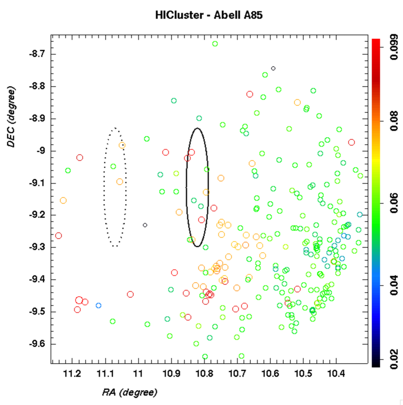
Figure 1: Distribution of optical galaxies in the redshift range $0.02<z<0.1$ around the NRT ON/OFF beam positions near Abell85 cluster in the (RA, DEC) plane. Color scale represents the galaxy redshifts, NRT ON and OFF beam spots are represented as solid and dashed ovals

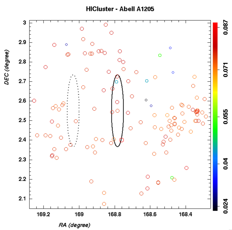
Figure 2: Distribution of optical galaxies in the redshift range $0.02<z<0.1$ around the NRT ON/OFF beam positions near Abell1205 cluster in the (RA, DEC) plane. Color scale represents the galaxy redshifts, NRT ON and OFF beam spots are represented as solid and dashed ovals

3 Data analysis

Two data processing pipelines have been setup to handle data from the BAORadio system, and the standard NRT correlator (ACRT) system, which have similar stages. An overview of the BAORadio pipeline is presented in the next section, followed by the calibration procedure that has been used. Some additional details are given in appendix A, and the ACRT data reduction pipeline is also briefly described in appendix B.

3.1 BAORadio data reduction pipeline

Our data reduction pipeline features the following stages:

1. We first perform an FFT on each digitization frame of 16384 ADC samples, yielding 8192 complex Fourier components, distributed over the $\left[1250,1500\right]\mathrm{MHz}$ total bandwidth. Frequency components have thus a resolution of $\simeq 30.5\leavevmode\nobreak\ \mathrm{kHz}$ or $\simeq 6.4\leavevmode\nobreak\ \mathrm{km/s}$. Each digitization frame and hence each spectrum is time-tagged with $8\leavevmode\nobreak\ \mathrm{ns}$ precision by the ADC-board firmware. However we consider that our absolute time (UT) precision, given by the acquisition computer clock, is around 1-sec. Using the scheduling log files of the NRT operation, these time-tags are used to extract data sets corresponding to different operation sequence of the NRT: diode pulses, focal chariot motion, plane mirror motion … . Notice that these sequences differs for the ”Position-Switching” (PS) observation mode used for the three clusters, or the ”Drift Scan” (DS) mode used for 3C161  (see Sec. 2). As each phase starts with a DAB pulse (see Sec. 3.3) and stops with NRT chariot positioning movement, some margin has been taken to allow for system stabilization, so we use only 30-sec data over the 40-sec available per ON and OFF phases of a cycle.

2. RFI filtering.
   Outside the radio protected band [1400,1427] MHz, many terrestrial signals from communication systems, radars…create spurious signals in the surveyed frequency band [1250,1500] MHz at Nançay. We have used the very fine time sampling of the BAORadio system ($\lesssim 0.1\mathrm{ms}$), to implement an RFI mitigation method for fast intermittent signals, such as radar pulses, using median filtering over time, for each frequency component. Figure 3 shows for instance a time-frequency map, corresponding to $\simeq 86\leavevmode\nobreak\ \mathrm{s}$ observations of Abell85, with $0.6\leavevmode\nobreak\ \mathrm{s}$ time resolution and $\simeq 30.5\leavevmode\nobreak\ \mathrm{kHz}$ frequency resolution. A number of intermittent and permanent RFI signals are clearly visible. We have applied our RFI cleaning method independently to each polarization signal. A more complete description of our RFI mitigation method and corresponding results, applied to each polarization signal $p0,p1$ independently, is given in appendix (A.1).

   

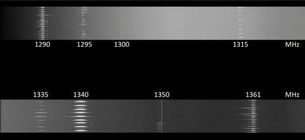
   Figure 3: Time-frequency map of $\simeq 86\mathrm{s}$ observations of Abell85 for one polarization showing intermittent strong radar signals and permanent narrow RFI signals originating from electronic components. The frequency bands covered are $[1285,1325]$ MHz (top) and $[1330,1370]$ MHz (bottom). The other polarization (not shown) experiences the same features

3. Rejection of noisy observations.
   These RFI cleaned spectra are then used to compute average spectra for each DAB, ON, OFF phases of each cycle, for each polarization signal $p0,p1$. These cycle/cycle spectra are then used to produce average spectra over different coarser time scales, per run (observations during a given day), or the whole period. We apply however some additional cuts to delete noisy observations, affected by the Sun transits for instance, or a small fraction of the data affected by electronic instabilities. We find that the BAORadio system associated with the NRT has been quite stable, and reliable; we have been able to keep more than $95\%$ of the whole data sets for all Abell clusters for the final analysis, compared to 50-60% for standard NRT ACRT data (Table 5).

4. Correction to the Local Standard of Rest (LSR) frame.
   For each observation run (day), we have computed the doppler shift due to the movement of the Sun with respect to nearby stars, and corrected the corresponding spectra to obtain spectra in the LSR reference frame. The correction is applied separately for each cycle, polarization ($p=0,1$), and On/Off-source ($s=ON,OFF$) spectra described above. Notice that the frequency shifts are $\lesssim 140\leavevmode\nobreak\ \mathrm{kHz}$, compared to our $30\leavevmode\nobreak\ \mathrm{kHz}$ frequency resolution; we do not do any interpolation along the frequency axis and spectra are only shifted according to an integer rounded number of frequency bins.

5. Computation of the overall frequency response $g(\nu)$.
   The spectral response $g(\nu)$, represents the NRT optics and the BAORadio electronic chain frequency response, although the variations are mainly due to the analog electronic filter shape. We determine a normalized frequency response $g(\nu)$ using measured spectra $P(\nu)$, after filtering and smoothing, so that
   $P(\nu)/g(\nu)\simeq 1$. We have developed two analysis methods, starting from the same set of cycle/cycle spectra, including the frequency response determination $g(\nu)$, adapted for the two calibration methods, using either 3C161  radio source, or the Milky Way 1420 MHz line.
   

   (a) For each cycle, a frequency response function is computed from a smoothed, median filtered version of OFF-source spectra, for each polarization signal
   $g_{0,1}(\nu)=\mathrm{Off}_{filt}$. The final signal toward a given target is obtained by averaging, over all cycles, the difference of ON-source and OFF-source spectra, renormalized by the gain, for each polarization.

   $$\langle\mathrm{(On-Off)/Off_{filt}}\rangle=\left\langle\frac{P_{0,1}^{On}-P_{0,1}^{Off}}{g_{0,1}(\nu)}\right\rangle_{cycles}$$

   (b) Average ON-source and OFF-source spectra are computed for each run (average of all cycles for a given day), and are then used subsequently to compute a normalized frequency response for each run $r$, each polarization $(p=0,1)$, for the ON-source and OFF-source spectra separately $g_{r,(0,1)}^{On,Off}(\nu)$. The average per cycle, per polarization ON/OFF spectra are first filtered with a sliding median filter over a window of $15\,\mathrm{MHz}$ wide, and then modeled as a spline curve with $4\,\mathrm{MHz}$ step. The smooth spline frequency responses $g_{r,(0,1)}^{On,Off}(\nu)$ are free from RFI and are used to correct the original ON/OFF-source spectra, for each run and polarization. The final signal toward each observed ON-source and OFF-source is then computed by averaging the normalized gain corrected spectra from each observation run:

   $$\langle\mathrm{On/g_{On}}\rangle = \langle P_{0,1}^{On}(\nu)\,/\,g_{r,(0,1)}^{On}(\nu)\rangle_{runs}$$

   $$\langle\mathrm{Off/g_{Off}}\rangle = \langle P_{0,1}^{Off}(\nu)\,/\,g_{r,(0,1)}^{Off}(\nu)\rangle_{runs}$$

6. Radiometric calibration.
   The final average spectra obtained in the previous step are not expressed in physical units, but in r.a.u (Relative Arbitrary Unit). The conversion factor into physical units, brightness temperature (Kelvin) or source intensity (Jansky) is determined using the 3C161  source for the (a) $\langle\mathrm{(On-Off)/Off_{filt}}\rangle$ spectra and the Milky Way 1420 MHz line for (b) $\langle\mathrm{On/g_{On,Off}}\rangle$. The calibration procedure is described in next section.

We obtain fully compatible final spectra, using the two methods (a), (b) described above to determine frequency response and compute radiometric calibration coefficients. This will be discussed further in Sec. 4.

3.2 Residual modulations in the final spectra

We observe residual structures in the ON-source or OFF-source spectra, independent of the processing method used (a) or (b). As shown in Fig. 5 we have observed two regimes of modulation of the spectra. The first one, with a particularly unexpected large amplitude of $\gtrsim 100\leavevmode\nobreak\ \mathrm{mJy}$, has a modulation period in frequency of about $3-4\,\mathrm{MHz}$. It is attributed to standing waves in the $\simeq 25\leavevmode\nobreak\ \mathrm{m}$-long cables connecting NRT front-end electronics and the BAORadio analog chain, combined with a slight impedance mismatch in the BAORadio analog electronic input stage. The second one, smaller in amplitude with $\simeq 500\,\mathrm{kHz}$ period structures in frequency, (see zoom in Fig. 5) is attributed to the standing waves between the large spherical mirror and the horn, located $\simeq 280\leavevmode\nobreak\ \mathrm{m}$ north of the spherical mirror. Notice that this last modulation had suffered from a sudden $\pi/2$ phase shift during a period of cycles. Unfortunately both kind of modulations not only are non uniform on the total 250 MHz bandwidth but also are time varying. Different kind of filtering have been tried to analyze the ON or OFF spectra alone without any success and it is the reason why we have used (ON-OFF) spectra which reduce considerably these modulations as one can appreciate looking at cyan versus blue spectra in Fig. 5.

3.3 Radiometric calibration

The standard procedure provided by the NRT for calibration is based on the use of noise diodes (DAB) signal injected at the horn level. Initially, we followed the NRT procedure for relative calibration using the DAB signals, but we have shown that this method induces additional instabilities, leading to a significant increase of the final signal fluctuations or noise level. Figure 5 shows the increase of fluctuations where DAB signal is used for relative cycle/cycle signal level calibration. The same effect is observed for the NRT ACRT signal and discussed in appendix B.4. We have found that the NRT and BAORadio chains are quite stable, even over durations of a few months, and we have only used the radiometric sources and the Milky Way $\mathrm{H_{I}}$ line to determine the absolute calibration.

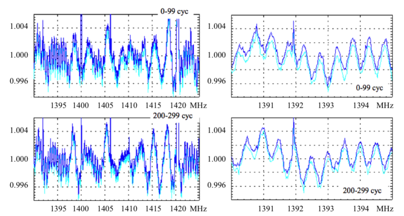
Figure 4: Left panels: cumulated On/Off_filt (cyan) and Off/Off_filt (blue) for polarization p0, segmented into two periods of 99 cycles from the observations of Abell1205. Clear modulations of the spectra are visible with a frequency of the order of 3-4 MHz. Right panels: a zoom of the left panels clearly shows 500 kHz modulation. Notice that between the two right panels the modulation phase has changed by $\pi/2$

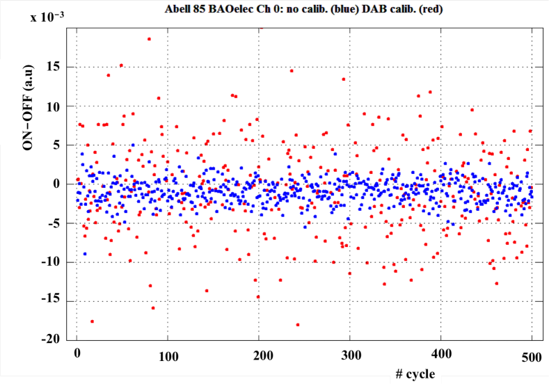
Figure 5: Distributions of the difference of power (ON-OFF) integrated in the frequency band $[1420.2,1420.6]$MHz (arbitrary unit) around the Milky Way $\mathrm{H_{I}}$ line for one polarization (polar. 0) given by the BAORadio system. The blue dots are obtained with no calibration applied while the red dots show the effect of the DAB calibration applied for each cycle (ON, OFF). The use of the DAB calibration increases the sigma of the ON-OFF by a factor approximatively $2.5$

3.3.1 Radiometric calibration using 3C161

The radio-continuum source 3C161  has been observed in drift scan mode. During the entire observation time, we have registered several 3C161  transits with both polarizations. The average of the different transits is shown in Fig. 7.

We have derived the absolute radiometric calibration coefficient $C_{a}$ for the average spectra
$\langle\mathrm{(On-Off)/Off_{filt}}\rangle$ by comparing the peak value of 3C161  transit, after baseline subtraction, averaged over the 2 polarizations, to the published emission intensity measurement for 3C161  (Ott et al.,, 1994; Baars et al.,, 1977) of $18.58\pm 0.09$ Jy for the continuum flux collected by a circularly-polarized total power receiver centered at 1408 MHz, with a 20 MHz bandwidth ([1398, 1418] MHz). The quoted error is a systematic error reflecting the 3% difference between the two referenced measurements. It yields

$$C_{a}=22.6\pm 0.6\,\mathrm{Jy/r.a.u}$$

The radiometrically calibrated spectra in Jansky corresponding to the difference of ON-source, OFF-source for each cluster are obtained by multiplying the average of the two polarizations by $C_{a}$:

$$S(\nu)=\frac{C_{a}}{2}\left(\langle\mathrm{(On-Off)/Off_{filt}}\rangle_{p0}+\langle\mathrm{(On-Off)/Off_{filt}}\rangle_{p1}\right)$$

Using the spectral fit of reference Ott et al., (1994), we have determined the $C_{a}$ coefficients for the frequency band covered by the three Abell clusters. The coefficient is constant at a few percent level, we are thus confident that our 3C161  calibration method is valid indeed for the whole frequency band needed to search for $\mathrm{H_{I}}$ emission line (Sec. 4.2).

The above value of the derived calibration coefficient has also been checked using the $\mathrm{H_{I}}$ source NGC4383. See the appendix for more details.

3.3.2 Radiometric calibration using Milky Way 1420 MHz line

The frequency band observed contains the Milky Way $\mathrm{H_{I}}$ emission line at 1420 MHz. Using the ON-source and OFF-source observations separately we have identified the Milky Way emission line, corrected from Doppler shift (i.e. LSR correction), and compared its strength to the Leiden/Argentine/Bonn (LAB) Survey of Galactic $\mathrm{H_{I}}$ database (Kalberla et al.,, 2005). This procedure is indeed quite difficult as the ON and OFF spectra are affected in a similar way by the residual structures in the spectra (see Sec. 3.2). To minimize the impact of these residual structure, we have performed a spline modeling of the base line, before extracting the Milky Way emission line strength from our ON,OFF-source spectra. Notice that the $\langle\mathrm{(On-Off)/Off}_{filt}\rangle$ spectra obtained with the (a) method, computed cycle by cycle automatically cancel the above mentioned artifacts. We have also checked that the temperature measured by the LAB survey doesn’t vary significantly in the NRT beam. The LAB survey measurement are expressed as brightness temperature, so we have used the standard NRT antenna temperature $T_{a}$ to point source intensity $I_{s}$ conversion factor, as given by the NRT point source efficiency of $\eta=0.56$ and a collection area $A=200\times 35=7000\mathrm{m^{2}}$ (Gérard E., private communication). It yields

$$2\,k_{B}\,T_{a}=\eta\,A\,I_{s}\hskip 8.53581pt\rightarrow\frac{T_{a}}{I_{s}}=\frac{\eta\,A}{2k_{B}}=1.42\,\mathrm{K/Jy}$$

We have computed an absolute radiometric calibration coefficient $C_{b}$, for each polarization signal, each observation run (day) and ON-source, OFF-source spectra, and for each observed cluster. The calibration is rather stable: the figure 7 shows the variation of the Abell85 calibration coefficients for the $32$ runs over a $4$ months period from April to October 2011. The derived value of the calibration coefficient, with a systematic error of 5-10 %, and statistical error of a few percent:

$$C_{b}\simeq 20\pm 2\,\mathrm{Jy/r.a.u}$$

is compatible with the $C_{a}$ coefficient obtained from the 3C161  source.

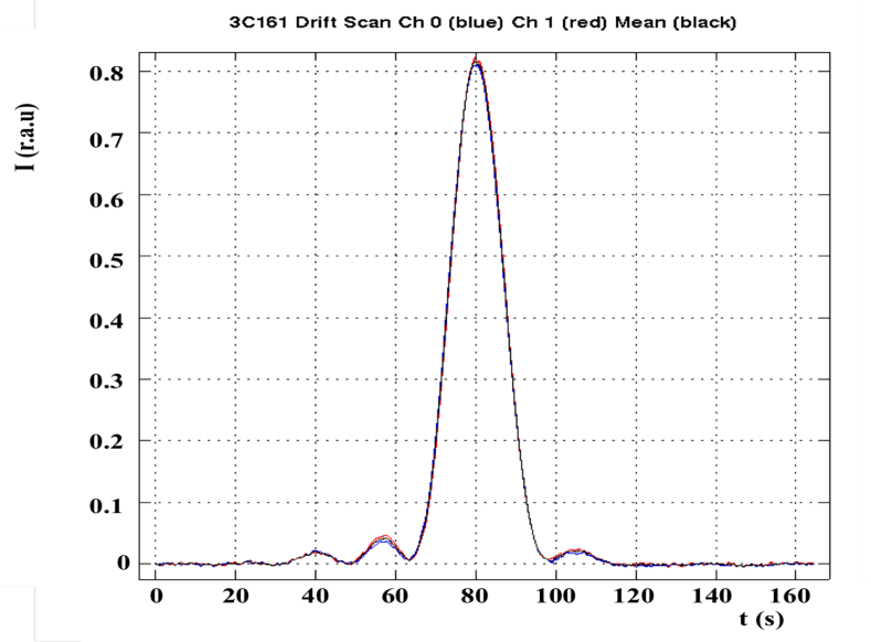
Figure 6: BAORadio mean $\langle\mathrm{(On-Off)/Off}_{filt}\rangle$ integrated in the [1412, 1413] MHz band averaged over the transits of 3C161  observation. Both polarization channels (red/blue) as well as their mean value (black) are displayed

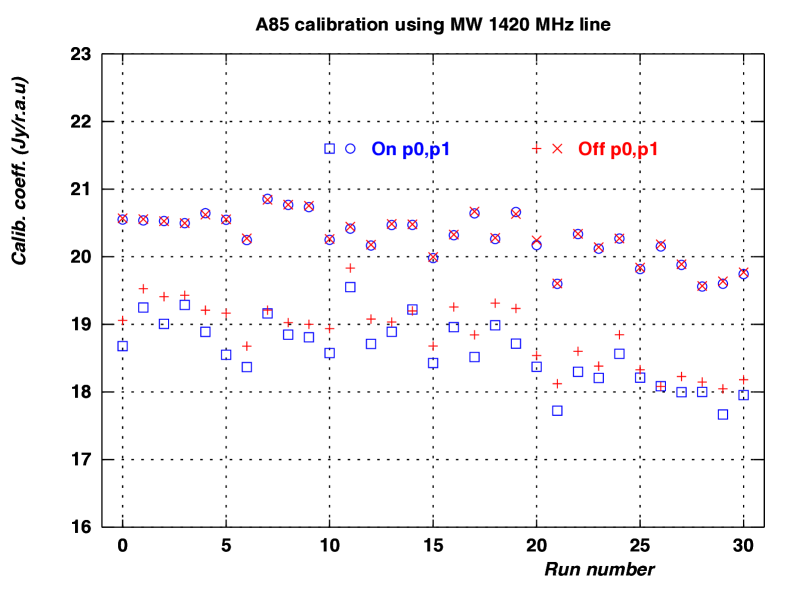
Figure 7: variation of the Abell85 calibration coefficients for the $32$ used observation runs. Blue squares and circles corresponds to the two polarizations ($0,1$) and the ON-source pointings, while red plus and cross markers corresponds to the OFF-source pointings

4 Results

4.1 Sensitivity as a function of integration time

For each cluster observation, we have applied the RFI filtering and data cleaning procedures exposed in previous sections, then we have used the time series of $\langle\mathrm{(On-Off)/Off}_{filt}\rangle$ spectra integrated over 1 MHz around the ACRT observation frequency (Table 1) to draw for both ACRT and BAORadio systems the evolution of the fluctuation R.M.S as function of the integration time, the so-called radiometer curve (details on the ACRT data analysis are in Sec. B). To compare the two systems, we have defined an ”effective integration time” taking into account the difference of useful fraction of time ON-sky observation: 100% for ACRT and 25% for BAORadio. The result is shown in Fig. 8 for BAORadio (reap. ACRT): Abell1205 in blue (red) around 1321 MHz, Abell85 in green (brown) around 1346 MHz and Abell2440 in purple (orange) around 1302 MHz. The blue solid line represents the expected curve for a system affected only by white noise. The red line of Fig. 17 (top) represents the curve obtained for all clusters with ACRT data analyzed with NRT standard NAPS pipeline (Renaud,, 2007).

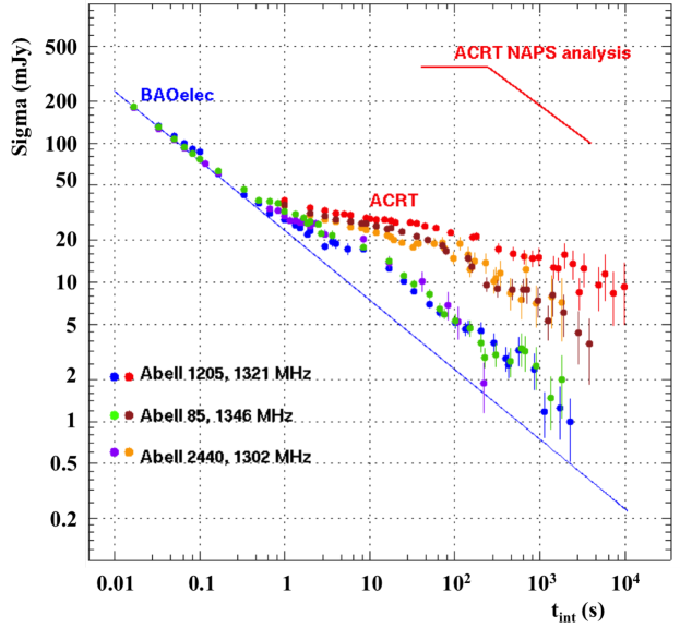
Figure 8: Radiometer curve, sigma of the mean of the two polarization signals averaged over 1 MHz around the central frequency observed in ACRT versus integration time, obtained for BAORadio (ACRT) data for the three clusters: Abell1205 in blue (red) around 1321 MHz, Abell85 in green (brown) around 1346 MHz and Abell2440 in purple (orange) around 1302 MHz. The blue solid line represents the expected curve for a system affected only by white noise. The red line represents the curve obtained for all clusters with ACRT data analyzed with the NRT standard pipeline. The sigma of the last points are estimated with 5 samples of the quoted integration time. The total statistics on each Abell cluster are quoted in Table 5

The ACRT data has been processed down to its minimum integration time of 1-sec. For BAORadio, we have processed part of the data down to 16.7 ms integration time and the whole data set at 8.4 sec. In the range of integration time greater than 1-sec, the ACRT sigma is larger by factor two than the BAORadio one. Moreover the ACRT sigma evolution differs from a white noise trend which is a sign of additional noises present in the integrated $\langle\mathrm{(On-Off)/Off}_{filt}\rangle$ in the frequency band of interest. This is due to both differences between ON and OFF power levels within the same cycle and from cycle to cycle variations. Notice that our ACRT pipeline gives notably better results than the standard NAPS pipeline, when we consider the total power evolution during cycles, as shown in Fig. 17 (top).

For BAORadio the radiometer curve is similar to a pure white noise below 1-sec and remains lower than the ACRT curve for greater integration times. One possible origin of the ”1-sec” trend change is the noise generated by the 1-sec duty cycle of the cryogenic cooling system for the low noise amplifier in the chariot.

Figure 9 shows the fluctuation or noise level for the $\mathrm{\langle On/g_{on}-Off/g_{off}\rangle}$ spectra calibrated using the Milky Way 21 cm emission. The noise level has been computed as the standard deviation ($\sigma$) along the frequencies, in a $16\,\mathrm{bins}$ or $\Delta\nu=488\mathrm{kHz}$ wide sliding window. Although the corresponding figure for the 3C161  calibrated $\langle\mathrm{(On-Off)/Off}_{filt}\rangle$ is not shown, we obtain very similar values for the fluctuation level, over the full frequency band. This is an additional indication that the calibration procedures described in Sec. 3.3 and Sec. 3.3.1 are compatible.

The noise level is nearly flat for most of the frequency band $[1300,1430]\leavevmode\nobreak\ \mathrm{MHz}$, with single polarization noise level $\sigma_{1pol}\lesssim 4\,\mathrm{mJy}$ for Abell85, and $\sigma_{1pol}\lesssim\,2.75\mathrm{mJy}$ for Abell1205. There are however few narrow frequency bands where the fluctuations are significantly higher around $\nu\simeq 1313$, 1329, 1356, 1376, 1382, 1386, 1402$\leavevmode\nobreak\ \mathrm{MHz}$. In the following section, we will use $\sigma_{A85}\simeq 2.7\mathrm{mJy}$ and $\sigma_{A1205}\simeq 1.8\mathrm{mJy}$ for the signal corresponding to the average of the two polarizations $s(\nu)=(p0+p1)/2$, for a single frequency bin ($\simeq 30.5\leavevmode\nobreak\ \mathrm{kHz}$), for Abell85 and Abell1205 respectively. This noise level is compatible with the one shown in Fig. 8.

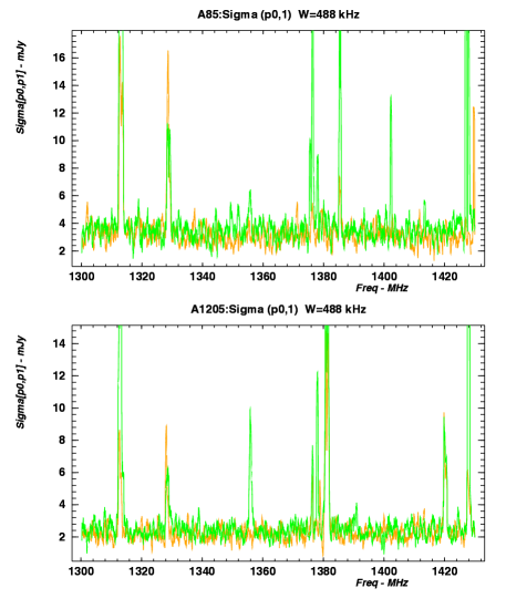
Figure 9: Noise level (fluctuations) in mJy as a function of frequency for both polarizations, estimated from the standard deviation (sigma) along the frequency, using a 488 kHz sliding window over the normalized $\mathrm{\langle On/g_{on}-Off/g_{off}\rangle}$ spectra calibrated using the Milky Way 21 cm emission from the full Abell85 and Abell1205 data sets. Similar results have been obtained with the 3C161  calibrated $\langle\mathrm{(On-Off)/Off}_{filt}\rangle$ spectra over the full frequency band

The expected noise level in $\mathrm{mJy}$ for the sum of the two polarization signal, for an instrument characterized by a collecting area $A$ and efficiency $\eta$, a system temperature $T_{sys}$, total integration time $t_{int}$ and bandwidth $\delta\nu$ can be written as:

$$\sigma^{2pol}=10^{29}\times\frac{\sqrt{2}\,k_{B}\,T_{sys}}{\eta A\,\sqrt{t_{int}\times\delta\nu}}\hskip 14.22636pt\mathrm{mJy}$$

Assuming a value of the system temperature $T_{sys}\simeq 35\leavevmode\nobreak\ \mathrm{K}$ for NRT, a collecting area $A=7000\,\mathrm{m^{2}}$, a point source efficiency of $\eta\simeq 0.56$ and a frequency bandwidth $\delta\nu=30.5\mathrm{kHz}$ corresponding to the BAORadio spectral resolution, we obtain:

$$\sigma^{2pol}(t_{int})\simeq\frac{100}{\sqrt{t_{int}}}\hskip 5.69054pt\mathrm{mJy}$$

The expected noise level would then be $\sigma^{2pol}\simeq 2\mathrm{mJy}$ for $t_{int}=2000\leavevmode\nobreak\ s$ integration time in good agreement with measured values from our analysis pipeline by the two calibration methods (Sec. 3.3 and Sec. 3.3.1). Moreover, this result presented here toward the three targets in three different frequency bands suggests that BAORadio system and analysis pipeline is robust over a large frequency domain.

4.2 $\mathrm{H_{I}}$ signal search

The standard procedure to process ACRT data, in case of known line search, is to make a polynomial baseline fit on $\langle\mathrm{(On-Off)/Off}_{filt}\rangle$ spectra, which allows suppressing the global offset due to gain variations and the oscillation residuals in the spectrum before calculating the fluctuation dispersion. Of course, the line which is searched for in the spectrum is masked to protect it from suppression, hence it is necessary to know precisely both its frequency and width.

In the analysis presented here we do not have precise information about the $\mathrm{H_{I}}$ signals we are searching for in the clusters. In the $\mathrm{H_{I}}$ intensity mapping this would be even more true as individual galaxy emission would not be significant. Given the NRT beam width, the confusion also increases quickly with redshift. In the case of the observed targets here, and as it can be seen in Figs. 2 and 2, several possible $\mathrm{H_{I}}$ lines might be present in a narrow (few MHz) frequency band. Some of them are emission lines due to galaxies in the On beam while others are looking like absorption lines due to galaxies in the OFF beam.

We have searched for extra power above the noise level around each cluster redshift frequency (Table 1) using data from the BAORadio system which is more sensitive than ACRT system. We have performed the cluster signal search using the $\mathrm{\langle On-Off\rangle/Off_{filt}\rangle}$ spectra calibrated by the 3C161  analysis, as well as
$\mathrm{\langle On/g_{on}-Off/g_{off}\rangle}$ spectra calibrated using the Milky Way $\mathrm{H_{I}}$ line (Sec. 3.3). Both sets of spectra have been Doppler shift corrected. We obtain compatible results for the $\mathrm{H_{I}}$ emission from Abell85 and Abell1205 using both sets of spectra. For the sake of clarity, we present here only the analysis of the $s(\nu)=\mathrm{\langle On/g_{on}-Off/g_{off}\rangle}$ spectra, as this second method insures that the average signal is zero, making the search for emission or absorption lines easier.

Table 2: List of frequency peaks above $\pm 1\sigma$ in the Sum spectrum of Fig. 10 and the result of investigation of possible origin of these extra power emission during our observation

Frequency	Comments
1332.0 MHz	the peak has been found as a RFI occurring one day
1336.6 MHz	the peak is due to radar tail emission
1350.0 MHz	at this frequency there is a strong radar emission line
	and we have also a well identify electronic noise
1353.0 MHz	no human RFI emission found responsible of this peak
1361.3 MHz	the same kind of radar tail emission as 1336.6 Mhz

The spectra from the mean of two polarization channels (i.e. $(p_{0}+p_{1})/2$) averaged over a sliding window of size $16\,\mathrm{bins}$ or $\Delta\nu=488\leavevmode\nobreak\ \mathrm{kHz}$ from Abell85 and Abell1205 data are shown on the figure 10 below. Frequency components exhibiting large fluctuations as can be seen for instance in Fig. 9 were excluded when computing the average power in the $488\leavevmode\nobreak\ \mathrm{kHz}$ sliding window. Notice that the displayed points are separated by 124 kHz, and the vertical scales differ on the right and left hand side plots. As expected, the fluctuations are smaller for Abell1205 compared to Abell85 given the longer integration time and lower noise level. The 40 MHz wide frequency range around the Abell85 cluster $[1330,1370]\leavevmode\nobreak\ \mathrm{MHz}$ is represented on the right hand side of Fig. 10, while the plots on the left side show the 40 MHz frequency band centered on Abell1205 $[1300,1340]\leavevmode\nobreak\ \mathrm{MHz}$.

The signal we are searching for is unpolarized while RFI will appear often more strongly in one linear polarization. The difference of the two polarizations signal is also shown on the above mentioned figure (red triangles) and should be compatible with zero for an $\mathrm{H_{I}}$ signal. We have also represented the +3 sigma detection threshold for Abell85 and Abell1205 based on the noise levels determined in Section 4.1, taking into account the sliding window size.

We have investigated possible terrestrial origins for extra power emission in the frequency bands around Abell85, Abell1205 redshifts and for instance the corresponding results for Abell85 are summarized in Table 2. We have also searched in the frequency range $[1330,1370]$ MHz for possible RFI emissions responsible for the emission in the data taken during Abell1205 and Abell2440 observations as the three clusters have been observed during the same period.

As already mentioned, Abell1205 data have a lower noise level, due to a larger total integration time. Comparing Abell85 and Abell1205 spectrum around 1350 MHz (Fig. 10), Abell1205 spectrum does not show any extra power around the central frequency, while emissions with statistical significance exceeding 3 sigma are observed around 1350 MHz and 1353 MHz in the Abell85 spectrum. The origin of the observed emission around 1350 MHz can not be unambiguously attributed to emission from galaxies in the beam. Indeed, we have identified intermittent radar emission at 1350 MHz, and although no emission is detected at or near 1350 MHz in the Abell1205 spectrum, we do observe signs of polarized RFI close to this frequency in the Abell2440 spectrum. On the other hand, we have not found any suspect sporadic emission in our data as well as known RFI emission around 1353 MHz. We consider thus that we have detected $\mathrm{H_{I}}$ emission from galaxies belonging to Abell85 at 99% confidence level.

We also have searched for extragalactic $\mathrm{H_{I}}$ emission in the Abell1205 spectrum, around 1320 MHz, corresponding 1420 MHz line shifted according to this cluster redshift ($z\simeq 0.077$). Comparing the Abell1205 and Abell85 data around this frequency (see Fig. 10), we observe no significant feature in the Abell85, while we observe an excess power in the frequency band $[1315,1320]\leavevmode\nobreak\ \mathrm{MHz}$, and an even narrower feature exceeding marginally the 3-sigma threshold around 1318 MHz. A small frequency band below 1315 MHz were subject to RFI and has been blanked. Although the statistical significance is weaker than the Abell85, we consider that we have also detected $\mathrm{H_{I}}$ emission from Abell1205 at 1318 MHz.

We do not show the Abell2440 spectrum as the corresponding observation time represent less than 1/3 of the time spent on Abell85 and as the frequencies corresponding to Abell2440 redshift ($z\simeq 0.092,\nu_{0}\simeq 1302\mathrm{MHz}$) are affected by strong RFI (1292 MHz, and 1301 MHz).

Compared to previous $\mathrm{H_{I}}$ surveys with the NRT (van Driel et al.,, 2001; Pustilnik et al.,, 2002; Monnier Ragaigne et al.,, 2003), our detection threshold and line strength sensitivities have been lowered by a factor $\simeq 5$, from $\simeq 2\,\mathrm{Jy\,km/s}$ to $\simeq 0.4\,\mathrm{Jy\,km/s}$, for comparable, total integration times ($1\div 3$ hours per target). One can notice also that the achieved sensitivity limits, in term of line strength $P^{*}_{21}$ (Table LABEL:Tab:expected-signal) is comparable to the one obtained by the AGES survey toward Abell1367 (Cortese et al.,, 2008).

A more in depth analysis of the observed signals toward Abell85 and Abell1205, and corresponding $\mathrm{H_{I}}$ mass estimates are presented in the next section.

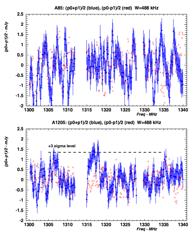
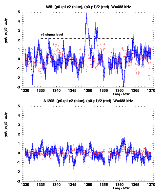
Figure 10: Sum (blue circles) and Difference (red triangles) (in mJy) of the two polarization signals integrated over a 488 kHz wide sliding window for the Abell85 (top) and Abell1205 (bottom), The represented points are separated by 124 kHz. Left: the 40 MHz wide frequency band centered around Abell1205 redshift ($z\simeq 0.08,1320\leavevmode\nobreak\ \mathrm{MHz}$). Right: The 40 MHz wide frequency band, centered around Abell85 redshift ($z\simeq 0.05,1350\mathrm{MHz}$). Notice that the vertical scale is different for the left and right hand set of plots

5 Interpretation, discussion

Using the NED extragalactic database and SDSS DR10 data sets, we have identified galaxies in the NRT beam, around the ON source and OFF source pointing of the telescope for the two targets and in the redshift range ($z\lesssim 0.1$) covered by our observations. The spatial distribution of galaxies, with color coded redshift around the NRT targets in Abell85 and Abell1205 are shown in Figs. 2 and 2.

We have also computed the expected signal strength $P_{21}$ from $\mathrm{H_{I}}$ emission in galaxies at the distance of observed clusters using the following formula and luminosity distance to the clusters:

$$P_{21}=2.4\,\,10^{18}\,\frac{M_{\mathrm{H_{I}}}}{M_{\odot}}\,\,\mathrm{W}$$

The results are summarized in the table shown on the right.

Expected total signal strength $P_{21}^{*}$ received on Earth, from 21 cm emission of a total $\mathrm{H_{I}}$ mass of $10^{10}$ $\mathrm{M_{\odot}}$ at the three cluster distances studied here. $P_{21}^{*}$ is given in $\mathrm{Jy\,km/s}$ and $\mathrm{mJy.MHz}$ in brackets
$\nu\,(\mathrm{MHz})$ $z$ $d_{L}\,(\mathrm{Mpc})$ $P_{21}^{*}$ Abell85 1353 0.0498 228 0.830   (3.86) Abell1205 1318 0.0777 363 0.326   (1.52)

The galaxies with redshift measurements have been extracted from the NED database around the ON and OFF positions of the NRT beam toward Abell85 and Abell1205. Then, these galaxies were cross matched with SDSS-DR10 galaxies with photometric or spectroscopic redshifts. The list of galaxies relevant for the study discussed here is presented in Table 3. Assuming a gaussian beam shape for the NRT, we have kept galaxies up to a maximum distance of 2-sigma from the beam center. We have also applied a selection cut on the redshift, such as the redshifted $\mathrm{H_{I}}$ emission frequency falls in the 20 MHz wide frequency band $1342<\nu<1362\,\mathrm{MHz}$ for Abell85, and $1311<\nu<1333\,\mathrm{MHz}$ for Abell1205. We have checked the list of galaxies using the SDSS-DR10 database of galaxies with photometric redshifts, and we have added one galaxy to the Abell85-On list, which seemed relevant to the study here. In total, we have kept 8, respectively 11 galaxies for the Abell85, resp. Abell1205 ON-source position, 1 and 4 objects for the corresponding OFF-source positions. In addition to object position J2000 (RA, DEC), NED magnitude and redshift, we have listed the NRT relative beam efficiency toward the source $\eta_{r}$, assuming a gaussian beam profile $4^{\prime}\times 22^{\prime}$, and the SDSS g,r band magnitudes whenever possible.

The signal spectrum we have obtained toward Abell85 and Abell1205 have a low signal to noise ratio. We have however tried to fit line shapes for multiple sources to our measured spectra. The $\mathrm{H_{I}}$ line shape and width depends on the galaxy type, mass and viewing angle. Given our low S/N spectra, we have modeled the emission line profiles as gaussians. The non linear fit procedure determined the gaussian positions (central frequency) and amplitudes, as well as an overall mean signal level assuming line widths. However, approximate best values for these line widths has been obtained through an iterative fitting. The FWHM line widths that we have obtained range from 380 to 550 kHz (80 - 120 km/s), although weakly constrained.

Table 3: List of galaxies in the NRT ON/OFF beam observed toward Abell85 (first table) and Abell1205 (second table), extracted from the NED database, identified as galaxies with redshift measurement. In each table, the first list, galaxies numbered with (+) superscript correspond to the galaxies in the ON beam, while the second list with (-) superscript, corresponds to galaxies in the OFF Beam. mag is the magnitude by the NED database, while magg, magr are the SDSS DR10 magnitudes in the g,r bands, for the associated SDSS source. $\eta_{r}$ is NRT relative beam efficiency towards the source, assuming a gaussian beam with FWHM equal to 4’ in RA, 22’ in DEC. Sources marked as Pz are extracted from SDSS DR10 galaxy tables with photometric redshifts

Galaxy label	Obj. Name	RA (deg)	DEC (deg)	redshift	mag	$\nu$	magg	magr	$\eta_{r}$
Abell85
G1(+)	2MASX J00431039-0903243	10.7934	-9.0569	0.0578	16.40	1342.81	16.3	15.5	0.60
G2(+)	SDSS J004310.94-092239.7	10.7956	-9.37772	0.0559	18.46	1345.18	18.9	18.1	0.17
G3(+)	SDSS J004322.80-091635.0	10.8450	-9.27641	0.0539	18.91	1347.72	19.3	18.6	0.42
G4(+)	SDSS J004310.95-091800.3	10.7957	-9.30009	0.0532	18.62	1348.67	18.7	18.2	0.34
G5(+)	SDSS J004319.53-090912.9	10.8314	-9.1536	0.0502	19.15	1352.46	19.5	19.1	0.91
G6(+)	SDSS J004314.35-091021.3	10.8098	-9.17261	0.0501	18.37	1352.65	18.9	18.6	0.87
G7(+)	GALEXASC J004315.79-085355.1	10.8160	-8.89925	0.0497	19.04	1353.17	-	-	0.40
G8(+) (Pz)	SDSS (Photo-z)	10.8127	-9.06866	$0.051\pm 0.017$	-	1351.40	19.5	19.4	0.92
G9(-)	2MASX J00441835-0902545	11.0764	-9.04854	0.0574	17.4	1343.34	17.2	16.3	0.90
Abell1205
G11(+)	SDSS J111500.29+024756.7	168.751	2.79908	0.0799	18.5	1315.33	18.5	17.8	0.15
G12(+)	SDSS J111505.42+024835.7	168.773	2.80994	0.0795	18.3	1315.79	18.3	17.5	0.24
G13(+)	2MASX J11150889+0235435	168.787	2.59539	0.0794	17.9	1315.88	18.1	17.1	0.96
G14(+)	SDSS J111505.17+025118.8	168.772	2.85524	0.0793	17.7	1316.07	17.8	17.3	0.14
G15(+)	2MASX J11150843+0243335	168.785	2.72596	0.0785	16.8	1317.06	16.8	16.2	0.54
G16(+)	2MASX J11151499+0239533	168.812	2.66472	0.0783	17.7	1317.21	-	-	0.49
G17(+)	2MASX J11151546+0232363	168.814	2.54348	0.0779	17.2	1317.76	17.1	16.1	0.59
G18(+)	WISEPC J111459.91+024551.0	168.750	2.76446	0.0765	17.4	1319.45	17.5	17.4	0.19
G19(+)	SDSS J111516.72+022308.7	168.820	2.38577	0.0764	18.2	1319.63	18.3	17.5	0.28
G20(+)	SDSS J111508.37+023301.4	168.785	2.55039	0.0761	18.2	1319.95	18.2	17.8	1.00
G21(+)	2MASX J11151316+0224125	168.805	2.40360	0.0731	17.6	1323.67	17.5	16.6	0.52
G22(-)	SDSS J111611.93+022237.1	169.050	2.37700	0.0768	18.0	1319.08	18.0	17.4	0.48
G23(-)	SDSS J111604.50+022946.6	169.019	2.49630	0.0763	18.2	1319.68	18.1	17.1	0.81
G24(-)	2MASX J11161766+0221129	169.074	2.35358	0.0763	17.3	1319.68	17.5	16.8	0.19
G25(-)	2MASX J11162139+0235209	169.089	2.58901	0.0742	18.7	1322.25	17.2	16.2	0.17

We have modeled the Abell85 spectrum in the frequency range as a sum of $n=5$ gaussian profiles, plus a constant in the frequency range $1344-1358\,\mathrm{MHz}$, while the Abell1205 spectrum in the frequency range $1310-1324\,\mathrm{MHz}$ has been modeled as a sum of $n=9$ gaussian profiles, plus a constant term. It yields

$$s(\nu)=C+\sum_{i=1}^{n}\,A_{i}\,\exp\left(-\frac{(\nu-\nu_{i})^{2}}{2\sigma_{i}^{2}}\right)$$

The fit results for the Abell85 and Abell1205 are presented in Table 4 and shown in Fig. 11. The fit has been performed on the unbinned spectrum, the fitted model represented as the solid black line, and the measured spectra, averaged over 244 kHz wide window represented as blue circles with error bars.

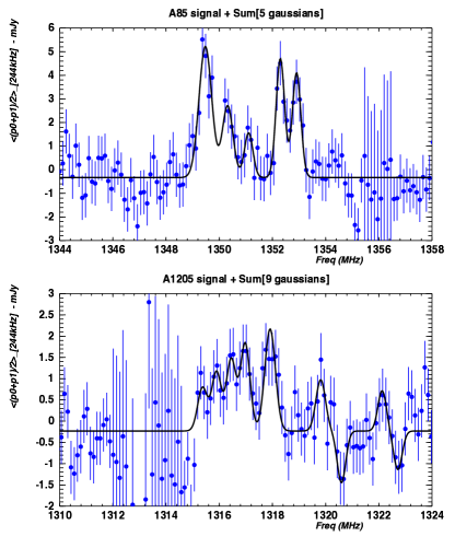
Figure 11: Result of the fit of the $\mathrm{H_{I}}$ signal modeled as a sum of 5 gaussian profiles for Abell85 (top), in the frequency range $[1344,1358]\mathrm{MHz}$ and as a sum of 9 gaussian profiles for Abell1205 (bottom), in the frequency range $[1310,1324]\mathrm{MHz}$. The curve (black line) represents the fit result, and blue circles the actual measurements, sum of the two polarization measurements, averaged over 244 kHz (8 frequency bins). We have represented one point every 122 kHz (4 frequency bins) and error bars are derived from the fluctuations computed along the frequency axis (see Fig. 9)

Abell85:

1. We have no galaxy in our list (see Table 3) that could be associated to the two emission lines L1, L2 at 1349.48 and 1350.3 MHz. As mentioned in the previous section, these two emission like features might be due to imperfectly cleaned RFI.

2. The 1.9 mJy line L3 at 1351.1 MHz might be associated with the galaxy labeled $G8$ in the Abell85 list. Assuming $\eta\simeq 0.9$, the estimated $\mathrm{H_{I}}$ mass would be :

   $$L3:\hskip 2.84526ptM_{\mathrm{H_{I}}}\simeq 2.3\pm 1\times 10^{9}\,M_{\odot}\hskip 5.69054pt(V_{HI}=14625\pm 20\,\mathrm{km/s})$$

3. The two lines L4, L5 at 1352.3 , 1352.9 MHz are probably associated with the galaxies labeled $G5,G6,G7$. Assuming $\eta\simeq 0.9$ for L4 and $\eta\simeq 0.4$ for L5, we obtain the following $\mathrm{H_{I}}$ mass estimates:

   $$L4:\hskip 2.84526ptM_{\mathrm{H_{I}}}\simeq 5.6\pm 1.4\times 10^{9}\,M_{\odot}\hskip 5.69054pt(V_{HI}=14375\pm 20\,\mathrm{km/s})$$

   $$L5:\hskip 2.84526ptM_{\mathrm{H_{I}}}\simeq 1.1\pm 0.3\times 10^{10}\,M_{\odot}\hskip 5.69054pt(V_{HI}=14245\pm 10\,\mathrm{km/s})$$

Abell1205:

1. The first three lines L11-L13 (at 1315.4. 1315.9, 1316.5 MHz) might be associated with galaxies labeled $G11$ to $G14$ in Abell1205 galaxy list. The total associated neutral hydrogen mass would be $M_{\mathrm{H_{I}}}\simeq 12.\times 10^{9}\,M_{\odot}$ , for $\eta\simeq 1$.

2. The line L14 at 1317 MHz can be associated to the Abell1205 galaxies labeled $G15,G16$, while the line L15 at 1317.9 MHz is likely to be due to the G17 galaxy. Assuming $\eta\simeq 0.6$, we obtain the associated neutral hydrogen masses :

   $$L14:\hskip 2.84526ptM_{\mathrm{H_{I}}}\simeq 10\pm 3\times 10^{9}\,M_{\odot}\hskip 5.69054pt(V_{HI}=21825\pm 20\,\mathrm{km/s})$$

   $$L15:\hskip 2.84526ptM_{\mathrm{H_{I}}}\simeq 13\pm 3\times 10^{9}\,M_{\odot}\hskip 5.69054pt\hskip 5.69054pt(V_{HI}=21635\pm 20\,\mathrm{km/s})$$

3. The fitted line L16 at 1319.8 MHz is probably associated with the Abell1205 galaxies labeled $G18,G19,G20$, with a total hydrogen mass of $M_{\mathrm{H_{I}}}\simeq 3\pm 1.5\times 10^{9}\,M_{\odot}$ with $\eta\simeq 1$.

4. The other fitted lines (L17, L18, L19) cannot be associated to our knowledge to galaxies in the ON or OFF beam although the Table 3 might be incomplet.

Integrating simply the Abell85 spectrum in the frequency band $\nu\in[1351,1353]$ will yield a total $\mathrm{H_{I}}$ brightness of $P_{21}^{*}\simeq 0.75\,\mathrm{Jy\,km/s}$, corresponding to a total mass of $M_{\mathrm{H_{I}}}\simeq 1.5\,10^{10}\,M_{\odot}$ for $\eta\simeq 0.6$, while performing a similar integration on the Abell1205 spectrum in the frequency band $\nu\in[1315,1318.5]$ will yield a total $\mathrm{H_{I}}$ brightness of $P_{21}^{*}\simeq 0.65\,\mathrm{Jy\,km/s}$ corresponding to a total hydrogen mass $M_{\mathrm{H_{I}}}\simeq 3.3\,10^{10}\,M_{\odot}$. These values are in agreement with the ones given above. It should also be noted that the quoted uncertainties are underestimated, as they do not include line width uncertainty, systematic errors due to residuals in the spectrum shape, calibration and beam efficiencies.

Table 4: Result of the multiple gaussian line profiles fit to the ON-OFF spectrum measured toward Abell85 (top) and Abell1205 (bottom). The reduced $\chi^{2}$ of the fit for Abell85 with 5 gaussian line profiles is 0.96 ($N_{dof}=470$), compared to 1.08 for constant fit. For Abell1205, the 7 gaussian line profile fit gives a reduced $\chi^{2}$ of 1.07 ($N_{dof}=505$), compared to 1.15 for a constant fit

Fitted line label	$\nu_{0}(\mathrm{MHz})$	$V_{HI}\,(\mathrm{km/s})$	$A(\mathrm{mJy})$	$P_{21}^{*}\,(\mathrm{Jy\,km/s})$
Abell85
L1+	$1349.48\pm 0.05$	$14970\pm 10$	$5.6\pm 0.8$	$0.70\pm 0.09$
L2+	$1350.30\pm 0.10$	$14795\pm 20$	$3.0\pm 0.9$	$0.32\pm 0.09$
L3+	$1351.10\pm 0.10$	$14625\pm 20$	$1.9\pm 0.9$	$0.17\pm 0.08$
L4+	$1352.30\pm 0.10$	$14375\pm 20$	$5.0\pm 0.9$	$0.42\pm 0.08$
L5+	$1352.90\pm 0.05$	$14245\pm 10$	$4.4\pm 0.9$	$0.38\pm 0.08$
Abell1205
L11+	$1315.4\pm 0.15$	$22160\pm 30$	$1.0\pm 0.6$	$0.10\pm 0.06$
L12+	$1315.9\pm 0.13$	$22055\pm 30$	$1.4\pm 0.6$	$0.13\pm 0.06$
L13+	$1316.5\pm 0.10$	$21930\pm 20$	$1.7.\pm 0.6$	$0.16\pm 0.06$
L14+	$1317.0\pm 0.08$	$21825\pm 20$	$2.0\pm 0.5$	$0.19\pm 0.06$
L15+	$1317.9\pm 0.06$	$21635\pm 15$	$2.4\pm 0.5$	$0.25\pm 0.06$
L16+	$1319.8\pm 0.10$	$21230\pm 20$	$1.2\pm 0.6$	$0.11\pm 0.06$
L17+	$1322.1\pm 0.15$	$20750\pm 30$	$0.9\pm 0.6$	$0.08\pm 0.05$
L18-	$1320.6\pm 0.10$	$21065\pm 20$	$1.2\pm 0.6$	$0.11\pm 0.05$
L19-	$1322.7\pm 0.15$	$20620\pm 30$	$0.9\pm 0.6$	$0.08\pm 0.04$

6 Conclusions

We have investigated the capabilities of the new BAORadio analog and digital back-end, associated with our data acquisition and processing pipeline, through a pilot observation program of search for $\mathrm{H_{I}}$ emission from galaxies in clusters at redshift $z\sim 0.05-0.1$. More than 50 hours of observations have been carried out toward the three clusters (Abell85, Abell1205, Abell2440), and calibration sources with the BAORadio system, in parallel with the standard NRT correlator (ACRT), over a period of one year. We have shown the superior RFI cleaning performance achieved thanks to the BAORadio electronic chain, offering full digitization at 500 MHz with fine time sampling ($\sim 0.1\mathrm{ms}$).

We have also demonstrated the high level of stability of the new system, far better than the standard NRT correlator, which suffers from the analog signal transmission over several hundred meters. Surprisingly, we have found that the standard calibration procedure used at NRT, based on noise diode pulses injected at the beginning of each observation cycle, is the source of additional signal fluctuations. We have thus relied on the system stability, associated with calibration with respect to astrophysical sources, 3C161  radio source and the Milky Way $\mathrm{H_{I}}$ emission for the results which have been presented.

We have obtained the radiometer curves for both systems (BAORadio, ACRT) and the three frequency bands centered on the Abell cluster redshifts. After about 2000 s of integration time the BAORadio system has reached a sensitivity of about 1.4 mJy, while the standard NRT ACRT system sensitivity is at least 5 times worse, even after extensive data cleaning. We have also identified an additional noise contribution for integration time larger that 1 s, using the BAORadio data, which might be due to the cryogenic cooling system.

Unfortunately, the spectra that we have obtained presents some structuring as a function of frequency. The source of these modulations have been clearly identified: impedance mismatch between the NRT cryogenic amplifier and BAORadio analog board is responsible for the few MHz modulations, while the $\sim 500\leavevmode\nobreak\ \mathrm{kHz}$ modulations comes from the standing waves between the NRT spherical mirror and the receiver horns. It should be noted that $\sim 500\leavevmode\nobreak\ \mathrm{kHz}$ modulations can be partially canceled thank to the horizontal motion of the NRT focal plane assembly along the direction of the waves propagation, but this feature was disabled during our observations due to mechanical maintenance. We have used this horizontal motion in subsequent observations which indeed decreases the $\sim 500\leavevmode\nobreak\ \mathrm{kHz}$ modulation amplitude drastically.

Although quite challenging given the NRT sensitivity and RFI environment, our search for $\mathrm{H_{I}}$ emission from galaxies within clusters in the redshift range $z\lesssim 0.1$ has been successful, thanks to the BAORadio electronic system performance and our dedicated data reduction pipeline. We are fairly confident on a detection of emission in Abell85, with $>3\sigma$ significance level, leading to a total $\mathrm{H_{I}}$ brightness of about $0.8\leavevmode\nobreak\ \mathrm{Jy\ km/s}$ in the $[1351,1353]$ MHz band. Concerning the Abell1205 cluster, we report the detection of a 21 cm emission signal in the frequency band $[1315,1318]$ MHz, but at a lower statistical significance. The corresponding $\mathrm{H_{I}}$ brightness in the integrated spectrum is about $0.6\leavevmode\nobreak\ \mathrm{Jy\ km/s}$. We have performed a cross identification of the detected emission lines with optically detected galaxies and have derived mass estimates for galaxies in Abell85 and Abell1205.

Obviously, larger instruments such as the Arecibo radio telescope or the upcoming SKA instruments will be more effective for such non local $\mathrm{H_{I}}$ searches. It would however be possible to carry more ambitious search with NRT and BAORadio using several hundred observation hours. The analog input stage needs however to be modified to decrease the impedance mismatch, and the acquisition system has to be upgraded. The ON-sky observation efficiency could then easily be pushed to more than 50%, as we have already demonstrated it in test observations. Moreover, most of the CPU and I/O intensive steps of the RFI cleaning and data reduction could then be performed on the acquisition computers, easing the subsequent data analysis task.

Appendix A BAORadio data reduction pipeline details

A.1 RFI filtering

In the part of the L-band where the local and redshifted $\mathrm{H_{I}}$ line can be search for, only the [1400,1427] MHz is reserved with a primary status for radio astronomy, so it is a main concern to detect and filter as much as possible the RFI emission in the full surveyed band $[1250,1500]$MHz and especially the band used for $\mathrm{H_{I}}$ signal in the three observed galaxy clusters.

Figure 12 (top) presents an example of strong RFI signals registered during the Abell85 observation by the BAORadio DAQ during 86.4 seconds integration time (3 On cycles). The stars mark the frequency where the $\mathrm{H_{I}}$ signal is expected for the three clusters.

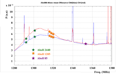
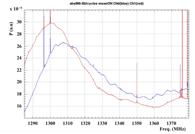
Figure 12: left: mean of BAORadio ON spectra without RFI filtering for both polarizations (polar. 0: blue and polar. 1: red), corresponding to a time slice of 86.4 s from Abell85 observation; the stars mark the frequencies where the $\mathrm{H_{I}}$ signal is expected (see Table 1). right: mean of BAORadio ON-source spectra over the full data set for Abell85 observations (i.e. 652 cycles) processed with median filter in time

With BAORadio, it is possible for instance to produce time-frequency maps with ($0.6$ sec, $30.5$ kHz) resolution by taking the mean of 5120 BRPaquets. Using the same data of Fig. 12 (top), two such maps are shown in Fig. 3.

We have identified several RFIs: three strong ones at 1290 MHz, 1340 MHz and 1361 MHz, and four weaker at 1295 MHz, 1315 MHz, 1335 MHz and 1350 MHz, all with cadences of either 5 sec or 10 sec. These signals might be emitted by the civil air traffic control radars in the Parisian region entering by low level backward lobes created by the East-West geometry of the large mirrors. We find as well electronic RFI at 1300 MHz and 1350 MHz which are permanent, so in the time-frequency image appear as a continuous thin line of thickness given by the lowest possible $\Delta\nu$ of 30 kHz. Such electronic pollutions have been investigated afterwards on test bench and it appears that the most likely source was certainly our local oscillator.

To tackle the above intermittent RFI, a median filter algorithm has been applied on the 8192 frequency components along the time axis with a depth of 5120 digitization frame, corresponding to  0.64 second.

The result obtained is presented in Fig. 12 (bottom) with all the statistics available (i.e. not only the few seconds of Fig. 12 (top), showing the gain in terms of removing spikes and decreasing the fluctuations. Our RFI cleaning filter removes most of the intermittent RFI signals listed above. At 1300 MHz and 1350 MHz, the permanent narrow RFIs generated by the electronic system itself, obviously remain after median filtering over time. We also see a residual RFI at about 1296.4 MHz which might be a tail of the radar at 1295 MHz.

A.2 BAORadio data quality and system stability

We have collected data from the three Abell clusters observations from March to December 2011, using the BAORadio electronic and acquisition system. Figure 14 shows the average power as function of the integration time in a 1 MHz wide band around the central frequency $\nu_{obs}$ for each cluster, computed from $\langle\mathrm{(On-Off)/Off}_{filt}\rangle$ spectra, in black for the complete data set, and in red, for the selected cycles.

We have used few selection criteria to reject low quality or noisy data. The system was unstable during september 2011, although we have not identified clearly the origin of the instability. The corresponding data sets have been dismissed, as well as observations affected by the Sun transit. Finally, we have applied loose cuts on $\langle\mathrm{(On-Off)/Off}_{filt}\rangle$ distribution to reject abnormal observations. The selected data sets are shown in red in Fig. 14 as a function of the cycle number for the three clusters. This corresponds to an overall selection efficiency greater than 99%. We remind however that the BAORadio data acquisition useful time fraction ON-sky was 25% due to network data flow limitation (see Sec.2.2). In addition, Abell2440 observations were not used for $\mathrm{H_{I}}$ emission line search due to limited integration time and the presence of strong RFI in the frequency range of interest.

A.3 Calibration cross-check with NGC4383

To confirm that the 3C161  calibration method was correct (Sec. 3.3), we have observed the NGC4383  source which has both a continuum and a $\mathrm{H_{I}}$ line of $\sim$1-MHz width in the range $[1412,1413]$ MHz. Figure 14 displays the mean over 4 cycles of $\langle\mathrm{(On-Off)/Off}_{filt}\rangle$ spectrum in the range $[1400,1425]$ MHz with the BAORadio system. The $\mathrm{H_{I}}$ line is clearly visible well above the continuum and the stochastic noise. Using the calibration coefficient determined with the 3C161  radiometric source, one finds a $\mathrm{H_{I}}$ line strength of $41.1\pm 1.4(stat)\pm 1.1(syst)$ Jy.km/s which is quite in agreement with the value $48.4\pm 5.1$ Jy.km/s reported in reference (Chung et al.,, 2009, 2010). Notice also that this source is not supposed to be stable and strong enough for calibration purpose.

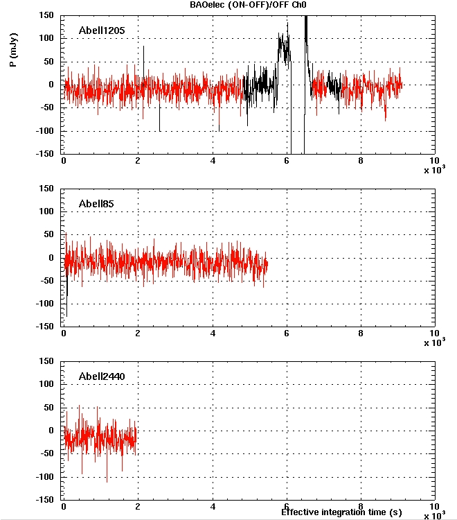
Figure 13: Time evolution of BAORadio $\langle\mathrm{(ON-OFF)/OFF}_{filt}\rangle$ integrated over 1 MHz centered on 1321 MHz for Abell1205 (top), 1346 MHz for Abell85 (middle) and 1302 MHz for Abell2440 (bottom). The effective cycle time sampling of about 8.4 s per data point is used. The whole data set is plotted in black, the data selected for analysis are in red (see text)

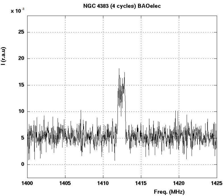
Figure 14: The mean value of $\langle\mathrm{(On-Off)/Off}_{filt}\rangle$ in relative arbitrary units over the two polarizations and over 4 ON-OFF cycles with the BAORadio system on NGC4383 source. We see the $\mathrm{H_{I}}$ line well above the continuum

Appendix B NRT standard auto-correlator data analysis

In this section we describe the analysis done on the data sets from the same observations, acquired in parallel with the NRT standard auto-correlator (ACRT), in order to compare its performance to the BAORadio system, especially in terms of sensitivity. For this analysis we have used the standard NRT software tools as well as a specific data reduction pipeline similar to the BAORadio one.

B.1 ACRT description

The NRT standard auto-correlator consists roughly of a mid-frequency amplifier and a Control Auto de Gain (CAG) that scales the input to 2 V, after which it is split into two parallel chains:

• The filter chain measures the total power received in the whole bandwidth vs. time which is digitized with a 12-bit ADC and a SEFRAM (rapid digitization at 4 to 500 Hz).

• The digital correlator chain (ACRT) measures the total power received and the signal vs. time and computes the auto-correlation of the signal. The output at hardware level is the total power received and the power spectrum normalized to the total power received, both digitized with a 3-bits 9-level ADC.

The digital auto-correlator has a total bandwidth that can be set from 200 kHz to 50 MHz. The 8192 frequency channels can be split into 2 to 8 banks. In our case we have set up a 25-MHz bandwidth and 4 banks which correspond to 2 linear polarizations and 2 circular polarizations (not analyzed). This gives 2048 channels per bank and a frequency resolution of 12.2 kHz. The NRT acquisition chains are 100% efficient ON-sky, and the minimum integration time is 1-sec. This has to be compared to BAORadio system which had 25% on sky efficiency, but a time resolution of 16.7 ms. The NRT provides standard tools (NAPS) to pre-process and calibrate raw observations.

B.2 ACRT data quality and system stability

The whole ACRT data set extend by one month (i.e. January 2012) the data set acquired with the BAORadio system. Similar selection criteria as the ones listed in Section A.2 were applied, as well as an additional cut on the first 10-sec of each cycle as the signal is affected by the stretching of the 150 m long cable carrying the analog signal out of the chariot. This happens when the chariot repositions itself between the end of the ON phase and the beginning of the OFF phase. A striking illustration of the effect of the cable stretching can be seen on Fig. 15 where the difference of the total power collected in ON and OFF phases for the polarization p0 is presented as function of time. Notice the same trend is also observed on p1 (not shown). We observe a ”pan flute” pattern due to the tail after the DAB pulse during the OFF phase which can last for about 10 sec maximum. This cable stretching is responsible for 25% loss of 1-sec integrations for ACRT and is the main source of inefficiency. The BAORadio system is not affected by cable stretching as the digitization is done in the chariot as close as possible to the first preamplifier and filters chain.

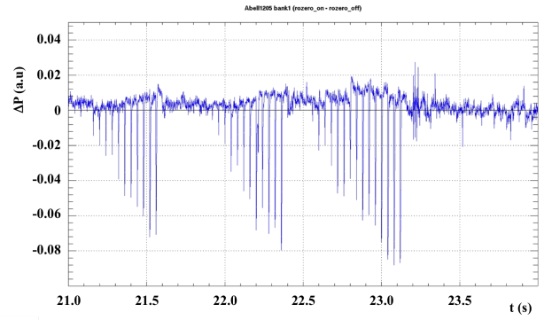
Figure 15: Difference of total power received in ON and OFF phases vs. time for polarization p0 to illustrate the effect of cable stretching in the signal. The zero value is marked with a black line

Similarly to Figure 14 for BAORadio, we show in Figure 17 the time evolution of the mean values $\langle\mathrm{(On-Off)/Off}_{filt}\rangle$ over 1 MHz centered on the central frequency in ACRT observation band for each cluster (see Table 1). The whole data set is presented in black and the selected data for analysis (including RFI-cleaning) in red.

Table 5 summarizes the observations kept after the quality cuts for both BAORadio and ACRT. It is clear that ACRT system currently suffers from analog signal propagation, making it less efficient than BAORadio despite its intrinsic ON-sky efficiency of 100%.

Table 5: Efficiency and integration time ON-sky of ACRT and BAORadio in terms of fraction of useful cycles used after quality cuts and RFI-cleaning procedure. We remind that the efficiency ON-sky is 100% for ACRT and 25% for BAORadio

Cluster	System	Total cycles	Useful cycles	Efficiency	Integration ON-sky
Abell1205	ACRT	1374	741	53.9 %	29 640 s
	BAORadio	840	837	99.6 %	6 277 s
Abell2440	ACRT	320	141	44.1 %	5 640 s
	BAORadio	230	230	100.0 %	1 725 s
Abell85	ACRT	737	287	38.9 %	11 480 s
	BAORadio	652	651	99.8 %	4 882 s

B.3 ACRT data analysis

The ACRT system outputs for each polarization the total power received and the autocorrelation of the signal normalized to this power. For the analysis we have taken as ”raw spectra” the product of the normalized autocorrelation signal and the total power received for each 1-sec integration. We have then applied a similar analysis method as for BAORadio: selection of data (quality cuts and RFI-cleaning, described below), obtention of $\langle\mathrm{(On-Off)/Off}_{filt}\rangle$ spectrum and time series analysis of the mean signal integrated on 1 MHz band around the cluster observation frequency to obtain the radiometric curve.

We have cleaned the data from RFI using two algorithms. The first one consists of eliminating the integrations that significantly differ in spectral power from the mean of a given phase (ON or OFF), which could be the case of spectra with extra noise or affected by RFI. This is done computing along the frequency axis the standard deviation between the 1-sec integration spectra and a mean frequency spectrum over the whole phase considered, and rejecting those integrations with a standard deviation above a threshold. This algorithm is inspired on the Integration Limit RMS algorithm, nicknamed ”ILR” and implemented on the NRT standard software analysis NAPS (Renaud,, 2007). The second RFI-cleaning algorithm searches for intermittent radar signals appearing as peaks in the time evolution of the total power received. As this power is digitized with a small dynamic range, we enhance the peaks considering instead the ”total radar power”, defined as the sum of 2-MHz bands centered on the known radar signals seen in Fig. 3.

The combination of the two RFI-cleaning algorithms rejects 27% of the data for Abell1205, 47% for Abell85 and 41% for Abell2440.

B.4 ACRT calibration

During a cycle, diode pulses (DAB) are injected in the NRT horn at the beginning of an acquisition phase (ON and OFF). In general this kind of known injection power is used as default calibration thanks to the conversion relation determined with dedicated observations of well-known calibrator sources during NRT special runs (Fouque et al.,, 1990). But during our cluster observations this routine procedure has shown surprisingly that the system is much more stable than the DAB itself.

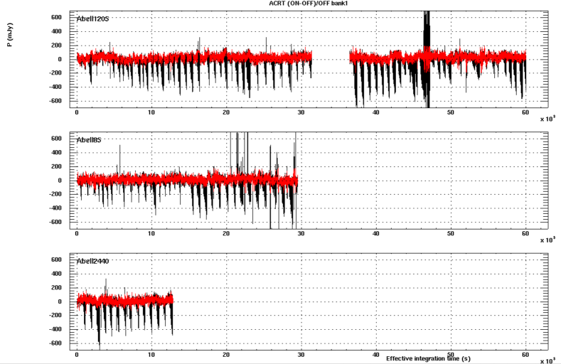
Figure 16: Time evolution of ACRT $\langle\mathrm{(On-Off)/Off}_{filt}\rangle$ integrated signal in 1 MHz band around the observation frequency of each cluster: in black the complete data set of observations, in red the subset of observations kept after quality cuts

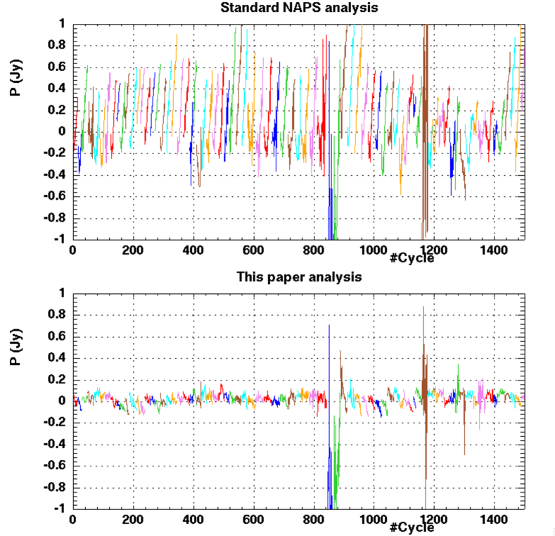
Figure 17: ACRT mean $\langle\mathrm{(On-Off)/Off}_{filt}\rangle$ signal integrated in the band $[1320.3,1321.3]$ MHz versus the cycle number for polarization p0, obtained from the standard NAPS analysis (top) and from the analysis presented in this paper (Sec.3.3) (bottom)

This is illustrated in Figure 17, where we show the mean signal integrated in 1-MHz band around the observation frequency for Abell1205 observations plotted versus the cycle number. Different observation dates are distinguished by different colors. On the top panel we have used as input the DAB-calibrated spectra obtained with standard NAPS tools. On the bottom panel we use as input the ”raw spectra” and the calibration is done with the radio source 3C161  (from dedicated ”drift scan” observations, in a similar way to that explained in Section 3.3.1). No data selection or RFI-cleaning algorithm is used in any case.

We see that the NAPS-calculated mean signal systematically increases from the beginning to the end of an observation, the maximum variation lies between approximatively 200 mJy and 1.2 Jy. This bias is not seen on the bottom panel, and it is clearly introduced by the DAB pulses. It is the main reason why we have done calibration using 3C161  observations and we have build a special pipeline to analyze the ACRT data. This is the same conclusion as for the BAORadio pipeline (see Sec. 3.3).

Nevertheless, it is worth saying that the NRT pipeline and analysis tools and methods are optimized to search for known lines (frequency and width), and it is not adequate for the blind search we do in this study, as we have shown.

References

- Ansari et al., (2012a) Ansari, R., Campagne, J.E., Colom, P., Le Goff, J.M., Magneville, C. et al., 21 cm observation of large-scale structures at z ~ 1. Instrument sensitivity and foreground subtraction, A&A, 540, A129, , 1108.1474.
- Ansari et al., (2012b) Ansari, R., Campagne, J.E., Colom, P., Magneville, C., Martin, J.M. et al., BAORadio: A digital pipeline for radio interferometry and 21 cm mapping of large scale structures, Comptes Rendus Physique, 13, (2012b), 46, , 1209.3266.
- Ansari et al., (2008) Ansari, R., Le Goff, J.., Magneville, C., Moniez, M., Palanque-Delabrouille, N. et al., Reconstruction of HI power spectra with radio-interferometers to study dark energy, ArXiv e-prints, 0807.3614.
- Auld et al., (2006) Auld, R., Minchin, R.F., Davies, J.I., Catinella, B., van Driel, W. et al., The Arecibo Galaxy Environment Survey: precursor observations of the NGC 628 group, MNRAS, 371, (2006), 1617, , astro-ph/0607452.
- Baars et al., (1977) Baars, J.W.M., Genzel, R., Pauliny-Toth, I.I.K. and Witzel, A., The absolute spectrum of CAS A - an accurate flux density scale and a set of secondary calibrators, A&A, 61, (1977), 99.
- Bandura, (2011) Bandura, K., Pathfinder for a Neutral Hydrogen Dark Energy Survey, Ph.D. thesis, Carnegie Mellon University (2011).
- Bravo-Alfaro et al., (2009) Bravo-Alfaro, H., Caretta, C.A., Lobo, C., Durret, F. and Scott, T., Galaxy evolution in Abell 85. I. Cluster substructure and environmental effects on the blue galaxy population, A&A, 495, (2009), 379, , 0811.2686.
- Bravo-Alfaro et al., (2008) Bravo-Alfaro, H., van Gorkom, J.H. and Caretta, C., Environmental effects in the cluster Abell 85 (z=0.055): An HI Imaging Survey and a Dynamical Study, in Y.V. Baryshev, I.N. Taganov and P. Teerikorpi (editors) Problems of Practical Cosmology, Volume 1, pages 102–105 (2008).
- Charlet et al., (2011) Charlet, D., Abbon, P., Ansari, R., Beigbeder, C., Breton, D. et al., The BAO Radio Acquisition System, IEEE Transactions on Nuclear Science, 58, (2011), 1833, .
- Chen, (2012) Chen, X., The Tianlai Project: a 21CM Cosmology Experiment, International Journal of Modern Physics Conference Series, 12, (2012), 256, , 1212.6278.
- Chung et al., (2009) Chung, A., van Gorkom, J.H., Kenney, J.D.P., Crowl, H. and Vollmer, B., VLA Imaging of Virgo Spirals in Atomic Gas (VIVA). I. The Atlas and the H I Properties, AJ, 138, (2009), 1741, .
- Chung et al., (2010) Chung, A., van Gorkom, J.H., Kenney, J.D.P., Crowl, H. and Vollmer, B., Erratum: VLA Imaging of Virgo Spirals in Atomic Gas (VIVA). I. The Atlas and The H I Properties (2009, AJ, 138, 1741), AJ, 139, 2716, , 0909.0781.
- Cortese et al., (2008) Cortese, L., Minchin, R.F., Auld, R.R., Davies, J.I., Catinella, B. et al., The Arecibo Galaxy Environment Survey - II. A HI view of the Abell cluster 1367 and its outskirts, MNRAS, 383, (2008), 1519, , 0711.0684.
- Durret et al., (1998a) Durret, F., Felenbok, P., Lobo, C. and Slezak, E., A catalogue of velocities in the cluster of galaxies Abell 85, A&AS, 129, (1998a), 281, , astro-ph/9709298.
- Durret et al., (1998b) Durret, F., Forman, W., Gerbal, D., Jones, C. and Vikhlinin, A., The rich cluster of galaxies ABCG 85. III. Analyzing the ABCG 85/87/89 complex, A&A, 335, (1998b), 41, astro-ph/9802183.
- Fouque et al., (1990) Fouque, P., Durand, N., Bottinelli, L., Gouguenheim, L. and Paturel, G., An HI survey of late-type galaxies in the Southern Hemisphere. I - The SGC sample, A&AS, 86, (1990), 473.
- Granet et al., (1999) Granet, C., James, G.L. and Pezzani, J., The full-size dual-reflector feed system for the Nançay radio telescope., Journal of Electrical and Electronics Engineering Australia, 19, (1999), 111.
- Haynes et al., (2011) Haynes, M.P., Giovanelli, R., Martin, A.M., Hess, K.M., Saintonge, A. et al., The Arecibo Legacy Fast ALFA Survey: The .40 H I Source Catalog, Its Characteristics and Their Impact on the Derivation of the H I Mass Function, AJ, 142, 170, , 1109.0027.
- Kalberla et al., (2005) Kalberla, P.M.W., Burton, W.B., Hartmann, D., Arnal, E.M., Bajaja, E. et al., The Leiden/Argentine/Bonn (LAB) Survey of Galactic HI. Final data release of the combined LDS and IAR surveys with improved stray-radiation corrections, A&A, 440, (2005), 775, , astro-ph/0504140.
- Lima Neto et al., (2001) Lima Neto, G.B., Pislar, V. and Bagchi, J., BeppoSAX observation of the rich cluster of galaxies Abell 85, A&A, 368, (2001), 440, , astro-ph/0101060.
- Meyer et al., (2004) Meyer, M.J., Zwaan, M.A., Webster, R.L., Staveley-Smith, L., Ryan-Weber, E. et al., The HIPASS catalogue - I. Data presentation, MNRAS, 350, (2004), 1195, , astro-ph/0406384.
- Monnier Ragaigne et al., (2003) Monnier Ragaigne, D., van Driel, W., Schneider, S.E., Balkowski, C. and Jarrett, T.H., A search for Low Surface Brightness galaxies in the near-infrared. III. Nançay H I line observations, A&A, 408, (2003), 465, , astro-ph/0305319.
- Ott et al., (1994) Ott, M., Witzel, A., Quirrenbach, A., Krichbaum, T.P., Standke, K.J. et al., An updated list of radio flux density calibrators, A&A, 284, (1994), 331.
- Parsons et al., (2009) Parsons, A., Werthimer, D., Backer, D., Bastian, T., Bower, G. et al., Digital Instrumentation for the Radio Astronomy Community, in astro2010: The Astronomy and Astrophysics Decadal Survey, volume 2010 of Astronomy, page 21 (2009), 0904.1181.
- Peterson et al., (2009) Peterson, J.B., Aleksan, R., Ansari, R., Bandura, K., Bond, D. et al., 21-cm Intensity Mapping, in astro2010: The Astronomy and Astrophysics Decadal Survey, volume 2010 of Astronomy, page 234 (2009), 0902.3091.
- Pustilnik et al., (2002) Pustilnik, S.A., Martin, J.M., Huchtmeier, W.K., Brosch, N., Lipovetsky, V.A. et al., Studies of galaxies in voids. I. H I observations of Blue Compact Galaxies, A&A, 389, (2002), 405, , astro-ph/0205195.
- Renaud, (2007) Renaud, P., NAPS User Guide (French), Technical report, USN - Unité Scientifique de la Station de Nançay (2007).
- Rostagni, (2014) Rostagni, F., Classification morphologique d’un échantillon optique d?amas de galaxies, Ph.D. thesis, Université de Nice - SOPHIA ANTIPOLIS (2014).
- Slezak et al., (1998) Slezak, E., Durret, F., Guibert, J. and Lobo, C., A photometric catalogue of galaxies in the cluster Abell 85, A&AS, 128, (1998), 67, , astro-ph/9710103.
- Szymczak, M. and Gerard, E., (2004) Szymczak, M. and Gerard, E., Polarimetric observations of oh masers in proto-planetary nebulae, Astron.Astrophys., 423, (2004), 209, , astro-ph/0405316.
- Tanaka et al., (2010) Tanaka, N., Furuzawa, A., Miyoshi, S.J., Tamura, T. and Takata, T., Suzaku Observations of the Merging Cluster Abell 85: Temperature Map and Impact Direction, PASJ, 62, (2010), 743, , 1006.4328.
- Taylor et al., (2012) Taylor, R., Davies, J.I., Auld, R. and Minchin, R.F., The Arecibo Galaxy Environment Survey - V. The Virgo cluster (I), MNRAS, 423, (2012), 787, , 1203.3094.
- Taylor et al., (2013) Taylor, R., Davies, J.I., Auld, R., Minchin, R.F. and Smith, R., The Arecibo Galaxy Environment Survey - VI. The Virgo cluster (II), MNRAS, 428, (2013), 459, , 1209.4338.
- van Driel et al., (2001) van Driel, W., Gao, Y. and Monnier-Ragaigne, D., H I line observations of luminous infrared galaxy mergers, A&A, 368, (2001), 64, , astro-ph/0101003.
- van Driel et al., (1997) van Driel, W., Pezzani, J. and Gerard, E., Renovating the Nançay radio telescope: the FORT project, page 229.
- van Driel et al., (2009) van Driel, W., Schneider, S., Lehnert, M., Blyth, S., Bouchard, A. et al., NIBLES: an HI census of SDSS galaxies in the Local Volume, in Panoramic Radio Astronomy: Wide-field 1-2 GHz Research on Galaxy Evolution, page 8 (2009).
- Verheijen et al., (2007) Verheijen, M., van Gorkom, J.H., Szomoru, A., Dwarakanath, K.S., Poggianti, B.M. et al., WSRT Ultradeep Neutral Hydrogen Imaging of Galaxy Clusters at z ~ 0.2: A Pilot Survey of Abell 963 and Abell 2192, ApJ, 668, (2007), L9, , 0708.3853.