Massive stars in the W33 giant molecular complex.

Abstract

Rich in HII regions, giant molecular clouds are natural laboratories to study massive stars and sequential star formation. The Galactic star forming complex W33 is located at $l=\sim 12\fdg 8$ and at a distance of 2.4 kpc, has a size of $\approx 10$ pc and a total mass of $\approx(0.8-−8.0)\times 10^{5}$ M_⊙. The integrated radio and IR luminosity of W33 - when combined with the direct detection of methanol masers, the protostellar object W33A, and protocluster embedded within the radio source W33 main - mark the region out as a site of vigorous ongoing star formation. In order to assess the long term star formation history, we performed an infrared spectroscopic search for massive stars, detecting for the first time fourteen early-type stars, including one WN6 star and four O4-7 stars. The distribution of spectral types suggests that this population formed during the last $\sim 2-4$ Myr, while the absence of red supergiants precludes extensive star formation at ages $6-30$ Myr. This activity appears distributed throughout the region and does not appear to have yielded the dense stellar clusters that characterize other star forming complexes such as Carina and G305. Instead, we anticipate that W33 will eventually evolve into a loose stellar aggregate, with Cyg OB2 serving as a useful, albeit richer and more massive, comparator. Given recent distance estimates, and despite a remarkably similar stellar population, the rich cluster Cl 1813$-$178 located on the north-west edge of W33 does not appear to be physically associated with W33.

1. Introduction

Massive stars enrich the galactic interstellar medium via the feedback of radiative and mechanical energy, the deposition of chemically processed gas via their strong winds and, latterly, solid state material during the post main-sequence (MS) phase. Because of their luminosities, individual massive stars can be detected and resolved in external galaxies, providing direct measures of distances and spatially resolved metallicity gradients (e.g., Kudritzki et al. 2014). At and beyond the end of their lives they power a wide variety of highly energetic transient phenomena - firstly during their deaths in supernovae or gamma-ray bursts and subsequently by accretion onto their stellar corpses in X-ray binaries (e.g., Güdel & Nazé 2009; Eldridge et al. 2013).

Considerable uncertainty remains regarding the mechanism(s) of formation of massive stars, although it is strongly suspected that this process is hierarchical: massive stars are found in apparently isolated young massive stellar clusters (e.g., the Arches and Quintuplet clusters; Figer et al. 2002), in loose associations (e.g., Cyg OB2; Wright et al. 2014; Negueruela et al. 2008, and refs. therein), and in large molecular complexes (e.g., 30 Doradus and G305; Walborn & Blades 1997; Clark & Porter 2004).

Massive stars are very often part of binary systems ( typically, a fraction of 91% of OB stars is found to have companions, Sana et al. 2014). A population of apparently isolated massive stars also exists, although it is not clear whether these have genuinely formed in isolation (e.g., Bestenlehner et al. 2011) or, instead, were lost from a natal aggregate due to dynamical or supernova driven ejection (runaway stars, Oh et al. 2014; Povich et al. 2008).

Because of the high and variable interstellar extinction and uncertain distances of stars within the Galactic Disk, it has long been suspected that our census of massive star forming regions is incomplete. Fortunately, the plethora of modern infrared and radio surveys - e.g., MAGPIS, GLIMPSE, WISE, MSX, 2MASS, UKIDSS, and VVV , - allow us to identify both the natal giant molecular clouds (GMCs) and the stars that form within them. Subsequent analysis of the physical properties of GMCs and associated stellar population(s) - in terms of the mass function of pre-stellar clumps/cores (proto-stars), and already formed massive stars, and their temporal and spatial distributions - enable constraints to be placed on the mode of star formation that occurred in the region in question (e.g., Messineo et al. 2014a).

One such massive star forming region is the W33 complex, located in the Galactic plane at longitude $l=\sim 12\fdg 8$; a parallactic distance of $2.40^{+0.17}_{-0.15}$ kpc was determined from observations of water masers, which suggests a location in the Scutum spiral arm (Immer et al. 2013). Subtending 15^′ ($\sim 10$ pc), it comprises a number of distinct molecular and/or dusty condensations (see Immer et al. 2014 for a census), with an integrated IR luminosity of $\sim 8\times 10^{5}$ L_⊙ and a total mass of $\sim(0.8-8)\times 10^{5}M_{\odot}$ (Immer et al. 2013). Radio observations of one component - W33 Main - revealed the presence of an obscured (proto-)cluster apparently comprising a number of stars with spectral types ranging from O7.5 to B1.5 (Haschick & Ho 1983). The presence of ongoing massive star formation is also signposted by the presence of OH, H₂O, and CH₃OH masers (Immer et al. 2013), and the direct identification of a bipolar outflow and massive dusty torus associated with the young stellar object W33A (Davies et al. 2010).

Independently of these studies, Messineo et al. (2008, 2011) serendipitously identified a hitherto overlooked young massive cluster - Cl 1813$-$178 - in the vicinity of W33. Analysis of the post-MS content of the cluster suggested a mass $\gtrsim 10^{4}M_{\odot}$, making it amongst the most massive aggregates in the Galaxy (Clark et al. 2013). Given the unusual mix of spectral types present, Messineo et al. (2011) quoted 4-4.5 Myr, but highlighted that several cluster members had low luminosities for that age; stellar luminosities would appear to demonstrate some degree of non-coevality. Intriguingly, Cl 1813$-$178 is found in the vicinity of the pulsar wind nebula HESS J1813$-$178 (Helfand et al. 2007; Messineo et al. 2008). With a spin-down measurement of 44.7ms and a spin-down luminosity of $\dot{E}\sim 5.6\times 10^{37}$erg s^-1, PSR J1813$-$1749 is one of the youngest and most energetic pulsars in the Galaxy (Halpern et al. 2012). While the energetic young pulsar potentially lies beyond both regions ($>4.8$ kpc, Halpern et al. 2012); evidently, this line-of-sight samples numerous regions of massive star formation.

Here, we present a near-infrared spectroscopic survey of bright stars in selected regions of W33 (cl1, cl2, and Mercer1, Messineo et al. 2011), and in the nearby GLIMPSE bubble N10 (e.g., Churchwell et al. 2006). We aim to determining the massive stellar content of W33, its star formation history, and, hence, relation to the nearby cluster Cl 1813$-$178 and pulsar PSR J1813$-$1749. In Sect. 2, we present the spectroscopic observations, and in Sect. 3, the available infrared photometry. In Sect. 2, we present the spectroscopic observations, and in Sect. 3, the available infrared photometry. In Sect. 4, we describe the spectral features and stellar properties. In Sects. 6, 7, and 8, we briefly describe the spatial and temporal distributions of the detected stars, before summarising our findings in Sect. 9.

2. Targets and spectroscopic observations

Spectroscopic targets with 2MASS K_s from 6 mag to 11 mag and $H-$K_s$>0.5$ mag were selected from the regions listed in Messineo et al. (2011) that exhibited over-densities of bright stars or nebulae in 2MASS and GLIMPSE images. The Mercer1 region, to the west of the radio source W33 Main, appears as a sparse aggregate of bright stars with a pronounced arc of IR and radio emission to the south that is suggestive of a wind blown structure (Fig.1, top panel). The cl1 region, immediately to the east of the embedded proto-cluster in W33 Main, contains an isolated bright star surrounded by an arc of emission at IR and radio wavelengths (Fig. 1, middle panel). The cl2 region, coincident with W33 B1 (e.g., Immer et al. 2014), contains a small cluster of stars associated with diffuse IR and radio emission (Fig. 1, bottom panel). These targets were supplemented with a few isolated bright targets selected on the basis of their GLIMPSE colors - e.g., indicative of free-free emitters (e.g., Hadfield et al. 2007; Messineo et al. 2012)) - such as star #1 and the candidate luminous blue variable (LBV) #15 from Cl 1813$-$178. Additionally, we observed some stars to the north of W33, in the cluster BDS2003-115 embedded in the GLIMPSE mid-IR bubble N10 (Fig. 2).

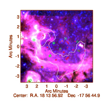
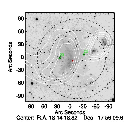
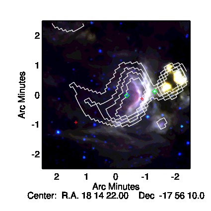
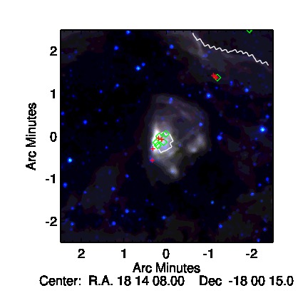
Figure 1.— Images of the stellar clusters Mercer1 ( top row), cl1 ( middle row), and cl2 ( bottom row) in W33 (Messineo et al. 2011). Left side: detected stars are displayed on a UKIDSS $K$-band image (for cl2 the $J$ image is used). Diamonds and crosses indicate the positions of detected early-types and late-types, respectively. Contours of the 90 cm radio-continuum emission from 100 up to 400 mJy beam^-1 (with a step of 100 mJy beam^-1) are shown in white. The two dashed circles mark the regions used for the CMDs in Fig. 8. By assuming a distance of 2.4 kpc, one arcminute corresponds to 0.70 pc. Right side: contours of the 90 cm radio-continuum emission superimposed on a GLIMPSE composite image (3.6 $\mu$m in blue, 5.8 $\mu$m in green, and 8.0 $\mu$m in red).

Data were acquired with the Spectrograph for INtegral Field Observations in the Near Infrared (SINFONI, Eisenhauer et al. 2003) on the Yepun Very Large Telescope, under the ESO programs 087.D-0265(A) and 089.D-0790(A). The $K$-grating was used along with the $0\hbox to0.0pt{.\hss}^{\prime\prime}25$ pix^-1 scale to yield a resolving power of $\sim 4500$. Integration times per exposure ranged from 30 s to 300 s. Typically, each observation consisted of four exposures, two on target and two on sky. Data-cubes were generated with the version 3.9.0 of the ESO SINFONI pipeline (Schreiber et al. 2004; Modigliani et al. 2007), using flat-fields, bad-pixel masks, distortion maps, and arcs. From each cube, stellar traces with signal-to-noise ratio larger than 30-40 were analyzed. Corrections for instrumental and atmospheric responses were accomplished with standard stars of B-types; stellar Br_γ  and He I lines at 2.112 $\mu$m were removed from the standard spectra with a linear interpolation. A sky subtraction was performed to eliminate possible nebular lines and residuals from OH subtraction. A total of 86 cubes were observed and 94 stars were extracted.

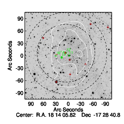
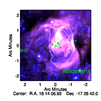
Figure 2.— Images of the bubble N10. Left side: Detected stars are displayed on a UKIDSS $K$-band image. Diamonds and crosses indicate the positions of detected early-types and late-types, respectively. The white contours show the 90 cm radio-continuum emission of the bubble N10 from MAGPIS at 100, 200, and 300 mJy beam^-1. By assuming a distance of 4.29 kpc, one arcminute corresponds to 1.25 pc. Right side: The 90 cm contours are superimposed on a GLIMPSE composite image (3.6 $\mu$m in blue, 5.8 $\mu$m in green, and 8.0 $\mu$m in red).

3. Available photometric data

We searched for counterparts of the spectroscopically observed stars in the 2MASS Catalog of Point Sources (Skrutskie et al. 2006), in the UKIDSS catalog (UKIDSS, Lucas et al. 2008), and in the DENIS catalog (DENIS, DENIS Consortium 2005) by taking the closest match within 1^′′. Mid-infrared data were retrieved from the MSX (MSX, Egan et al. 2003) with a search radius of 5^′′, from the GLIMPSE (GLIMPSE, Churchwell et al. 2009) and The WISE (WISE, Wright et al. 2010) catalogues with a search radius of 2^′′.

For 21% of the sources, $R$-band counterparts with magnitudes from 12.38 mag to 19.80 mag were found in the The Naval Observatory Merged Astrometric Dataset (NOMAD) (Zacharias et al. 2004).

Photometric measurements are listed in the appendix. For the observed targets, there is no additional information from the SIMBAD database.

3.1. UKIDSS photometry

For stars fainter than K_s$\sim 10.5$ mag, we used UKIDSS photometry (Lucas et al. 2008). $JHK$ magnitudes are available from the UKIDSS data release number 6 (DR6) (Lucas et al. 2008); however, for four fields (Mercer1, cl1, cl2, N10) we generated photometric catalogs of point sources with the psf-fitting algorithm DAOPHOT (Stetson 1987) and the leavestack frames provided by UKIDSS (Lucas et al. 2008). A detection threshold of 4 $\sigma$ was used. From overlapping fields, independently calibrated with 2MASS datapoints, an absolute photometric error of 0.05 mag was estimated. Comparison of the UKIDSS pipeline and the psf-fitting catalogs in the Mercer1 field yielded an absolute uncertainty of 0.07 mag. The resultant magnitudes are given in the appendix.

4. Analysis

4.1. Spectral classification

We detected a total of 23 new early-types, which comprise one Wolf-Rayet, 13 stars of spectral type O or B, and nine stars with indeterminate, but early, spectral types (OBAF), and 70 late-type stars (see Tables 1, 2, and 3).

Table 1 Summary of Observations of Early-type Stars.

ID	Ra[J2000]	Dec[J2000]	Spec.	Period	Date-Obs
	[hh mm ss]	[deg mm ss]			yyyy-mm-dd
M15a	18 13 20.99	-17 49 46.9	cLBV	P89	2012-06-21
1	18 13 34.81	$-$18 05 41.5	WN6	P89	2012-06-21
2	18 13 47.53	$-$17 57 10.7	OBAF	P89	2012-06-27
3	18 13 48.07	$-$17 56 15.6	B0-5	P87	2011-08-19
4	18 13 53.10	$-$17 55 57.3	B0-5	P87	2011-05-29
5	18 13 55.36	$-$17 57 00.7	OBAF	P87	2011-05-29
6	18 13 58.19	$-$17 56 23.9	B0-5	P87	2011-05-29
7	18 13 58.20	$-$17 56 25.4	O4-6	P87	2011-05-29
8	18 13 59.69	$-$17 57 41.2	O4-6	P87	2011-08-19
9	18 13 59.83	$-$17 57 44.4	OBAF	P87	2011-08-20
10	18 14 03.00	$-$17 58 52.3	B0-5	P87	2011-08-20
11	18 14 05.69	$-$17 28 40.3	O4-6	P87	2011-06-24
12	18 14 06.12	$-$17 28 33.2	OBAF	P87	2011-06-24
13	18 14 06.63	$-$17 56 06.3	B0-5	P87	2011-08-26
14	18 14 06.89	$-$17 28 43.2	OBe	P89	2012-09-15
15	18 14 06.93	$-$17 28 45.5	OBAF	P89	2012-09-15
16	18 14 07.89	$-$17 28 40.9	OBAF	P89	2012-09-15
17	18 14 08.09	$-$18 00 11.6	B0-5	P89	2012-06-26
18	18 14 08.30	$-$18 00 23.3	B0-5	P87	2011-05-29
19	18 14 08.74	$-$18 00 15.2	OBAF	P89	2012-06-26
20	18 14 08.89	$-$18 00 27.8	OBAF	P89	2012-09-15
21	18 14 09.03	$-$18 00 23.8	OBAF	P89	2012-09-15
22	18 14 16.52	$-$17 56 03.2	Oe	P87	2011-05-29
23	18 14 20.48	$-$17 56 11.2	O6-7	P87	2011-05-29

• Star $[$MFD2011$]$ 15 was discovered by Messineo et al. (2011).

4.1.1 Early-type stars

Figure 3.— SINFONI $K-band$ spectra of newly detected O-type stars. Panel (a) displays massive O-type stars, panel (b) B-type stars, and panel (c) spectra (mostly marginal detections) with a detection of a Br_γ line.

Figure 4.— Upper panel: SINFONI $K$-band spectrum of a newly detected WN6 star. Lower panel: SINFONI $K$-band spectrum of the candidate LBV [MFD2011] 15.

The spectra of the newly-discovered early-type stars are characterized by hydrogen and helium lines, as well as transitions of heavier elements, such as C, N, O, and Fe. Their spectral classification was accomplished by comparison to the near-infrared atlases of Hanson et al. (1996), Hanson et al. (2005), and Figer et al. (1997).

Star #1 is a newly discovered Wolf-Rayet star; its spectrum is characterized by strong and broad emission lines; He I/ N III centered at 2.1117 $\mu$m, He II/ Br_γ line at 2.1636 $\mu$m, and He II at 2.1891 $\mu$m. The equivalent width ratios between the 2.1891 $\mu$m line and the two lines at 2.1636 $\mu$m and 2.112 $\mu$m were estimated to be $1.8\pm 0.3$ and $4.3\pm 0.7$ respectively, by using multiple gaussian fits (Figer et al. 1997). This spectrum resembles that of WR134, a WN6b star (Figer et al. 1997); the suffix b indicates broad emission lines (e.g., Hadfield et al. 2007); derived ratios are almost identical to those calculated for WR134; thereby, star #1 is a WN6b.

The spectra of stars #7, #8, #11, and #23 are characterized by emission in the C IV 2.0705 $\mu$m and 2.0796 $\mu$m and O III/N III at $\approx 2.115$ $\mu$m lines, He I line at 2.059 $\mu$m and He II 2.189 $\mu$m in absorption, and Br_γ mostly in absorption (see Table 2 and Fig. 3). This combination of features is characteristic of stars of mid- to late-O spectral type; unfortunately, for this temperature range the assignment of luminosity classes from K-band spectra alone is somewhat problematic. Nevertheless, in this regard we note the strong morphological resemblance of these objects to the O4-6 I stars within the Arches cluster (Martins et al. 2008). The spectra of stars #8, #11, and #23 display the Si IV emission line at 2.428 $\mu$m. We denote O-type stars with O III/N III and Si IV in emission by Of${}_{K}^{+}$, as described in Messineo et al. (2014a), although we caution that this does not necessarily indicate a super/hyper-giant classification (de Jager 1998). Star #8 has Br_γ filled in, indicating I+ nature. The spectrum of star #23 has the He I line at 2.112 $\mu$m in absorption, and most likely has a later sub-type.

Table 2 List of Lines Detected in Early-type Stars

ID	Center	FWHM	EW∗∗	SN+	VLSR++
	[$\mu$m]	[Å]	[Å]		[km s-1]
M15	2.059024	19 $\pm$ 0	-52.1 $\pm$ 0.4	278	$63\pm 10$
M15	2.166333	26 $\pm$ 0	-33.6 $\pm$ 0.4	355	$44\pm 10$
1	2.045707	$33\pm 0$	12.7 $\pm$ 1.0	6	$..$
1	2.111480	$229\pm 1$	$-$43.1 $\pm$ 5.8	18	$..$
1	2.163296	$199\pm 2$	$-$106.3 $\pm$ 16.3	32	$..$
1	2.188899	$195\pm 1$	$-$186.2 $\pm$ 14.4	68	$..$
2	2.165926	57 $\pm$ 8	6.3 $\pm$ 6.0	7	$..$
3	2.113018	19 $\pm$ 1	1.8 $\pm$ 0.9	10	$..$
3	2.166116	56 $\pm$ 0	6.9 $\pm$ 1.1	27	$..$
4	2.112701	38 $\pm$ 1	1.8 $\pm$ 0.4	12	$..$
4	2.165608	67 $\pm$ 2	3.2 $\pm$ 1.3	10	$..$
$*5$	2.165962	77 $\pm$ 187	2.3 $\pm$ 7.1	4	$..$
6	2.112678	17 $\pm$ 11	2.0 $\pm$ 1.7	4	$..$
6	2.165574	73 $\pm$ 8	4.1 $\pm$ 2.7	6	$..$
7	2.058728	21 $\pm$ 4	0.7 $\pm$ 1.1	5	$..$
7	2.069326	11 $\pm$ 4	-0.2 $\pm$ 0.5	4	$..$
7	2.079126	11 $\pm$ 1	-0.5 $\pm$ 0.5	11	$..$
7	2.115881	32 $\pm$ 0	-1.5 $\pm$ 0.8	8	$..$
7	2.165977	55 $\pm$ 2	3.5 $\pm$ 1.2	13	$..$
7	2.189267	16 $\pm$ 14	1.9 $\pm$ 0.5	11	$..$
$*8$	2.069469	13 $\pm$ 21	-0.4 $\pm$ 0.7	4	$..$
8	2.079379	16 $\pm$ 0	-1.4 $\pm$ 0.6	12	$..$
8	2.115700	46 $\pm$ 0	-4.3 $\pm$ 0.7	15	$..$
8	2.189147	15 $\pm$ 8	0.6 $\pm$ 0.9	4	$..$
8	2.427893	38 $\pm$ 11	-2.1 $\pm$ 2.0	4	$..$
9	2.166162	65 $\pm$ 34	3.4 $\pm$ 3.9	6	$..$
10	2.112934	17 $\pm$ 1	0.5 $\pm$ 1.3	7	$..$
10	2.166113	92 $\pm$ 6	6.9 $\pm$ 1.8	14	$..$
11	2.058704	13 $\pm$ 4	0.4 $\pm$ 2.1	4	$..$
11	2.079061	20 $\pm$ 3	-1.4 $\pm$ 0.8	8	$..$
11	2.115609	38 $\pm$ 3	-2.3 $\pm$ 0.7	12	$..$
11	2.166673	34 $\pm$ 6	2.6 $\pm$ 1.5	11	$..$
11	2.189657	20 $\pm$ 11	1.2 $\pm$ 1.1	6	$..$
$*11$	2.427892	17 $\pm$ 19	0.0 $\pm$ 2.7	2	$..$
12	2.165692	57 $\pm$ 16	8.9 $\pm$ 5.1	8	$..$
13	2.112964	21 $\pm$ 15	-0.3 $\pm$ 1.1	3	$..$
13	2.166270	54 $\pm$ 3	5.9 $\pm$ 1.4	15	$..$
14	2.166573	$..$	1.3 $\pm$ 3.6	6	$..$
15	2.166294	81 $\pm$ 30	7.6 $\pm$ 3.9	8	$..$
16	2.166464	61 $\pm$ 0	10.4 $\pm$ 2.4	18	$..$
17	2.112767	10 $\pm$ 7	0.3 $\pm$ 1.2	6	$..$
17	2.165805	78 $\pm$ 4	5.8 $\pm$ 2.1	11	$..$
18	2.112785	19 $\pm$ 1	0.3 $\pm$ 0.4	14	$..$
18	2.165775	84 $\pm$ 0	5.6 $\pm$ 1.4	13	$..$
19	2.166143	44 $\pm$ 15	-0.1 $\pm$ 4.6	5	$..$
20	2.166230	92 $\pm$ 24	11.6 $\pm$ 6.9	6	$..$
21	2.166324	71 $\pm$ 0	8.0 $\pm$ 2.2	14	$..$
22	2.166032	16 $\pm$ 0	-5.7 $\pm$ 2.5	21	$..$
23	2.058749	16 $\pm$ 0	0.8 $\pm$ 2.0	6	$..$
$*23$	2.068678	7 $\pm$ 420	0.5 $\pm$ 1.1	3	$..$
23	2.079160	16 $\pm$ 11	-0.5 $\pm$ 0.5	6	$..$
23	2.115583	25 $\pm$ 3	$..$	10	$..$
23	2.165405	96 $\pm$ 23	3.5 $\pm$ 1.4	11	$..$
23	2.189342	8 $\pm$ 6	1.4 $\pm$ 0.6	10	$..$
23	2.427330	27 $\pm$ 8	-1.2 $\pm$ 1.5	5	$..$

• (^∗∗) Errors on the EWs are calculated following Vollmann & Eversberg (2006).  (⁺) SN = flux(peak) / continuum noise.  ($*$) = Marked ID numbers indicate hints for lines (with a peak SN$\gtrsim 2$) with poor measurements.  (⁺⁺) The used SINFONI setting allows for an absolute wave calibration within 10 km s^-1. For star M15, the average offset of detected OH lines from their rest wavelengths is 3 km s^-1, with $\sigma=8$ km s^-1. Quoted errors are sqrt(centererr²+$10^{2}$).

The spectrum of star #22 is characterized by emission in He I 2.059 $\mu$m  (weak), Fe II 2.08958 $\mu$m, probable N III 2.11467 $\mu$m, and Br_γ (strong). O III / N III is a signature of massive stars from O2 to O8; usually, O4-O7 stars have additional C IV lines, although they are faint in dwarfs. Star #22 appears to still be partially enshrouded; the iron emission, which is indicative of shocks, is located at the position of the star, with diffuse H₂ emission in its surroundings (lines 1-0 (S1), 1-0 (S0), 2-1 (S1), 1-0 (Q1), 1-0 (Q2), and 1-0 (Q3) Black & van Dishoeck 1987; Gautier et al. 1976; Scoville et al. 1983).

The spectrum of star #14 shows only a Br_γ line in absorption with a central emission peak. Stars #14 and #22 have spectral morphologies that are reminiscent of stars associated with ultra compact HII regions (Bik et al. 2005, 2006) and, pre-empting Sect. 4.2, IR excesses that are suggestive of emission from natal circumstellar envelopes. We, therefore, conclude that both are likely to be very young, early-type stars.

The spectra of stars #3, #4, #6, #10, #13, #17, and #18 show both He I 2.112 $\mu$m and Br_γ in absorption, indicative of spectral types B0 to B5. The spectra of stars #2, #5, #9, #12, #15, #16, #19, #20, and #21 are noisy, however, a Br_γ line in absorption is clearly visible. They have spectral-types earlier than G-types.

4.1.2 The candidate LBV [MFD2011] 15

During the spectroscopic campaign, we re-observed [MFD2011] 15, the luminous blue variable (LBV) candidate #15 in the cluster Cl 1813$-$178 (Messineo et al. 2011) – in order to search for the spectroscopic variability characteristic of this phase of stellar evolution.

[MFD2011] 15 was first identified with NIRPEC observations (McLean et al. 1998) with R=1900 by Messineo et al. (2011); our new SINFONI spectrum benefits from twice the spectral resolution and an improved signal to noise ratio and is shown in Fig. 4. Comparison to the earlier spectrum shows an almost identical morphology, with a strong P-Cygni line in He I at 2.059 $\mu$m and, as well as single peaked emission in He I/ N III/ C III at 2.11407 $\mu$m, Mg II at 2.13764 $\mu$m and 2.14411 $\mu$m, Br_γ at 2.16655 $\mu$m, and He I at 2.185 $\mu$m. The larger baseline of the SINFONI detector and higher resolving power allow detections of H I at 1.94552 $\mu$m, He I at 1.95556 $\mu$m, a line emission at 2.10224 $\mu$m (likely due to Si III 8-7), and a forest of Pfund H lines; intriguingly, we also detected Si IV at 2.42724 $\mu$m. With the exception of the Si IV transition the spectrum of [MFD2011] 15 bears a strongly resemblance to that of the bona fide LBV P Cygni (e.g., Clark et al. 2011). The lack of He II lines results in a degeneracy on the temperature estimate (Najarro et al. 1994, 1997; Martins et al. 2007). Nevertheless, the presence of Si IV in emission may point to a higher temperature than previously assumed from quantitative analysis ($\sim 16$kK; Messineo et al. 2011), and, therefore, higher luminosity; this is of interest since the current estimate (log$(L/L_{\odot}\sim 5.3$) places the star amongst the faintest of known (candidate) LBVs (Clark et al. 2009a). [MFD2011] 15 is included in a sample of Galactic LBVs that is homogeneously remodeled (Del Mar Rubio-Diez et al. in preparation).

4.1.3 Late-type stars

$K$-band spectra of late-type stars are characterized by CO bands in absorption with a band-head at 2.2935 $\mu$m. We corrected these spectra for interstellar extinction by using the extinction law by Messineo et al. (2005) and the $J,H$ and K_s magnitudes given in Table 6. We measured the CO equivalent widths from 2.290 to 2.320 $\mu$m with a continuum from 2.285 to 2.290 $\mu$m, as in Figer et al. (2006). The initial assumption of an average intrinsic $J-$K_s=1.05 mag ($H-$K_s=0.23 mag) introduces an uncertainty in A${}_{\rm K_{\rm s}}$ of only 0.075 mag, which is negligible for spectral classification. A shift by 10% on the $K$-band extinction produces a median shift in EW of 1.4%. We estimated the uncertainty due to the continuum region adopted by adding small shifts and remeasuring; the percentage uncertainty has a median value of 5%. The list of detected late-types is provide in Table 3.

Spectral types were obtained by comparison with template spectra of red giants and red supergiants (Kleinmann & Hall 1986). For each star, spectral types are provided for two possible luminosity classes - giants and supergiants - which follow differing relations between EW(CO)s and spectral-types (e.g., Figer et al. 2006; Messineo et al. 2014a). Typically, the spectral types obtained via this methodology are accurate to within two spectral types. For thirteen stars in Table 3 we found EW(CO)s larger than 52 Å, i.e., larger than those of a M7 III; the spectra of seven of them (#30, #47, #50, #54, #57, #87, and #89) show water absorption, and are likely Mira-AGB stars (see, e.g., Messineo et al. 2014b); the spectra of stars #51, #53, and #85 are quite noisy; the spectra of stars #59, #61, and #62 do not show water absorption and could be semi-regular asymptotic giant branch stars (Messineo et al. 2014b).

Table 3 List of Detected $G$, $K$, $M$-type Giants.

ID	Ra[J2000]	Dec[J2000]	EW(CO)	Sp∗	Sp∗	Obs. Date	ID	Ra[J2000]	Dec[J2000]	EW(CO)	Sp∗	Sp∗	Obs. Date
				RSG	RGB						RSG	RGB
24	18 14 18.4	$-$17 56 18	22.4$\pm$ 5.4	$<$K1	K1	2011-05-29	59	18 13 53.8	$-$17 57 19	64.9$\pm$ 3.1	M3	$..$	2011-05-29
25	18 13 59.1	$-$17 27 31	48.6$\pm$ 1.6	K5	M7	2011-08-12	60	18 13 53.8	$-$17 57 18	21.3$\pm$ 1.9	$<$K1	K1	2011-05-29
26	18 14 07.8	$-$17 29 44	32.3$\pm$ 1.7	K1	M0	2011-08-19	61	18 13 55.3	$-$17 57 03	57.2$\pm$ 1.2	M1	$..$	2011-05-29
27	18 14 02.0	$-$17 27 24	26.0$\pm$ 1.8	$<$K1	K3	2011-08-20	62	18 13 55.4	$-$17 57 41	52.9$\pm$ 1.9	M0	$..$	2011-05-29
28	18 10 52.0	$-$17 42 23	44.5$\pm$ 1.1	K4	M5	2011-06-24	63	18 13 52.3	$-$17 56 51	48.4$\pm$ 1.4	K5	M7	2011-05-29
29	18 10 51.8	$-$17 42 20	25.9$\pm$ 19.8	$<$K1	K4	2011-06-24	64	18 13 52.2	$-$17 57 56	36.5$\pm$ 3.2	K2	M2	2011-05-29
30	18 10 58.3	$-$17 41 24	53.2$\pm$ 0.8	M0	$..$	2011-08-19	65	18 13 52.3	$-$17 57 54	49.5$\pm$ 1.0	K5	M7	2011-05-29
31	18 13 54.9	$-$17 53 49	45.4$\pm$ 6.8	K5	M6	2011-06-29	66	18 13 52.0	$-$17 57 52	29.0$\pm$ 8.1	K1	K5	2011-05-29
32	18 13 44.9	$-$17 57 12	33.8$\pm$ 2.8	K2	M1	2011-08-19	67	18 14 00.1	$-$17 56 31	41.4$\pm$ 2.0	K3	M4	2011-05-29
33	18 13 50.2	$-$17 54 26	50.3$\pm$ 1.2	M0	M7	2011-05-31	68	18 14 00.8	$-$17 56 51	43.2$\pm$ 1.0	K4	M5	2011-05-29
34	18 14 03.1	$-$17 58 52	18.8$\pm$ 2.2	$<$K1	$<$K1	2011-08-20	69	18 14 01.0	$-$17 56 50	21.6$\pm$ 3.9	$<$K1	K1	2011-05-29
35	18 14 03.2	$-$17 58 50	44.0$\pm$ 3.8	K4	M6	2011-08-20	70	18 14 09.4	$-$18 00 32	37.6$\pm$ 0.6	K2	M2	2011-05-29
36	18 14 03.4	$-$17 58 49	42.0$\pm$ 3.5	K4	M5	2011-08-20	71	18 10 52.5	$-$17 41 11	51.2$\pm$ 0.8	M0	M7	2011-08-19
37	18 14 02.7	$-$17 55 38	49.0$\pm$ 2.2	K5	M7	2011-06-24	72	18 13 52.7	$-$17 58 03	39.7$\pm$ 2.9	K3	M3	2011-08-12
38	18 13 49.9	$-$17 57 05	43.7$\pm$ 2.0	K4	M5	2011-08-19	73	18 13 52.9	$-$17 58 02	27.1$\pm$ 2.4	$<$K1	K3	2011-08-12
39	18 14 27.7	$-$17 57 05	30.9$\pm$ 1.6	K1	K5	2011-06-24	74	18 14 08.5	$-$18 00 19	20.9$\pm$ 7.3	$<$K1	K1	2012-06-26
40	18 14 06.3	$-$17 28 33	18.9$\pm$ 1.7	$<$K1	$<$K1	2011-06-24	75	18 14 08.8	$-$18 00 17	21.2$\pm$ 3.5	$<$K1	K1	2012-06-26
41	18 14 05.6	$-$17 28 50	49.8$\pm$ 1.1	K5	M7	2011-06-24	76	18 14 09.4	$-$18 00 48	32.4$\pm$ 1.8	K1	M0	2012-08-13
42	18 10 54.8	$-$17 39 56	40.9$\pm$ 2.2	K3	M4	2011-06-07	77	18 13 49.1	$-$17 56 15	25.0$\pm$ 1.3	$<$K1	K2	2012-09-15
43	18 10 55.1	$-$17 40 25	31.8$\pm$ 2.7	K1	K5	2011-06-07	78	18 13 55.4	$-$17 54 31	24.8$\pm$ 1.6	$<$K1	K2	2012-09-02
44	18 10 52.7	$-$17 40 19	47.1$\pm$ 1.1	K5	M7	2011-06-07	79	18 13 53.4	$-$17 55 19	21.2$\pm$ 2.6	$<$K1	K1	2012-09-02
45	18 10 52.7	$-$17 40 08	44.1$\pm$ 1.4	K4	M5	2011-06-07	80	18 13 52.2	$-$17 56 22	42.4$\pm$ 0.9	K4	M4	2012-08-08
46	18 10 50.5	$-$17 40 29	23.7$\pm$ 2.4	$<$K1	K2	2011-06-07	81	18 13 57.2	$-$17 58 08	31.9$\pm$ 2.6	K1	M0	2012-08-11
47	18 10 55.2	$-$17 41 20	62.5$\pm$ 9.0	M2	$..$	2011-05-20	82	18 13 57.2	$-$17 58 06	22.8$\pm$ 6.6	$<$K1	K2	2012-08-11
48	18 10 56.6	$-$17 41 54	44.4$\pm$ 1.6	K4	M5	2011-06-07	83	18 13 38.1	$-$17 43 19	46.5$\pm$ 0.8	K5	M6	2012-06-03
49	18 14 01.8	$-$17 54 43	46.7$\pm$ 1.2	K5	M7	2011-08-12	84	18 13 20.8	$-$18 06 26	44.6$\pm$ 0.6	K4	M5	2012-06-21
50	18 14 03.9	$-$17 55 06	52.2$\pm$ 1.5	M0	$..$	2011-08-12	85	18 13 13.5	$-$17 48 07	54.6$\pm$ 0.7	M0	$..$	2012-06-03
51	18 13 54.7	$-$17 54 57	56.1$\pm$ 1.4	M1	$..$	2011-06-24	86	18 14 44.5	$-$18 07 38	50.2$\pm$ 1.3	K5	M7	2012-06-21
52	18 13 53.4	$-$17 55 10	14.2$\pm$ 2.5	$<$K1	$<$K1	2011-06-24	87	18 13 48.2	$-$17 50 42	57.5$\pm$ 1.8	M1	$..$	2012-06-21
53	18 13 52.9	$-$17 55 00	53.4$\pm$ 1.4	M0	$..$	2011-06-24	88	18 13 54.8	$-$18 06 56	49.9$\pm$ 2.6	M0	M7	2012-06-21
54	18 13 52.5	$-$17 56 16	60.0$\pm$ 1.8	M2	$..$	2011-05-29	89	18 14 07.8	$-$17 28 37	55.4$\pm$ 2.8	M1	$..$	2012-09-15
55	18 13 51.9	$-$17 56 27	44.9$\pm$ 1.1	K4	M6	2011-05-29	90	18 14 02.9	$-$17 29 01	40.0$\pm$ 1.2	K3	M4	2012-09-15
56	18 13 55.5	$-$17 56 18	43.4$\pm$ 0.4	K4	M5	2011-05-29	91	18 14 05.5	$-$17 29 25	30.9$\pm$ 3.0	K1	K5	2012-08-19
57	18 13 54.6	$-$17 56 12	57.1$\pm$ 7.0	M1	$..$	2011-05-29	92	18 14 10.1	$-$17 27 57	29.4$\pm$ 2.1	K1	K4	2012-09-15
58	18 13 54.1	$-$17 57 22	40.8$\pm$ 6.5	K3	M4	2011-05-29	93	18 13 47.4	$-$17 57 10	41.3$\pm$ 1.6	K3	M4	2012-06-27

• (^∗) Spectral types are estimated by using the relation between spectral types and EW(CO)s of red giants (RGBs), as well as that between spectral types and EW(CO)s of RSGs.

4.2. Extinction in K_s-band and bolometric corrections

For early-type stars, we assumed intrinsic colors, and effective temperatures, T_eff, as tabulated per spectral-type in Messineo et al. (2011), and based on the works by Bibby et al. (2008), Crowther et al. (2006b), Johnson (1966), Koornneef (1983), Humphreys & McElroy (1984), Lejeune & Schaerer (2001), Martins et al. (2005), Martins & Plez (2006), and Wegner (1994). For the WN6, we used the T_eff values and average infrared colors listed by Crowther (2007) and Crowther et al. (2006a). For late-type stars, we adopted the intrinsic colors given by Koornneef (1983).

Total extinction in K_s-band was calculated by assuming these intrinsic colors, and by adopting the power-law curve with an index of $-1.9$ by Messineo et al. (2005). Estimates for the IR excess in three different colors (E($J-H$), E($H-$K_s), and E($J-$K_s)) are provided in Table 4. Since the K_s-band of mass-losing early-type stars (e.g., WR) may have significant excess due to free-free emission and dust (Cohen et al. 1975), it is preferable to use E$(J-H)$. For late-type stars, the E($J-$K_s) is typically used.

Apparent bolometric magnitudes are calculated with dereddened K_s magnitudes, and bolometric corrections, BC_K, as listed in Tables 8, 9, and 10 by Messineo et al. (2011, and references therein); for the WN6, the adopted BC_K is taken from Crowther et al. (2006a); for late-type stars BC_K values per spectral type are available from the work of Levesque et al. (2005). As shown in the $J-H$ versus $H-$K_s  diagram and in the K_s$-8$ versus $H-$K_s diagram of Fig. 5, the bulk of the sources follow the direction expected for reddening by interstellar dust. The two early-type stars #14 (OBe) and #22 (Oe) show significant infrared excess, possibly due to the presence of circumstellar material.

Figure 5.— Top panel: $H-$K_s versus $J-H$ colors of observed stars are shown. The two dashed lines trace the locus of an M1 star (upper line) and O9 star (lower line) with increasing extinction A${}_{\rm K_{\rm s}}$ from 0.0 mag to 3.5 mag. Bottom panel: $H-$K_s versus K_s-8 colors. The dashed line trace the locus of a star ($H-$K_s=0 mag, K_s-8=0 mag) with increasing extinction A${}_{\rm K_{\rm s}}$ from 0.0 mag to 3.5 mag.

Table 4 Color Properties of Newly Detected Early-type Stars.

ID	Sp. Type	$(J-K_{S})_{o}$	$(H-K_{S})_{o}$	A${}_{\rm K_{S}}(JH)$	A${}_{\rm K_{S}}(JK_{S})$	A${}_{\rm K_{S}}(HK_{S})$	$Q1$	$Q2$
		[mag]	[mag	[mag]	[mag]	[mag]	[mag]	[mag]
1	WN6	0.370	0.260	0.981	0.953	0.902	$-$0.272$\pm$ 0.075	$-$2.784$\pm$ 0.008
2	OBAF	$-$0.050	$-$0.040	1.123	1.093	1.041	0.149$\pm$ 0.043	$..$
3	B0$-$5	$-$0.160	$-$0.080	1.470	1.353	1.144	0.442$\pm$ 0.137	$..$
4	B0$-$5	$-$0.160	$-$0.080	1.267	1.215	1.123	0.224$\pm$ 0.077	$-$1.017$\pm$ 0.086
5	OBAF	$-$0.050	$-$0.040	0.337	0.375	0.444	$-$0.071$\pm$ 0.045	$..$
6	B0$-$5	$-$0.160	$-$0.080	1.254	1.295	1.369	$-$0.086$\pm$ 0.658	$..$
7	O4$-$6	$-$0.210	$-$0.100	0.819	0.803	0.775	0.116$\pm$ 0.163	0.318$\pm$ 0.010
8	O4$-$6	$-$0.210	$-$0.100	2.883	2.809	2.676	0.292$\pm$ 0.138	0.270$\pm$ 0.143
9	OBAF	$-$0.050	$-$0.040	2.722	2.682	2.612	0.168$\pm$ 0.043	$..$
10	B0$-$5	$-$0.160	$-$0.080	1.978	1.972	1.961	0.065$\pm$ 0.051	$..$
11	O4$-$6	$-$0.210	$-$0.100	2.280	2.240	2.169	0.182$\pm$ 0.107	$..$
12	OBAF	$-$0.050	$-$0.040	0.313	0.243	0.117	0.296$\pm$ 0.054	$..$
13	B0$-$5	$-$0.130	$-$0.030	1.067	1.029	0.962	0.071$\pm$ 0.059	$..$
14	OBe	$-$0.120	$-$0.060	2.465	2.622	2.902	$-$0.502$\pm$ 0.061	$..$
15	OBAF	$-$0.060	$-$0.010	0.658	0.560	0.386	0.289$\pm$ 0.054	$..$
16	OBAF	$-$0.060	$-$0.010	0.580	0.518	0.408	0.169$\pm$ 0.063	$..$
17	B0$-$5	$-$0.130	$-$0.030	1.832	1.831	1.828	$-$0.059$\pm$ 0.045	$..$
18	B0$-$5	$-$0.130	$-$0.030	1.657	1.639	1.608	$-$0.003$\pm$ 0.051	$..$
19	OBAF	$-$0.050	$-$0.040	0.607	0.511	0.340	0.378$\pm$ 0.051	$..$
20	OBAF	$-$0.050	$-$0.040	0.529	0.491	0.423	0.184$\pm$ 0.048	$..$
21	OBAF	$-$0.050	$-$0.040	0.602	0.591	0.570	0.095$\pm$ 0.046	$..$
22	Oe	$-$0.210	$-$0.100	2.872	3.085	3.465	$-$0.670$\pm$ 0.129	$-$6.532$\pm$ 0.344
23	O6$-$7	$-$0.210	$-$0.100	1.199	1.165	1.104	0.173$\pm$ 0.083	$..$

• The $Q1$ and $Q2$ parameters are defined as in Messineo et al. (2012).

5. Stellar parameters of W33 members

In the following, we discuss the properties of the detected massive early-type stars and their association with W33. Recently, Immer et al. (2013) measured parallactic distances of several water masers in the direction of W33. The centroid LSR velocities of 3 out of 4 H₂O maser sites are between 29 and 37 km s^-1, while that of the remaining, W33B, is 59.3 km s^-1. Nevertheless, the trigonometric parallaxes yield similar values for their distances.

Their average distance is $2.64$ kpc with a standard deviation $\sigma=0.25$ kpc. Following Immer et al., for the entire W33 complex we adopt the parallactic distance to the maser W33B of $2.4^{+0.17}_{-0.15}$ kpc ($DM=11.90\pm 0.16$ mag). Derived absolute K_s, M_K, and bolometric magnitudes, M_bol are listed in Tables 4 and 5.

5.1. O-type stars

We detected three luminous O stars within W33 as part of our survey - #7, #8 (O4-6), and #23 (O6-7) - which are amongst the brightest stars appearing in the K_s versus $H-$K_s diagrams of Fig. 8.

Stars #7 and #8 are located in the Mercer1 region, which coincides with the Hii region G12.745$-$00.153 (Lockman 1989; White et al. 2005) – in SIMBAD this object is named [L89b]12.745$-$00.153. The two O-type stars have a angular separation of 1$\farcm$3; the first has an A${}_{\rm K_{\rm s}}$= $0.82\pm 0.05$ mag, the latter has an A${}_{\rm K_{\rm s}}$ more than 3 times larger. The location of star #7 near the peak of the 24 $\mu$m emission of the Hii region (Carey et al. 2009) provides evidence for its association with W33; star #8 is located in the dustier surrounding 8 $\mu$m shell (visible in GLIMPSE). Similar variations of A${}_{\rm K_{\rm s}}$ are reported within other mid-IR bubbles (e.g., Bik et al. 2010); therefore, we attribute the difference of interstellar extinction between the two stars to strong dust variations of the same Hii in W33. Star #23 is located in the cl1 region, and has an A${}_{\rm K_{\rm s}}$ value of $1.20\pm 0.03$ mag (similar to that of star #7).

By assuming a common distance of 2.4 kpc, bolometric corrections as listed in Table 5, and a solar bolometric constant of $-4.74$ mag, we derived log(L/L_⊙)=$5.51^{+0.09}_{-0.09}$, $5.61^{+0.09}_{-0.09}$, and $5.56^{+0.07}_{-0.07}$, and M_K=$-4.63\pm 0.17$ mag, $-4.89\pm 0.18$ mag, and $-5.00\pm 0.16$ mag, for stars #7, #8, and #23, respectively. The similarity of M_bol (and M_K) values suggests that these three stars have similar ages and masses. Supporting our assertions in the preceding section regarding their likely evolved nature, comparison with M_K values of mid O-type stars (Martins & Plez 2006), indicates that all three are consistent with luminosity classes III-I.

By using the latest stellar models by the Geneva group with solar metallicity and rotation (Ekström et al. 2012), we derive stellar masses from 30 M_⊙ to 40 M_⊙, and an age below 6 Myr, at which point all 40 M_⊙ stars would have been lost to SNe; the presence of spectroscopically O4-6 supergiants (M_K=$-5.03$ mag with $\sigma=0.47$ mag ) within the Arches (2-4 Myr, Martins et al. 2008) and of O4-6 dwarfs (M_K=$-4.15$ mag with $\sigma=0.43$ mag ) in Danks 1 ($\sim 1.5^{+1.5}_{-0.5}$ Myr, Davies et al. 2012) suggests an age of 2-4 Myr.

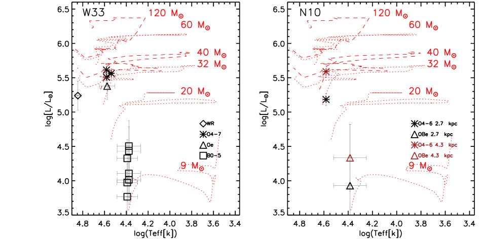
Figure 6.— Luminosity versus T_eff diagram of massive O-type stars (O4-6 and O6-7), B0-5 stars, and of the WN6b star detected in the direction of W33 (left) and of N10 (right). For W33, we assume a distance of 2.4 kpc; for N10, the same two stars are plotted for a distance of 2.4 kpc (black points) and for a distance of 4.3 kpc (lighter points). Stellar tracks for stars of 9, 20, 32, 40, 60, and 120 M_⊙, with solar metallicity and including rotation, are shown with dotted and dashed curves (Ekström et al. 2012).

At the position of Oe star #22, the SINFONI cube shows several H₂ lines, suggesting that star #22 (K_s=10.448 mag) is still embedded. We derived A${}_{\rm K_{\rm s}}$=$2.87\pm 0.07$ mag from the $J-H$ color excess; by assuming a distance of 2.4 kpc, we estimate M_K=$-4.33\pm 0.18$ mag. For confirming its luminosity class, further spectroscopy in $J$ and $H$-band is required.

5.2. A new WN6

Found in the south-west periphery of W33 (as shown in Fig. 7), the WN6b star #1 has an A${}_{\rm K_{\rm s}}$=1.0 mag, when assuming the average intrinsic near-infrared colors for late WN stars by Crowther et al. (2006a). With a distance of 2.4 kpc we measured $M_{K}=-4.86\pm 0.16$ mag, which fits well with the average $M_{K}=-5.13$ mag ($\sigma=0.07$ mag) of two other WN6b stars analyzed by Crowther et al. (2006a). By using BC_K=$-3.5\pm 0.5$ mag we obtain log(L/L_⊙)=$5.24^{+0.21}_{-0.21}$, and a mass of about $27\pm 2.5$ M_⊙. The detection of a late WN implies the existence of highly luminous progenitor supergiants (Georgy et al. 2012), such as those we detected in Mercer1.

The compilations of Galactic WR stars by van der Hucht (2001), Mauerhan et al. (2011), Shara et al. (2012), and Faherty et al. (2014), identify 43 WN6 stars from a total of 443 WRs of all flavours. Among the 12 WN6 stars listed in the latter three works 40% have broad features, suggesting that only 4% of known WRs have a similar classification. Rapid rotation and the presence of a magnetic field have been suggested to explain the broadening of their spectral lines and the flattening of the line peaks (Shenar et al. 2014).

5.3. Spectral types B0-5

Six B0-5 stars were detected. Stars #3, #4, #6, #10, and #13 are located in the Mercer1 region, with A${}_{\rm K_{\rm s}}$ values of $1.47\pm 0.04$ mag, $1.27\pm 0.03$ mag, $1.25\pm 0.21$ mag, $1.98\pm 0.02$ mag, and $1.07\pm 0.02$ mag, respectively. For a distance of 2.4 kpc, their M_K values range from $-2.07$ mag to $-3.69$ mag, and suggest a mix of dwarfs and giants (Martins & Plez 2006; Humphreys & McElroy 1984; Wegner 1994; Lejeune & Schaerer 2001) with initial masses from 9 to 15 M_⊙ (Ekström et al. 2012).

The B0-5 stars #18 and #17 are located in the cl2 cluster. Star #18 is the brightest star in the small cluster. For a distance of 2.4 kpc, it has A${}_{\rm K_{\rm s}}$=$1.66\pm 0.02$ mag and M_K$=-2.96\pm 0.16$ mag, which suggests a luminosity class V/III and an initial mass of $12\pm 3$ M_⊙ (Ekström et al. 2012). Star #17, with A${}_{\rm K_{\rm s}}$=$1.83\pm 0.01$ mag and M_K=$-1.56\pm 0.16$ mag, has a likely initial mass of $10\pm 2$ M_⊙.

We note that the nine stars generically classified as ‘early’ (i.e., those assigned spectral type OBAF in Table 1) exhibit such an uncertainty in temperatures and hence intrinsic colours that we cannot derive meaningful physically properties for them at this time.

5.4. Late-type Stars

For a distance of 2.4 kpc, the detected late-type stars from Table 3 remain fainter than M_bol=$-$5.26 mag (log(L/L_⊙)=4.0). They all have magnitudes consistent with those of giant stars.

6. The global structure and star formation history of W33

Complementing Fig. 1, in which we show the location of (candidate) massive stars in the putative individual clusters, Fig. 7 delineates the nominal locations of these regions on a map of the 8 $\mu$m  emission. Massive stars are found throughout W33, with the richest region being the Mercer 1 aggregate to the west of W33 Main. The presence of two O4-6 (super-)giants #7 and #8 suggests a burst of star formation occurred $\sim 2-4$ Myr ago. A further five early to mid B-type stars (#3, #4, #6, #10, and #13) have A${}_{\rm K_{\rm s}}$ consistent with those of the O-type stars and bolometric magnitudes typical of dwarfs and/or giants. The remaining three stars (#2, #5, and #9) are of generic early (OBAF) spectral-type.

Immediately to the west of Mercer 1 and the embedded protocluster forming within the radio source W33 Main, we find the O4-6 (super-)giant #23, which demonstrates similar physical properties to stars #7 and #8. In GLIMPSE images, star #23 is surrounded by a yellow curved filament, similar to the mid-infrared bow shocks identified by Povich et al. (2008). The likely young massive Oe star #22 is located in front of the apex of the bowshock between #23 and the radio source W33 Main, consistent with it’s elevated extinction (A${}_{\rm K_{\rm s}}$=$2.87\pm 0.07$ mag). The lack of further massive stars in this region leads us to conclude that the cl1 region does not delineate a bona fide cluster.

The massive protostar W33A (Davies et al. 2010) is located in the north-east of these regions, while the stellar aggregate cl2 is located to the south. A sequence of reddened stars is detected within the compact nebula of cl2 (Fig. 1 and Fig. 8); these are found at $J-$K_s$\approx 1.6$ mag in the color magnitude diagram shown in Fig. 8. The two brightest stars, #17 and #18, are spectroscopic B0-5 types, while the remaining three, #19, #20 and #21, are classified as spectral type OBAF. Radio continuum emission is found in the direction of the cl2 cluster, centered on star #18; we estimate a flux density of 0.57 Jy at 20 cm, and 0.64 Jy at 90 cm by using MAGPIS data and an aperture of 35^′′. Under the assumption of optically thin thermal emission with an electron temperature, T_e=10,000 K, this implies a Lyman continuum photon flux, N_lyc, of 10^47.2 s^-1 (e.g., Martín-Hernández et al. 2003; Rubin 1968; Storey & Hummer 1995). For comparison, a O9.5 V emits a number of N_lyc of $10^{47.9}$ s^-1 and a O9.5 III of $10^{48.4}$ s^-1 (from the more recent work by Martins et al. 2005). By comparing the results from Martins et al. (2005), Vacca et al. (1996), and Panagia (1973), after having corrected for relative average shifts, we estimate N_lyc=10^47.2 s^-1, 10^48.0 s^-1, 10^44.4 s^-1, and 10^45.1 s^-1 for a B0 V, a B0 III, a B2 V, and a B2 III star, respectively. We find typical uncertainties of 0.2 dex for every N_lyc value. Therefore, stars #17 and #18 may already account for the requisite ionising flux. While early B-type stars with initial masses of 9-12 M_⊙ are present in stellar populations with ages ranging up to 30 Myr (Ekström et al. 2012), the nebular emission associated with cl2 suggests a much younger age, likely of only a few Myr.

Finally, further to the south-west we find the broad lined WN6 star #1. We unsuccessfully searched the W33 area for other possible bright stars (K_s$<10$ mag) with properties of free-free emitters or candidate red supergiants by using the infrared photometric criteria of Messineo et al. (2012). Thus, it is unlikely that there are any further young massive stellar aggregates associated with the complex. Consideration of these findings emphasizes that the massive stellar population is distributed across the confines of the W33 and appears not to be concentrated in rich young clusters similar to e.g., Danks 1 and Danks 2 within the G305 star forming complex (Davies et al. 2012).

This behavior appears to mirror the current location of cold molecular material, within which future generations of stars may form. Immer et al. (2014) report the detection of six molecular clumps along the east side of W33, with masses of $0.2-4.0\times 10^{3}$ M_⊙  coincident with the peak of the CO intensity map (see Figure 7). By contrast the evolved H II region G12.745-00.153 (Mercer1) resides on the west side of W33, where the molecular matter has already been swept out, a configuration that is at least suggestive of sequential star formation. Similarly the dense clump W33B1 (Immer et al. 2014) is located $\sim 35$^′′ South-West of the cl2 cluster on the periphery of the apparent wind blown nebula associated with the latter; it is conceivable that its influence is contributing to this new protostellar core by heating and compressing it (Immer et al. 2014).

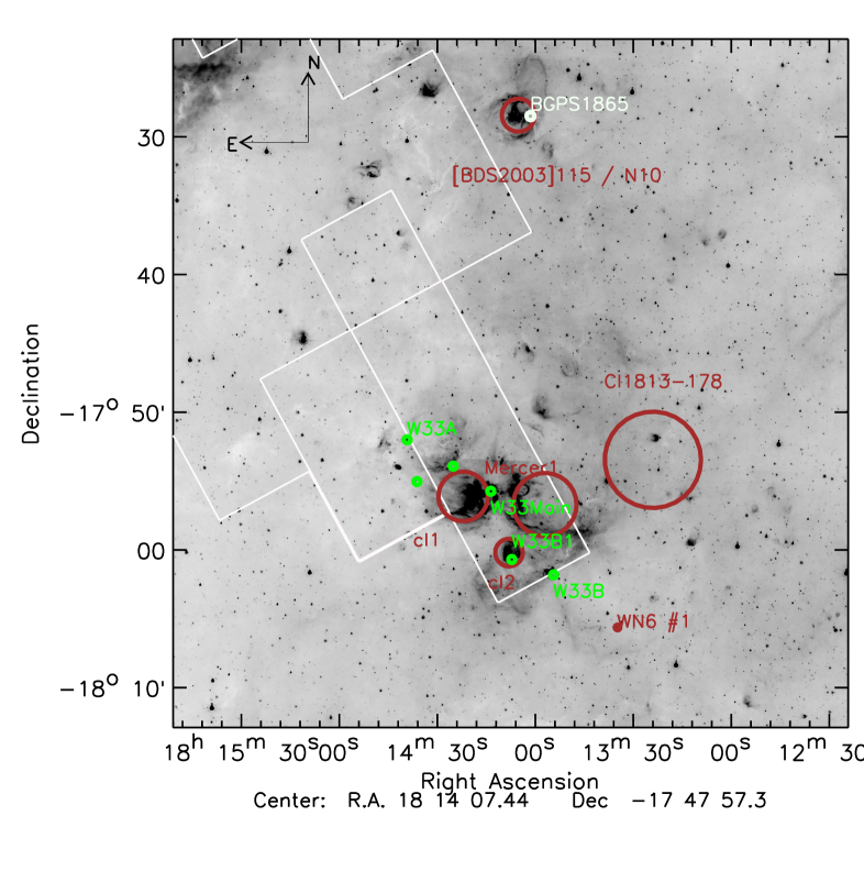
Figure 7.— 8 $\mu$m emission from GLIMPSE (Churchwell et al. 2009) of W33. The Mercer1, cl1, cl2 and Cl1813$-$178 regions are marked with circles, as well as the isolated WN6 star #1. The green dots indicate the location of the molecular clumps in W33 detected by Immer et al. (2014), and in blue that in N10 studied by Ma et al. (2013). The white contours show the location of the peak of ¹²CO emission in the range from 30 km s^-1 to 60 km s^-1 from the Galactic survey of Dame et al. (2001). The image has a linear size of 34.5 pc $\times$ 35.09 pc for a distance of 2.4 kpc.

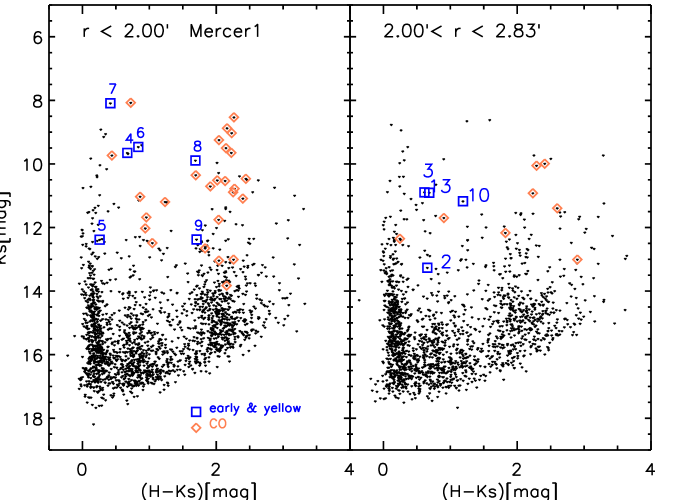
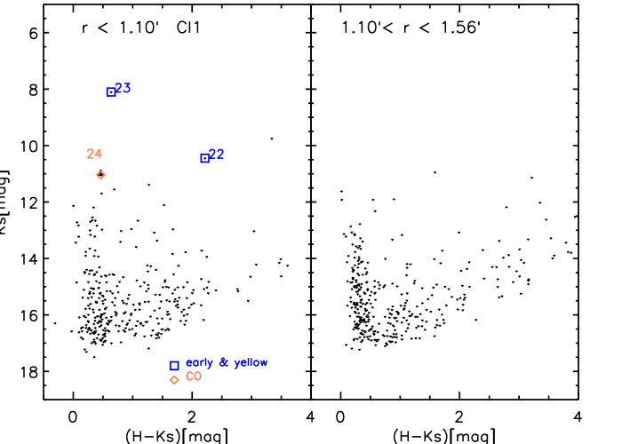
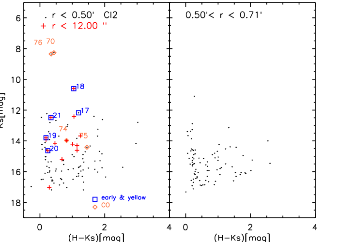
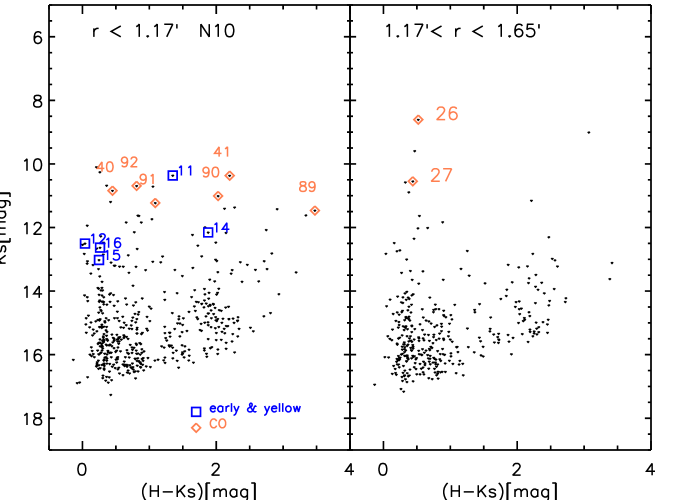
Figure 8.— 2MASS-UKIDSS $H-$K_s versus K_s diagram of the Mercer1 (top left), cl1 (top right), cl2 (bottom left ), and N10 (bottom right ) regions. Spectroscopic detected early-yellow stars are indicated with squares, late-type stars with diamonds. Identification numbers are taken from Tables 1 and 3. A comparison field of equal area is shown in the right panel; field datapoints are taken from an annular region. In the cl2 region, stars concentrated in the central 12^′′ are marked with crosses.

Table 5 Physical properties of newly detected massive stars.

IDb	Sp.	Classc	Teff	$K_{\mathrm{S}_{o}}$	A${}_{\rm K_{\rm s}}$	$BC_{\mathrm{K}_{S}}$	$M_{K_{\mathrm{S}}}$(der.)	${\mathrm{l}og}(L/\hbox{\it L${}_{\odot}$})$	Region
			[K]	[mag]	[mag]	[mag]	[mag]	[mag]
1	WN6	I	70000$\pm$ 5000	7.043 $\pm$ 0.033	0.981 $\pm$ 0.025	$-$3.50 $\pm$ 0.50	$-$4.86 $\pm$ 0.16	$5.24^{+0.21}_{-0.21}$	South of W33
3	B0$-$5	III	24000$\pm$ 6700	9.437 $\pm$ 0.059	1.470 $\pm$ 0.040	$-$2.83 $\pm$ 0.87	$-$2.46 $\pm$ 0.17	$4.01^{+0.35}_{-0.35}$	Mercer1, W33
4	B0$-$5	III	24000$\pm$ 6700	8.386 $\pm$ 0.035	1.267 $\pm$ 0.025	$-$2.83 $\pm$ 0.87	$-$3.52 $\pm$ 0.16	$4.43^{+0.35}_{-0.35}$	Mercer1, W33
6	B0$-$5	III	24000$\pm$ 6700	8.212 $\pm$ 0.245	1.254 $\pm$ 0.208	$-$2.83 $\pm$ 0.87	$-$3.69 $\pm$ 0.29	$4.50^{+0.37}_{-0.37}$	Mercer1, W33
7	O4$-$6	I	38000$\pm$ 2500	7.271 $\pm$ 0.057	0.819 $\pm$ 0.051	$-$4.40 $\pm$ 0.15	$-$4.63 $\pm$ 0.17	$5.51^{+0.09}_{-0.09}$	Mercer1, W33
8	O4$-$6	I	38000$\pm$ 2500	7.009 $\pm$ 0.067	2.883 $\pm$ 0.058	$-$4.40 $\pm$ 0.15	$-$4.89 $\pm$ 0.17	$5.61^{+0.09}_{-0.09}$	Mercer1, W33
10	B0$-$5	III	24000$\pm$ 6700	9.207 $\pm$ 0.020	1.978 $\pm$ 0.015	$-$2.83 $\pm$ 0.87	$-$2.69 $\pm$ 0.16	$4.11^{+0.35}_{-0.35}$	Mercer1, W33
13	B0$-$5	V	25000$\pm$ 5900	9.827 $\pm$ 0.026	1.067 $\pm$ 0.016	$-$3.12 $\pm$ 0.66	$-$2.07 $\pm$ 0.16	$3.97^{+0.27}_{-0.27}$	Mercer1, W33
17	B0$-$5	V	25000$\pm$ 5900	10.343 $\pm$ 0.021	1.832 $\pm$ 0.013	$-$3.12 $\pm$ 0.66	$-$1.56 $\pm$ 0.16	$3.77^{+0.27}_{-0.27}$	cl2, W33
18	B0$-$5	V	25000$\pm$ 5900	8.946 $\pm$ 0.023	1.657 $\pm$ 0.015	$-$3.12 $\pm$ 0.66	$-$2.96 $\pm$ 0.16	$4.33^{+0.27}_{-0.27}$	cl2, W33
22	Oe	$..$	$..$	7.576 $\pm$ 0.075	2.872 $\pm$ 0.071	$..$	$-$4.33 $\pm$ 0.18	$..$	cl1, W33
23	O6$-$7	I	35000$\pm$ 1200	6.904 $\pm$ 0.037	1.199 $\pm$ 0.027	$-$4.17 $\pm$ 0.08	$-$5.00 $\pm$ 0.16	$5.56^{+0.07}_{-0.07}$	cl1, W33
11	O4-6	I	38000$\pm$ 2500	8.083 $\pm$ 0.039	2.280 $\pm$ 0.032	-4.40 $\pm$ 0.15	-5.08 $\pm$ 0.10	$5.69^{+0.07}_{-0.07}$	BDS2003-115
14	OBe	$..$	$..$	9.691 $\pm$ 0.028	2.465 $\pm$ 0.026	$..$	$-$3.47 $\pm$ 0.10	$..$	BDS2003-115

• A distance of $2.4^{+0.17}_{-0.15}$ kpc (DM = $+11.90\pm 0.16$ mag) is used for W33 (Immer et al. 2013), and of $4.29^{0.17}_{-0.19}$ kpc (DM = $13.16\pm 0.09$ mag) for N10. (^b) OBAF detections are not included in this table. (^c) Classes are photometrically estimated using M_K values from Martins & Plez (2006), Bibby et al. (2008), Humphreys & McElroy (1984), and Lejeune & Schaerer (2001).

7. BDS2003-115 and Bubble N10

The cluster candidate BDS2003-115 is located North of W33 (Bica et al. 2003; Messineo et al. 2011). It appears as a group of bright near-infrared stars in the core of a mid-infrared bubble (bubble N10, and candidate SNR G13.1875+0.0389, Helfand et al. 2006; Watson et al. 2008; Churchwell et al. 2006). Radio line observations of the ¹³CO $J=3-2$ transition yielded a radial velocity V_LSR= $50.2\pm 4.1$ km s^-1  (Beaumont & Williams 2010). We calculated the distance to N10 using the Galactic rotation curve parameters determined by Reid et al. (2009) from fitting trigonometric parallaxes of star forming regions, i.e., $R_{\odot}=8.4\pm 0.6$ kpc and $\Theta_{0}=254\pm 16$ km s^-1. We find a distance of 4.29${}^{+0.17}_{-0.19}$ kpc. This could correspond to the high-velocity component seen in direction of W33; the low-velocity component of W33 (35 km s^-1) is also detected along the line-of-sight of N10 (Dame et al. 2001). Bubble N10 is among the 28% of bubbles currently interacting with a molecular condensation (Deharveng et al. 2010); this clump (hereafter, BGPS1865) is locate on the western edge of the bubble and has a mass ($>1600$ M_⊙) (Ma et al. 2013, and references therein).

We detected one O4-6 star (star #11, A${}_{\rm K_{\rm s}}$=$2.28\pm 0.03$ mag) in the center of the bubble N10, as well as 3 early type-stars (spectral-type OBAF; #12, #15, and #16) and the embedded massive star #14. For a distance of 2.4 kpc, we obtain M_K=$-4.07\pm 0.1$ mag for #11 (which is a typical value for dwarfs of $29\pm 3$ M_⊙, Martins & Plez 2006; Ekström et al. 2012); for a kinematic distance of 4.29 kpc this is revised upwards to M_K=$-5.08\pm 0.1$ mag ((super-)giant of $36\pm 4$ M_⊙, Martins & Plez 2006; Ekström et al. 2012). There is a hint for Si IV in emission at 2.428 $\mu$m in the spectrum of star #11. Given the uncertainty in reddening and temperature of the remaining 4 stars we are unable to determine their luminosities.

8. The relationship between Cl1813$-$178 and W33

The young massive cluster, Cl 1813$-$178 is projected onto the north-west periphery of W33, and is coincident with SNR G12.72$-$0.00 (e.g., Helfand et al. 2006; Brogan et al. 2006; Messineo et al. 2008, 2011). Messineo et al. also suggested a possible association of this cluster, with G12.83$-$0.02, and the pulsar and TeV Gamma-Ray Source PSR J1813$-$1749/HESS J1813$-$178 (Brogan et al. 2005).

The cluster contains six spectroscopically detected late O-type stars, twelve early B-type stars, two WN7 stars, and three transitional objects (the O6O7If star #5, the O8O9If #16, and the cLBV #15 in Messineo et al. 2011). Messineo et al. (2011) estimated a spectrophotometric distance of $3.7\pm 1.7$ kpc, consistent within errors with a stellar kinematic distance of $4.8\pm 0.2$ kpc, which is based on the radial velocity of the RSG member (V_LSR= $62\pm 4$ km s^-1, Messineo et al. 2008) and on the Galactic rotation parameters presented by Reid et al. (2009).

Given our current understanding of stellar evolution, it appears difficult to reconcile the distance of Cl 1813$-$178 with the new parallactic distance to the W33 complex ($\sim 2.4$ kpc). On the basis of the spectral features, luminosity classes can be inferred only for the transitional objects, the two WRs, and two other B0-B3 stars with He I at 2.058 $\mu$m in emission. While the magnitudes of O7-O9 stars and B0-B3 stars are consistent with both distances of 4.8 kpc and 2.4 kpc, the shorter distance would lead to extremely low luminosities for the three transitional objects, as shown in Table 6. For example, for the O6-O7If star, M_K=$-5.87\pm 0.11$ mag at 4.8 kpc or $-4.36\pm 0.17$ mag at 2.4 kpc; the latter value is not compatible with the supergiant class. The spectrum of O6-O7If star resembles that of star F15 in the Arches cluster (Martins et al. 2008); for F15 we derive M_K=$-5.76$ mag by using the photometry by Figer et al. (2002), the extinction law by Messineo et al. (2005), and a distance of 8.4 kpc. Thereby, the O6-O7If star must be located behind the W33 complex.

Furthermore, for a distance of 2.4 kpc, the cluster members of spectral type O or B would have initial masses below 25 M_⊙, i.e., below the theoretical and observed lower mass limit for the progenitors of late WN stars (Georgy et al. 2012; Messineo et al. 2011). As a consequence it would be difficult to understand the presence of the two WN7 (#4, #7 in Messineo et al. 2011), one O8-9If/WN9h, and one O6-O7If star, given the resultant absence of a progenitor population. The average M_K= $-5.86$ mag ($\sigma=0.43$ mag) inferred for the two WN7, cluster members, at 4.8 kpc is consistent with that of WN7 stars ($-5.38$ mag with a $\sigma=0.38$ mag) in Westerlund 1 (Crowther et al. 2006a).

Table 6 Average M_K, A${}_{\rm K_{\rm s}}$, and number of stars per spectral group and luminosity class in Cl 1813-178 (Table2, Messineo et al. 2011).

		Cluster distance(a) 4.8 kpc			W33 distance(b) 2.4 kpc
Sp. group	class(c)	MK(d)	A${}_{\rm K_{\rm s}}$(d)	Nstar	MK(d)	A${}_{\rm K_{\rm s}}$(d)	Nstar
B0-B3	I	$-6.32\pm 1.01$	$0.94\pm 0.25$	7	$-5.78\pm 0.33$	$0.87\pm 0.18$	3
B0-B3	V/III	$-4.24\pm 0.60$	$0.98\pm 0.34$	5	$-3.32\pm 0.90$	$0.97\pm 0.30$	9
O7-O9	I	$-5.48\pm 0.28$	$0.84\pm 0.09$	5	$..$	$..$	0
O7-O9	V/III	$-4.93\pm 0.11$	$0.86\pm 0.02$	1	$-3.88\pm 0.36$	$0.83\pm 0.09$	6
WN7	I	$-5.86\pm 0.43$	$0.75\pm 0.08$	2	$-4.35\pm 0.43$	$0.75\pm 0.08$	2
O6O7If	I	$-5.87\pm 0.11$	$1.03\pm 0.02$	1	$-4.36\pm 0.17$	$1.03\pm 0.02$	1
O8O9If	I	$-7.32\pm 0.10$	$1.24\pm 0.01$	1	$-5.81\pm 0.16$	$1.24\pm 0.01$	1
cLBV	I	$-7.53\pm 0.10$	$1.09\pm 0.02$	1	$-6.03\pm 0.16$	$1.09\pm 0.02$	1

• ^(a) Cluster kinematic distance (Messineo et al. 2008; Reid et al. 2009).  ^(b) W33 distance (Immer et al. 2013).  ^(c) Luminosity classes are photometrically assigned: for B0-B3 supergiants M_K $<-5.0$ mag, for B0-B3 giants or dwarfs M_K $>-5.0$ mag. For O7-O9 supergiants M_K $<-5.0$ mag, for O7-O9 giants or dwarfs M_K $>-5.0$ mag. ^(d) When Nstar $>1$, quoted errors are the standard deviations.

While the SN that gave rise to the remnant G12.72$-$0.00 may have occurred in Cl 1813$-$178 (given the precise superposition), a physical association with SNR G12.82$-$0.02 and associated pulsar PSR J1813$-$1749 appears doubtful. Specifically, a comparison of the significant column density to the pulsar and SNR to the less extreme extinction inferred for cluster members led Halpern et al. (2012) to conclude that SNR G12.82$-$0.02 likely lies beyond both the cluster and the W33 complex ($d\sim 5-12$ kpc).

Finally, it is of interest that the distance estimate for the W33 complex was determined from parallax measurement of masers. If it were to be observed in the future, when such emission had ceased, it would be difficult to recognize it as a complex of discrete sources at the same distance, and to further distinguish the distinct stellar population of Cl1813$-$178 that is projected on the edge of W33 (see Fig. 7).

9. Summary

We performed a near-IR spectroscopic survey for massive stars, encompassing both W33 and the nearby mid-IR bubble/stellar cluster N10/BDS2003-115 to study their star formation history.

• We detected a total of fourteen new early-type (OB and WR) stars and a further nine stars with spectra consistent with spectral types earlier than F. A large population of giants with spectral types G-M were uncovered, but no cool supergiants associated with W33 were identified.

• Following Clark et al. (2009b), the lack of RSGs precludes substantive star formation activity with W33 $\geq 6$ Myr, while the detected stellar population appears broadly consistent with an age of $\sim 2-4$ Myr.

• The complex contains protostars (most notably the embedded protocluster W33 Main and the high mass protostar W33A), massive evolved stars, and clear marks of sequential star formation and feedback. Star formation within W33 has not led to the formation of rich dense clusters, and the size of W33 (radius $\approx 5$ pc) is typical for loose associations (Pfalzner 2009). When the GMC is exhausted and star formation has ceased, W33 will most likely resemble a loose, non-coeval stellar association similar to (but less massive than) Cyg OB2 (e.g., Negueruela et al. 2008).

• Given the spare nature of individual stellar ‘aggregates’ and the limitations of the current data, we cannot infer integrated masses for the young populations within W33. W33 is probable less massive than other massive star forming complexes of the Milky Way with known evolved stars, such as W43 (e.g., Blum et al. 1999; Chen et al. 2013), W51 (Clark et al. 2009b), Carina (e.g., Preibisch et al. 2011), and G305 (Davies et al. 2012), as suggested by their respective integrated radio and IR luminosities (e.g., Immer et al. 2013; Conti & Crowther 2004).

• The greater distance to the nearby young massive stellar aggregate Cl 1813$-$178 precludes a physical association with W33. The late O-type and B-type members of the cluster support a distinct older population than that observed in W33. Considering the extinction of Cl 1813$-$178 (A_V=9.1 mag), optical spectroscopy would yield precise spectral-types and direct luminosity determinations for its constituent stars (e.g, Negueruela et al. 2010).

• Given the distances to W33 and to Cl 1813$-$178, an association with the energetic pulsar PSR J1813$-$1749 appears doubtful.

Table 7 Infrared measurements of the spectroscopically detected stars. Identification numbers are taken from Table 1, 3.

	2MASS			DENIS			UKIDSS			GLIMPSE					MSX	WISE		NOMAD
ID	J	H	$K_{S}$	I	J	$K_{S}$	J	H	$K$	Flag	[3.6]	[4.5]	[5.8]	[8.0]	A	W1	W2	R
	[mag]	[mag]	[mag]	[mag]	[mag]	[mag]	[mag]	[mag]	[mag]		[mag]	[mag]	[mag]	[mag]	[mag]	[mag]	[mag]	[mag]
1	10.168	8.887	8.024	13.969	10.053	8.059	$\cdots$	$\cdots$	$\cdots$	2	7.247	6.686	6.520	6.192	$\cdots$	$\cdots$	$\cdots$	$\cdots$
2	15.364	$\cdots$	$\cdots$	$\cdots$	15.171	12.121	15.252	13.922	13.266	1	$\cdots$	$\cdots$	$\cdots$	$\cdots$	$\cdots$	$\cdots$	$\cdots$	$\cdots$
3	13.230	11.658	10.913	$\cdots$	13.203	10.831	13.267	11.592	10.907	1	10.364	10.462	10.058	$\cdots$	$\cdots$	10.631	10.170	$\cdots$
4	11.756	10.324	9.653	16.440	11.561	9.668	11.561	10.231	9.500	2	9.008	8.893	8.686	8.493	$\cdots$	9.050	8.896	$\cdots$
5	13.018	$\cdots$	$\cdots$	14.124	13.120	$\cdots$	13.032	12.640	12.383	1	$\cdots$	$\cdots$	$\cdots$	$\cdots$	$\cdots$	$\cdots$	$\cdots$	14.45
6	$\cdots$	$\cdots$	$\cdots$	$\cdots$	$\cdots$	$\cdots$	11.718	10.301	9.466	1	$\cdots$	$\cdots$	$\cdots$	$\cdots$	$\cdots$	$\cdots$	$\cdots$	$\cdots$
7	9.376	8.508	8.090	12.117	9.457	8.008	9.389	$\cdots$	$\cdots$	2	7.737	7.764	7.661	7.730	$\cdots$	$\cdots$	$\cdots$	14.07
8	14.913	11.581	9.892	$\cdots$	14.629	9.734	15.104	11.675	9.805	2	8.588	8.296	7.955	8.126	$\cdots$	8.627	8.056	$\cdots$
9	$\cdots$	13.858	$\cdots$	$\cdots$	$\cdots$	$\cdots$	17.322	14.083	12.377	1	$\cdots$	$\cdots$	$\cdots$	$\cdots$	$\cdots$	$\cdots$	$\cdots$	$\cdots$
10	$\cdots$	$\cdots$	$\cdots$	$\cdots$	$\cdots$	$\cdots$	14.697	12.416	11.185	1	$\cdots$	$\cdots$	$\cdots$	$\cdots$	$\cdots$	$\cdots$	$\cdots$	$\cdots$
11	$\cdots$	11.713	10.363	$\cdots$	$\cdots$	10.249	14.325	11.703	10.278	2	9.401	9.127	8.835	$\cdots$	$\cdots$	$\cdots$	$\cdots$	$\cdots$
12	$\cdots$	$\cdots$	$\cdots$	13.372	12.081	$\cdots$	12.907	12.543	12.505	1	$\cdots$	$\cdots$	$\cdots$	$\cdots$	$\cdots$	$\cdots$	$\cdots$	$\cdots$
13	12.718	11.524	10.826	16.555	12.634	10.698	12.681	11.507	10.894	1	$\cdots$	$\cdots$	$\cdots$	$\cdots$	$\cdots$	$\cdots$	$\cdots$	$\cdots$
14	$\cdots$	$\cdots$	12.224	$\cdots$	$\cdots$	$\cdots$	16.918	14.036	12.156	1	10.408	9.677	10.118	$\cdots$	$\cdots$	9.428	8.128	$\cdots$
15	13.995	13.189	$\cdots$	15.927	13.880	12.056	14.006	13.271	13.023	1	$\cdots$	$\cdots$	$\cdots$	$\cdots$	$\cdots$	$\cdots$	$\cdots$	17.07
16	13.535	12.944	$\cdots$	15.439	13.374	$\cdots$	13.538	12.896	12.633	1	$\cdots$	$\cdots$	$\cdots$	$\cdots$	$\cdots$	$\cdots$	$\cdots$	16.85
17	15.411	13.290	12.102	$\cdots$	14.942	11.975	15.454	13.367	12.175	1	11.305	$\cdots$	$\cdots$	$\cdots$	$\cdots$	$\cdots$	$\cdots$	$\cdots$
18	13.457	11.652	10.567	18.408	13.375	10.523	13.526	11.648	10.603	1	$\cdots$	$\cdots$	$\cdots$	$\cdots$	$\cdots$	$\cdots$	$\cdots$	$\cdots$
19	14.654	13.826	13.053	16.450	14.639	$\cdots$	14.699	13.984	13.797	1	$\cdots$	$\cdots$	$\cdots$	$\cdots$	$\cdots$	$\cdots$	$\cdots$	16.72
20	15.044	14.084	12.918	16.900	14.915	$\cdots$	15.502	14.881	14.638	1	$\cdots$	$\cdots$	$\cdots$	$\cdots$	$\cdots$	$\cdots$	$\cdots$	$\cdots$
21	13.531	12.692	11.914	15.770	13.464	11.944	13.538	12.829	12.488	1	$\cdots$	$\cdots$	$\cdots$	$\cdots$	$\cdots$	$\cdots$	$\cdots$	17.07
22	15.983	12.664	10.448	$\cdots$	$\cdots$	10.569	15.421	12.369	10.072	2	8.006	7.283	6.627	5.962	$\cdots$	7.868	6.766	$\cdots$
23	10.062	8.741	8.103	14.030	9.997	8.091	9.846	$\cdots$	7.946	2	7.604	7.493	7.466	$\cdots$	$\cdots$	$\cdots$	$\cdots$	16.65
24	12.724	11.505	10.986	15.478	12.838	10.989	12.724	11.500	11.036	1	$\cdots$	$\cdots$	$\cdots$	$\cdots$	$\cdots$	$\cdots$	$\cdots$	17.10
25	$\cdots$	13.023	10.989	$\cdots$	$\cdots$	10.989	17.218	12.996	10.970	1	9.636	9.516	9.148	9.356	$\cdots$	9.342	9.077	$\cdots$
26	10.318	9.128	8.607	13.144	10.164	8.545	10.278	$\cdots$	8.652	2	8.323	8.362	8.160	8.200	$\cdots$	8.425	8.419	15.18
27	12.089	10.985	10.546	14.682	11.923	10.514	12.059	10.960	10.592	2	10.232	10.385	9.741	9.343	$\cdots$	10.251	9.900	16.17
28	$\cdots$	11.343	10.069	$\cdots$	14.130	10.280	$\cdots$	$\cdots$	$\cdots$	2	9.197	9.273	8.896	8.929	$\cdots$	9.232	9.126	$\cdots$
29	$\cdots$	13.950	12.888	$\cdots$	$\cdots$	$\cdots$	16.656	14.289	13.069	3	12.040	12.072	11.984	$\cdots$	$\cdots$	$\cdots$	$\cdots$	$\cdots$
30	14.448	11.369	9.839	$\cdots$	14.534	9.825	$\cdots$	$\cdots$	$\cdots$	2	8.694	8.764	8.320	8.301	$\cdots$	9.002	8.648	$\cdots$
31	$\cdots$	12.221	9.892	$\cdots$	$\cdots$	9.827	16.645	12.221	9.796	2	8.197	8.104	7.627	7.768	$\cdots$	8.452	8.040	$\cdots$
32	14.969	11.788	$\cdots$	$\cdots$	14.681	10.123	15.392	11.835	10.081	2	$\cdots$	$\cdots$	$\cdots$	$\cdots$	$\cdots$	$\cdots$	$\cdots$	$\cdots$
33	$\cdots$	13.074	10.931	$\cdots$	$\cdots$	11.053	17.542	13.155	10.921	1	9.415	9.390	8.896	9.114	$\cdots$	9.651	9.325	$\cdots$
34	13.342	$\cdots$	$\cdots$	15.133	13.105	10.772	13.464	12.651	12.363	1	$\cdots$	$\cdots$	$\cdots$	$\cdots$	$\cdots$	$\cdots$	$\cdots$	16.69
35	$\cdots$	$\cdots$	$\cdots$	$\cdots$	$\cdots$	$\cdots$	$\cdots$	14.043	11.403	1	$\cdots$	$\cdots$	$\cdots$	$\cdots$	$\cdots$	9.429	9.049	$\cdots$
36	$\cdots$	$\cdots$	$\cdots$	$\cdots$	$\cdots$	$\cdots$	$\cdots$	15.959	13.018	1	$\cdots$	$\cdots$	$\cdots$	$\cdots$	$\cdots$	$\cdots$	$\cdots$	$\cdots$
37	$\cdots$	12.807	10.785	$\cdots$	$\cdots$	$\cdots$	16.846	13.052	10.779	1	9.256	9.128	8.682	8.898	$\cdots$	9.315	8.845	17.20
38	$\cdots$	12.477	10.530	$\cdots$	$\cdots$	10.431	$\cdots$	12.532	10.516	1	9.111	9.032	8.567	8.698	$\cdots$	9.363	9.007	$\cdots$
39	12.522	11.127	10.530	16.098	12.530	10.516	12.461	11.216	10.489	3	10.056	10.088	9.952	$\cdots$	$\cdots$	10.334	10.153	$\cdots$
40	12.236	11.290	10.841	$\cdots$	$\cdots$	10.802	12.283	11.310	10.965	2	$\cdots$	$\cdots$	$\cdots$	$\cdots$	$\cdots$	$\cdots$	$\cdots$	$\cdots$
41	$\cdots$	12.569	10.368	$\cdots$	$\cdots$	10.386	17.008	12.560	10.313	2	8.750	8.632	8.171	8.274	$\cdots$	8.903	8.198	$\cdots$
42	13.305	10.899	9.761	$\cdots$	$\cdots$	9.855	$\cdots$	$\cdots$	$\cdots$	2	8.978	9.152	8.785	8.892	$\cdots$	9.042	9.091	$\cdots$
43	12.808	10.941	10.124	17.603	12.943	10.083	$\cdots$	$\cdots$	$\cdots$	2	9.557	9.538	9.405	9.470	$\cdots$	9.595	9.665	$\cdots$
44	13.968	11.433	10.026	$\cdots$	14.263	10.288	$\cdots$	$\cdots$	$\cdots$	2	8.799	8.553	8.178	7.981	$\cdots$	8.606	8.202	$\cdots$
45	14.392	12.009	10.893	$\cdots$	14.597	11.000	14.308	12.033	10.879	3	10.193	10.215	9.907	9.945	$\cdots$	$\cdots$	$\cdots$	$\cdots$
46	12.919	11.298	10.593	17.500	12.991	10.714	12.757	11.432	10.607	3	10.111	10.191	9.971	9.888	$\cdots$	10.195	10.227	$\cdots$
47	11.302	8.275	6.604	$\cdots$	12.227	7.338	$\cdots$	$\cdots$	$\cdots$	2	5.859	6.023	4.934	4.659	4.173	5.914	4.960	$\cdots$
48	$\cdots$	12.102	$\cdots$	$\cdots$	$\cdots$	10.448	15.308	12.232	10.695	3	$\cdots$	$\cdots$	$\cdots$	$\cdots$	$\cdots$	$\cdots$	$\cdots$	$\cdots$

• The Flag column indicates which $JHK$ was adopted in the paper: Flag=0 source missing; Flag=1 UKIDSS psf-fitting magnitudes; Flag=2 2MASS magnitudes; Flag=3 UKIDSS DR6 release.

Table 7 Continuation of Table 7.

	2MASS			DENIS			UKIDSS			GLIMPSE					MSX	WISE		NOMAD
ID	J	H	$K_{S}$	I	J	$K_{S}$	J	H	$K$	Flag	[3.6]	[4.5]	[5.8]	[8.0]	A	W1	W2	R
	[mag]	[mag]	[mag]	[mag]	[mag]	[mag]	[mag]	[mag]	[mag]		[mag]	[mag]	[mag]	[mag]	[mag]	[mag]	[mag]	[mag]
49	$\cdots$	12.343	10.054	$\cdots$	$\cdots$	9.894	16.907	12.242	9.911	2	8.469	8.309	7.934	8.103	$\cdots$	8.623	8.238	$\cdots$
50	$\cdots$	12.402	9.991	$\cdots$	$\cdots$	9.864	17.441	12.554	9.971	2	8.185	7.804	7.372	7.380	$\cdots$	8.345	7.507	$\cdots$
51	15.406	$\cdots$	$\cdots$	$\cdots$	15.207	8.948	15.483	11.260	9.029	1	$\cdots$	$\cdots$	$\cdots$	$\cdots$	$\cdots$	$\cdots$	$\cdots$	$\cdots$
52	$\cdots$	13.189	10.908	$\cdots$	$\cdots$	11.030	18.233	13.486	11.088	1	9.378	9.157	8.802	8.914	$\cdots$	9.656	9.153	$\cdots$
53	$\cdots$	12.879	10.554	$\cdots$	$\cdots$	10.341	17.624	12.909	10.466	1	8.842	8.678	8.213	8.258	$\cdots$	9.192	8.700	$\cdots$
54	$\cdots$	11.876	9.650	$\cdots$	16.250	9.491	16.570	11.990	9.599	2	8.104	7.997	7.471	7.575	$\cdots$	8.038	7.608	$\cdots$
55	$\cdots$	14.413	12.678	$\cdots$	$\cdots$	$\cdots$	18.239	14.487	12.653	1	11.443	11.259	11.026	$\cdots$	$\cdots$	$\cdots$	$\cdots$	$\cdots$
56	10.359	8.796	8.074	14.426	10.261	8.171	10.272	$\cdots$	8.390	2	7.647	7.861	7.551	7.584	$\cdots$	7.708	7.902	18.21
57	$\cdots$	10.797	8.532	$\cdots$	$\cdots$	$\cdots$	14.561	10.353	$\cdots$	2	6.713	5.976	5.456	5.432	5.965	6.669	5.790	$\cdots$
58	$\cdots$	$\cdots$	$\cdots$	$\cdots$	$\cdots$	$\cdots$	$\cdots$	15.267	13.008	1	$\cdots$	$\cdots$	$\cdots$	$\cdots$	$\cdots$	$\cdots$	$\cdots$	$\cdots$
59	$\cdots$	$\cdots$	$\cdots$	$\cdots$	$\cdots$	$\cdots$	$\cdots$	$\cdots$	11.213	1	8.730	8.409	7.943	7.922	$\cdots$	$\cdots$	$\cdots$	$\cdots$
60	10.983	10.173	9.733	12.567	11.113	9.816	10.938	10.119	9.976	2	$\cdots$	$\cdots$	$\cdots$	$\cdots$	$\cdots$	$\cdots$	$\cdots$	12.38
61	$\cdots$	11.646	9.500	$\cdots$	$\cdots$	9.332	16.123	11.743	9.392	2	7.871	7.812	7.317	7.462	$\cdots$	8.263	7.906	$\cdots$
62	$\cdots$	$\cdots$	$\cdots$	$\cdots$	$\cdots$	$\cdots$	15.359	11.039	8.877	1	$\cdots$	$\cdots$	$\cdots$	$\cdots$	$\cdots$	7.684	7.327	$\cdots$
63	$\cdots$	13.134	10.946	$\cdots$	$\cdots$	10.815	17.622	13.143	10.890	1	9.412	9.277	8.807	9.079	$\cdots$	9.682	9.328	$\cdots$
64	$\cdots$	$\cdots$	$\cdots$	$\cdots$	$\cdots$	$\cdots$	$\cdots$	15.078	13.038	1	$\cdots$	$\cdots$	$\cdots$	$\cdots$	$\cdots$	$\cdots$	$\cdots$	$\cdots$
65	$\cdots$	12.565	10.516	$\cdots$	$\cdots$	$\cdots$	16.647	12.667	10.534	1	9.065	8.912	8.525	8.784	$\cdots$	9.266	8.899	$\cdots$
66	$\cdots$	$\cdots$	$\cdots$	$\cdots$	$\cdots$	$\cdots$	$\cdots$	15.982	13.826	1	$\cdots$	$\cdots$	$\cdots$	$\cdots$	$\cdots$	$\cdots$	$\cdots$	$\cdots$
67	15.249	11.288	9.247	$\cdots$	15.581	9.271	15.312	11.562	9.341	2	7.967	7.485	7.035	7.010	$\cdots$	8.355	7.534	$\cdots$
68	$\cdots$	$\cdots$	10.766	$\cdots$	$\cdots$	10.654	16.547	12.617	10.705	1	9.434	9.310	8.951	8.993	$\cdots$	$\cdots$	$\cdots$	$\cdots$
69	$\cdots$	$\cdots$	12.400	$\cdots$	$\cdots$	$\cdots$	15.949	13.533	12.488	1	11.679	11.694	$\cdots$	$\cdots$	$\cdots$	$\cdots$	$\cdots$	$\cdots$
70	9.863	8.703	8.271	12.260	9.801	8.243	9.689	$\cdots$	8.248	2	$\cdots$	$\cdots$	$\cdots$	$\cdots$	$\cdots$	$\cdots$	$\cdots$	14.59
71	12.300	9.616	8.313	$\cdots$	12.316	8.424	$\cdots$	$\cdots$	$\cdots$	2	7.347	7.563	7.112	7.140	$\cdots$	7.551	7.476	$\cdots$
72	$\cdots$	$\cdots$	$\cdots$	$\cdots$	$\cdots$	$\cdots$	17.829	13.790	11.754	1	$\cdots$	$\cdots$	$\cdots$	$\cdots$	$\cdots$	10.010	9.864	$\cdots$
73	13.698	11.808	10.830	$\cdots$	$\cdots$	$\cdots$	13.851	11.891	11.029	1	$\cdots$	$\cdots$	$\cdots$	$\cdots$	$\cdots$	$\cdots$	$\cdots$	$\cdots$
74	$\cdots$	13.951	$\cdots$	$\cdots$	$\cdots$	$\cdots$	16.528	14.797	13.974	1	$\cdots$	$\cdots$	$\cdots$	$\cdots$	$\cdots$	$\cdots$	$\cdots$	$\cdots$
75	$\cdots$	$\cdots$	$\cdots$	$\cdots$	$\cdots$	$\cdots$	$\cdots$	15.863	14.412	1	$\cdots$	$\cdots$	$\cdots$	$\cdots$	$\cdots$	$\cdots$	$\cdots$	$\cdots$
76	9.682	8.697	8.351	11.487	9.656	8.361	$\cdots$	10.723	8.752	2	8.216	8.268	8.202	$\cdots$	$\cdots$	7.849	7.762	13.15
77	15.058	12.899	11.936	$\cdots$	15.116	11.803	15.083	12.965	12.026	1	11.369	11.088	10.888	11.088	$\cdots$	$\cdots$	$\cdots$	$\cdots$
78	14.697	12.579	11.684	$\cdots$	14.524	11.579	14.617	12.601	11.698	1	11.050	10.898	10.814	10.222	$\cdots$	$\cdots$	$\cdots$	$\cdots$
79	14.802	12.587	11.665	$\cdots$	14.527	11.717	14.759	12.634	11.679	1	11.028	10.899	10.928	$\cdots$	$\cdots$	$\cdots$	$\cdots$	$\cdots$
80	13.517	12.010	10.395	15.174	13.668	10.284	13.497	12.047	10.353	1	9.094	9.046	8.599	8.595	$\cdots$	$\cdots$	$\cdots$	$\cdots$
81	15.107	12.377	11.174	$\cdots$	14.763	11.066	15.158	12.430	11.195	1	10.278	10.134	9.907	$\cdots$	$\cdots$	$\cdots$	$\cdots$	$\cdots$
82	$\cdots$	$\cdots$	$\cdots$	$\cdots$	$\cdots$	$\cdots$	$\cdots$	$\cdots$	$\cdots$	0	$\cdots$	$\cdots$	$\cdots$	$\cdots$	$\cdots$	$\cdots$	$\cdots$	$\cdots$
83	10.041	7.668	6.538	16.385	9.916	6.406	$\cdots$	$\cdots$	$\cdots$	2	6.055	6.298	5.556	5.655	$\cdots$	5.821	5.700	19.11
84	8.914	7.061	6.169	15.116	9.053	6.262	$\cdots$	$\cdots$	$\cdots$	2	5.380	$\cdots$	5.099	4.903	4.824	5.529	5.257	$\cdots$
85	9.217	7.221	6.256	15.880	9.132	6.098	$\cdots$	$\cdots$	$\cdots$	2	7.037	6.028	5.355	5.246	4.897	5.642	5.308	$\cdots$
86	10.410	7.856	6.586	$\cdots$	10.366	6.539	$\cdots$	$\cdots$	$\cdots$	2	5.917	6.072	5.306	5.223	5.302	5.825	5.388	$\cdots$
87	13.478	9.616	7.686	$\cdots$	13.446	7.654	$\cdots$	$\cdots$	$\cdots$	2	6.472	6.093	5.550	5.473	5.406	6.384	5.869	$\cdots$
88	15.278	12.589	10.172	16.571	15.264	10.091	$\cdots$	$\cdots$	$\cdots$	2	8.484	8.273	7.760	7.800	$\cdots$	8.891	8.200	$\cdots$
89	$\cdots$	$\cdots$	11.464	$\cdots$	$\cdots$	11.362	$\cdots$	14.940	11.465	1	$\cdots$	$\cdots$	$\cdots$	$\cdots$	$\cdots$	$\cdots$	$\cdots$	$\cdots$
90	$\cdots$	12.981	11.020	$\cdots$	$\cdots$	$\cdots$	17.045	13.036	11.008	1	9.590	9.522	9.172	$\cdots$	$\cdots$	$\cdots$	$\cdots$	$\cdots$
91	14.749	12.311	11.216	$\cdots$	14.528	11.346	14.767	12.317	11.228	1	10.451	10.450	10.422	$\cdots$	$\cdots$	10.482	10.522	$\cdots$
92	13.001	11.266	10.557	17.439	12.942	10.519	13.328	11.500	10.690	1	10.082	10.117	10.129	10.333	$\cdots$	10.022	9.973	19.88
93	$\cdots$	$\cdots$	$\cdots$	$\cdots$	$\cdots$	$\cdots$	17.757	13.992	12.169	1	$\cdots$	$\cdots$	$\cdots$	$\cdots$	$\cdots$	$\cdots$	$\cdots$	$\cdots$

• Stars #59 and #60 are blended even at the UKIDSS resolution, listed measurements should be taken as upper limits.

Appendix A Finding charts

Figure 9 displays charts for the spectroscopically observed stars. For a few stars, which are not easily identifiable in this Fig.  additional SINFONI charts are provided in Fig. 10.

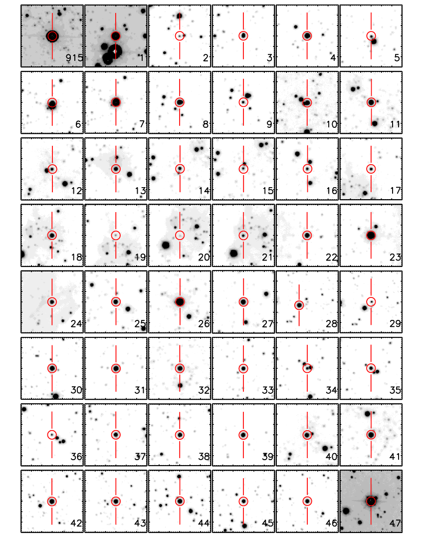
Figure 9.— UKIDSS $K$-band charts ($0\hbox to0.0pt{.\hss}^{\prime}5\times 0\hbox to0.0pt{.\hss}^{\prime}5$ ) of stars spectroscopically observed. North is up and Est to the left.

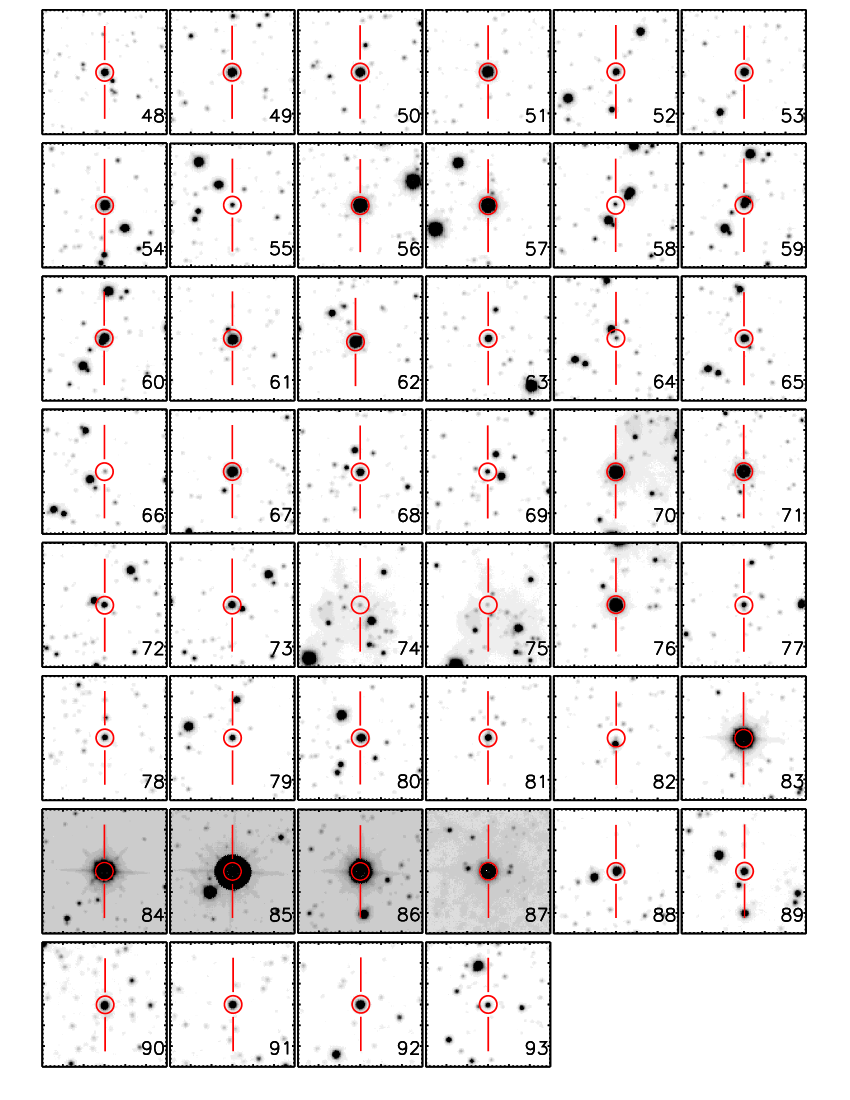
Figure 9.— Continuation of Figure 9.

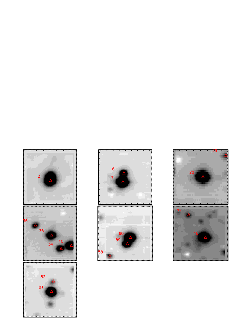
Figure 10.— Additional charts for sources not easily identifiable in Figure 9. The displayed images are obtained by averaging the SINFONI data-cubes in wavelength ($K$ grating, $8{}^{\prime\prime}\times 8{}^{\prime\prime}$).

References

- Beaumont & Williams (2010) Beaumont, C. N. & Williams, J. P. 2010, ApJ, 709, 791
- Bestenlehner et al. (2011) Bestenlehner, J. M., Vink, J. S., Gräfener, G., et al. 2011, A&A, 530, L14
- Bibby et al. (2008) Bibby, J. L., Crowther, P. A., Furness, J. P., & Clark, J. S. 2008, MNRAS, 386, L23
- Bica et al. (2003) Bica, E., Dutra, C. M., Soares, J., & Barbuy, B. 2003, A&A, 404, 223
- Bik et al. (2005) Bik, A., Kaper, L., Hanson, M. M., & Smits, M. 2005, A&A, 440, 121
- Bik et al. (2006) Bik, A., Kaper, L., & Waters, L. B. F. M. 2006, A&A, 455, 561
- Bik et al. (2010) Bik, A., Puga, E., Waters, L. B. F. M., et al. 2010, ApJ, 713, 883
- Black & van Dishoeck (1987) Black, J. H. & van Dishoeck, E. F. 1987, ApJ, 322, 412
- Blum et al. (1999) Blum, R. D., Damineli, A., & Conti, P. S. 1999, AJ, 117, 1392
- Brogan et al. (2005) Brogan, C. L., Gaensler, B. M., Gelfand, J. D., et al. 2005, ApJ, 629, L105
- Brogan et al. (2006) Brogan, C. L., Gelfand, J. D., Gaensler, B. M., Kassim, N. E., & Lazio, T. J. W. 2006, ApJ, 639, L25
- Carey et al. (2009) Carey, S. J., Noriega-Crespo, A., Mizuno, D. R., et al. 2009, PASP, 121, 76
- Chen et al. (2013) Chen, C.-H. R., Indebetouw, R., Muller, E., et al. 2013, Proc. IAU Symp. 292, ed. by T. Wong & J. Ott, Vol. 292, p. 307
- Churchwell et al. (2009) Churchwell, E., Babler, B. L., Meade, M. R., et al. 2009, PASP, 121, 213
- Churchwell et al. (2006) Churchwell, E., Povich, M. S., Allen, D., et al. 2006, ApJ, 649, 759
- Clark et al. (2011) Clark, J. S., Arkharov, A., Larionov, V., et al. 2011, Bulletin de la Societe Royale des Sciences de Liege, 80, 361
- Clark et al. (2009a) Clark, J. S., Crowther, P. A., Larionov, V. M., et al. 2009a, A&A, 507, 1555
- Clark et al. (2009b) Clark, J. S., Davies, B., Najarro, F., et al. 2009b, A&A, 504, 429
- Clark & Porter (2004) Clark, J. S. & Porter, J. M. 2004, A&A, 427, 839
- Clark et al. (2013) Clark, J. S., Ritchie, B. W., & Negueruela, I. 2013, A&A, 560, A11
- Cohen et al. (1975) Cohen, M., Kuhi, L. V., & Barlow, M. J. 1975, A&A, 40, 291
- Conti & Crowther (2004) Conti, P. S. & Crowther, P. A. 2004, MNRAS, 355, 899
- Crowther (2007) Crowther, P. A. 2007, ARA&A, 45, 177
- Crowther et al. (2006a) Crowther, P. A., Hadfield, L. J., Clark, J. S., Negueruela, I., & Vacca, W. D. 2006a, MNRAS, 372, 1407
- Crowther et al. (2006b) Crowther, P. A., Lennon, D. J., & Walborn, N. R. 2006b, A&A, 446, 279
- Dame et al. (2001) Dame, T. M., Hartmann, D., & Thaddeus, P. 2001, ApJ, 547, 792
- Davies et al. (2012) Davies, B., Clark, J. S., Trombley, C., et al. 2012, MNRAS, 419, 1871
- Davies et al. (2010) Davies, B., Lumsden, S. L., Hoare, M. G., Oudmaijer, R. D., & de Wit, W.-J. 2010, MNRAS, 402, 1504
- de Jager (1998) de Jager, C. 1998, A&A Rev., 8, 145
- DENIS Consortium (2005) DENIS Consortium. 2005, VizieR Online Data Catalog, 2263, 0
- Deharveng et al. (2010) Deharveng, L., Schuller, F., Anderson, L. D., et al. 2010, A&A, 523, A6
- Egan et al. (2003) Egan, M. P., Price, S. D., Kraemer, K. E., et al. 2003, VizieR Online Data Catalog, 5114, 0
- Eisenhauer et al. (2003) Eisenhauer, F., Abuter, R., Bickert, K., et al. 2003, Proc. Instrument Design and Performance for Optical/Infrared Ground-based Telescopes, ed. by M. Iye & A. F. M. Moorwood, SPIE Conf. Ser. 4841, p. 1548
- Ekström et al. (2012) Ekström, S., Georgy, C., Eggenberger, P., et al. 2012, A&A, 537, A146
- Eldridge et al. (2013) Eldridge, J. J., Fraser, M., Smartt, S. J., Maund, J. R., & Crockett, R. M. 2013, MNRAS, 436, 774
- Epchtein et al. (1994) Epchtein, N., de Batz, B., Copet, E., et al. 1994, Ap&SS, 217, 3
- Faherty et al. (2014) Faherty, J. K., Shara, M. M., Zurek, D., Kanarek, G., & Moffat, A. F. J. 2014, AJ, 147, 115
- Figer et al. (2002) Figer, D. F., Kim, S. S., Morris, M., et al. 2002, ApJ, 525, 750
- Figer et al. (2006) Figer, D. F., MacKenty, J. W., Robberto, M., et al. 2006, ApJ, 643, 1166
- Figer et al. (1997) Figer, D. F., McLean, I. S., & Najarro, F. 1997, ApJ, 486, 420
- Figer et al. (2002) Figer, D. F., Najarro, F., Gilmore, D., et al. 2002, ApJ, 581, 258
- Gautier et al. (1976) Gautier, III, T. N., Fink, U., Larson, H. P., & Treffers, R. R. 1976, ApJ, 207, L129
- Georgy et al. (2012) Georgy, C., Ekström, S., Meynet, G., et al. 2012, A&A, 542, A29
- Güdel & Nazé (2009) Güdel, M. & Nazé, Y. 2009, A&A Rev., 17, 309
- Hadfield et al. (2007) Hadfield, L. J., van Dyk, S. D., Morris, P. W., et al. 2007, MNRAS, 376, 248
- Halpern et al. (2012) Halpern, J. P., Gotthelf, E. V., & Camilo, F. 2012, ApJ, 753, L14
- Hanson et al. (1996) Hanson, M. M., Conti, P. S., & Rieke, M. J. 1996, ApJS, 107, 281
- Hanson et al. (2005) Hanson, M. M., Kudritzki, R.-P., Kenworthy, M. A., Puls, J., & Tokunaga, A. T. 2005, ApJS, 161, 154
- Haschick & Ho (1983) Haschick, A. D. & Ho, P. T. P. 1983, ApJ, 267, 638
- Helfand et al. (2006) Helfand, D. J., Becker, R. H., White, R. L., Fallon, A., & Tuttle, S. 2006, AJ, 131, 2525
- Helfand et al. (2007) Helfand, D. J., Gotthelf, E. V., Halpern, J. P., et al. 2007, ApJ, 665, 1297
- Humphreys & McElroy (1984) Humphreys, R. M. & McElroy, D. B. 1984, ApJ, 284, 565
- Immer et al. (2014) Immer, K., Galván-Madrid, R., König, C., Liu, H. B., & Menten, K. M. 2014, A&A, 572, 63
- Immer et al. (2013) Immer, K., Reid, M. J., Menten, K. M., Brunthaler, A., & Dame, T. M. 2013, A&A, 553, A117
- Johnson (1966) Johnson, H. L. 1966, ARA&A, 4, 193
- Kleinmann & Hall (1986) Kleinmann, S. G. & Hall, D. N. B. 1986, ApJS, 62, 501
- Koornneef (1983) Koornneef, J. 1983, A&A, 128, 84
- Kudritzki et al. (2014) Kudritzki, R.-P., Urbaneja, M. A., Bresolin, F., Hosek, Jr., M. W., & Przybilla, N. 2014, ApJ, 788, 56
- Leitherer et al. (1997) Leitherer, C., Chapman, J. M., & Koribalski, B. 1997, ApJ, 481, 898
- Lejeune & Schaerer (2001) Lejeune, T. & Schaerer, D. 2001, A&A, 366, 538
- Levesque et al. (2005) Levesque, E. M., Massey, P., Olsen, K. A. G., et al. 2005, ApJ, 628, 973
- Lockman (1989) Lockman, F. J. 1989, ApJS, 71, 469
- Lucas et al. (2008) Lucas, P. W., Hoare, M. G., Longmore, A., et al. 2008, MNRAS, 391, 136
- Ma et al. (2013) Ma, Y., Zhou, J., Esimbek, J., et al. 2013, Ap&SS, 345, 297
- Martín-Hernández et al. (2003) Martín-Hernández, N. L., van der Hulst, J. M., & Tielens, A. G. G. M. 2003, A&A, 407, 957
- Martins et al. (2007) Martins, F., Genzel, R., Hillier, D. J., et al. 2007, A&A, 468, 233
- Martins et al. (2008) Martins, F., Hillier, D. J., Paumard, T., et al. 2008, A&A, 478, 219
- Martins & Plez (2006) Martins, F. & Plez, B. 2006, A&A, 457, 637
- Martins et al. (2005) Martins, F., Schaerer, D., & Hillier, D. J. 2005, A&A, 436, 1049
- Mauerhan et al. (2011) Mauerhan, J. C., Van Dyk, S. D., & Morris, P. W. 2011, AJ, 142, 40
- McLean et al. (1998) McLean, I. S., Becklin, E. E., Bendiksen, O., et al. 1998, Proc. Infrared Astronomical Instrumentation, ed. by A. M. Fowler, SPIE Conf. Ser. 3354, p. 566
- Mercer et al. (2005) Mercer, E. P., Clemens, D. P., Meade, M. R., et al. 2005, ApJ, 635, 560
- Messineo et al. (2011) Messineo, M., Davies, B., Figer, D. F., et al. 2011, ApJ, 733, 41
- Messineo et al. (2008) Messineo, M., Figer, D. F., Davies, B., et al. 2008, ApJ, 683, L155
- Messineo et al. (2005) Messineo, M., Habing, H. J., Menten, K. M., et al. 2005, A&A, 435, 575
- Messineo et al. (2012) Messineo, M., Menten, K. M., Churchwell, E., & Habing, H. 2012, A&A, 537, A10
- Messineo et al. (2014a) Messineo, M., Menten, K. M., Figer, D. F., et al. 2014a, A&A, 569, A20
- Messineo et al. (2014b) Messineo, M., Qingfeng, Z., Ivanov, V. D., et al. 2014b, A&A, 571, 43
- Modigliani et al. (2007) Modigliani, A., Hummel, W., Abuter, R., et al. 2007, ArXiv Astrophysics arXiv:astro-ph/0701297
- Najarro et al. (1994) Najarro, F., Hillier, D. J., Kudritzki, R. P., et al. 1994, A&A, 285, 573
- Najarro et al. (1997) Najarro, F., Hillier, D. J., & Stahl, O. 1997, A&A, 326, 1117
- Negueruela et al. (2010) Negueruela, I., Clark, J. S., & Ritchie, B. W. 2010, A&A, 516, A78
- Negueruela et al. (2008) Negueruela, I., Marco, A., Herrero, A., & Clark, J. S. 2008, A&A, 487, 575
- Oh et al. (2014) Oh, S., Kroupa, P., & Banerjee, S. 2014, MNRAS, 437, 4000
- Panagia (1973) Panagia, N. 1973, AJ, 78, 929
- Pfalzner (2009) Pfalzner, S. 2009, A&A, 498, L37
- Povich et al. (2008) Povich, M. S., Benjamin, R. A., Whitney, B. A., et al. 2008, ApJ, 689, 242
- Preibisch et al. (2011) Preibisch, T., Ratzka, T., Kuderna, B., et al. 2011, A&A, 530, A34
- Price et al. (2001) Price, S. D., Egan, M. P., Carey, S. J., Mizuno, D. R., & Kuchar, T. A. 2001, AJ, 121, 2819
- Reid et al. (2009) Reid, M. J., Menten, K. M., Zheng, X. W., et al. 2009, ApJ, 700, 137
- Rubin (1968) Rubin, R. H. 1968, ApJ, 154, 391
- Sana et al. (2014) Sana, H., Le Bouquin, J.-B., Lacour, S., et al. 2014, ApJS, 215, 15
- Schreiber et al. (2004) Schreiber, J., Thatte, N., Eisenhauer, F., et al. 2004, Proc. Astronomical Data Analysis Software and Systems (ADASS) XIII, edited by F. Ochsenbein, M. G. Allen, & D. Egret, ASP Conf. Ser. 314, p. 380
- Scoville et al. (1983) Scoville, N., Kleinmann, S. G., Hall, D. N. B., & Ridgway, S. T. 1983, ApJ, 275, 201
- Shara et al. (2012) Shara, M. M., Faherty, J. K., Zurek, D., et al. 2012, AJ, 143, 149
- Shenar et al. (2014) Shenar, T., Hamann, W.-R., & Todt, H. 2014, A&A, 562, A118
- Sidorin et al. (2014) Sidorin, V., Douglas, K. A., Palouš, J., Wünsch, R., & Ehlerová, S. 2014, A&A, 565, A6
- Skrutskie et al. (2006) Skrutskie, M. F., Cutri, R. M., Stiening, R., et al. 2006, AJ, 131, 1163
- Soto et al. (2013) Soto, M., Barbá, R., Gunthardt, G., et al. 2013, A&A, 552, A101
- Stetson (1987) Stetson, P. B. 1987, PASP, 99, 191
- Storey & Hummer (1995) Storey, P. J. & Hummer, D. G. 1995, MNRAS, 272, 41
- Vacca et al. (1996) Vacca, W. D., Garmany, C. D., & Shull, J. M. 1996, ApJ, 460, 914
- van der Hucht (2001) van der Hucht, K. A. 2001, New A Rev., 45, 135
- Vollmann & Eversberg (2006) Vollmann, K. & Eversberg, T. 2006, Astronomische Nachrichten, 327, 862
- Walborn & Blades (1997) Walborn, N. R. & Blades, J. C. 1997, ApJS, 112, 457
- Watson et al. (2008) Watson, C., Povich, M. S., Churchwell, E. B., et al. 2008, ApJ, 681, 1341
- Wegner (1994) Wegner, W. 1994, MNRAS, 270, 229
- White et al. (2005) White, R. L., Becker, R. H., & Helfand, D. J. 2005, AJ, 130, 586
- Williams (1996) Williams, P. M. 1996, Proc. Radio emission from the stars and the sun, ed. by A. R. Taylor & J. M. Paredes, ASP Conf. Ser. 93, p. 15
- Wright et al. (2010) Wright, E. L., Eisenhardt, P. R. M., Mainzer, A. K., et al. 2010, AJ, 140, 1868
- Wright et al. (2014) Wright, N. J., Parker, R. J., Goodwin, S. P., & Drake, J. J. 2014, MNRAS, 438, 639
- Zacharias et al. (2004) Zacharias, N., Monet, D. G., Levine, S. E., et al. 2004, American Astronomical Society Meeting (AAS) 205. BAAS, Vol. 36, p. 1418