Biases in the determination of dynamical parameters of star clusters: today and in the Gaia era

Abstract

The structural and dynamical properties of star clusters are generally derived by means of the comparison between steady-state analytic models and the available observables. With the aim of studying the biases of this approach, we fitted different analytic models to simulated observations obtained from a suite of direct N-body simulations of star clusters in different stages of their evolution and under different levels of tidal stress to derive mass, mass function and degree of anisotropy. We find that masses can be under/over-estimated up to 50% depending on the degree of relaxation reached by the cluster, the available range of observed masses and distances of radial velocity measures from the cluster center and the strength of the tidal field. The mass function slope appears to be better constrainable and less sensitive to model inadequacies unless strongly dynamically evolved clusters and a non-optimal location of the measured luminosity function are considered. The degree and the characteristics of the anisotropy developed in the N-body simulations are not adequately reproduced by popular analytic models and can be detected only if accurate proper motions are available. We show how to reduce the uncertainties in the mass, mass-function and anisotropy estimation and provide predictions for the improvements expected when Gaia proper motions will be available in the near future.

1 Introduction

The internal kinematics of star clusters offers a wealth of information on their present day dynamical status and provides precious traces of the past history of evolution and interaction with the host galaxy of these stellar systems. In old and relatively low-mass stellar systems (like open and globular clusters) the half-mass relaxation time is often shorter that their ages and processes like kinetic energy equipartition, mass segregation and core collapse can be at work and leave signatures in the phase-space distribution of their stars. The understanding of these processes is crucial to properly model the dynamics of these stellar systems and to derive their global characteristics (total mass, mass function, degree of anisotropy, etc.) from observations performed in spatially restricted region of the cluster.

The easiest way to model the internal kinematics of star clusters is through analytic models. Alternative approaches include Jeans modelling (Ogorodnikov, Nezhinskii & Osipkov 1978; Mamon & Boué 2010), Schwarzschild’s orbit superposition method (Schwarzschild 1979; Vasiliev 2013) and comparison with Monte Carlo and N-body simulations (Giersz et al. 2008, 2009, 2011; Heggie et al. 2014). However, the former two approaches do not ensure physically meaningful solutions (i.e. the corresponding distribution function could be negative), while the latter two require an enormous computational effort and have started to become feasible for modelling rich star clusters only in recent years (e.g., see Heggie et al. 2014). Analytic models are generally defined by distribution functions depending on constants of the motion, and assume the cluster is in a steady-state and in equilibrium with the surrounding tidal field. Because star clusters are good approximation of collisions-dominated systems we have a relatively advanced understanding of the distribution of their stars in phase-space from theory and numerical simulations, and the choice of distribution function-based models is justified. The most popular model of this kind is the King (1966) model which proved to be quite effective in reproducing the surface brightness profiles of many globular clusters (GCs), open clusters and dwarf galaxies (Djorgovski 1993; McLaughlin & van der Marel 2005; Carballo-Bello et al. 2012; Miocchi et al. 2013). A generalization of this model accounting for radial anisotropy and a degree of equipartition among an arbitrary number of mass components has been provided by Gunn & Griffin (1979; see also Da Costa & Freeman 1976; Merritt 1981). The underlying assumptions of these models (i.e. the functional dependence of the distribution function on the integrals of motion and masses), although relying on a physical basis, are only arbitrary guesses to model the result of the complex interplay among many physical processes. Unfortunately, the validity of these assumptions is not easy to be tested with real data since it would require the determination of complete radial profiles, radial velocities and relative proper motions of large samples of stars with different masses. However, ground based photometric observations are not able to resolve faint low-mass stars in the cores of the most concentrated globular clusters (GCs), and Hubble Space Telescope (HST) observations are often available only for a limited portion of the cluster extent. Therefore, a single density profile is often calculated by mixing surface brightness estimates (dominated by the contribution of red giant stars) in the innermost region with main sequence (MS) star counts in the outskirts. For the same observational limits, information on the shape of the low-mass end of the mass function (MF) are available only for a few nearby GCs. Moreover, accurate line-of-sight (LOS) velocities can be derived through spectroscopic analyses only for the most massive red giant branch (RGB) stars. An even more complex task is the derivation of proper motions: to date, the typical uncertainty of the available astrometric surveys and their limiting magnitude allowed the estimate of relative proper motions only for the brightest stars of the closest GCs (McLaughlin et al. 2006; Anderson & van der Marel 2010). These data, while providing an indication of the systemic cluster motion, are not accurate enough to be used for studies on their internal dynamics. Only very recently proper motions with the right accuracy derived from extensive HST surveys are becoming available (Bellini et al. 2014; Watkins et al. 2015). In the absence of suitable observational data, Trenti & van der Marel (2013) studied the effect of two-body relaxation on the projected velocity dispersion of groups of stars with different masses in a set of N-body simulations. They noted that the simulated clusters never reach complete kinetic energy equipartition (a result already found previously by Giersz & Heggie 1997 and confirmed on real GCs by preliminary results by Bellini et al. 2013) and argued that the widely used King-Michie models could be inadequate to model these stellar systems.

Figure 1: Lagrangian radii evolution of the N-body simulation W5rh11.5R8.5 (left panel) and W5rh1R8.5 (right panel). The radii containing the 1%, 2%, 5%, 10%, 20%, 30%, 40%, 50%, 60%, 70%, 80%, 90% of the cluster mass are marked. The time at which selected snapshots are extracted are marked with dashed lines.

The possible inadequacy of these models could have serious consequences on the estimate of many intrinsic properties of GCs obtained so far. For example, since a GC is a self-gravitating system in virial equilibrium, its velocity dispersion can be used as a proxy for its mass. For this reason, many studies have been devoted in the past to the determination of dynamical masses by means of the comparison of the available photometric and kinematical observables (mainly projected density/surface brightness profiles and line-of-sight radial velocities of RGB stars) with analytic models (Mandushev, Staneva & Spasova 1991; Pryor & Meylan 1993; Lane et al. 2010; Zocchi, Bertin & Varri 2012; Kimmig et al. 2014). Because of the above mentioned lack of information on the radial distribution and kinematics of low-mass stars, these studies estimated masses through the comparison of the available data with single-mass models (such as King 1966 models) using RGB stars as tracers of the potential. This approximation, however, is incorrect and can lead to significant biases in those clusters where a large number of collisions allowed an effective exchange of kinetic energy among stars with different masses (Shanahan & Gieles 2015, hereafter SG15). Indeed, massive stars tend to transfer kinetic energy in collisions with less massive ones, becoming kinematically cold and moving on less energetic orbits at small radii. So, in these clusters both the spatial distribution and the velocity dispersion of RGB stars significantly differ from those of the other less massive stars which contribute to the largest fraction of the cluster mass. The situation is further complicated by the presence of dark remnants (white dwarfs, neutron stars and black holes) and binary stars contributing to the cluster potential but whose fraction is hard to be estimated. Because of these biases, the comparison of the derived dynamical masses with those estimated converting the cluster integrated luminosity into mass (often referred as ”luminous mass”) led to puzzling and conflicting results. Indeed, the first studies indicated that dynamical masses were $\sim$25% smaller than luminous ones (McLaughlin & van der Marel 2005; Strader et al. 2009, 2011). The above discrepancy is partly due to the adoption of RGB stars as dynamical tracers of the cluster potential, and to the neglecting of dynamical processes like the preferential losses of low-mass stars altering the mass-to-light ratio used to derive the luminous masses (Kruijssen & Mieske 2009). The above effects have been accounted for in a recent analysis by Sollima, Bellazzini & Lee (2012) who compared deep HST photometric data and an extensive survey of radial velocities for six Galactic GCs with a set of multi-mass King-Michie models, simultaneously fitting the luminosity function estimated in the innermost cluster region, the surface brightness and the velocity dispersion profile of RGB stars to derive global masses and MFs. Adopting the recipe of mass segregation of these models, they found that dynamical masses are on average $\sim$40% larger than luminous ones i.e. in the opposite direction of what found in previous analyses. In this case, while a large portion of this discrepancy can be due to an uncertain assumption of the fraction of dark remnants, a significant contribution could be due to the inadequacy of the adopted models in reproducing the degree of mass segregation of the analysed clusters.

Another aspect connected to the modelling of mass segregation of GCs regards the derivation of their global MF. Indeed, thanks to the proximity of many GCs and the high angular resolution of HST it has been possible to sample their luminosity function down to the hydrogen burning limit (Piotto, Cool & King 1997; Piotto & Zoccali 1999; Paust et al. 2010). These kind of observations are however limited to a restricted portion of the cluster, generally close to the half-mass radius (where the effects of mass segregation are minimized; Pryor, Smith & McClure 1986; Vesperini & Heggie 1997; Baumgardt & Makino 2003) or the cluster center (see e.g. the ”ACS globular clusters treasury project”; Sarajedini et al. 2007). Because of mass segregation, to derive the global MF from the local one a correction based on multi-mass modelling is necessary. This task has been performed by Paust et al. (2010) and Sollima et al. (2012) who found that the MFs of their samples of GCs can be well reproduced by power-laws with slopes varying in a wide range ($-1.7<\alpha_{MF}<-0.2$). Any possible bias in the adopted prescription for the distribution of masses would translate into a systematic error in the estimated global MF.

Finally, it is not clear if the velocity distribution of GCs stars is isotropic or if it presents some radial/tangential bias. Physical reasons at the origin of such anisotropy can be found in their mechanism of formation (possibly related to the collapse of their original gas cloud; Lynden-Bell 1967), to the collisions occurring in their central regions (Lynden-Bell & Wood 1968; Spitzer & Shull 1975) or to the interaction with the Milky Way (Oh & Lin 1992). The determination of anisotropy in GCs is extremely complex since it requires the knowledge of transverse velocities for a large sample of stars to allow an unambiguous detection, and detailed studies have been possible only very recently for the innermost regions of nearby GCs (Watkins et al. 2015). King & Anderson (2001) suggested that the dependence of the degree of anisotropy on mass could be different from what is predicted by King-Michie models.

The advent of the Global Astrometric Interferometer for Astrophysics (Gaia) will change the picture by providing accurate distances and proper motions for hundreds of stars in a large sample of nearby GCs (Pancino, Bellazzini & Marinoni 2013). Indeed, the unprecedented astrometric accuracy of Gaia will provide proper motions with an accuracy comparable to that of LOS radial velocities obtainable through high resolution spectroscopy. These measures, complemented by those soon available from the HST analyses in the central regions of GCs, could open the way for a new golden age for studies on the internal dynamics of GCs.

In this paper we will compare the most widely used analytic models with a suite of N-body simulations applying the most widely used technique to determine mass, MF and anisotropy with the aim of studying the biases in the determination of these quantities linked to the ability of analytic models to reproduce the correct phase-space structure of the simulated stellar systems. In Sect. 2 the adopted analytic models and the performed N-body simulations are described. In Sect. 3 we describe the method adopted to derive the best-fit masses and MFs. In Sect. 4 the results of the comparison between the true and the estimated masses and MFs are presented. Sect. 5 is devoted to the simulation of Gaia observations of GCs including realistic errors and radial sampling efficiency to test the feasibility of studies on GCs anisotropy. We finally summarize our results in Sect. 6

2 Simulations and Models

2.1 N-body simulations

The N-body simulations considered here have been performed using the collisional N-body codes NBODY4 and NBODY6 (Aarseth 1999) and are part of the surveys presented by Baumgardt & Makino (2003) and Lamers, Baumgardt & Gieles (2013). Each simulation contains 131072 particles with no primordial binaries, although a small number of binaries and triples form through tidal capture during the cluster evolution. In this configuration, the total cluster mass is 71236.4 $M_{\odot}$. Particles were initially distributed following a King (1966) model with central dimensionless potential $W_{0}=5$, regardless of their masses. Two simulations with different half-mass radii have been run (with $r_{h}=1$ and 11.5 pc, hereafter referred to as W5rh1R8.5 and W5rh11.5R8.5, respectively). Particle masses taken from a Kroupa (2001) MF with a lower mass limits of 0.1 $M_{\odot}$ and an upper mass limit of 15 and 100 $M_{\odot}$, for the W5rh11.5R8.5 and W5rh1R8.5 simulation respectively. The cluster moves within a logarithmic potential having circular velocity $v_{circ}=220~{}km/s$, on a circular orbit at a distance of 8.5 kpc from the galactic center. The corresponding initial Jacobi radius is $r_{J}=61.15$ pc, i.e. equal to the one of the W5rh11.5R8.5 simulation. Because of their different Roche lobe filling factors, the tidal field affects the two simulations in extremely different ways. Moreover, the initial half-mass relaxation time is significantly longer in model W5rh11.5R8.5 ($t_{rh}=4.97$ Gyr) with respect to model W5rh1R8.5 ($t_{rh}=0.12$ Gyr). So, while the mass of the considered simulations are significantly smaller than those of real GCs, they bracket the majority of globular clusters in terms of both their half-mass relaxation time and relative strength of the tidal field ($r_{J}/r_{h}$). Stellar evolution has been modeled using the fitting formula of Hurley, Pols & Tout (2000) assuming a metallicity Z=0.001. Mass lost during stellar evolution is assumed to be immediately lost from the cluster. No kick velocity has been added to stellar remnants at their birth. A certain retention fraction of newly formed black holes and neutron stars has been assumed: in simulation W5rh11.5R8.5 no black holes are present and all neutron stars are assumed to be retained at their birth, while in simulation W5rh1R8.5 we assumed that 10% neutron stars and black holes are retained. The temperature and luminosity of each star is recorded at each time-step according to its evolutionary stage. Simulations have been run until cluster dissolution, defined to be the time when 95% of the initial mass has been lost. The evolution of the Lagrangian radii of the two simulations is shown in Fig. 1. After the initial expansion driven by stellar evolution mass-loss, simulation W5rh1R8.5 quickly undergoes core-collapse (after $\sim$5 Gyr), and continues its evolution expanding slowly. Instead, because of its longer relaxation time, simulation W5rh11.5R8.5 follows a slow evolution losing a large fraction of its stars because of the strong tidal field.

2.2 Analytic models

Selected snapshots of the above N-body simulations have been extracted and their projected properties (density and LOS velocity dispersion profiles) have been compared with a set of King-Michie models (Gunn & Griffin 1979). These models are constructed from a lowered-Maxwellian distribution function made by the contributions of H mass groups

$$f(E,L) = \sum_{i=1}^{H}k_{i}exp\left(-\frac{A_{i}L^{2}}{2\sigma_{K}^{2}r_{a}^{2}}\right)\left[exp\left(-\frac{A_{i}E}{\sigma_{K}^{2}}\right)-1\right]$$

$$\sum_{i=1}^{H}f_{i}(r,v_{r},v_{t}) = \sum_{i=1}^{H}k_{i}exp\left[-A_{i}\frac{v_{t}^{2}}{2\sigma_{K}^{2}}\left(\frac{r}{r_{a}}\right)^{2}\right]\times$$

$$\left[exp\left(-\frac{A_{i}(v_{r}^{2}+v_{t}^{2}+2\psi)}{2\sigma_{K}^{2}}\right)-1\right]$$

where $E$ and $L$ are, respectively, the energy and angular momentum per unit mass, $v_{r}$ and $v_{t}$ are the radial and tangential components of the velocity, the effective potential $\psi$ is the difference between the cluster potential $\phi$ at a given radius $r$ and the potential at the cluster tidal radius $\psi\equiv\phi-\phi_{t}$, $A_{i}$ and $k_{i}$ are scale factors for each mass group, and $\sigma_{K}$ is a normalization term. Note that the above distribution function allows for various levels of radial anisotropy but does not allow tangential anisotropy. The number density and the radial and tangential components of the velocity dispersion of each mass group are obtained by integrating Eq. 2.2:

$$n_{i}(r) = 4\pi\int_{0}^{\sqrt{-2\psi}}\int_{0}^{\sqrt{-2\psi-v_{r}^{2}}}v_{t}f_{i}(r,v_{r},v_{t})dv_{t}dv_{r},$$

$$\sigma_{r,i}^{2}(r) = \frac{4\pi}{m_{i}n_{i}(r)}\int_{0}^{\sqrt{-2\psi}}v_{r}^{2}\int_{0}^{\sqrt{-2\psi-v_{r}^{2}}}v_{t}f_{i}(r,v_{r},v_{t})dv_{t}dv_{r},$$

$$\sigma_{t,i}^{2}(r) = \frac{4\pi}{m_{i}n_{i}(r)}\int_{0}^{\sqrt{-2\psi}}\int_{0}^{\sqrt{-2\psi-v_{r}^{2}}}v_{t}^{3}f_{i}(r,v_{r},v_{t})dv_{t}dv_{r}$$

Equations 2.2 can be written in terms of dimensionless quantities by substituting

$$\zeta = \frac{v_{r}^{2}}{2\sigma_{K}^{2}},\eta=\frac{v_{t}^{2}}{2\sigma_{K}^{2}},$$

$$\tilde{\rho}_{i} = \frac{m_{i}n_{i}}{\sum_{j}m_{j}n_{0,j}},\tilde{r}=\frac{r}{r_{c}},$$

$$W = -\frac{\psi}{\sigma_{K}^{2}},\tilde{r}_{a}=\frac{r_{a}}{r_{c}},$$

where $\rho_{0}=\sum_{j}m_{j}n_{0,j}$ is the central cluster density and

$$r_{c}\equiv\left(\frac{9\sigma_{K}^{2}}{4\pi G\rho_{0}}\right)^{1/2}$$

is the core radius (King 1966). The potential at each radius is determined by the Poisson equation

$$\nabla^{2}\psi=4\pi G\rho$$ (3)

Equations 2.2 and 3 have been integrated after assuming as a boundary condition a value of the dimensionless potential at the center $W_{0}$ outward till the radius $r_{t}$ at which both density and potential vanish. The total mass of the cluster $M$ is then given by the sum of the masses of all the groups

$$M = \sum_{i=1}^{H}m_{i}N_{i}$$

$$= \frac{9r_{c}\sigma_{K}^{2}}{G}\sum_{i=1}^{H}\int_{0}^{r_{t}}\tilde{\rho}_{i}\tilde{r}^{2}d\tilde{r}$$

As a last step, the above profiles have been projected onto the plane of the sky to obtain the surface density

$$\Sigma_{i}(R)=2\int_{R}^{r_{t}}\frac{n_{i}r}{\sqrt{r^{2}-R^{2}}}dr$$

the velocity dispersion along the line-of-sight, and in the projected radial and tangential directions in the plane of the sky

$$\sigma_{LOS,i}^{2}(R) = \frac{1}{\Sigma_{i}}\int_{R}^{r_{t}}\frac{n_{i}[2\sigma_{r,i}^{2}(r^{2}-R^{2})+\sigma_{t,i}^{2}R^{2}]}{r\sqrt{r^{2}-R^{2}}}dr$$

$$\sigma_{r^{\prime},i}^{2}(R) = \frac{1}{\Sigma_{i}}\int_{R}^{r_{t}}\frac{n_{i}[2\sigma_{r,i}^{2}R^{2}+\sigma_{t,i}^{2}(r^{2}-R^{2})]}{r\sqrt{r^{2}-R^{2}}}dr$$

$$\sigma_{t^{\prime},i}^{2}(R) = \frac{1}{\Sigma_{i}}\int_{R}^{r_{t}}\frac{n_{i}\sigma_{t,i}^{2}r}{\sqrt{r^{2}-R^{2}}}dr$$

The MF of unevolved stars in an annulus defined at a given distance R and with a width $\Delta R$ is given by

$$N_{i}(R,\Delta R)=2\pi\mu_{i}\int_{R-\Delta R/2}^{R+\Delta R/2}R~{}\Sigma_{i}dR$$ (5)

while the cumulative distribution of a sample of k bins from j to j+k

$$N(<R)=2\pi\sum_{i=j}^{j+k}\mu_{i}\int_{0}^{R}R~{}\Sigma_{i}dR$$ (6)

where $\mu_{i}=1-N_{i}^{remn}/N_{i}$ is the fraction of unevolved stars and $N_{i}^{remn}$ is the number of remnants in the i-th mass bin.

In the above models, for any choice of the $A_{i}$ coefficients, the shape of the density and velocity dispersion profiles are completely determined by the parameters ($W_{0},\tilde{r}_{a},N_{i}$) while their normalization is set by the pair of parameters ($r_{c},M$).

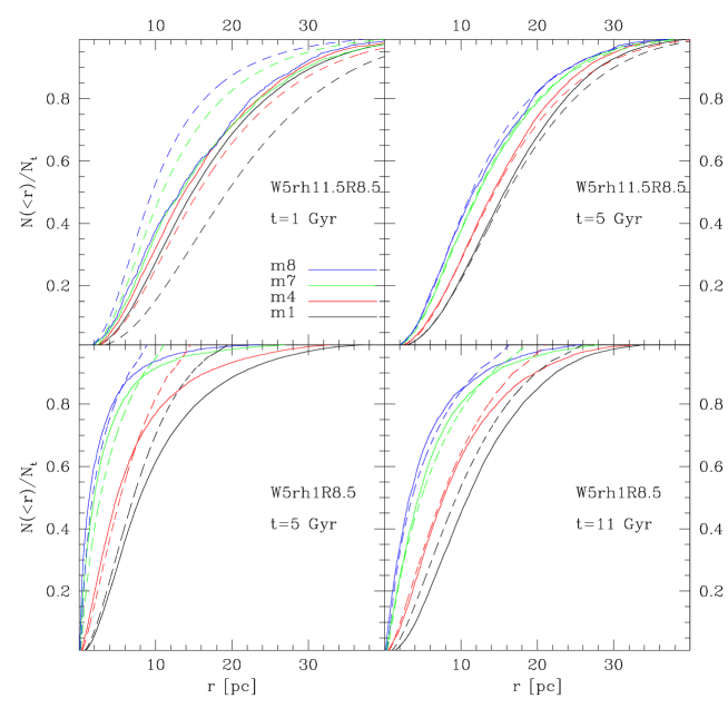
Figure 2: Cumultive radial distribution of different mass groups in the selected snapshots of the performed N-body simulations (solid lines). The prediction of the best-fit King-Michie model (assuming $\alpha=1$) are marked with dashed lines.

The dependence on mass of the coefficients $A_{i}$ determines the degree of mass segregation of the cluster. In the formulation by Gunn & Griffin (1979) $A_{i}\propto m_{i}$ which implies that more massive stars are kinematically colder than less massive ones. Note however that, according to Eq. 2.2 and assuming isotropy, the actual squared velocity dispersion of the i-th mass group is

$$\sigma_{i}^{2}=\frac{6\sigma_{K}^{2}}{5A_{i}}\frac{\gamma(7/2,A_{i}W)}{\gamma(5/2,A_{i}W)}$$

where $\gamma(a,b)\equiv\int_{0}^{b}x^{a-1}e^{-x}dx$ is the lower incomplete gamma function. According to the above equation, if $A_{i}\propto m_{i}$ complete equipartition is achieved only in the limit $W\rightarrow+\infty$. So, these models do not assume kinetic energy equipartition neither locally nor globally (see also Merritt 1981). A slight modification to the Gunn & Griffin (1979) assumption can be made to allow intermediate levels of relaxation, by simply assuming $A_{i}\propto m_{i}^{\alpha}$. In this case $\alpha=0$ models correspond to single-mass King (1966) models, $\alpha=1$ to Gunn & Griffin (1979) models. We note that for $\alpha\rightarrow+\infty$ the distribution function of low-mass stars tends asymptotically to $f(E)\propto-A_{i}E/2\sigma_{K}$ i.e. there is a maximum degree of kinetic energy equipartition reachable by these models. Moreover, extrapolation at values of $\alpha>>1$ produces unrealistic density and velocity dispersion profiles.

3 method

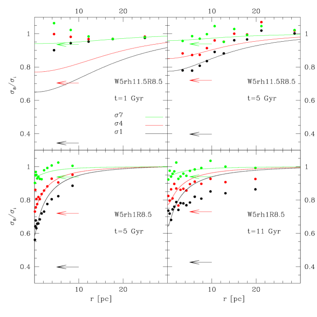
Figure 3: Ratio between the velocity dispersion of the most massive and those of less massive bins as a function of distance from the cluster center for the selected snapshots of the performed N-body simulations. The prediction of the best-fit King-Michie models (assuming $\alpha=1$) are shown with solid lines. The values corresponding to kinetic energy equipartition are marked with arrows.

The aim of this paper is to check the ability of analytic models to reproduce the main kinematical properties of simulated star clusters. For this purpose, we used selected snapshots of the simulations described in Sect. 2.1 to produce mock observations, by considering only those information generally available to observers. In particular, for each analysed snapshot we extracted:

• the projected number density profile of the brightest stars;

• the MF of unevolved stars ($N_{i}^{obs}(R_{d})$) estimated in a 1 pc-width annulus around a given distance from the cluster center (hereafter referred as the deep field range);

• the LOS velocities of the brightest stars.

Projected distances and velocities have been calculated by projecting 3D positions and velocities along a random direction. We considered only stars whose projected distance lies within the Jacobi radius, to avoid the inclusion of tidal tails in our sample. As described in Sect. 2.2, analytic models are constructed from the superposition of different mass bins. Here we considered 8 evenly spaced mass bins ranging from 0.1 $M_{\odot}$ to the mass at the RGB tip ($M_{tip}$), plus an additional bin containing all the remnants more massive than $M_{tip}$. The particles of the simulation have been divided in the above defined mass bins according to their masses. As we are interested in systematic biases (and not in random uncertainties) we have not added observational errors and incompleteness effects to our data. Moreover, we assumed that the fraction ($\mu_{i}$) and the mass distribution of dark remnants ($N_{i}^{remn}$) are known a priori by the observer. This last assumption is far from reality and in real cases this uncertainty can even represent the largest source of systematics (see Sollima et al. 2012). However, as our purpose is to determine the impact of the adopted criterion for relaxation we neglect this issue. The impact of the uncertainties on dark remnants will be addressed in a forthcoming paper (Peuten et al., in preparation).

The best fit to the above defined quantities has been performed using a Markov-Chain Monte Carlo (MCMC) algorithm nested into an iterative procedure (see Sollima et al. 2012). We performed the following steps:

1. We adopted as a first guess of the global MF ($N_{i}$) the sum of the local MF of unevolved stars measured in the deep field range ($N_{i}^{obs}$) and that of remnants ($N_{i}^{remn}$);

2. the MCMC algorithm samples the parameter space to find the pair of parameters ($W_{0},~{}r_{c}$) minimizing the Kolmogorov-Smirnov penalty function i.e. the maximum absolute difference between the observed and the predicted normalized cumulative distribution of particles in the considered mass bins (excluding remnants; see Eq. 6). The probability associated to the Kolmogorov-Smirnov test $P_{KS}$ is recorded;

3. The MF predicted by the model in the deep field range ($N_{i}^{mod}$) is calculated using Eq. 5 and a new guess ($N^{\prime}_{i}$) of the global MF of unevolved stars is made using the relation

   $$N^{\prime}_{i}=N_{i}\left(\frac{N_{i}^{obs}}{N_{i}^{mod}}\right)^{0.5}$$

   where the exponent 0.5 is a damping factor to avoid divergence.

Steps (ii) and (iii) are repeated until the maximum variation of the estimated MF in two subsequent iterations among the various mass bins ($max|1-N^{\prime}_{i}/N_{i}|$) falls below 1%.

The mass of the model has been finally derived by minimizing the log-likelihood function

$$lnL=lnP_{KS}-\frac{1}{2}\sum_{i=1}^{N}\frac{(v_{i}-\bar{v})^{2}}{\sigma_{LOS}^{2}(R_{i})}+ln(\sigma_{LOS}(R_{i}))$$ (7)

Where $v_{i}$ is the LOS radial velocity of the i-th star belonging to the most massive group. An additional cycle can be added to the above procedure to search for the value of the anisotropy radius $\tilde{r}_{a}$ maximizing the above defined merit function.

4 Results

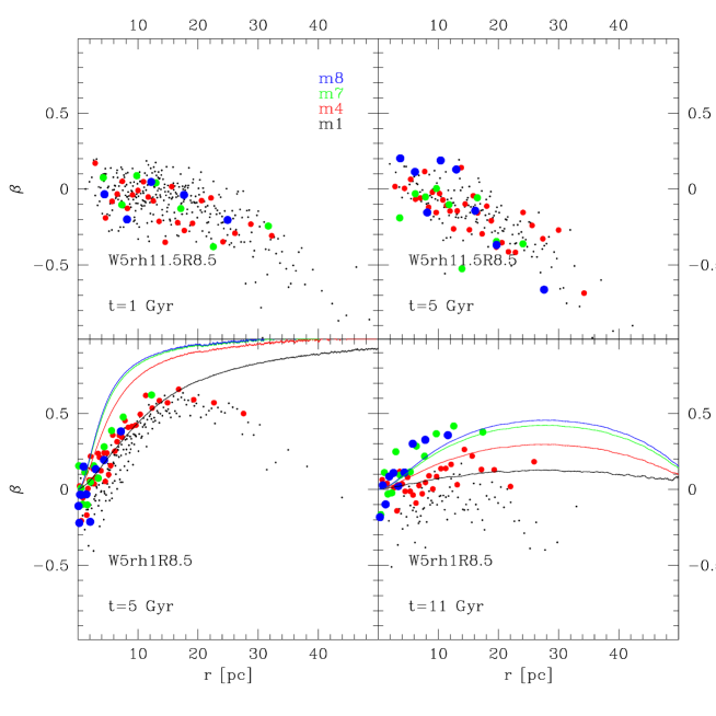
Figure 4: Anisotropy parameter as a function of the distance from the cluster center for various mass groups in the selected snapshots of the performed N-body simulations. The prediction of the best-fit King-Michie models (assuming $\alpha=1$) are marked with solid lines.

As a first test we selected two snapshots for each simulation in selected moments of the cluster evolution and compared the radial distribution, velocity dispersion and anisotropy of different mass groups with those predicted by the corresponding best-fit models. In particular, for the less evolved simulation W5rh11.5R8.5 we selected a snapshot at 1 Gyr (after the stellar evolution-driven expansion and before a significant level of relaxation has been reached) and a snapshot at 5 Gyr ($t\sim 0.8~{}t_{rh}(t)$). For simulation W5rh1R8.5 snapshots at 5 Gyr (close to core collapse) and 11 Gyr (after several half-mass relaxation times; $t\sim 9t_{rh}(t)$) have been selected.

In Fig. 2 the cumulative radial distribution of four different mass groups are compared with those predicted by the best-fit King-Michie models assuming $\alpha$=1. As expected, in the early stage of evolution of simulation W5rh11.5R8.5 different mass groups have still very similar distributions. In this case, the best-fit multi-mass model overpredicts the level of relaxation predicting low-mass stars distributed on a more extended structure than they really are. On the other hand, after 5 Gyr the cluster reaches the level of relaxation adopted by the model, which reproduces extremely well the radial distribution of all the mass groups. A different situation occurs in simulation W5rh1R8.5: in both the selected stages of evolution the actual mass segregation is slightly larger than that predicted by King-Michie models.

The same conclusion can be reached by analysing the ratio between the 3D velocity dispersions of different mass bins (see Fig. 3). In a relaxed stellar system kinetic energy equipartition implies that at each radius the velocity dispersion of stars scales with their masses as $\sigma\propto m^{-1/2}$. So, while at the beginning of the simulation stars of different masses have the same dispersion, as relaxation proceeds massive stars tend to became kinematically colder than less massive ones and the ratio of their velocity dispersions tends to the square root of their mass ratios. This process is faster in the center of the cluster where a large number of collisions accelerates this process. An inspection of Fig. 3 shows that, as already mentioned in Sect. 2.2, both N-body simulations and analytic models are still far from complete kinetic energy equipartition even in the cluster center. Again, models overpredict relaxation in the first selected snapshot of simulation W5rh11.5R8.5 while they well reproduce the velocity dispersion ratio in all the other considered snapshots of both simulations, except for the least massive bin which appears over-relaxed in simulation W5rh1R8.5 than what predicted by analytical models.

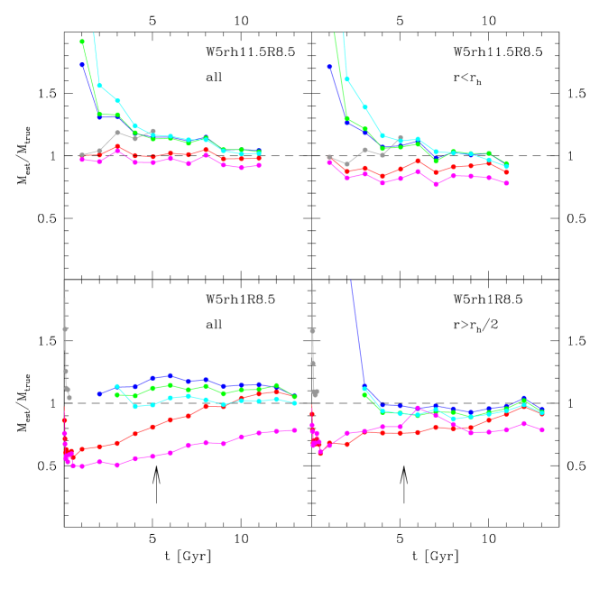
Figure 5: Ratio between the masses estimated by analytic models and the true cluster mass. The color code of different models in described in Sect. 4. Left panels refer to mass estimates performed using the entire sample of giants, right panels refer to estimates performed applying a radial selection to the sample. The epoch of core-collapse in simulation W5rh1R8.5 is marked by an arrow in bottom panels.

In Fig. 4 the anisotropy parameter $\beta\equiv 1-\sigma^{2}_{t}/2\sigma^{2}_{r}$ of the various mass groups is shown as a function of the distance from the cluster center. A positive value of $\beta$ indicates a bias toward radial orbits (radial anisotropy), while a negative value indicates the prevalence of tangential orbits (tangential anisotropy). It is apparent that the two simulations present opposite trends: in both the considered snapshots of simulation W5rh11.5R8.5 tangential anisotropy which increases toward the outer cluster regions is apparent in all mass bins with the same indistinguishable amplitude. Instead, in simulation W5rh1R8.5 all mass groups quickly develop radial anisotropy. After many relaxation times, however, this trend tends to be erased in the less-massive stars whose orbits became again isotropic, while a significant radial anisotropy persists in the most massive stars. The physical reason of this behaviour is likely due to the different tidal stress experienced by the two simulations: in simulation W5rh1R8.5 collisions occurring in the cluster center kick stars in the cluster halo on radial orbits. This process, already studied in past studies by Lynden-Bell & Wood 1968 and Spitzer & Shull 1975, appears to affect stars of different masses with the same efficiency. In the initial stage of this simulation the cluster is very compact and almost unaffected by the tidal field. As evolution proceeds, the cluster expands and the kinematically hottest low-mass stars reach the boundary of the Roche volume. In this case, stars on radial orbits reach this boundary with positive velocity and escape more efficiently from the cluster. This process produces the observed increasing trend of radial anisotropy with mass. The same effect is at work during the entire evolution of simulation W5rh11.5R8.5: in this case, the cluster feels a strong tidal field and stars on tangential orbits are preferentially retained regardless of their masses. The comparison with King-Michie models has been done only for the snapshots of the W5rh1R8.5 simulation. Indeed, these models do not account for tangential anisotropy present in the W5rh11.5R8.5 simulation. It is apparent that King-Michie models predict an increasing anisotropy for more massive stars. So, while they reproduce fairly well the snapshot at 11 Gyr, they cannot provide a satisfactory representation of the cluster in its early stages.

Summarizing, King-Michie models with $\alpha=1$ (i.e. $A_{i}\propto m_{i}$ as in the formulation by Gunn & Griffin 1979) appear to qualitatively reproduce the radial distribution and relaxation status of the performed N-body simulations after a timescale comparable to the half-mass relaxation time. On the other hand, the formalism of these models does not allow to reproduce the general characteristics of the velocity anisotropy in all the stages of evolution of the simulated clusters.

To quantify the ability of these models to reproduce the estimated mass and MFs we fitted models to a large number of snapshots of the two considered simulations under different assumptions on the available range of stars used to compute the density profile and the location of the deep field used to estimate the local MF. In particular, we considered the following fits:

1. single-mass King (1966) models ($\alpha=0$) fitting the number density profile constructed with the 4 most massive bins (red lines in Fig.s 5 and 7);

2. single-mass King (1966) models ($\alpha=0$) fitting the number density profile constructed with only the most massive bin (magenta lines);

3. multi-mass King-Michie models ($\alpha=1$) fitting the number density profile constructed with the 4 most massive bins and adopting a deep field range centered around the projected half-mass radius (blue lines);

4. multi-mass King-Michie models ($\alpha=1$) fitting the number density profile constructed with only the most massive bin and adopting a deep field range centered around the projected half-mass radius (cyan lines);

5. multi-mass King-Michie models ($\alpha=1$) fitting the number density profile constructed with the 4 most massive bins and adopting a deep field range centered in the cluster center (green lines);

6. multi-mass King-Michie models fitting the number density profile constructed with the 4 most massive bins and a value of $\alpha$ chosen to simultaneously reproduce the MF measured in two deep field ranges centered at the projected half-mass radius and in the cluster center, respectively (grey lines).

Only isotropic models have been considered since i) as shown above, King-Michie models do not reproduce the qualitative trend of anisotropy with mass, ii) they do not include a treatment for tangential anisotropy occurring in some stage of evolution, and iii) in absence of proper motion information the signal of radial anisotropy (characterized by an increase of the central LOS velocity dispersion) can be mimicked by the presence of massive objects not (properly) accounted in the model (e.g. a large number of neutron stars, binaries, a sub-system of stellar mass black holes or an intermediate-mass black hole, etc.). The results of the above test are described in the next subsections.

4.1 Mass estimate

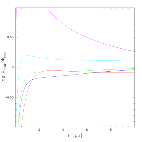
Figure 6: Ratio between the potential estimated by different models and the true potential of the snapshot at 11 Gyr of simulation W5rh1R8.5. The color codes of different models are described in Sect. 4.

In Fig. 5 the ratio between the mass estimated by the best-fit analytic models and the true mass of the simulation is plotted as a function of the cluster age. By analysing simulation W5rh1R8.5 it appears that, after the first snapshot of the simulation, single-mass models systematically underestimate the cluster mass up to 50% and improve their estimates at the end of the simulation. This is due to the quick relaxation reached by this simulation after few Myr: as already explained in Sect. 1, in single-mass models all stars have a single kinetic temperature. When a significant level of relaxation is established massive stars (used to sample both the number density and the velocity dispersion of the cluster) have a smaller velocity dispersion with respect to other cluster stars, mimicking the behaviour of stars in the potential of a less massive cluster. Such an effect is less evident when many mass bins are used to derive the number density profile, since in this last case the derived mass distribution (and consequently the gravitational potential) is more similar to the true one. In the advanced stages of evolution the masses estimated by single-mass models increase and exceed the real value at $t>$10 Gyr. This trend occurs because of the flattening of the mass function due to the preferential escape of low-mass stars: in this stage the mean mass of stars increases and becoming more similar to that of the stars used as tracers of the cluster potential (see also SG15). Regarding multi-mass models with $\alpha=1$ they provide a better estimate of the mass after $\sim$2 Gyr, although they generally overestimate the cluster mass by 10-20%. A counterintuitive evidence is that models whose density profile is calculated only from the most massive bin perform slightly better than those where more bins have been considered. To understand the reason of such an occurrence we plot in Fig. 6 the ratio between the potential estimated by the various models and the true one in the snapshot at 11 Gyr. It is apparent that while all models generally reproduce the potential at large distances from the cluster center, the central potential is always missed by models. This region is indeed particularly difficult to be reproduced because massive remnants or binaries can sink into the very central part of the cluster producing a cusp-like shape not reproduced by models. We repeated the mass estimate by excluding the innermost region at $r<r_{h}/2$. In this last case multi-mass models adequately reproduce the cluster mass during the entire evolution (within 10% except in the initial stages) regardless of the adopted range of masses used to compute the density profile.

A different situation can be noted by analysing simulation W5rh11.5R8.5: here single-mass models always well reproduce the cluster mass, while multi-mass ones tend to overpredict the cluster mass by $\sim 10\%$. Before 2 Gyr instead, multi-mass models assuming $\alpha=1$ significantly overestimate (by more than 50%) the mass. This is because in these early stages of evolution of this simulation the cluster is still dynamically young and the low velocity dispersion of massive stars predicted by models is compensated by an increased estimated mass. The behaviour at $t>$5 Gyr is instead linked to the heating produced by the tidal field. Indeed, because of the strong tidal field experienced by the cluster in this simulation, many stars reach an energy level comparable to the potential at the tidal radius, but they take some dynamical time to escape (Fukushige & Heggie 2000; Baumgardt 2001). During this phase they remain trapped within the cluster on energetic orbits at large radii with an increased velocity dispersion. In fact, by excluding the outermost region of the cluster (at $r>r_{h}$ where the orbits of these stars are preferentially confined) the estimated masses decrease and bring back the estimates of multi-mass models on the right value. It is worth noting that the best estimate is obtained constraining the value of $\alpha$ with two measures of the MF at different distances from the cluster center.

4.2 Mass Function estimate

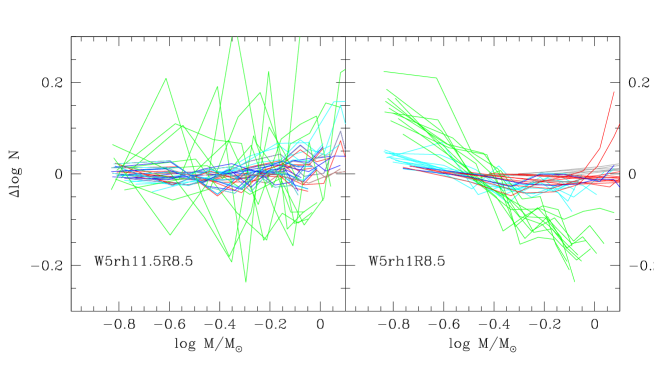
Figure 7: Difference between the actual global MFs and those estimated using various assumptions for the location of the deep field range and the mass range of stars used to compute the density profile for the two considered simulations. The color code is described in Sect. 4. Red lines in both panels indicate the differences with respect to the MF observed at the half-mass radius without applying any correction.

In Fig. 7 the differences between the true and the estimated global MFs are shown for various assumptions and snapshots of the two considered simulations. Of course, only multi-mass models have been considered in this case. It is apparent that the various assumptions on the number of bins used to construct the density profile and the choice of the correct value of $\alpha$ do not produce significant differences in the determination of the MF, providing during all the evolution a good estimate of the MF slope (within $\Delta\alpha_{MF}<0.05$). A systematic trend is instead visible in simulation W5rh1R8.5 when the global MF is measured by correcting that estimated in the cluster center: in this case a slope shallower by $\Delta\alpha_{MF}\sim 0.4$ is estimated. This is a consequence of the insufficient level of relaxation of multi-mass models which is particularly evident in the cluster center (see Sect. 4.1). Consequently, the lack of low-mass stars caused by mass segregation is erroneously interpreted as a real deficiency of stars and therefore lead to an underestimate of the MF slope. This bias is instead not visible in simulation W5rh11.5R8.5 (where this last approach is anyway the most uncertain) because in this simulation multi-mass models better reproduce the relaxation of the system. The difference between the actual global MF and that measured at the half-mass radius (without applying any correction) is also plotted in Fig. 7 for comparison. It is apparent that also in this case, no significant differences are noticeable.

5 Simulation of Gaia observations

In the previous sections we estimated the masses and the MFs of simulated clusters through the comparison with steady-state analytic models using as mass tracer the LOS velocity dispersion of the most massive cluster stars. In general, good estimates can be obtained with the desired level of accuracy provided that radial velocities for a large enough number of stars are available. The use of proper motions can improve the accuracy of the above estimates increasing the number of velocities used to constrain the cluster mass. However, the invaluable improvement provided by proper motions resides in the possibility of i) testing the level of relaxation by measuring the velocity dispersion of stars with different masses, and ii) measuring the characteristics of anisotropy. For the first task it is necessary to measure proper motions for MS stars down to a few magnitudes below the turn-off point. The faint limiting magnitude and the high angular resolution needed for this task can be achieved only with HST and will be soon available (see Bellini et al. 2014). The second task can be instead obtained even using proper motions for only the brightest massive stars. Gaia will provide proper motions for stars brighter than $g<20$ over the full sky, sampling also the RGB stars of a number of nearby GCs. An, Evans & Deason (2012) showed that the proper motions provided by Gaia will allow an accurate estimate of masses in GCs up to distances of $\sim$20 kpc. In this section we want to test if a level of anisotropy like the one developed by the simulations presented here can be detected with the accuracy of Gaia data.

In principle, we could use for this test the snapshots of the performed N-body simulations. However, the simulations considered here have masses $\sim$10 times smaller than a typical GCs, so the velocity dispersions would be significantly smaller and the crowding conditions would be less severe than in a real GC. For this reason we simulated a set mock clusters from the potential and the phase-space distribution of the best-fit anisotropic multi-mass King-Michie model of the snapshot at 11 Gyr of the simulation W5rh1R8.5, but assuming cluster masses between $4.5<log(M/M_{\odot})<6$. Positions and velocities have been projected and transformed in angular distances and proper motions assuming various heliocentric distances. Gaia magnitudes have been calculated by interpolating the particle masses through an isochrone by Marigo et al. (2008) with suitable age and metallicity. A reddening of $E(B-V)=0.1$ and the extinction coefficients by Chen et al. (2014) have been assumed. Errors on proper motions have been added using the software PyGaia provided by the Gaia Project Scientist Support team as a function of magnitude, color and assuming a K spectral type (suitable for RGB stars). These information are computed as all sky average, neglecting efficiency variations on the sky, and assuming the after-launch throughputs and error curves. Because of the angular size of the readout window, proper motions can be computed only for relatively isolated stars. Here we consider only stars with no neighbors brighter than 2.5 magnitudes with respect to the target g magnitude within $3.54\arcsec$ (see Pancino et al. 2013). Gaia will also provide radial velocities from low-resolution spectra. However, the estimated velocity errors and the limiting magnitudes are of lower quality with respect to those of available spectrographs mounted on 8m-class telescopes, so we considered errors of 0.5 km/s on radial velocities only for stars brighter than $g<17$ assuming they come from a different source.

The anisotropy parameter $\beta$ is a function of the ratio between the tangential and the radial components of the 3D velocity dispersion ($\sigma_{r}^{2}$ and $\sigma_{t}^{2}$, respectively). These quantities are related to the velocities along the LOS ($v_{LOS}$) and projected on the plane of the sky ($v_{\alpha cos\delta}$ and $v_{\delta}$) by Eq. 2.2 where

$$x = (\alpha-\alpha_{0})~{}cos\delta$$

$$y = \delta-\delta_{0}$$

$$R = \sqrt{x^{2}+y^{2}}$$

$$r = \sqrt{x^{2}+y^{2}+z^{2}}$$

$$v_{r^{\prime}} = \frac{xv_{\alpha cos\delta}+yv_{\delta}}{R}$$

$$v_{t^{\prime}} = \frac{yv_{\alpha cos\delta}-xv_{\delta}}{R}$$

$\alpha_{0}$ and $\delta_{0}$ are the right ascension and declination of the cluster center and $z$ is the distance along the LOS from the plane passing through the cluster center. As the distance along the LOS is unknown it is not possible to determine $\beta$ directly from observations. On the other hand, it is possible to combine Eq.s 2.2 to obtain

$$\beta^{\prime}(R) = \frac{\int_{R}^{r_{t}}\frac{n(r)\sigma_{r}^{2}\beta r}{\sqrt{r^{2}-R^{2}}}dr}{\int_{R}^{r_{t}}\frac{n(r)\sigma_{r}^{2}r}{\sqrt{r^{2}-R^{2}}}dr}$$

$$= 1-\frac{\sigma_{t^{\prime}}^{2}}{\sigma_{r^{\prime}}^{2}+\sigma_{LOS}^{2}-\sigma_{t^{\prime}}^{2}}$$

Since the maximum density and radial velocity dispersion in the above equation occurs at $(r=R,z=0)$, the above quantity is close to $\beta(R)$.

One thousand synthetic observations have been simulated for each choice of the cluster mass and distance and the mean value of $\langle\beta^{\prime}\rangle$ and its standard deviation $\sigma_{\beta^{\prime}}$ have been calculated for those stars with both radial velocities and proper motions estimates. The $\beta^{\prime}$ value of each synthetic observation has been calculated using the maximum-likelihood algorithm described by Eq. 7 to calculate $\sigma_{LOS},~{}\sigma_{r^{\prime}}$ and $\sigma_{t^{\prime}}$ where individual errors on velocities ($\epsilon_{i}$) have been added to the intrinsic velocity dispersion ($\sigma_{intr}$) assuming $\sigma_{i}^{2}=\sigma_{intr}^{2}+\epsilon_{i}^{2}$. The significance level (defined as $\langle\beta^{\prime}\rangle/\sigma_{\beta^{\prime}}$) is plotted in Fig. 8 as a function of the adopted cluster distance for different simulated masses. It can be seen that for low/intermediate-mass clusters ($log(M/M_{\odot})<5.5$) it is not possible to detect with a good level of significance ($>3$) the anisotropy, while a better signal is detectable for massive ($log(M/M_{\odot})\sim 6$) clusters up to distances of $\sim$15 kpc.

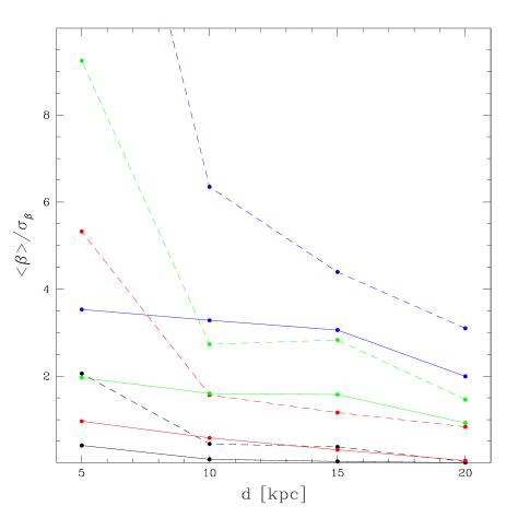
Figure 8: Significance ($\langle\beta\rangle/\sigma_{\beta}$) of the anisotropy detection as a function of the cluster distance. Black, red, green and blue lines indicate simulations of GCs with masses $log(M/M_{\odot})$=4.5, 5, 5.5 and 6, respectively. Solid lines indicate estimates done using only stars with all the three velocity components, dashed lines indicate estimates done using all stars with available proper motions.

In the above test we used only stars brighter than $g<17$ with both proper motions and LOS velocities. These two observables are however derived from completely different techniques and are subject to different sources of uncertainties. For instance, proper motions are measured in terms of angular motions and require an estimate of the cluster distance to be converted into physical units, at odds with radial velocities coming from the observed Doppler-shift of spectroscopic lines. Moreover, because of the different techniques, the estimated velocity errors (essential to properly calculate intrinsic velocity dispersions) can present different systematic biases. So, we considered also the case where only proper motions are available. In this case we considered the quantity

$$\beta^{\prime\prime}=1-\frac{\sigma_{t^{\prime}}^{2}}{\sigma_{r^{\prime}}^{2}}$$

Although the part of the information coming from radial velocities is lost in the above parameter ($\beta^{\prime\prime}$ is a worse estimator of $\beta$ than $\beta^{\prime}$), its corresponding uncertainty is smaller since i) it is given by the propagation of a smaller number of uncertainties, and ii) many more stars can be used to compute $\beta^{\prime\prime}$ (down to $g<20$). The significance level of this approach for the different adopted masses and distances is overplotted in Fig. 8. It is apparent that this last approach provides a larger significance level: although at large heliocentric distances significant detections remain restricted to the most massive GCs, at distances $<$6 kpc it seems possible to detect signatures of anisotropy also in less massive clusters ($log(M/M_{\odot})>5$).

It has been shown (see Sect. 4) that the level of anisotropy changes with radius both in models and in N-body simulations. So, the values of $\beta^{\prime}$ and $\beta^{\prime\prime}$, which are averages over stars sampled at different distance from the cluster center, cannot provide a fair indication of the characteristics (strength, radial profile, etc.) of the cluster anisotropy. A lager number of proper motions covering the entire cluster extent are needed for this purpose.

6 Summary

The comparisons presented in Sect. 4 show that multi-mass models can qualitatively reproduce the radial distribution and velocity dispersion of stars with different masses in GCs subject to frequent collisions during a wide range of their dynamical evolution. In particular, the formulation by Gunn & Griffin (1979; $\alpha$=1) is able to provide a fair representation of N-body simulations after a timescale comparable to the half-mass relaxation time. By looking at Milky Way GCs this condition is satisfied by all but three GCs (namely $\omega$ Cen, Pal 14 and NGC2419; see McLaughlin & van der Marel 2005; Marin-Franch et al. 2009). During the initial half-mass relaxation time multi-mass models overestimate the status of relaxation predicting an unrealistic level of mass segregation. In this case, a simple generalization of the Gunn & Griffin (1979) formalism (adopting $A_{i}\propto m_{i}^{\alpha}$) provides models accounting for intermediate levels of relaxation which better reproduce the simulation properties. As a note of caution, consider that the N-body simulations used here start without any degree of primordial mass segregation which appears to be present in many young massive clusters (de Grijs et al. 2002; Frank, Grebel & Küpper 2014). After many relaxation times the analysed simulations undergo strong mass segregation which is not reached by multi-mass models which slightly underpredict the mass segregation present in the cluster. Both the considered simulations quickly develop two opposite velocity anisotropy trends which cannot be reproduced by analytic models. In the Gunn & Griffin (1979) formalism only radially anisotropic velocity distributions can be simulated in King-Michie models, but alternative formulations exist to account for tangentially anisotropic ones (see e.g. Weinberg 1991; An & Evans 2006). However, the simple dependence of the King-Michie distribution function from angular momentum per unit mass cannot reproduce the wide range of trends of the anisotropy parameter $\beta$ with stellar masses observed in N-body simulations. New models need to be developed to model this quantity in real GCs.

Besides the above considerations, we tested the accuracy of simple fits of the generally available observables (projected number density profiles from RGB+bright MS stars, LOS velocities of RGB stars, MF estimated in a spatially restriced region) with analytic models in the estimate of mass and MF. It appears that the adoption of single-mass models to model GCs after many half-mass relaxation times (as widely done in many past studies because of the lack of information on the cluster MF) can lead to underestimates of their masses up to $\sim$50%. This is likely the reason why dynamical masses estimated in early studies resulted smaller than luminous ones (Mieske et al. 2008). The same conclusion has been reached by SG15 who quantified the bias in the mass estimated from integrated properties of a set of multi-mass GCs models if mass segregation is neglected and found that this effect can lead to a mass underestimate ranging from $0.25<M_{obs}/M_{true}<1$ depending on the metallicity, the MF and the retention fraction of dark remnants (see their Fig. 3). In the same way, the use of multi-mass King-Michie models (with $\alpha=1$) in dynamically young GCs produces the opposite bias leading to a significant overestimate of the cluster mass. In this case, the adoption of models accounting for an intermediate level of relaxation ($0<\alpha<1$) provides better results, although it requires the measure of the MF in two different radial ranges. Both the central cluster region and the outskirts are regions sensitive to the uncertain distribution of heavy objects (like neutron stars, black holes and binaries) and tidal heating. In this respect, tidal heating can be effective in increasing the velocity dispersion even close to the half-mass radius and therefore the estimated mass (as already found by Küpper et al. 2010). An analysis devoted to the derivation of GCs masses should therefore be restricted to a relatively narrow portion of the cluster ($r_{h}/2<r<r_{h}$) to minimize the impact of the above mentioned effects. In the simulations considered here, the adoption of different samples of stars and the location of the deep field used to measure the MF do not significantly affect the mass estimation if multi-mass models are considered. This is due to the relatively good representation of the mass segregation process provided by multi-mass models.

The estimate of the MF is instead less affected by the uncertainties in the density profile and the level of relaxation. However, in strongly mass segregated clusters the MF slope can be underestimated by $\Delta\alpha_{MF}\sim 0.4$ if the local MF is measured at the cluster center. This is due to the inadequacy of multi-mass King-Michie models in reproducing the relative distribution of low/high mass stars in the central region of such relaxed GCs. Note that both the most extensive works on the estimation of the MF slopes (Paust et al. 2010; Sollima et al. 2012) are based on MF estimated from the same dataset of HST observations in the central region of GCs being potentially affected by this bias. This effect is however negligible in those dynamically young clusters where multi-mass King-Michie models do a good job in reproducing the radial distribution of different masses. It is not clear how many GCs of the above mentioned studies can suffer from this bias. On the other hand, the MF measured at the projected half-mass radius (without the application of any correction) is already a fairly good representation of the cluster global MF (see also Pryor et al. 1986, Vesperini & Heggie 1997; Baumgardt & Makino 2003). So, studies based on MF estimated at the half-mass radius (like those by Piotto et al. 1997 and Piotto & Zoccali 1999) can provide good estimates of the global MF, provided that a good estimate of the half-mass radius is available.

A limitation of the approach adopted here is that the clusters simulated in our N-body simulations are a factor of 5-10 smaller than real GCs. Since the effects of stellar evolution, relaxation and tidal effects on the dynamical evolution of the cluster act on different timescales and their efficiencies depend on the cluster mass in different ways, it is not possible to adopt some sort of scaling to GC-size objects (see Baumgardt 2001). We recall that the simulations analysed here consider two extreme situations: while simulation W5rh1R8.5 is a system undergoing quick core-collapse, simulation W5rh11.5R8.5 is dynamically young and subject to a relatively strong tidal field during all its evolution. Thus, we expect that these simulations bracket the whole sample of possible evolutions occurring in GCs. Anyway, any comparison with N-body simulations cannot be used to draw general conclusions on the dynamical properties of real GCs. Further studies on real GCs stars are needed to assess the validity of the results presented here.

We explored the possibility to detect the presence and the characteristics of anisotropy in GCs using the proper motions provided by Gaia. We find that moderate levels of anisotropy (like those naturally developed by N-body simulations) can be detected in massive ($log(M/M_{\odot})\sim 6$) GCs at distances $<$20 kpc and in intermediate-mass GCs ($log(M/M_{\odot})>5$) GCs at $d<6$ kpc. By looking at the Harris catalog (Harris 1996; 2010 edition) there are 25 GCs in this radial/mass range. Unfortunately, with the information provided by Gaia only, it will not be possible to sample the number of objects needed to construct anisotropy profiles even for the nearest GCs. Indeed, the limiting magnitude and the spatial resolution of Gaia will allow to obtain proper motions with errors better than $\sigma_{v}<2~{}km/s$ only for RGB stars in the outskirts of GCs. Nevertheless, Gaia data will be complemented by HST proper motions of stars in the central regions of GCs thus providing the needed coverage for these kind of studies.

References

- Aarseth (1999) Aarseth S. J., 1999, PASP, 111, 1333
- An & Evans (2006) An J. H., Evans N. W., 2006, AJ, 131, 782
- An, Evans, & Deason (2012) An J., Evans N. W., Deason A. J., 2012, MNRAS, 420, 2562
- Anderson & van der Marel (2010) Anderson J., van der Marel R. P., 2010, ApJ, 710, 1032
- Baumgardt (2001) Baumgardt H., 2001, MNRAS, 325, 1323
- Baumgardt & Makino (2003) Baumgardt H., Makino J., 2003, MNRAS, 340, 227
- Bellini et al. (2014) Bellini A., et al., 2014, ApJ, 797, 115
- Bellini, van der Marel, & Anderson (2013) Bellini A., van der Marel R. P., Anderson J., 2013, MmSAI, 84, 140
- Carballo-Bello et al. (2012) Carballo-Bello J. A., Gieles M., Sollima A., Koposov S., Martínez-Delgado D., Peñarrubia J., 2012, MNRAS, 419, 14
- Chen et al. (2014) Chen Y., Girardi L., Bressan A., Marigo P., Barbieri M., Kong X., 2014, MNRAS, 444, 2525
- Da Costa & Freeman (1976) Da Costa G. S., Freeman K. C., 1976, ApJ, 206, 128
- de Grijs et al. (2002) de Grijs R., Gilmore G. F., Johnson R. A., Mackey A. D., 2002, MNRAS, 331, 245
- Djorgovski (1993) Djorgovski S., 1993, ASPC, 50, 373
- Frank, Grebel, Küpper (2014) Frank M. J., Grebel E. K., Küpper A. H. W., 2014, MNRAS, 443, 815
- Fukushige & Heggie (2000) Fukushige T., Heggie D. C., 2000, MNRAS, 318, 753
- Giersz & Heggie (2009) Giersz M., Heggie D. C., 2009, MNRAS, 395, 1173
- Giersz & Heggie (2011) Giersz M., Heggie D. C., 2011, MNRAS, 410, 2698
- Giersz, Heggie, & Hurley (2008) Giersz M., Heggie D. C., Hurley J. R., 2008, MNRAS, 388, 429
- Gunn & Griffin (1979) Gunn J. E., Griffin R. F., 1979, AJ, 84, 752
- Harris (1986) Harris W. E., 1996, AJ, 112, 1487
- Heggie (2014) Heggie D. C., 2014, MNRAS, 445, 3435
- Hurley, Pols, & Tout (2000) Hurley J. R., Pols O. R., Tout C. A., 2000, MNRAS, 315, 543
- Kimmig et al. (2014) Kimmig B., Seth A., Ivans I. I., Strader J., Caldwell N., Anderton T., Gregersen D., 2014, AJ, in press, arXiv:1411.1763
- King (1966) King I. R., 1966, AJ, 71, 64
- King & Anderson (2001) King I. R., Anderson J., 2001, ASPC, 228, 19
- Kroupa (2001) Kroupa P., 2001, MNRAS, 322, 231
- Kruijssen & Mieske (2009) Kruijssen J. M. D., Mieske S., 2009, A&A, 500, 785
- Küpper et al. (2010) Küpper A. H. W., Kroupa P., Baumgardt H., Heggie D. C., 2010, MNRAS, 407, 2241
- Lamers, Baumgardt, & Gieles (2013) Lamers H. J. G. L. M., Baumgardt H., Gieles M., 2013, MNRAS, 433, 1378
- Lane et al. (2010) Lane R. R., et al., 2010, MNRAS, 406, 2732
- Lynden-Bell (1967) Lynden-Bell D., 1967, MNRAS, 136, 101
- Lynden-Bell & Wood (1968) Lynden-Bell D., Wood R., 1968, MNRAS, 138, 495
- Mamon & Boué (2010) Mamon G. A., Boué G., 2010, MNRAS, 401, 2433
- Mandushev, Staneva, & Spasova (1991) Mandushev G., Staneva A., Spasova N., 1991, A&A, 252, 94
- Marigo et al. (2008) Marigo P., Girardi L., Bressan A., Groenewegen M. A. T., Silva L., Granato G. L., 2008, A&A, 482, 883
- Marín-Franch et al. (2009) Marín-Franch A., et al., 2009, ApJ, 694, 1498
- McLaughlin et al. (2006) McLaughlin D. E., Anderson J., Meylan G., Gebhardt K., Pryor C., Minniti D., Phinney S., 2006, ApJS, 166, 249
- McLaughlin & van der Marel (2005) McLaughlin D. E., van der Marel R. P., 2005, ApJS, 161, 304
- Merritt (1981) Merritt D., 1981, AJ, 86, 318
- Mieske et al. (2008) Mieske S., et al., 2008, A&A, 487, 921
- Miocchi et al. (2013) Miocchi P., et al., 2013, ApJ, 774, 151
- Ogorodnikov, Nezhinskii, & Osipkov (1978) Ogorodnikov K. F., Nezhinskii E. M., Osipkov L. P., 1978, BITA, 14, 284
- Oh & Lin (1992) Oh K. S., Lin D. N. C., 1992, ApJ, 386, 519
- Pancino, Bellazzini, & Marinoni (2013) Pancino E., Bellazzini M., Marinoni S., 2013, MmSAI, 84, 83
- Paust et al. (2010) Paust N. E. Q., et al., 2010, AJ, 139, 476
- Piotto, Cool, & King (1997) Piotto G., Cool A. M., King I. R., 1997, AJ, 113, 1345
- Piotto & Zoccali (1999) Piotto G., Zoccali M., 1999, A&A, 345, 485
- Pryor & Meylan (1993) Pryor C., Meylan G., 1993, ASPC, 50, 357
- Pryor, Smith, & McClure (1986) Pryor C., Smith G. H., McClure R. D., 1986, AJ, 92, 1358
- Sarajedini et al. (2007) Sarajedini A., et al., 2007, AJ, 133, 1658
- Schwarzschild (1979) Schwarzschild M., 1979, ApJ, 232, 236
- Shanahan & Gieles (2015) Shanahan R. L., Gieles M., 2015, MNRAS, 448, L94
- Sollima, Bellazzini, & Lee (2012) Sollima A., Bellazzini M., Lee J.-W., 2012, ApJ, 755, 156
- Spitzer & Shull (1975) Spitzer L., Jr., Shull J. M., 1975, ApJ, 201, 773
- Strader, Caldwell, & Seth (2011) Strader J., Caldwell N., Seth A. C., 2011, AJ, 142, 8
- Strader et al. (2009) Strader J., Smith G. H., Larsen S., Brodie J. P., Huchra J. P., 2009, AJ, 138, 547
- Trenti & van der Marel (2013) Trenti M., van der Marel R., 2013, MNRAS, 435, 3272
- van de Ven et al. (2006) van de Ven G., van den Bosch R. C. E., Verolme E. K., de Zeeuw P. T., 2006, A&A, 445, 513
- Vasiliev (2013) Vasiliev E., 2013, MNRAS, 434, 3174
- Vesperini & Heggie (1997) Vesperini E., Heggie D. C., 1997, MNRAS, 289, 898
- Watkins (2015) Watkins. L. L., van der Marel R. P., Bellini A., Anderson J., 2015, ApJ, in press, arXiv:1502.00005
- Weinberg (1991) Weinberg M. D., 1991, ApJ, 368, 66
- Zocchi, Bertin, & Varri (2012) Zocchi A., Bertin G., Varri A. L., 2012, A&A, 539, AA65