Equilibration and GGE for hard wall boundary conditions

Abstract

In this work we present an analysis of a quench for the repulsive Lieb-Liniger gas confined to a large box with hard wall boundary conditions. We study the time average of local correlation functions and show that both the quench action approach and the GGE formalism are applicable for the long time average of local correlation functions. We find that the time average of the system corresponds to an eigenstate of the Lieb-Liniger Hamiltonian and that this eigenstate is related to an eigenstate of a Lieb-Liniger Hamiltonian with periodic boundary conditions on an interval of twice the length and with twice as many particles (a doubled system). We further show that local operators with support far away from the boundaries of the hard wall have the same expectation values with respect to this eigenstate as corresponding operators for the doubled system. We present an example of a quench where the gas is initially confined in several moving traps and then released into a bigger container, an approximate description of the Newton cradle experiment. We calculate the time average of various correlation functions for long times after the quench.

Introduction. Nonequilibrium many body physics is one of the most challenging areas of research of modern condensed matter physics. There have been spectacular advances in the field, driven by experimental studies of dynamics in optically trapped atomic gas systems, systems with extremely weak coupling to the environment allowing a study of essentially Hamiltonian dynamics of time evolution key-5-1 (1, 3, 2, 4, 6, 7, 8, 9, 5). Encouraged by these experimental advances there has been great theoretical activity in the area key-12 (10, 11, 12, 13, 14, 15, 16, 17, 18, 19, 20), focused on questions like does a steady state emerge, how do local observables equilibrate, is there any principle which allows us to relate the steady state to the initial conditions?

One of the most important recent experimental key-5-1 (1, 21) and theoretical key-10 (22, 24, 26, 33, 34, 27, 28, 29, 30, 31, 32, 23, 25) results is that there is a relation between the initial state and the long time steady state for time evolution of integrable models. This was ascribed to the fact that integrable models possess an infinite family of local conserved charges $\left\{I_{i}\right\}$, in involution, which include the Hamiltonian $H$, typically identified with $I_{2}$:

$$\left[H,I_{i}\right]=\left[I_{i},I_{i^{\prime}}\right]=0,\,H=I_{2},$$ (1)

These conserved quantities imply that there is a complete set of eigenstates for an integrable model which may be parametrized by sets of rapidities $\left\{k_{i}\right\}$ which are simultaneous eigenstates of all $I_{i}$. For the Lieb-Liniger Hamiltonian, the model which describes the Newton Cradle experiment key-5-1 (1), the the action of the charges on these eigenstates given by: $I_{i}\left|\left\{k\right\}\right\rangle=\sum k^{i}\left|\left\{k\right\}\right\rangle$. It was shown for the Lieb-Liniger gas, by following its actual time evolution numerically and analytically, key-10 (22), that at long times the gas reaches equilibration with the density matrix having no time dependence and becoming diagonal in the basis $\left\{k_{i}\right\}$.

How to describe this diagonal, time independent, density matrix in general is an open question. It was proposed that the diagonal ensemble in turn key-10 (22, 24) takes the form of a generalized Gibbs ensemble (GGE) key-31 (35, 25, 26, 24, 33, 34, 27, 28, 29, 30, 31, 32, 36),

$$\rho_{GGE}=\frac{1}{Z}\exp\left(-\sum\alpha_{i}I_{i}\right)$$ (2)

with the $\alpha_{i}$, the generalized inverse temperatures, encoding the initial state $\left|\Phi_{0}\right\rangle$ through the requirement $\langle I_{i}\rangle_{final}\equiv Tr\left\{\rho_{GGE}I_{i}\right\}=\left\langle\Phi_{0}\left|I_{i}\right|\Phi_{0}\right\rangle\equiv\langle I_{i}\rangle_{initial}$. $Z$ is a normalization constant insuring $Tr\left[\rho_{GGE}\right]=1$. This interesting proposal, while valid for the case at hand, the repulsive Lieb-Liniger model, fails for models with bound states (string solutions) key-46 (37), a large class of models which encompasses, among others, the attractive Lieb-Liniger, the XXZ Heisenberg chain and the Hubbard model.

When a GGE description is valid it provides an elegant shortcut to the computation of correlation functions at long times, without having to explicitly follow the time evolution or to compute overlaps. Instead, having reached equilibration the correlation functions (of the Lieb-Liniger gas) at long times, or in this case the time average of the correlation functions, may be computed by taking their expectation value with respect to the GGE density matrix, e.g. $\left\langle\Theta\left(t\rightarrow\infty\right)\right\rangle=Tr\left[\rho_{GGE}\Theta\right]$. It was further shown key-1 (38) that the GGE ensemble is equivalent to an eigenstate, $\rho_{GGE}\cong\left|\left\{k_{0}\right\}\right\rangle\left\langle\left\{k_{0}\right\}\right|$, for an appropriately chosen $\left|\left\{k_{0}\right\}\right\rangle$ so that $\left\langle\Theta\left(t\rightarrow\infty\right)\right\rangle=\left\langle\left\{k_{0}\right\}\right|\Theta\left|\left\{k_{0}\right\}\right\rangle$. Another approach, the quench action approach key-52 (39), is of more general validity but is more difficult to implement. It allows the computation of the diagonal density matrix in terms of the overlaps of eigenstates with the initial state, but such overlaps are hard to determine and are known only for few initial states. Again, it was shown that the resulting diagonal ensemble is equivalent to an eigenstate.

Most of the work done on the Lieb-Liniger model was concerned with periodic boundary conditions, exceptions are key-50 (40). Real systems key-5-1 (1, 3, 2, 4, 6, 7, 8, 9, 5) have finite extent with typically a parabolic potential confining the particles. We will approximate this parabolic confining potential as a hard wall boundary. We will study the system in the limit where the system size $L\rightarrow\infty$, the number of particles $N$ scales with the system size, $N/L=const$, and for times much greater then the system size, $t>L/v_{typ}$ ($v_{typ}$ is a typical velocity). This regime is relevant for many experiments. We note that this time scale has been theoretically considered for the Tonks gas before key-49 (41, 40).

Time average. We shall consider circumstances where the system does not necessarily equilibrate in the long time limit and focus instead on the long time average of a local operator (observable) $\Theta$ evolving from the initial state $\left|\Psi\right\rangle$,

$$\begin{array}[t]{l}\left\langle\Theta\right\rangle_{T}\equiv\frac{1}{T}\int_{0}^{T}dt\left\langle\Psi\right|e^{iH_{LL}t}\Theta e^{-iH_{LL}t}\left|\Psi\right\rangle=\\ =\frac{1}{T}\sum_{\lambda}\sum_{\kappa}\frac{e^{i\left(E_{\lambda}-E_{\kappa}\right)T}-1}{i\left(E_{\lambda}-E_{\kappa}\right)}\left\langle\Psi\mid\lambda\right\rangle\left\langle\lambda\right|\Theta\left|\kappa\right\rangle\left\langle\kappa\mid\Psi\right\rangle\\ \cong\sum_{\lambda}\left\langle\Psi\mid\lambda\right\rangle\left\langle\lambda\right|\Theta\left|\lambda\right\rangle\left\langle\lambda\mid\Psi\right\rangle,\end{array}$$ (3)

we find it is given by a diagonal ensemble in the limit $T\rightarrow\infty$. Therefore the time averaged expectation values of local observables is given by the diagonal ensemble. Here $\left|\lambda\right\rangle$ and $\left|\kappa\right\rangle$ are exact eigenstates of the system in the box.

The system we shall study is the Lieb-Liniger Hamiltonian describing the 1-D system of bosons with short range interactions key-31 (35, 42, 43):

$$H_{LL}=\intop_{0}^{L}dx\left\{\partial_{x}b^{\dagger}\left(x\right)\partial_{x}b\left(x\right)+c\left(b^{\dagger}\left(x\right)b\left(x\right)\right)^{2}\right\}.$$ (4)

Here $b^{\dagger}\left(x\right)$ is the bosonic creation operator at the point $x$ and $c$ is the coupling constant. Hard wall boundary conditions are imposed:

$$\psi\left(x_{1}=0,x_{2},...x_{N}\right) =0$$

$$\psi\left(x_{1},x_{2},..x_{N}=L\right) =0$$ (5)

with $\psi\left(x_{1},...x_{N}\right)$ the wave function of the bosons in the region $x_{1}<x_{2}<...<x_{N}$.

The exact eigenstates of the Hamiltonian with the boundary conditions given in Eq. (5) are given by key-43 (42):

$$\psi\left(\left|k_{1}\right|,..\left|k_{N}\right|\right)=\sum_{\left\{\varepsilon\right\}}C\left\{\varepsilon\right\}\bar{\psi}\left(\varepsilon_{1}\left|k_{1}\right|,..\varepsilon_{N}\left|k_{N}\right|\right),$$ (6)

where $\left\{\varepsilon\right\}$ corresponds to the $2^{N}$ sequences $\varepsilon_{j}=\pm 1$ and $C\left(\varepsilon_{1},...\varepsilon_{N}\right)=\prod\varepsilon_{j}\prod_{i<j}\left(1-\frac{ic}{\varepsilon_{i}\left|k_{i}\right|+\varepsilon_{j}\left|k_{j}\right|}\right)$, and

$$\bar{\psi}\left(k_{1},...k_{N}\right)=\sum_{P}A\left(P\right)e^{i\sum k_{P_{i}}x_{i}},\quad x_{1}<x_{2}<...<x_{N}$$

with $A\left(P\right)=\prod_{i<j}\left(1+\frac{ic}{k_{P_{i}}-k_{P_{j}}}\right)$ and the sum $\sum_{P}$ extending over $N!$ permutations. These are the eigenstates with periodic boundary conditions. Furthermore the rapidities $k_{i}=\varepsilon_{i}\left|k_{i}\right|$ satisfy the Bethe ansatz equations key-43 (42):

$$k_{i}L=\pi n_{i}+\sum_{j\neq i}\left(\arctan\left(\frac{c}{k_{i}-k_{j}}\right)+\arctan\left(\frac{c}{k_{i}+k_{j}}\right)\right)$$

These are exactly the same equations as for a doubled system of length $2L$ with twice as many particles having $2N$ with rapidities $\left\{\varepsilon_{i}\left|k_{i}\right|\right\}$. There is a one to one correspondence between states of a system with hard wall boundary conditions and states of a doubled system with periodic boundary conditions where all the rapidities come in pairs $\left\{k,-k\right\}$ key-43 (42). The Bethe Ansatz equations which determine the allowed rapidities $\{k\}$ for the doubled system can be translated in a standard fashion key-31 (35) into a set of integral equations for the rapidities’ densities. We denote, for a given eigenstate $\left|\left\{k\right\}\right\rangle$ of the doubled system, by $\rho_{p}\left(k\right)$ the Bethe density of particles so that $2L\rho_{p}\left(k\right)dk$ is the number of particles in the interval $\left[k,k+dk\right]$ of the doubled system. Similarly $\rho_{h}\left(k\right)$ denotes the hole density and $\rho_{t}\left(k\right)=\rho_{p}\left(k\right)+\rho_{h}\left(k\right)$ the total density. The number of states $\left|\left\{k\right\}\right\rangle$, consistent with a given set of densities, $\{\rho_{p}\left(k\right),\rho_{h}\left(k\right)\}$, is measured by the Yang-Yang entropy key-31 (35), $S_{YY}\left(\left\{\rho\right\}\right)=\int_{-\infty}^{\infty}dk\left(\rho_{h}\left(k\right)\ln\left(\frac{\rho_{t}\left(k\right)}{\rho_{h}\left(k\right)}\right)+\rho_{p}\left(k\right)\ln\left(\frac{\rho_{t}\left(k\right)}{\rho_{p}\left(k\right)}\right)\right)$. The densities $\{\rho_{p}\left(k\right),\rho_{h}\left(k\right)\}$ for the doubled system are determined by the thermodynamic Bethe Ansatz equations which enforce the periodic boundary conditions: $\rho_{t}\left(k\right)=\frac{1}{2\pi}+\frac{1}{2\pi}\int K\left(k,q\right)\rho_{p}\left(q\right)$, with $K\left(k,q\right)=\frac{2c}{c^{2}+\left(k-q\right)^{2}}$.

Time average, quench action and GGE action. The time average of a local observable, Eq.(3), can be rewritten as key-44 (44, 39):

$$\left\langle\Theta\right\rangle_{T\rightarrow\infty}=\int D\left(\frac{\rho_{t}}{\rho_{p}}\right)e^{2LS_{Quench}\left(\left\{\rho\left(k\right)\right\}\right)}\left\langle\left\{k\right\}\right|\Theta\left|\left\{k\right\}\right\rangle$$ (7)

Here $\left\langle\left\{k\right\}\right|\Theta\left|\left\{k\right\}\right\rangle$ is computed in the hard wall (non-doubled) system, and the quench action is given by:

$$S_{Quench}\left(\left\{\rho\left(k\right)\right\}\right)=\int g^{\Phi}\left(k\right)\rho\left(k\right)+\frac{1}{2}S_{YY}\left(\left\{\rho\left(k\right)\right\}\right)$$

with $\int g^{\Phi}\left(k\right)\rho\left(k\right)=\frac{2}{2L}\log\left(\left|\left\langle\Phi\mid\left\{k\right\}\right\rangle\right|\right)$, where $g\left(k\right)=g\left(-k\right)$. The extra factor of $\frac{1}{2}$ in front of $S_{YY}\left(\left\{\rho\left(k\right)\right\}\right)$ comes from the fact that we are only considering states where the rapidities come in pairs $\left\{k,-k\right\}$.

The time average of the Lieb-Liniger gas with hard wall boundary conditions corresponds therefore to a single eigenstate the one that maximizes the quench action key-44 (44). Let us denote solution quasiparticle density for the doubled system as $\rho_{p}^{\Phi}\left(k\right)$ and the quasiparticle density for the original system as $\tilde{\rho}_{p}^{\Phi}\left(k\right)$ with $\tilde{\rho}_{p}^{\Phi}\left(k\right)=2\theta\left(k\right)\rho_{p}^{\Phi}\left(k\right)$ and $\rho_{p}^{\Phi}\left(k\right)=\rho_{p}^{\Phi}\left(-k\right)$.

We proceed to convert the quench action into a GGE description of the system with hard wall boundary conditions and use it to compute time average of local observables. We begin by determining its conserved charges. Since an eigenstate, see Eq. (6) is given by a superposition of rapidities of the form $\left\{\varepsilon_{i}\left|k_{i}\right|\right\}$ all the even conserved quantities satisfy the relation:

$$I_{2n}\psi\left(\left|k_{1}\right|,..\left|k_{N}\right|\right)=\sum k_{i}^{2n}\psi\left(\left|k_{1}\right|,..\left|k_{N}\right|\right)$$ (8)

Therefore $\left\{I_{2n}\right\}$ form a set of local integrals of motion and the quasiparticle density $\rho_{p}^{\Phi}\left(k\right)$ being symmetric in $k$ is, in turn, uniquely determined by its even moments which correspond to its conserved quantities key-54 (45) in particular $\left\{I_{2n}\right\}$ are complete. Hence the even local integrals of motion, $\left\{I_{2n}\right\}$, determine final state in terms of the GGE density operator, $\tilde{\rho}_{GGE}=\frac{1}{Z}\exp\left(-\sum\alpha_{2n}I_{2n}\right)$. The inverse temperatures, $\alpha_{2n}$, found from the initial state $|\Phi\rangle$ setting $\left\langle I_{2n}\right\rangle=\left\langle I_{2n}\right\rangle_{GGE}$. Any local observable can be written in the form:

$$\left\langle\Theta\right\rangle_{GGE}=\int D\left(\frac{\rho_{t}}{\rho_{p}}\right)e^{2LS_{GGE}\left(\left\{\rho\left(k\right)\right\}\right)}\left\langle\left\{k\right\}\right|\Theta\left|\left\{k\right\}\right\rangle$$ (9)

with $S_{GGE}=\int\rho\left(k\right)\left(\frac{1}{2}\sum\alpha_{2n}k^{2n}+\frac{1}{2L}\ln Z\right)+\frac{1}{2}S_{YY}$. We can identify $g\left(k\right)=\frac{1}{2}\sum\alpha_{2n}k^{2n}+\frac{1}{2L}\ln Z$ (since both the quench action and the GGE are equivalent to a single eigenstate of the Lieb Liniger Hamiltonian (which corresponds to the extremum of the path integral in Eq. (9)), we establish that $\left\langle\Theta\right\rangle_{T\rightarrow\infty}=\left\langle\Theta\right\rangle_{GGE}$. We conclude that the time average of Lieb-Liniger gas corresponds to a GGE density matrix where the conserved operators are the even local conserved densities. We further note that when considering an operator $\Theta$ with support far away from from the hard wall boundaries we may as well calculate $\left\langle\Theta\right\rangle_{GGE}$ with respect to the doubled system. Indeed $\left\langle\Theta\right\rangle_{GGE}=Tr\left\{\Theta\exp\left(-\sum\alpha_{2n}I_{2n}\right)\right\}$ for both systems. Since operators $I_{2n}$ are local, all correlation functions $\Theta$ may be calculated by considering paths where the propagator is the quadratic piece of $\sum\alpha_{2n}I_{2n}$ while the interactions are given by the quartic and higher order pieces. We note that paths that cross the boundary of the system are exponentially suppressed when $\Theta$ is far from the boundary.

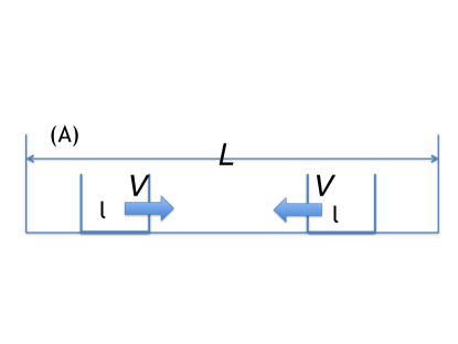
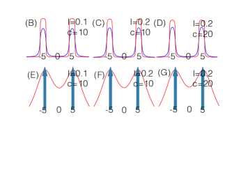
Figure 1: (A) The system is initialized in a state where two hard wall Lieb Liniger droplets of length $L_{i}$ moving with velocity $\pm V$ inside a large hard wall trap of length $L$. (B-G) The velocity distribution for the BEC bottom and the ground state quench top for a variety of quasiparticle densities and interaction strengths. The time average velocity distribution in red the initial velocity distribution before the quench is shown in blue. (B-D) $V=5$, $L=1$, $k_{F}=1$. (E-G) $V=5$, $L=1$ $n=1$. The initial velocity distribution is computed in the supplementary online information and is shown in blue while the final velocity distribution is shown in red. the initial velocity distribution of the BEC is shown in the form of delta functions. Note collision narrowing in (B-D) and broadening in (E-G).

Examples: 1. Newton’s cradle type - eigenstate initial conditions. We will consider the following setup: there is a large trap of length $L$ with hard wall boundary conditions in which there are multiple smaller traps of lengths $L_{i}$ moving with velocities $V_{i}$. Each of the smaller traps contains a Lieb-Liniger gas initialized in an eigenstate described by quasiparticle density $\rho_{p}^{i}\left(k\right)$ with $\rho_{p}^{i}\left(k\right)=\rho_{p}^{i}\left(-k\right)$ (we note that thermal states also correspond to specific eigenstates key-31 (35)). At time $t=0$ the smaller traps are turned off and the whole of the gas expands into the larger trap. We would like to find the quasiparticle density of the long time averaged final state. To do so we use the fact that all the even local conserved quantities are conserved during the quench, so we need to equate their values before and after the quench. We will show in the supplementary online information that in the thermodynamic limit we do not need to consider the edge effects for computing the local conserved quantities. Therefore we need to find a symmetric quasiparticle density that satisfies the following set of equations:

$$L\int dk\rho_{p}^{f}\left(k\right)k^{2n}=\sum L_{i}\int\rho_{p}^{i}\left(k\right)\left(k+\frac{1}{2}V_{i}\right)^{2n}$$

The extra terms $k+\frac{1}{2}V_{i}$ stem from the fact that under a boost to velocity $V_{i}$ the wave function is multiplied by $\exp\left(i\sum m_{i}V_{i}x_{i}\right)$ with $m_{i}=\frac{1}{2}$. We note that here $\rho_{p}^{i}\left(k\right)=\rho_{p}^{i}\left(-k\right)$ is the quasiparticle density of the doubled system. A solution to this equation is given by:

$$\rho_{p}^{f}\left(k\right)=\sum\frac{L_{i}}{2L}\left(\rho_{p}^{i}\left(k+\frac{1}{2}V_{i}\right)+\rho_{p}^{i}\left(k-\frac{1}{2}V_{i}\right)\right),$$

This solution allows for the calculation of various correlation functions for the system. Note that in the case of a periodic boundary condition we would have received the answer $\rho_{p}^{f}\left(k\right)=\sum\frac{L_{i}}{L}\rho_{p}^{i}\left(k-\frac{1}{2}V_{i}\right)$.

Consider now the quench dynamics of a system consisting initially of two boxes of length $l$ with $N$ particles each in the ground state moving with of opposite velocities $V$ and $-V$ see Fig. 1(A). In experiment one typically measures the probability distribution for the particle velocity. It is given by the Fourier transform of the field-field correlation function

$$P\left(v,t\right)=\int dxe^{-i\frac{v}{2}x}\left\langle b^{\dagger}\left(x\right)b\left(0\right)\right\rangle_{t}$$

We will be interested in its time average. This example has many similarities to the experiment done by Kinoshita et. al key-5-1 (1) where the system is placed in a parabolic confining potential and initialized in a state with some of the particles going left and some of the particles going right. Here we have replaced the parabolic confining potential with a hard wall box and do not therefore expect this probability distribution to match well with the one measured in the experiment. The reason being that when confined by a harmonic potential the bosons move up and down the potential which slows them down and speeds them up periodically. In our setup the particles hit a hard wall and have their velocities reversed after the collision (as such they experience no intermediate velocities). As a result our calculation is expected to underestimate the probability of a particle having low velocity.

We now proceed with the calculation: An important ingredient in calculating correlation functions is the occupation probability of the doubled box $f_{L}\left(k\right)=\frac{\rho_{p}\left(k\right)}{\rho_{t}\left(k\right)}$. To calculate it we first calculate the quasiparticle distributions of the smaller boxes. The ground state total density $\rho_{t}$ of the smaller boxes, in the limit of large $c$ is determined from key-31 (35): $2\pi\rho_{t}\left(k\right)=1+\frac{2}{c}\int_{-k_{F}}^{k_{F}}dq\rho_{t}\left(q\right)$ leading to $\rho_{t}\left(k\right)=\theta\left(-k_{F},k_{F}\right)\frac{1}{2\pi}\left(1+\frac{2k_{F}}{\pi c}\right)+o(\frac{k_{F}}{c})....$. Furthermore it is possible to obtain a relation between $k_{F}$ and $N$ with $k_{F}=\frac{\pi N}{l}-\frac{2}{\pi c}\left(\frac{\pi N}{l}\right)^{2}+.....$ which implies that the total particle density of the doubled box is given by: $\rho_{p}\left(k\right)=\frac{l}{2\pi L}\left(1+\frac{2k_{F}}{\pi c}\right)\sum_{v=\pm\frac{V}{2}}\theta\left(-k_{F}+v,k_{F}+v\right)$, therefore the final total density is: $\rho_{t}\left(k\right)=\frac{1}{2\pi}\left(1+\frac{4k_{F}l}{c\pi L}\right)+....$ and occupation probability:

$$f_{L}\left(k\right)=A_{L}\sum_{v=\pm\frac{V}{2}}\theta\left(-k_{F}+v,k_{F}+v\right)$$ (10)

with $A_{L}=\frac{l}{L}\left(1+\frac{2k_{F}}{\pi c}\left(1-\frac{2l}{L}\right)\right)$. We now proceed to compute the field-field correlation function $\left\langle b^{\dagger}\left(x\right)b\left(0\right)\right\rangle$. We will only consider the case when the points $x$ and $0$ are far away from the boundaries of the box so we may use the doubled system for all calculations. In terms of the occupation distribution, $f_{L}(k)$, the correlation function is given by key-53 (46): $\left\langle b^{\dagger}\left(x\right)b\left(0\right)\right\rangle=\int\frac{dk}{2\pi}f_{L}\left(k\right)e^{-ikx}\omega\left(k\right)\exp\left(-x\int duf_{L}\left(t\right)P_{u}\left(k\right)\right)+h.o.t.$ with $\omega\left(k\right)=\exp\left(-\frac{1}{2\pi}\int dqK\left(k,q\right)f\left(q\right)\right)\cong\exp\left(-\frac{F_{L}}{\pi c}\right)$, and $F_{L}=4k_{F}A_{L}$ and $K\left(k,q\right)=\frac{2c}{\left(k-q\right)^{2}+c^{2}}\cong\frac{2}{c}$. The generating function $P_{u}\left(k\right)$ satisfies the equation: $2\pi P_{u}\left(k\right)=-\frac{k-u+ic}{u-k+ic}\exp\left(-\int f_{L}\left(s\right)K\left(u,s\right)P_{s}\left(k\right)\right)-1$ yielding for large $c$: $P_{u}\left(k\right)\cong-\frac{1}{2\pi}\left(1+\exp\left(-\frac{2F_{L}}{\pi c}\right)\right)+i\frac{\exp\left(-\frac{2F_{L}}{\pi c}\right)}{\pi c}\left(k-u\right)$ and $\int f_{L}\left(u\right)P_{u}\left(k\right)\cong-\frac{F_{L}}{2\pi}\left(1+\exp\left(-\frac{2F_{L}}{\pi c}\right)\right)+iF_{L}\frac{k}{\pi c}\exp\left(-\frac{2F_{L}}{\pi c}\right)$. Combing all we obtain the velocity probably distribution:

$$P\left(v\right)\sim A_{L}\frac{\exp\left(-\frac{F_{L}}{\pi c}\right)}{2\pi}\sum_{i,j=\pm}\left(-1\right)^{j}\arctan A_{i,j}(v)$$ (11)

with $A_{\pm\pm}(v)=C_{L}\left((1-F_{L}\frac{\exp\left(-2F_{L}/\pi c\right)}{\pi c})\left(\pm\frac{V}{2}\pm k_{F}\right)+\frac{v}{2}\right)$ and $C_{L}=\frac{2\pi}{4k_{F}A_{L}\left(1+\exp\left(-\frac{2F_{L}}{\pi c}\right)\right)}$.

Note that the velocity distribution Eq.(11), see Fig. 1(B-D), underwent a collision narrowing. The distribution is the leading order term for the set up of a hard wall trap. In a harmonic trap, as argued before, the probability of a particle having low velocity would be larger due to having to move up and down the harmonic confining potential.

2. Newton’s cradle type, BEC initial conditions. A very similar scenario happens when we initialize the state in a collection of BEC’s each of length $L_{i}$ moving with velocity $V_{i}$ inside a larger trap of length $L$. At $t=0$ the smaller traps are released and interactions are turned on so that the system is described by a Lieb-Liniger Hamiltonian with coupling constant $c$. The initial state is BEC and can be described by a quasiparticle density key-44 (44):

$$\rho_{p}^{BEC_{i}}\left(x\right)=\frac{\tau_{i}\frac{d}{d\tau_{i}}a\left(x,\tau\right)}{1+a\left(x,\tau\right)}.$$ (12)

Here $x=\frac{k}{c}$, $\tau_{i}=\frac{n_{i}}{c}$ (where $n_{i}$ is the particle density) and $a\left(x,\tau\right)=\frac{2\pi\tau}{x\sinh\left(2\pi x\right)}J_{1-2ix}\left(4\sqrt{\tau}\right)J_{1+2ix}\left(4\sqrt{\tau}\right)$. With $J_{n}$ a modified Bessel function of the first kind of order $n$. By an argument similar to the one given above the final quasiparticle density is given by:

$$\rho_{p}^{f}\left(k\right)=\sum\frac{L_{i}}{2L}\left(\rho_{p}^{BEC_{i}}\left(k+\frac{1}{2}V_{i}\right)+\rho_{p}^{BEC_{i}}\left(k-\frac{1}{2}V_{i}\right)\right)$$ (13)

More generally any translationally invariant quench that may be solved using periodic boundary conditions it is possible to define a box quench which may be solved analogously to Eq. (13) above. In the supplementary online information we show that for a quench with two boxes (each of length $l$ with $N$ particles in each box in a BEC state) with velocities $V$ and $-V$ inside of a box of total length $L$ the velocity probably distribution is given by:

$$P\left(v\right) \sim nB_{L}\frac{\exp\left(-\frac{G_{L}}{\pi c}\right)}{\pi}\times$$

$$\times\left(\frac{H_{L}}{H_{L}^{2}+\frac{1}{4}\left(v-VK_{L}\right)}+\frac{H_{L}}{H_{L}^{2}+\frac{1}{4}\left(v+VK_{L}\right)}\right)$$

Here, $K_{L}=\left(1-G_{L}\frac{\exp\left(-2G_{L}/\pi c\right)}{\pi c}\right)$, $G_{L}=2nB_{L}$ $B_{L}=\frac{l}{L}\frac{1}{\frac{1}{2\pi}+\frac{2N}{\pi cL}}$, $H_{L}=\frac{G_{L}}{2\pi}\left(1+\exp\left(-\frac{2G_{L}}{\pi c}\right)\right)+2n\left(1-G_{L}\frac{\exp\left(-2G_{L}/\pi c\right)}{\pi c}\right)$ and $n=\frac{N}{l}$. See Fig. 1(E-G).

We note that the average velocity distribution has broadened as compared to its value at the start of the quench, while in the previous case ground state initial conditions the distribution underwent narrowing due to the collisions.

Conclusions. We have studied a quench of the Lieb-Liniger gas on an interval with hard wall boundary conditions. We introduced a doubled system with periodic boundary conditions that is equivalent to the one on an interval. We have shown that the GGE formalism applies to the computation of time averages of local operators and that the even integrals of motion form a complete set of local conserved quantities. We have used this approach to compute a quench where there are several small traps inside of a larger one and the smaller traps are released. We found that the quasiparticle density is additive. We have also calculated the expectation values of some local operators for this quench and in particular the time averaged velocity distribution. In the future it would be of interest to extend this work to models with bound states.

Acknowledgments: This research was supported by NSF grant DMR 1410583 and Rutgers CMT fellowship.

Supplementary online information

Correlation functions (zero temperature case)

We would like to calculate various correlation functions $\left\langle b^{\dagger}\left(0\right)b^{\dagger}\left(0\right)b\left(0\right)b\left(0\right)\right\rangle$, $\left\langle b^{\dagger}\left(0\right)b^{\dagger}\left(0\right)b^{\dagger}\left(0\right)b\left(0\right)b\left(0\right)b\left(0\right)\right\rangle$, and $\left\langle\rho\left(x\right)\rho\left(0\right)\right\rangle$ ($\left\langle b^{\dagger}\left(x\right)b\left(0\right)\right\rangle$ and the quasiparticle occupation probability $f_{L}\left(k\right)=\frac{\rho_{p}\left(k\right)}{\rho_{t}\left(k\right)}$ has already been partially done in the main text) for quenches discussed in the main text. We will consider the case where both $x$ and $0$ are far away from the boundaries of the box. In this case the problem becomes translationally invariant and all correlations may be calculated using a doubled box with doubled quasiparticle density (see the discussion below Eq. (9) in the main text). As such we may use the results found in key-49-1 (47, 48, 49, 50, 46). We will consider the initial conditions where the system starts with two small boxes of length $l$ with $N$ particles each, with each box cooled to the ground state. We will also assume that the boxes have velocities $V$ and $-V$. To make the computations tractable we will work only in the limit of large $c$ and only to leading order in $\frac{1}{c}$.

We now compute the local correlation functions using this occupation probability. We begin with the correlation function $\left\langle b^{\dagger}\left(0\right)b^{\dagger}\left(0\right)b\left(0\right)b\left(0\right)\right\rangle$. It is given bykey-49-1 (47):

$$\left\langle b^{\dagger}\left(0\right)b^{\dagger}\left(0\right)b\left(0\right)b\left(0\right)\right\rangle =2\int\frac{dk_{1}}{2\pi}f_{L}\left(k_{1}\right)\int\frac{dk_{2}}{2\pi}f_{L}\left(k_{2}\right)\frac{\left(k_{1}-k_{2}\right)^{2}}{\left(k_{1}-k_{2}\right)^{2}+c^{2}}+....$$

$$\cong\frac{4}{\pi^{2}}A_{L}^{2}k_{F}^{2}\left(\frac{V}{c}\right)^{2}+....$$ (14)

For convenience we will denote $A_{L}=\frac{l}{L}\left(1+\frac{2k_{F}}{\pi c}\left(1-\frac{2l}{L}\right)\right)$. Where the last equality is in the limit $k_{F}\ll V\ll c$. Furthermore it is possible to obtain the density density density correlation function in the same limit. It is given by key-49-1 (47):

$$\left\langle b^{\dagger}\left(0\right)b^{\dagger}\left(0\right)b^{\dagger}\left(0\right)b\left(0\right)b\left(0\right)b\left(0\right)\right\rangle\cong 6\int\frac{dk_{1}}{2\pi}\int\frac{dk_{2}}{2\pi}\int\frac{dk_{3}}{2\pi}f_{L}\left(k_{1}\right)f_{L}\left(k_{2}\right)f_{L}\left(k_{3}\right)\frac{\left(k_{1}-k_{2}\right)^{2}}{\left(k_{1}-k_{2}\right)^{2}+c^{2}}\frac{\left(k_{1}-k_{3}\right)^{2}}{\left(k_{1}-k_{3}\right)^{2}+c^{2}}\frac{\left(k_{2}-k_{3}\right)^{2}}{\left(k_{2}-k_{3}\right)^{2}+c^{2}}$$

$$\cong \frac{1}{8\pi^{3}}A_{L}^{3}\left(\frac{2k_{F}}{c}\right)^{4}\left(\frac{V}{c}\right)^{4}$$ (15)

Where again the last equality is true in the limit $k_{F}\ll V\ll c$.

We now repeat the calculation of the field-field correlation function $\left\langle b^{\dagger}\left(x\right)b\left(0\right)\right\rangle$ (already partly given in the main text). It is given by key-53 (46):

$$\left\langle b^{\dagger}\left(x\right)b\left(0\right)\right\rangle \cong\int\frac{dk}{2\pi}f_{L}\left(k\right)e^{-ikx}\omega\left(k\right)\times$$

$$\times\exp\left(-x\int dtf_{L}\left(t\right)P_{t}\left(k\right)\right)$$

Here $\omega\left(k\right)=\exp\left(-\frac{1}{2\pi}\int dqK\left(k,q\right)f\left(q\right)\right)\cong\exp\left(-\frac{F_{L}}{\pi c}\right)$, where $F_{L}=4k_{F}A_{L}$ and $K\left(k,q\right)=\frac{2c}{\left(k-q\right)^{2}+c^{2}}\cong\frac{2}{c}$. Furthermore the function $P_{t}\left(k\right)$ satisfied the equation:

$$2\pi P_{t}\left(k\right)=-\frac{k-t+ic}{t-k+ic}\exp\left(-\int f_{L}\left(s\right)K\left(t,s\right)P_{s}\left(k\right)\right)-1$$ (16)

Using this expression it is possible to obtain that:

$$P_{t}\left(k\right)\cong -\frac{1}{2\pi}\left(1+\exp\left(-\frac{2F_{L}}{\pi c}\right)\right)$$

$$+i\frac{\exp\left(-\frac{2F_{L}}{\pi c}\right)}{\pi c}\left(k-t\right)$$

From this we obtain that $\int f_{L}\left(t\right)P_{t}\left(k\right)\cong-\frac{F_{L}}{2\pi}\left(1+\exp\left(-\frac{2F_{L}}{\pi c}\right)\right)+i\frac{kF_{L}}{\pi c}\exp\left(-\frac{2F_{L}}{\pi c}\right)$. Combing we obtain that :

$$\left\langle b^{\dagger}\left(x\right)b\left(0\right)\right\rangle =\frac{\exp\left(-\frac{F_{L}}{\pi c}\right)}{2\pi}\exp\left(-\frac{F_{L}x}{2\pi}\left(1+\exp\left(-\frac{2F_{L}}{\pi c}\right)\right)\right)\int f_{L}\left(k\right)e^{-ikx\left(1-F_{L}\frac{\exp\left(-2F_{L}/\pi c\right)}{\pi c}\right)}$$

$$=\frac{2\exp\left(-\frac{F_{L}}{\pi c}\right)}{\pi x\left(1-\frac{\exp\left(-2F_{L}/\pi c\right)}{\pi c}\right)}\exp\left(-\frac{F_{L}x}{2\pi}\left(1+\exp\left(-\frac{2F_{L}}{\pi c}\right)\right)\right)A_{L}\times$$

$$\times\sin\left(k_{F}x\left(1-F_{L}\frac{\exp\left(-2F_{L}/\pi c\right)}{\pi c}\right)\right)\cos\left(\frac{V}{2}x\left(1-F_{L}\frac{\exp\left(-2F_{L}/\pi c\right)}{\pi c}\right)\right)$$ (17)

We now proceed to the density density calculation. We know that the density density function is given by key-52-1 (50):

$$\left\langle\rho\left(x\right)\rho\left(0\right)\right\rangle=\rho^{2}-\frac{1}{4\pi^{2}}\int dk_{1}f_{L}\left(k_{1}\right)\omega\left(k_{1}\right)\int dk_{2}f_{L}\left(k_{2}\right)\omega\left(k_{2}\right)\left(\frac{k_{1}-k_{2}+ic}{k_{1}-k_{2}-ic}\right)\left(\frac{p\left(k_{1},k_{2}\right)}{k_{1}-k_{2}}\right)\exp\left(xp\left(k_{1},k_{2}\right)\right)$$

Here $p\left(k_{1},k_{2}\right)=-i\left(k_{1}-k_{2}\right)+\int dtf_{L}\left(t\right)P_{t}\left(k_{1},k_{2}\right)$. Here the function $P_{t}\left(k_{1},k_{2}\right)$ satisfies:

$$2\pi P_{t}\left(k_{1},k_{2}\right)=\frac{k_{1}-t+ic}{k_{1}-t-ic}\cdot\frac{k_{2}-t-ic}{k_{2}-t+ic}\exp\left(-\int f_{L}\left(s\right)K\left(s,t\right)P_{s}\left(k_{1},k_{2}\right)\right)-1$$ (18)

From this we obtain that $P_{t}\left(k_{1},k_{2}\right)=\frac{-i}{\pi c}\left(k_{1}-k_{2}\right)+...$. Combing we obtain that

$$\left\langle\rho\left(x\right)\rho\left(0\right)\right\rangle\cong \rho^{2}-\frac{1}{4\pi^{2}}\exp\left(-\frac{2F_{L}}{\pi c}\right)\left(1+\frac{F_{L}}{\pi c}\right)^{2}\int dk_{1}f_{L}\left(k_{1}\right)\int dk_{2}f_{L}\left(k_{2}\right)\left(1-2i\frac{k_{1}-k_{2}}{c}\right)\exp\left(-ix\left(k_{1}-k_{2}\right)\left(1+\frac{F_{L}}{\pi c}\right)\right)$$

$$= \rho^{2}-\frac{4}{\pi^{2}}\exp\left(-\frac{2F_{L}}{\pi c}\right)\frac{1}{x^{2}}\sin^{2}\left(k_{F}x\left(1+\frac{F_{L}}{\pi c}\right)\right)\cos^{2}\left(\frac{V}{2}x\left(1+\frac{F_{L}}{\pi c}\right)\right)$$

$$-\frac{1}{\pi^{2}c}\exp\left(-\frac{2F_{L}}{\pi c}\right)\frac{1}{x^{3}\left(1+\frac{2F_{L}}{\pi c}\right)}\sin^{2}\left(k_{F}x\left(1+\frac{F_{L}}{\pi c}\right)\right)\cos^{2}\left(\frac{V}{2}x\left(1+\frac{F_{L}}{\pi c}\right)\right)$$

$$-\frac{1}{\pi^{2}c}\exp\left(-\frac{2F_{L}}{\pi c}\right)\frac{1}{x^{2}}\sin\left(k_{F}x\left(1+\frac{F_{L}}{\pi c}\right)\right)\cos\left(\frac{V}{2}x\left(1+\frac{F_{L}}{\pi c}\right)\right)\times$$

$$\times\left(V\left\{\cos\left(x\left(\frac{V}{2}-k_{F}\right)\left(1+\frac{F_{L}}{\pi c}\right)\right)-\cos\left(x\left(\frac{V}{2}+k_{F}\right)\left(1+\frac{F_{L}}{\pi c}\right)\right)\right\}+\right.$$

$$+\left.2k_{F}\left\{\cos\left(x\left(\frac{V}{2}-k_{F}\right)\left(1+\frac{F_{L}}{\pi c}\right)\right)+\cos\left(x\left(\frac{V}{2}+k_{F}\right)\left(1+\frac{F_{L}}{\pi c}\right)\right)\right\}\right)$$

As such to leading order in $1/c$ we have calculated all the correlation functions for the two box quench.

Correlation Functions (BEC)

We would like to carry out similar calculations to the ones done above in the case when there are two boxes each of which is initialized in a BEC each of length $l$ with $N$ particles. The boxes are moving with velocities $V$ and $-V$ (the container box is assumed to have size $L$). We will calculate the expectation values of the operators $\left\langle b^{\dagger}\left(0\right)b^{\dagger}\left(0\right)b\left(0\right)b\left(0\right)\right\rangle$, $\left\langle b^{\dagger}\left(0\right)b^{\dagger}\left(0\right)b^{\dagger}\left(0\right)b\left(0\right)b\left(0\right)b\left(0\right)\right\rangle$, $\left\langle b^{\dagger}\left(x\right)b\left(0\right)\right\rangle$ and $\left\langle\rho\left(x\right)\rho\left(0\right)\right\rangle$. We will work in the limit of large $c$ and to leading order in $1/c$. We will also assume that both $x$ and $0$ are far away from the box boundaries so that we may use the doubled box system to do all calculations. The first step towards this calculation is to calculate the occupation probability of the BEC quench $f\left(k\right)=\frac{\rho_{p}\left(k\right)}{\rho_{t}\left(k\right)}$. It is known that for large $c$ the total quasiparticle density satisfies:

$$\rho_{t}\left(k\right)=\frac{1}{2\pi}+\frac{1}{\pi c}\int\rho_{p}\left(q\right)dq=\frac{1}{2\pi}+\frac{2N}{\pi cL}$$ (19)

From this we obtain that

$$f\left(k\right)=B_{L}\times\left(\rho^{BEC}\left(k-\frac{V}{2}\right)+\rho^{BEC}\left(k+\frac{V}{2}\right)\right)$$ (20)

Here for future use we have defined $B_{L}=\frac{l}{L}\times\frac{1}{\frac{1}{2\pi}+\frac{2N}{\pi cL}}$. Furthermore we note that for large $c$: $\rho^{BEC}\left(k\right)\simeq\frac{1}{2\pi}\frac{4n^{2}}{k^{2}+4n^{2}}+O\left(\frac{1}{c^{2}}\right)$ with $n=\frac{N}{L}$ key-44 (44). Next we know that key-49-1 (47):

$$\left\langle b^{\dagger}\left(0\right)b^{\dagger}\left(0\right)b\left(0\right)b\left(0\right)\right\rangle =2\int\frac{dk_{1}}{2\pi}f_{L}\left(k_{1}\right)\int\frac{dk_{2}}{2\pi}f_{L}\left(k_{2}\right)\frac{\left(k_{1}-k_{2}\right)^{2}}{\left(k_{1}-k_{2}\right)^{2}+c^{2}}+....$$

$$\cong\frac{1}{\pi^{2}}B_{L}^{2}N^{2}\left(\frac{V}{c}\right)^{2}+....$$ (21)

Here we have assumed that $n\ll V\ll c$. Furthermore we may calculate the density density density correlator similarly, it is given by key-49-1 (47):

$$\left\langle b^{\dagger}\left(0\right)b^{\dagger}\left(0\right)b^{\dagger}\left(0\right)b\left(0\right)b\left(0\right)b\left(0\right)\right\rangle \cong 6\int\frac{dk_{1}}{2\pi}\int\frac{dk_{2}}{2\pi}\int\frac{dk_{3}}{2\pi}f_{L}\left(k_{1}\right)f_{L}\left(k_{2}\right)f_{L}\left(k_{3}\right)\frac{\left(k_{1}-k_{2}\right)^{2}}{\left(k_{1}-k_{2}\right)^{2}+c^{2}}\frac{\left(k_{1}-k_{3}\right)^{2}}{\left(k_{1}-k_{3}\right)^{2}+c^{2}}\frac{\left(k_{2}-k_{3}\right)^{2}}{\left(k_{2}-k_{3}\right)^{2}+c^{2}}$$

$$\cong\frac{9}{8\pi^{3}}B_{L}^{3}N\left(\frac{V}{c}\right)^{4}\times\frac{-\frac{c^{2}}{4n^{2}}-\frac{c}{2n}+\left(\frac{c^{2}}{4n^{2}}-1\right)\frac{c}{2n}+\frac{c^{2}}{4n^{2}}\sqrt{1+\frac{c^{2}}{4n^{2}}+\frac{c}{n}}-2\sqrt{\frac{c^{2}}{4n^{2}}\left(1+\frac{c^{2}}{4n^{2}}+\frac{c}{n}\right)}}{\left(\frac{c^{2}}{4n^{2}}-1\right)\sqrt{\frac{c^{2}}{4n^{2}}\left(1+\frac{c^{2}}{4n^{2}}+\frac{c}{n}\right)}}$$

$$\cong\frac{9}{4\pi^{3}}B_{L}^{3}N\left(\frac{V}{c}\right)^{4}\left(\frac{n}{c}\right)+...$$

Here we have assumed that $n\ll V\ll c$. We can now calculate the density density correlation function. We know that the density density function is given by key-52-1 (50):

$$\left\langle\rho\left(x\right)\rho\left(0\right)\right\rangle=\rho^{2}-\frac{1}{4\pi^{2}}\int dk_{1}f_{L}\left(k_{1}\right)\omega\left(k_{1}\right)\int dk_{2}f_{L}\left(k_{2}\right)\omega\left(k_{2}\right)\left(\frac{k_{1}-k_{2}+ic}{k_{1}-k_{2}-ic}\right)\left(\frac{p\left(k_{1},k_{2}\right)}{k_{1}-k_{2}}\right)\exp\left(xp\left(k_{1},k_{2}\right)\right)$$

Here $\omega\left(k\right)=\exp\left(-\frac{1}{2\pi}\int dqK\left(k,q\right)f\left(q\right)\right)\cong\exp\left(-\frac{G_{L}}{\pi c}\right)$ with $G_{L}=2B_{L}n$. Here $p\left(k_{1},k_{2}\right)=-i\left(k_{1}-k_{2}\right)+\int dtf_{L}\left(t\right)P_{t}\left(k_{1},k_{2}\right)$. Here the function $P_{t}\left(k_{1},k_{2}\right)$ satisfies:

$$2\pi P_{t}\left(k_{1},k_{2}\right)=\frac{k_{1}-t+ic}{k_{1}-t-ic}\cdot\frac{k_{2}-t-ic}{k_{2}-t+ic}\exp\left(-\int f_{L}\left(s\right)K\left(s,t\right)P_{s}\left(k_{1},k_{2}\right)\right)-1$$ (22)

From this we obtain that $P_{t}\left(k_{1},k_{2}\right)=\frac{-i}{\pi c}\left(k_{1}-k_{2}\right)+...$. Furthermore $\frac{k_{1}-k_{2}+ic}{k_{1}-k_{2}-ic}\simeq-1\left(1-2\frac{i}{c}\left(k_{1}-k_{2}\right)\right)\simeq-\exp\left(-2\frac{i}{c}\left(k_{1}-k_{2}\right)\right)$. We now obtain that $p\left(k_{1},k_{2}\right)\cong-i\left(k_{1}-k_{2}\right)\left(1+\frac{G_{L}}{\pi c}\right)$. Combining we obtain that:

$$\left\langle\rho\left(x\right)\rho\left(0\right)\right\rangle =\rho^{2}-\frac{2+2\cos\left(\frac{V}{2}\left(x\left(1+\frac{G_{L}}{\pi c}\right)+\frac{2}{c}\right)\right)}{4\pi^{2}}\exp\left(-\frac{G_{L}}{\pi c}\right)\left(1+\frac{G_{L}}{\pi c}\right)^{2}B_{L}^{2}\times$$

$$\times\int dk_{1}\rho^{BEC}\left(k_{1}\right)\int dk_{2}\rho^{BEC}\left(k_{2}\right)\exp\left(-i\left(k_{1}-k_{2}\right)\left(x\left(1+\frac{G_{L}}{\pi c}\right)+\frac{2}{c}\right)\right)=$$

$$\rho^{2}-\frac{2+2\cos\left(\frac{V}{2}\left(x\left(1+\frac{G_{L}}{\pi c}\right)+\frac{2}{c}\right)\right)}{4\pi^{2}}\exp\left(-\frac{G_{L}}{\pi c}\right)\left(1+\frac{G_{L}}{\pi c}\right)^{2}B_{L}^{2}\cdot n^{2}\exp\left(-2n\left(x\left(1+\frac{G_{L}}{\pi c}\right)+\frac{2}{c}\right)\right)$$ (23)

We would now like to calculate the field-field correlation function. It is given by key-53 (46):

$$\left\langle b^{\dagger}\left(x\right)b\left(0\right)\right\rangle\cong\int\frac{dk}{2\pi}f_{L}\left(k\right)e^{-ikx}\omega\left(k\right)\times\exp\left(-x\int dtf_{L}\left(t\right)P_{t}\left(k\right)\right)$$ (24)

Here $\omega\left(k\right)=\exp\left(-\frac{1}{2\pi}\int dqK\left(k,q\right)f\left(q\right)\right)\cong\exp\left(-\frac{G_{L}}{\pi c}\right)$, where and $K\left(k,q\right)=\frac{2c}{\left(k-q\right)^{2}+c^{2}}\cong\frac{2}{c}$. Furthermore the function $P_{t}\left(k\right)$ satisfied the equation:

$$2\pi P_{t}\left(k\right)=-\frac{k-t+ic}{t-k+ic}\exp\left(-\int f_{L}\left(s\right)K\left(t,s\right)P_{s}\left(k\right)\right)-1$$ (25)

Using this expression it is possible to obtain that:

$$P_{t}\left(k\right)\cong-\frac{1}{2\pi}\left(1+\exp\left(-\frac{2G_{L}}{\pi c}\right)\right)+i\frac{\exp\left(-\frac{2G_{L}}{\pi c}\right)}{\pi c}\left(k-t\right)$$

From this we obtain that $\int f_{L}\left(t\right)P_{t}\left(k\right)\cong-\frac{G_{L}}{2\pi}\left(1+\exp\left(-\frac{2G_{L}}{\pi c}\right)\right)+iG_{L}\frac{k}{\pi c}\exp\left(-\frac{2G_{L}}{\pi c}\right)$. Combing we obtain that :

$$\left\langle b^{\dagger}\left(x\right)b\left(0\right)\right\rangle =\frac{\exp\left(-\frac{G_{L}}{\pi c}\right)}{2\pi}\exp\left(-\frac{G_{L}x}{2\pi}\left(1+\exp\left(-\frac{2G_{L}}{\pi c}\right)\right)\right)\int f_{L}\left(k\right)e^{-ikx\left(1-G_{L}\frac{\exp\left(-2G_{L}/\pi c\right)}{\pi c}\right)}$$

$$=\frac{\exp\left(-\frac{G_{L}}{\pi c}\right)}{\pi}\exp\left(-\frac{G_{L}x}{2\pi}\left(1+\exp\left(-\frac{2G_{L}}{\pi c}\right)\right)\right)B_{L}\cos\left(\frac{V}{2}\left(1-G_{L}\frac{\exp\left(-2G_{L}/\pi c\right)}{\pi c}\right)\right)\times$$

$$\times\int\rho^{BEC}\left(k\right)e^{-ikx\left(1-G_{L}\frac{\exp\left(-2G_{L}/\pi c\right)}{\pi c}\right)}$$

$$=\frac{\exp\left(-\frac{G_{L}}{\pi c}\right)}{\pi}\exp\left(-\frac{G_{L}x}{2\pi}\left(1+\exp\left(-\frac{2G_{L}}{\pi c}\right)\right)\right)B_{L}\times$$

$$\times\cos\left(\frac{V}{2}\left(1-G_{L}\frac{\exp\left(-2G_{L}/\pi c\right)}{\pi c}\right)\right)n\exp\left(-2nx\left(1-G_{L}\frac{\exp\left(-2G_{L}/\pi c\right)}{\pi c}\right)\right)$$

The velocity probably distribution is then:

$$P\left(v\right)\sim\int dxe^{-i\frac{v}{2}x}\left\langle b^{\dagger}\left(x\right)b\left(0\right)\right\rangle\sim nB_{L}\frac{\exp\left(-\frac{G_{L}}{\pi c}\right)}{\pi}\times\left(\frac{H_{L}}{H_{L}^{2}+\frac{1}{4}\left(v-VK_{L}\right)}+\frac{H_{L}}{H_{L}^{2}+\frac{1}{4}\left(v+VK_{L}\right)}\right)$$ (26)

Here $H_{L}=\frac{G_{L}}{2\pi}\left(1+\exp\left(-\frac{2G_{L}}{\pi c}\right)\right)+2n\left(1-G_{L}\frac{\exp\left(-2G_{L}/\pi c\right)}{\pi c}\right)$ and $K_{L}=\left(1-G_{L}\frac{\exp\left(-2G_{L}/\pi c\right)}{\pi c}\right)$.

q-boson regularization

We wish to show that the in the thermodynamic limit the edge contributions to the conserved quantities vanish. To do so we need to introduce a q-boson regularization of the conserved charges key-45 (51, 52). The q-boson system corresponds to $M$ bosonic lattice sites with each site having operators $B_{n}$, $B_{n}^{\dagger}$ and $N_{n}=N_{n}^{\dagger}$ that satisfy the relations $B_{n}B_{n}^{\dagger}-q^{-2}B_{n}^{\dagger}B_{n}=1$, $\left[N_{n},B_{n}\right]=-B_{n}$ and $\left[N_{n},B_{n}^{\dagger}\right]=B_{n}^{\dagger}$. The q-boson Hamiltonian is given by:

$$H_{q}=-\frac{1}{\delta^{2}}\sum_{n=1}^{M}\left(B_{n}^{\dagger}B_{n+1}+B_{n+1}^{\dagger}B_{n}-2N_{n}\right)$$ (27)

The system is integrable since the Hamiltonian may be derived from the following transfer matrix

$$T=\left(\begin{array}[]{cc}A\left(\lambda\right)&B\left(\lambda\right)\\ C\left(\lambda\right)&D\left(\lambda\right)\end{array}\right)=L_{M}\left(\lambda\right)....L_{1}\left(\lambda\right)$$ (28)

With

$$L_{n}\left(\lambda\right)=\left(\begin{array}[]{cc}e^{\lambda}&\chi B_{n}^{\dagger}\\ \chi B_{n}&e^{-\lambda}\end{array}\right)$$ (29)

Here $\chi=\sqrt{1-q^{-2}}$ and $q=e^{\lambda}$. There is an infinite family of conserved charges $I_{n}$, the first few densities corresponding to these conserved charges are given by:

$$J^{1}\left(n\right)= \chi^{2}B_{n}^{\dagger}B_{n+1}$$

$$J^{2}\left(n\right)= \chi^{2}\left(1-\frac{\chi^{2}}{2}\right)\left(B_{n}^{\dagger}B_{n+2}-\right.$$

$$\left.-\frac{\chi^{2}}{2-\chi^{2}}B_{n}^{\dagger}B_{n}^{\dagger}B_{n+1}B_{n+1}-\chi^{2}B_{n}^{\dagger}B_{n+1}^{\dagger}B_{n+1}B_{n+2}\right)$$ (30)

Furthermore the open q-boson chain is also integrable key-48 (53). It is known that the Lieb-Liniger gas is a limiting case of the q-bosons, where the limit is taken as $\delta\rightarrow 0$, $M\delta=L$, $\gamma=\frac{c\delta}{2}$ and $q=e^{\lambda}$. We shall show that in the limit $L_{i}\rightarrow\infty$ for any finite $\chi$ the edges give no contribution to the conserved quantities. Indeed we notice that the conserved quantities are linear functions of the expectations of various operators e.g. $I^{1}=\sum_{n}\left\langle B_{n}^{\dagger}B_{n+1}\right\rangle$ with $\sim L_{i}$ terms in the sum. Furthermore by translational invariance each of the terms gives the same contribution e.g.

$$I^{i}=\frac{L_{i}}{\delta}\left\langle J^{i}\left(n_{0}\right)\right\rangle-Boundary\,Terms$$ (31)

Here $n_{0}$ is some site in the middle of the q-boson chain. We notice that the expectation values of the boundary terms have absolutely no $L$ dependence (they are just proportional to the expectation value of the density, density density, field-field and related correlation functions which do not scale with $L$). Therefore in the limit that $L_{i}\rightarrow\infty$ we have that $I^{i}=\frac{L_{i}}{\delta}\left\langle J^{i}\left(n_{0}\right)\right\rangle$ and the boundary terms have disappeared. Since the Lieb-Liniger gas corresponds to a limit of the q-bosons we see that it the thermodynamic limit the boundary terms do not effect conserved quantities.

Initial Correlations

We would like to calculate the velocity probability distribution when the traps are initially released at time equal to zero. This would help us compare with the time averaged case. The experimentally accessible quantities are most easily given in terms of an average velocity probability:

$$P_{av}\left(v\right)=\frac{1}{L}\int dx\int dye^{-i\frac{v}{2}x}\left\langle b^{\dagger}\left(x\right)b\left(y\right)\right\rangle$$ (32)

In the case of the BEC it is not too hard to see that

$$P_{av}\left(v\right)=\frac{l}{L}n\left(\delta\left(v-V\right)+\delta\left(v+V\right)\right)$$ (33)

In the case of the two boxes in their ground state, following a derivation given above we see that the velocity probably distribution:

$$P_{av}\left(v\right)\sim\frac{l}{L}\frac{\exp\left(-\frac{J_{L}}{\pi c}\right)}{2\pi}\sum_{i,j=\pm}\left(-1\right)^{j}\arctan A_{i,j}(v)$$ (34)

with $A_{\pm\pm}(v)=C_{L}\left((1-J_{L}\frac{\exp\left(-2J_{L}/\pi c\right)}{\pi c})\left(\pm\frac{V}{2}\pm k_{F}\right)+\frac{v}{2}\right)$, and $C_{L}=\frac{2\pi}{J_{L}\left(1+\exp\left(-\frac{2J_{L}}{\pi c}\right)\right)}$, with $J_{L}=2k_{F}$. These results are used in Fig. 1(B-G).

References

(1) T. Kinoshita, T. Wenger, and D. S. Weiss, Nature
(London) 440, 900 (2006)
(2) M. Greiner, O. Mandel, T. W. Hansch and I. Bloch,
Nature 419, 51, (2002).
(3) S. Hofferberth, I. Lesanovsky, B. Fischer, T.
Schumm and J. Schniedmayer, Nature 449, 324 (2007).
(4) E. Haller, M. Gusatvsson, M. J. Mark, J. G.
Danzl, R. Hart, G. Pupillo and H.-C. Nagerl, Science 325,
1224 (2009).
(5) S. Trotzky, Y.-A. Chen, A. Flesch, I. P. McCulloch,
U. Schollwock, J. Eisert and I. Bloch, Nature Phys. 8, 325
(2012).
(6) M. Cheneau, P. Barmettler, D. Poletti, M. Endres,
P. Schauss, T. Fukuhara, C. Gross, I Bloch, C. Kollath and S. Kuhr,
Nature 481, 484 (2012).
(7) M. Gring, M. Kuhnert, T. Langen, T. Kitagawa,
B. Rauer, M. Schreitl, I. Mazets, D. A. Smith, E. Demler, and J. Schmiedmayer,
Science 337, 1318 (2012).
(8) U. Schneider, L. Hakermuller, J. P. Ronzheimer,
S. Will, S. Braun, T. Best, I Bloch, E. Demler, S. Mandt, D. Rasch,
and A. Rosch, Nature Phys. 8, 213 (2012).
(9) J. P. Ronzheimer, M. Schreiber, S. Braun, S.
S. Hodgman, S. Langer, I. P. McCulloch, F. Heidrich-Meisner, I. Bloch
and U. Schneider, Phys. Rev. Lett. 110, 205301 (2013).
(10) M. Rigol, V. Dunjko, and M. Olshanii, Nature
452, 854, (2008).
(11) P. Calabrese and J. Cardy, Phys. Rev. Lett.
96, 136801 (2006).
(12) M. Eckstein, M. Kollar, and P. Werner, Phys.
Rev. Lett. 103, 056403 (2009).
(13) A. Faribault, P. Calabrese and J. S. Caux J.
Stat. Mech. P03018 (2009).
(14) S. Sotiriadis, D. Fioretto, and G. Mussardo,
J. Stat. Mech. P02017 (2012).
(15) J. Mossel and J. S. Caux, J. Phys. A 45,
255001 (2012).
(16) T. Barthel, and U. Schollwock, Phys. Rev. Lett.
100, 100601 (2008).
(17) M. Rigol and M. Fitzpatrick, Phys. Rev. A 84,
033640 (2011).
(18) M. Rigol, V. Dunjko, V. Yurovsky, and M. Olshanii,
Phys. Rev. Lett. 98, 050405 (2007).
(19) M. A. Cazalilla, Phys. Rev. Lett. 97,
156403 (2006).
(20) A. Iucci and M. A. Cazalilla, Phys. Rev. A 80,
063619 (2009).
(21) T. Langen, S. Erne, R. Geiger, B. Rauer, T.
Schweigler, M. Kuhnert, W. Rohringer, I. E. Mazets, T. Gasenzer, and
J. Schmiedmayer, Science 348, 207 (2015).
(22) Kai He and M. Rigol, Phys. Rev. A 87, 043615
(2013); G. Goldstein and N. Andrei, arXiv 1309.7029
(23)M. Kormos, A. Shashi, Y.-Z. Chou, J.-S. Caux,
Adilet Imambekov Phys. Rev. B 88, 205131 (2013)
(24)M. Rigol, V. Dunjko, V. Yurovsky and M. Olshanii,
Phys. Rev. Lett. 98, 050405 (2007).
(25) B. Wouters, M. Brockmann, J. De Nardis, D. Fioretto,
J.-S. Caux arXiv:1405.0172, B. Pozsgay, M. Mestyán, M. A. Werner,
M. Kormos, G. Zaránd, G. Takács arXiv:1405.2843
(26) J. De Nardis, B. Wouters, M. Brockmann and J.-S.
Caux, Phys. Rev. A 89, 033601 (2014).
(27) M. C. Chung, A. Iucci, and M. A. Cazalilla,
New J. Phys. 14, 075013 (2012).
(28) A. Iucci and M. A. Cazalilla, New J. Phys. 12,
055019 (2010).
(29) P. Calabrese, and J. Cardy, J. Stat. Mech. P06008
(2007).
(30) M. Kollar and M. Eckstein, Phys. Rev. A 78,
013626 (2008).
(31) P. Calabrese, F. H. L. Essler and M. Fagotti,
Phys. Rev. Lett. 106, 227203 (2011).
(32) P. Calabrese, F. H. L. Essler and M. Fagotti,
J. Stat Mech. P07022 (2012).
(33) A. C. Cassidy, C. W. Clark, and M. Rigol, Phys.
Rev. Lett. 106, 1405405 (2011).
(34) M. Rigol, A. Muramatsu, and M, Olshanii, Phys.
Rev. A 74, 052616 (2006).
(35) M. Takahashi, Thermodynamics of one-dimensional
solvable models, (Cambridge University Press, 1999).
(36) M. Rigol, V. Dunjko, V. Yurovsky, and M. Olshanii,
Phys. Rev. Lett. 98, 050405 (2007).
(37) G. Goldstein and N. Andrei, Phys. Rev. A 90,
043624 (2014).
(38) J. Mossel, J.-S. Caux, J. Phys. A: Math. Theor.
45, 255001, (2012).
(39) J.-S. Caux, and F. H. L. Essler, Phys. Rev.
Lett. 110, 257203 (2013)
(40) P. P. Mazza, M. Collura, M. Kormos, and P. Calabrese,
arXiv 1407.1037.
(41) M. Collura, S. Sotiriadis, and P. Calabrese,
Phys. Rev. Lett. 110, 245301 (2013).
(42) M. Gaudin, The Bethe wavefunction (Cambridge
University Press, 1983).
(43) E. H. Lieb, and W. Liniger, Phys. Rev 130,
1605 (1963).
(44) J. De Nardis, B. Wouters, M. Brockmann, and
J.-S. Caux, Phys. Rev. A 89, 033601 (2014).
(45) We note that these conserved quantities may
need to be regularized key-46 (37, 51).
(46) A. G. Izergin, V. E. Korepin and N. Yu Reshetikhin,
J. Phys. A: Math Gen. 20, 4799 (1987).
(47) M. Kormos, G. Mussardo, and A. Tronbettini,
Phys. Rev. A 81, 043606 (2010).
(48) A. G. Izergin, and V. E. Korepin, Comm. Math.
Phys. 94, 67 (1984).
(49) V. E. Korepin, Comm. Math. Phys. 94,
93 (1984).
(50) N. M. Bogoliubov and V. E. Korepin, Nuclear
Physics B257, 766 (1985).
(51) M. Kormos, A. Shashi, Y.-Z. Chou, J.-S. Caux,
and A. Imambekov, Phys. Rev. B 88, 205131 (2013).
(52) M. Zvonarev, Correlations in 1D boson
and fermion systems: exact results (2005) Thesis
(53) B. Li and Y. S. Wang, Mod. Phys. Lett. B 28,
1150008 (2012).