Reconstruction of the solution and the source of hyperbolic equations from boundary measurements: mixed formulations
Abstract
We introduce a direct method allowing to solve numerically inverse type problems for linear hyperbolic equations. We first consider the reconstruction of the full solution of the wave equation posed in - a bounded subset of - from a partial boundary observation. We employ a least-squares technique and minimize the -norm of the distance from the observation to any solution. Taking the hyperbolic equation as the main constraint of the problem, the optimality conditions are reduced to a mixed formulation involving both the state to reconstruct and a Lagrange multiplier. Under usual geometric optic conditions, we show the well-posedness of this mixed formulation (in particular the inf-sup condition) and then introduce a numerical approximation based on space-time finite elements discretization. We prove the strong convergence of the approximation and then discuss several examples for and . The problem of the reconstruction of both the state and the source term is also addressed.
1 Introduction
Let be a bounded domain of () whose boundary is of class and let . We define , and denote by the outward unit normal to at any point . We are concerned with inverse type problems for the following linear hyperbolic equation
| (1) |
We assume that with in , , and .
For any and any , there exists exactly one solution to (1), with (see [21, 22]). In the sequel, for simplicity, we shall use the following notation:
| (2) |
Let now be any non empty open subset of and let . A typical inverse problem for (1) is the following one : from an observation or measurement of the normal derivative in on the sub-domain , we want to recover a solution of the boundary value problem (1) such that its normal derivative coincides with the observation on .
We denote by the normal derivative of on . Introducing the operator defined by and the Hilbert space defined by (3)-(5), the problem is reformulated as :
| () |
From the unique continuation property for (1), if the set satisfies some geometric conditions and if is a restriction to of a normal derivative of a solution of (1), then the problem is well-posed in the sense that the state corresponding to the pair is unique.
In view of the unavoidable uncertainties on the data (coming from measurements, numerical approximations, etc), the problem () needs to be relaxed. In this respect, the most natural (and widely used in practice) approach consists in introducing the following extremal problem (of least-squares type)
| (LS) |
since is uniquely and fully determined from and the data . Here the constraint in is relaxed; however, if is a restriction to of the normal derivative of a solution of (1), then problems (LS) and () coincide. A minimizing sequence for in is easily defined in term of the solution of an auxiliary adjoint problem. Apart from a possible low decrease of the sequence near extrema, the main drawback, when one wants to prove the convergence of a discrete approximation is that, it is not in general possible to minimize over a discrete subspace of subject to the equality (in ) . Therefore, a classical trick consists first in discretizing the functional and the system (1); this raises the issue of uniform coercivity property (typically here some uniform discrete observability inequality for the adjoint solution) of the discrete functional with respect to the approximation parameter. As far as we know, this delicate issue has received answers only for specific and somehow academic situations (uniform Cartesian approximation of , constant coefficients in (1), etc). We refer to [13, 18, 20, 24] and the references therein.
More recently, a different method to solve inverse type problems like () has emerged and use the so called Luenberger type observers: roughly, this method consists in defining, from the observation on , an auxiliary boundary value problem whose solution possesses the same asymptotic behavior in time than the solution of (1): the use of the reversibility of the hyperbolic equation then allows to reconstruct the initial data . We refer to [9, 25] and the references therein. However, for the same reasons, from a numerically point of view, these methods require to prove uniform discrete observability properties.
In a series of works, Klibanov and co-workers use different approaches to solve inverse problems (we refer to [19] and the references therein): they advocate in particular the quasi-reversibility method which reads as follows : for any , find the solution of
| () |
where denotes a Hilbert space subset of so that for all and is a Tikhonov like parameter which ensures the well-posedness. We refer for instance to [14] where the lateral Cauchy problem for the wave equation with non constant diffusion is addressed within this method. Remark that () can be viewed as a least-squares problem since the solution minimizes over the functional . Eventually, if is the normal derivative of a restriction to of a solution of (1), the corresponding converges in toward to the solution of () as . There, unlike in Problem (LS), the unknown is the state variable itself (as it is natural for elliptic equations) so that any standard numerical methods based on a conformal approximation of the space together with appropriate observability inequalities allow to obtain a convergent approximation of the solution. In particular, there is no need to prove discrete observability inequalities. We refer to the book [2]. We also mention [5, 6] where a similar technique has been used recently to solve the inverse obstacle problem associated to the Laplace equation, which consists in finding an interior obstacle from boundary Cauchy data.
In the spirit of the works [6, 14, 19], we explore the direct resolution of the optimality conditions associated to the extremal problem (LS), without Tikhonov parameter while keeping as the unknown of the problem. This strategy, which avoids any iterative process, has been successfully applied in the close context of the exact controllability of (1) in [13] and [8, 11]. The idea is to take into account the state constraint with a Lagrange multiplier. This allows to derive explicitly the optimality system associated to (LS) in term of an elliptic mixed formulation and therefore reformulate the original problem. Well-posedness of such new formulation is related to a unique continuation property for the hyperbolic equation (1).
From the observation , we also address the simultaneous reconstruction problem of the source term and the solution :
| () |
where solves (1). Without additional assumption on , the pair solution of () is not unique: consider for instance a source term supported in a set which is near : from the finite propagation of the solution, the source will not affect the solution on . On the other hand, a result of Yamamoto and Zhang in [27] asserts that the uniqueness holds true if the source takes the form , where the smooth time part is given and the spatial part is a function.
We adapt in this work the arguments of [12] where the observation is distributed in . The outline is as follow. In Section 2, we consider the least-squares problem () and reconstruct the solution of the hyperbolic equation from a partial observation localized on a subset of . For that, in Section 2.1, we associate to () the equivalent mixed formulation (6) which relies on the optimality conditions of the problem. Assuming that satisfies the classical geometric optic condition (Hypothesis 1, see ()), we then show the well-posedness of this mixed formulation, in particular, we check the Babuska-Brezzi inf-sup condition (see Theorem 2.1). Interestingly, we also derive in Section 2.2 an equivalent dual extremal problem, which reduces the determination of the state to the minimization of a strongly elliptic functional with respect to the Lagrange multiplier. In Section 3, we use the uniqueness result [27, Theorem 2.1] of Yamamoto and Zhang and apply the same procedure to recover from a partial observation both the state and the spatial part of the source term assumed in . Section 4 is devoted to the numerical approximation, through a conformal space-time finite element discretization. The strong convergence of the approximation is proved as the discretization parameter tends to zero. In particular, we discuss the discrete inf-sup property of the mixed formulation. We present numerical experiments in Section 5 for and , an check the robustness and convergence of the approximations in agreement with the theoretical part. Section 6 concludes with some perspectives: in particular, we highlight that the parabolic case can be treated in a similar way.
2 Recovering the solution from a partial observation: a mixed re-formulation of the problem
In this section, assuming that the initial data are unknown, we address the inverse problem (). Without loss of generality, in view of the linearity of the system (1), we assume that the source term is zero.
We consider the non empty vector space defined by
| (3) |
and then first recall that for any : precisely (see [21, Theorem 4.1, Ch 1]), there exists a constant such that the following holds :
| (4) |
We then introduce the following hypothesis :
Hypothesis 1
There exists a constant such that the following estimate holds :
| () |
Condition () is a generalized observability inequality for the solution of the hyperbolic equation (1). For constant coefficients, this estimate is known to hold if the triplet () satisfies a geometric optic condition. We refer to [1] for the case of constant velocity . In particular, must be large enough. In the one-dimensional case, for non constant velocity and potential , we refer to [11] and the references therein.
Then, within this hypothesis, for any , we define on the bilinear form
| (5) |
and we denote the corresponding semi-norm . We have the following result :
Lemma 2.1
Under the hypothesis , the space is a Hilbert space with the scalar product defined by (5).
Proof-The two main properties we need to verify are that the semi-norm associated to this inner product is indeed a norm, and that is closed with respect to this norm. The first property is a direct consequence of the inequality .
To check the second property, let us consider a convergent sequence such that in the norm . We have to see that . As a consequence of , there exist and such that in and in . Therefore, can be considered as a sequence of solutions of the hyperbolic equation with convergent initial data and second hand term .
By the continuous dependence of the solutions of the wave equation on the data, in , where is the solution of the hyperbolic equation with initial data and second hand term . Therefore, in view of (4), .
We consider the following extremal problem :
| () |
where is the closed subspace of defined by
and endowed with the norm of .
The extremal problem () is well posed : the functional is continuous over , is strictly convex and is such that as . Note also that the solution of () in does not depend on .
We recall that from the definition of , belongs to . Furthermore, the uniqueness of the solution is lost if the hypothesis () is not fulfilled, for instance if is not large enough. Eventually, from (), the solution in of () satisfies , so that Problem () is equivalent to the minimization of with respect to as in problem (), Section 1.
2.1 Direct approach
In order to solve (), we have to deal with the constraint equality which appears in the space . Proceeding as in [13], we introduce a Lagrange multiplier and the following mixed formulation: find solution of
| (6) |
where
| (7) | ||||
| (8) | ||||
| (9) |
System (6) is nothing else than the optimality system corresponding to the extremal problem (). Precisely, the following result holds:
Theorem 2.1
Proof- The proof is based on classical results for saddle point problems (see [4], chapter 4).
We easily obtain the continuity of the bilinear form over , the continuity of bilinear over and the continuity of the linear form over . In particular, we get
| (11) |
Moreover, the kernel coincides with : we easily get
Therefore, in view of [4, Theorem 4.2.2], it remains to check the inf-sup constant property : such that
We proceed as follows. For any fixed , we define as the unique solution of
| (12) |
We get and
Using (4), the estimate implies that
leading to the result with .
The third point is the consequence of classical estimates (see [4], Theorem 4.2.3.) :
where
| (13) |
Estimates (11) and the equality lead to the results. Eventually, from (11), we obtain that
and that to get (10).
In practice, it is very convenient to ”augment” the Lagrangian (see [17]) and consider instead the Lagrangian defined for any by
Since on , the Lagrangian and share the same saddle-point. The positive real is an augmentation parameter.
Remark 1
Assuming additional hypotheses on the regularity of the solution , precisely and , we easily check, by writing the optimality conditions for , that the multiplier satisfies the following relations :
| (14) |
Therefore, (defined in the weak sense) is a exact null controlled solution of the hyperbolic equation (1) through the boundary control .
-
•
If is the normal derivative of a solution of (1) restricted to , then the unique multiplier must vanish almost everywhere. In that case, we have
with
(15) The corresponding variational formulation is then : find such that
-
•
In the general case, the mixed formulation can be rewritten as follows: find solution of
with defined by . This formulation may be seen as a generalization of the quasi-reversibility formulation (), where the variable is adjusted automatically (while the choice of the parameter in () is in general a delicate issue).
System (14) can be used to define a equivalent saddle-point formulation, very suitable at the numerical level. Precisely, we define - in view of (14) - the space by
Similarly to Lemma 2.1, we can prove that is a Hilbert space endowed with the following inner product
using notably, that the elements of the non-empty vector space satisfy the inequality
| (16) |
for some positive constant which depend on and . In what follows we denote .
Then, for every parameter , we consider the following mixed formulation:
| (17) |
where
| (18) | ||||
| (19) | ||||
| (20) | ||||
| (21) | ||||
| (22) |
From the symmetry of and , we easily check that this formulation corresponds to the saddle point problem :
| (23) |
Precisely, the following holds true.
Proposition 2.1
Under the hypothesis (), for every the stabilized mixed formulation (17) is well-posed. Moreover, the unique pair satisfies
| (24) |
with .
Proof- We easily get the continuity of the bilinear form and :
and of the linear form and : and .
Moreover, with , we also obtain the coercivity of and of : precisely, we check that for all , while for all .
The result [4, Prop 4.3.1] then implies the well-posedness of the mixed formulation (17) and the estimate (24).
The -term in is a stabilization term: it ensures a coercivity property of with respect to the variable and automatically the well-posedness. In particular, there is no need to prove any inf-sup property for the application .
Proof- The hypothesis of regularity and the relation (14) imply that the solution of (6) is also a solution of (17). The result then follows from the uniqueness of the two formulations.
Remark 2
Remark that the following unique continuation type property for (1)
which is weaker than (), suffices to prove that the bilinear form in (5) is a scalar product and therefore the well-posedness of (6). We shall use specifically the observability inequality () in the numerical Section 4 to get an estimate of from estimate of and .
2.2 Dual formulation of the extremal problem (6) and remarks
As discussed at length in [13] for which we refer to detail, we may also associate to the extremal problem () an equivalent problem involving only the variable . Again, this is particularly interesting at the numerical level. This requires a strictly positive augmentation parameter .
For any , let us define the linear operator from into by
where is the unique solution to
| (25) |
The assumption is necessary here in order to guarantee the well-posedness of (25). Precisely, for any , the form defines a norm equivalent to the norm on .
We then have the following two results, proved in [13, Section 2.2] in the very close context of the exact controllability for (1) (see also Remark 3 below).
Lemma 2.2
For any , the operator is a strongly elliptic, symmetric isomorphism from into .
Proposition 2.3
For any , let be the unique solution of
and let be the functional defined by
The following equality holds :
This proposition reduces the search of , solution of problem (), to the minimization of . The well-posedness is a consequence of the ellipticity of the operator stated in Lemma 2.2.
Remark 3
We emphasize that the mixed formulation (6) has a structure very close to the one we get when we address - using the same approach - the null controllability of (1): more precisely, the control of minimal -norm which drives to rest the initial data is given by where solves the mixed formulation
where , and are given by (7) and (8) respectively, while is given by
and depends on the initial data to be controlled. We refer to [13] for the one dimensional case.
Remark 4
Reversing the order of ”priority” between the constraint in and in , a possibility could be to minimize the functional over subject to the constraint in via the introduction of a Lagrange multiplier in . However, the fact that the following inf-sup property: there exists such that
associated to the corresponding mixed formulation holds true is an open issue. On the other hand, if a -term is added as in (), this property is satisfied (we refer again to the book [19]).
3 Recovering the source and the solution from a partial observation: a mixed re-formulation of the problem
Given a partial observation of the solution on the subset , we now consider the reconstruction of the full solution as well as the source term . The situation is different with respect to the previous section, since without additional assumptions on , the couple is not unique. Consider the case of a source supported in a set which is close to : from the finite propagation of the solution, the source will not affect the solution on .
Consequently, we assume that with such that and and then recall the following result of Yamamoto-Zhang (see [27, Theorem 2.1]):
Theorem 3.1
Therefore, assuming that the initial condition vanishes, this stability result implies the uniqueness of the source.
We then consider the following extremal problem :
| () |
where is the space defined by
| (26) | ||||
Note that, from Theorem 3.1, for any . We easily check that is a Hilbert space endowed with the norm . The extremal problem is well posed : the functional is continuous over , is strictly convex and is such that as . Moreover, in view of Theorem 3.1, the solution is uniformly bounded in -norm.
As in the previous section, in order to avoid the resolution of the extremal problem () by an iterative process, we introduce a mixed formulation taking the equation as a constraint equality in . In this respect, we define the following non empty vector space:
Then, as in Section 2, we introduce the following hypothesis:
Hypothesis 2
There exists a positive constant such that the following estimate holds:
| () |
Again, in the case where the velocity is constant, this inequality is a consequence of Theorem 3.1: it suffices to decompose any with as where and solve
and
respectively and then, applying Theorem 3.1 for and [21, Theorem 4.1] for , to write
for some .
Then, within this hypothesis, for any as in Section 2, we define on the bilinear form
| (27) |
for every . We note the corresponding semi-norm . Again, in view of (4), for any . We have the following result:
Lemma 3.1
Under the hypotheses , the space is a Hilbert space with the scalar product defined by (27).
Proof- From the inequality , the semi-norm is indeed a norm. Let us check that is closed with respect to this norm. Let us consider a sequence such that for the norm . Then, there exists such that in and such that . Then, () implies that in . Consequently, converges to in . Consequently, can be considered as a sequence of solutions of the hyperbolic equation with zero initial data and second hand term converging in . Therefore, by the continuous dependence of the solution, in where is the solution of with . But, again, from Theorem 3.1, this implies that (and therefore on ) and enjoys the regularity as the sum of two solutions (as for and above) in this space. Therefore, .
Proceeding as in Section 2.1, we introduce a Lagrange multiplier and the following mixed formulation: find solution of
| (28) |
where
Theorem 3.2
Under the hypothesis (), the following holds :
-
(i)
The mixed formulation (28) is well-posed.
- (ii)
-
(iii)
The following estimates hold :
(29) and
(30) for some constant .
The proof is very close to the proof of Theorem 2.1. In particular, the inf-sup property can be obtained by taking, for any , and as in (12) leading to so that the inf-sup constant
is bounded by above by .
Corollary 3.1
Assuming (), the solution of (28) satisfies .
Again, it is very convenient to ”augment” the Lagrangian (see [17]) and consider instead the Lagrangian defined for any by
Since in , the Lagrangian and share the same saddle-point. The positive number is an augmentation parameter. Moreover, proceeding as in Section 2.2, we may also associate to the saddle-point problem a dual problem, which again reduces the search of the couple , solution of problem (), to the minimization of a elliptic functional with respect to .
Proposition 3.1
For any , let be the unique solution of
and let be the operator from into defined by where is the unique solution to
| (31) |
The operator is strongly elliptic and symmetric. Moreover, the following equality holds
where is the functional defined by
Proof- From the definition of , we easily get that and the continuity of . Next, consider any and denote by the corresponding unique solution of (31) so that . Relation (31) with then implies that
| (32) |
and therefore the symmetry and positivity of . The last relation with and the observability estimate () imply that is also positive definite.
Finally, let us check the strong ellipticity of , equivalently that the bilinear functional is -elliptic. Thus we want to show that
| (33) |
for some positive constant . Suppose that (33) does not hold; there exists then a sequence of such that
From (31) with and , we have
| (35) |
We define the sequence as follows :
so that, for all , is the solution of a hyperbolic equation with zero initial data and source term in . Using again [21, Theorem 4.1], we get , so that . Then, using (35) with we get
Then, from (34), we conclude that leading to a contradiction and to the strong ellipticity of the operator . The rest of the proof is standard.
4 Numerical Analysis of the mixed formulations
4.1 Numerical approximation of the mixed formulation (6)
We now proceed to the numerical analysis of the mixed formulation (6), assuming . We follow [13], to which we refer for the details.
Let and be two finite dimensional spaces parametrized by the variable such that for every . Then, we can introduce the following approximated problems: find solution of
| (36) |
The well-posedness of this mixed formulation is again a consequence of two properties. The first one is the coercivity of the bilinear form on the subset . Actually, from the relation for all , the form is coercive on the full space , and so a fortiori on .
The second property is a discrete inf-sup condition: precisely, for any ,
| (37) |
Let us assume that this condition holds, so that for any fixed , there exists a unique couple solution of (36). We then have the following estimate.
Proposition 4.1
Proof- From the classical theory of approximation of saddle point problems (see [4, Theorem 5.2.2]) we have that
and
Since, ; , the result follows.
Remark 5
For , the discrete mixed formulation (36) is not well-posed over because the form is not coercive over the discrete kernel of : the equality for all does not imply in general that vanishes. Therefore, the term , which appears in the Lagrangian , may be understood as a stabilization term: for any , it ensures the uniform coercivity of the form and vanishes at the limit in . We also emphasize that this term is not a regularization term as it does not add any regularity on the solution .
Let the dimension of the space and respectively. Let the real matrices , , and be defined by
| (41) |
where denotes the vector associated to and the usual scalar product over . With these notations, the problem (36) reads as follows: find and such that
| (42) |
The matrix as well as the mass matrix are symmetric and positive definite for any and any . On the other hand, the full matrix of order in (42) is symmetric but not necessarily positive definite.
We recall (see [4, Theorem 3.2.1]) that the inf-sup property (37) is equivalent to the injective character of the matrice of size , that is . If a necessary condition is given by , this property strongly depends on the structure of the spaces and . We will discuss numerically this property in Remark 6 for a specific choice of approximation.
4.1.1 -finite elements and order of convergence for
The finite dimensional and conformal space must be chosen such that belongs to for any . This is guaranteed, for instance, as soon as possesses second-order derivatives in . As in [13], we consider a conformal approximation based on functions continuously differentiable with respect to both variables and .
We introduce a triangulation such that and we assume that is a regular family. We note where denotes the diameter of . Then, we introduce the space as follows :
| (43) |
where denotes an appropriate space of functions in and . In this work, we consider two choices, in the one-dimensional setting (for which and ):
-
(i)
The Bogner-Fox-Schmit (BFS for short) -element defined for rectangles. It involves degrees of freedom, namely the values of on the four vertices of each rectangle . Therefore where is by definition the space of polynomial functions of order in the variable . We refer to [10, ch. II, sec. 9, p. 94].
-
(ii)
The reduced Hsieh-Clough-Tocher (HCT for short) -element defined for triangles. This is a so-called composite finite element and involves degrees of freedom, namely, the values of on the three vertices of each triangle . We refer to [10, ch. VII, sec. 46, p. 285] and to [3, 23] where the implementation is discussed.
We also define the finite dimensional space
where denotes the space of affine functions both in and on the element .
For any , we have and .
We then have the following result:
Proposition 4.2 (BFS element for - Rate of convergence for the norm )
Proof - From [10, ch. III, sec. 17], for any , , there exists such that
| (46) |
where designates the interpolant operator from to associated to the regular mesh . Similarly, for any , there exists such that for every we have
| (47) |
Then, using that the linear operator defined by is continuous, there exists a positive constant such that
| (48) |
We then observe that
| (49) |
for some positive constant ; (40) then leads to
| (50) | ||||
and then from Proposition 4.1, we get that
Similarly,
From the last two estimates, we obtain the conclusion of the proposition.
It remains now to deduce the convergence of the approximated solution for the norm. This is done using the observability estimate (). Precisely, we write that solves the hyperbolic equation
The continuous dependence of the solution with respect to the right hand side and the initial data leads
Combined with () applied for , this leads to
from which we deduce, in view of the definition of the norm , that
| (51) |
Theorem 4.1 (BFS element for - Rate of convergence for the norm )
Remark 6 (About the choice of the augmentation parameter )
Estimate (52) is not fully satisfactory as it depends on the constant . In view of the complexity of both the constraint and of the structure of the space , the theoretical estimation of the constant with respect to is a difficult issue. However, as discussed at length in [13, Section 2.1], can be evaluated numerically for any , as the solution of the following generalized eigenvalue problem (taking , so that is exactly ):
| (53) |
where the matrices , and are defined in (41).
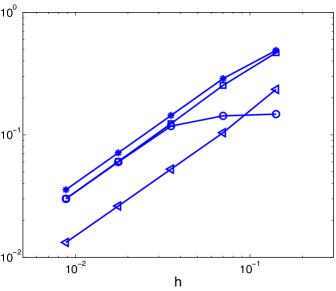
The computation of given by the problem (53) with respect to and to has been performed in [13, Section 4.2] for the following data : , , , . There, it is observed, that for both the BFS and the HCT finite element on regular meshes (non necessarily uniform), the constant behaves like
| (54) |
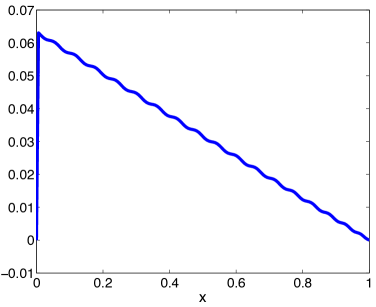
with , a uniformly bounded constant w.r.t. . For the BFS finite element, Table 1 reports some numerical values of while Figure 1 depicts the evolution of w.r.t for and .
Reporting this behavior in the estimate (52), the error behaves like (taking )
The right hand side is minimal for of the order one leading to . This estimate is very likely not optimal but shows the strong convergence of the approximation for regular enough solution. In particular, the estimate (48) of the boundary term by the -norm may result in a loss of precision.
On the other hand, the same argument for the variable indicates, using (45) that the estimate of is
The optimal value for the augmentation parameter is now leading to . Remark that for , the discrete-inf sup constant remains uniformly bounded by below w.r.t. . As observed in [13, Section 4.] (see also the numerical experiments of the present paper), if the influence of the parameter is not really important (for small enough), the choice offers the best rate of convergence.
As discussed and used in [8, Section 4.3], when is approximated with the BFS and HCT finite element, the quantity is asymptotically equivalent w.r.t. to . Therefore, taking in the augmented mixed formulation amounts to relax the constraint in by the weaker one in enough in practice to approximate weak solutions of (1).
4.2 Numerical approximation of the stabilized mixed formulation (17)
We address the numerical approximation of the stabilized mixed formulation (17) with , assuming again that . Let be a real parameter. Let and be two closed finite dimensional spaces such that
The problem (17) becomes : find solution of
| (55) |
In view of the properties of the forms , , and , this formulation is well-posed.
Proceeding as in the proof of [4, Theorem 5.5.2], we first check that the following estimate holds.
Lemma 4.1
Concerning the space , since should belong to , a natural choice is
| (57) |
where is defined by (43). Then, using Lemma 4.1 and the estimate (50), we obtain the following result.
Proposition 4.3 (BFS element for - Rate of convergence for the norm )
Sketch of the proof- The estimate of for any in term of , is detailed in the proof of Proposition 4.2: precisely, we refer to (50). Similarly, we write that, for any ,
| (59) | ||||
for which the estimate follows, in view of the definition of .
In particular, arguing as in the previous section, using Proposition 4.3, the observability estimate () for the variable and the estimate (16) for the variable , we get the following desired global estimate:
Theorem 4.2 (BFS element for - Rate of convergence for the norm)
We emphasize that, within the stabilized formulation, these estimates do not depend of any discrete inf-sup constant. In particular, the positive augmentation parameter can be chosen arbitrarily.
4.3 Numerical approximation of the mixed formulation (28)
We now consider the numerical analysis of the mixed formulation (28) where both the solution and the spatial part of the source are unknown. We take a strictly positive augmentation parameter .
Let and be two finite dimensional spaces parametrized by the variable such that , and for every . Then, we can introduce the following approximated problems: find solution of
| (61) |
Again, for any , the coercivity of the form holds true on the whole space :
so a fortiori, uniformly on the subspace . Therefore, assuming that the discrete inf-sup constant defined by
| (62) |
is, for any , strictly positive, there exists a unique solution of (61) and the following holds true:
Proposition 4.4
Proof- The proof is similar to the proof of Proposition 4.1 using again that and .
The finite dimensional problem (61) reads as follows: find and such that
| (66) |
with matrices similarly defined as in the previous section.
Since the variable is a function of only, we first introduce a triangulation such that and we assume that is a regular family. We denote We then introduce the subspace of defined by
| (67) |
where denotes the space of affine functions in the variable in the element .
Similarly, we define a subdivision of such that and denote . Then, we consider the triangulation defined by such that
Again, we denote by . The triangulation is a regular family for as soon as is a regular family for .
As in the previous section, we now go on in the one dimensional case in space.
4.3.1 -finite elements and order of convergence for
We only discuss the BFS finite element and introduce the space as follows :
| (68) |
with , for all . Finally, we define the space by
so that, for each value of , the variables and share the same triangulation with respect to the variable . We check that for each . In the sequel, for simplicity, we use the notation for .
We then have the following result:
Proposition 4.5 (BFS element for - Rate of convergence for the norm )
We use that, if , , there exists a positive constant such that for any . Consequently, from (47), we have the estimate
This leads to the following estimates :
The proposition then follows from the last two estimates.
It remains now to deduce the convergence of the approximation for a global norm, typically . We write that solves the problem
leading to
On the other hand, proceeding as before, assuming (), we have
leading to
Therefore, in view of Proposition 4.5, we get the following a priori estimate for the -norm :
Theorem 4.3 (BFS element for - Rate of convergence for the -norm)
Remark 7
We have presented along Section 4 error estimates in the one-dimensional case in the case where the space (and for the present section) is based on the BFS finite element. Similar results may be obtained within the HCT finite element. Precisely, we refer to [10, ch. VII, sec. 48, p. 295] where the following interpolation estimates for the HCT element are developed:
for and some constant .
5 Numerical experiments
We now report and discuss some numerical experiments corresponding to mixed formulations (36), (55) and (61) for and respectively.
5.1 Reconstruction of the solution - One dimensional case ()
We take and , , and . We check that for these data, the inequality () holds true. Moreover, in order to check the convergence of the numerical approximations, we consider explicit solutions of (1). We first define the following initial condition in (see [9]):
and . The corresponding solution of (1) is given by
| (71) |
with
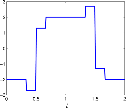
In particular . The corresponding normal derivative is depicted in Figure 2. This example is rather stiff: the normal derivative is in but is discontinuous (in view of the regularity of the initial condition). We compute .
We recall that the direct method amounts to solve, for any , the linear system (42). We use exact integration methods developed in [16] for the evaluation of the coefficients of the matrices. Moreover, the linear system (42) is solved using the LU decomposition method.
We first consider the BFS finite element with uniform triangulation (each element of the triangulation is a rectangle of lengths and so that ). Table 2 collects some numerical values with respect to for and for . We observe the following behavior with respect to :
The evolution of the norm suggests that the unique solution is correctly reconstructed from the observation. Moreover, in agreement with Remark 1, since is by construction the restriction to of the normal derivative of a solution of (1), we check, that the sequence , approximation of , vanishes as . Eventually, in view of the Remark 6, we have , so that approximates correctly the unique corresponding weak solution of (1).
We also check that the minimization of the functional introduced in Proposition 2.3 leads exactly to the same result approximation: we recall that the minimization of the functional corresponds to the resolution of the associated mixed formulation by an iterative Uzawa type method. The minimization is done using a conjugate gradient algorithm (we refer to [13, Section 2.2] for the algorithm). Each iteration amounts to solve a linear system involving the matrix which is sparse, symmetric and positive definite. The Cholesky method is used. The performance of the algorithm depends on the condition number of the operator : precisely, it is known that (see for instance [15]),
where minimizes . denotes the condition number of the operator . As discussed in [13, Section 4.4], the condition number of restricted to (which coincides with the condition number of the matrix ) behaves asymptotically as , where is the constant appearing in (54). This quadratic behavior is the typical one for well-posed elliptic problems. Table 2 reports the number of iterations of the algorithm, initialized with in . We take as a stopping threshold for the algorithm (the algorithm is stopped as soon as the norm of the residue given here by satisfies ). We observe that the number of iterates is sub-linear with respect to , precisely, with respect to the dimension of the approximated problems. This renders this method very attractive from a numerical point of view.
Table 3 reports the results for . We get a slightly better estimate for the norm but slightly worst estimate for the norm . On the other hand, since acts as an augmentation parameter, the convergence of the conjugate gradient algorithm is faster. We also check in view of Remark 6 (specifically, (45) and (54)) that the convergence of toward zero is much lower for than for :
| card() | |||||
|---|---|---|---|---|---|
| CG iterates |
| CG iterates |
|---|
 |
|
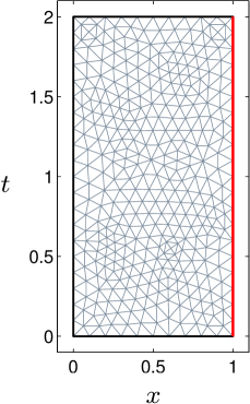
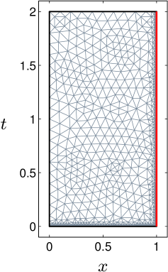
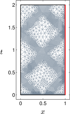
We now discuss the results obtained with the reduced HCT finite element on regular but non-uniform triangulations of the rectangle . Precisely, we consider levels of meshes of described in Table 4. For each of these meshes, we compute as the maximum of the diameters of the triangles composing the triangulation. The coarsest of this meshes is displayed in Figure 2.
| Mesh number | 1 | 2 | 3 | 4 | 5 |
|---|---|---|---|---|---|
| elements | |||||
| points | |||||
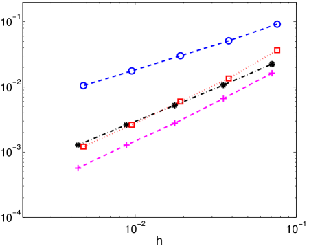
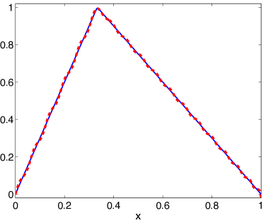
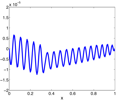
Table 5 collects the numerical results on the reconstruction of the solution from the observation obtained with again . We observe a slightly super linear convergence for the variable and :
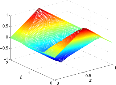
Figure 3 depicts the exact solution computed by (71) and its approximation (computed with the mesh ). Figure 4 represents the relative error reported also in Table 5. Tables 5, 6 and 7 also report the value of the condition number of the matrix . In both situations, as it is usual for elliptic problems, behaves quadratically with respect to .
 |
 |
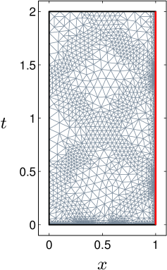
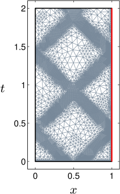
We also emphasize that this variational method which requires a finite element discretization of the time-space is particularly well-adapted to mesh optimization. Still for the example EX1, Figure 5 depicts a sequence of four meshes of : the sequence is initialized with the coarsest mesh described in Table 4 which is locally refined near boundary (where the observation is localized) and near (for a better representation of the initial data). The three other meshes are successively obtained by local refinement based on the norm of the gradient of on each triangle of . As expected, the refinement is concentrated around the lines of singularity of traveling in , generated by the singularity of the initial position . Some information concerning these meshes and the approximation errors obtained where this mesh adaptation strategy is employed are reported in Table 6.
 |
 |
|
 |
 |
| Mesh number | 1 | 2 | 3 | 4 |
|---|---|---|---|---|
| elements | ||||
| points | ||||
We end this section with some numerical results for the stabilized mixed formulation (55). The main difference is that the multiplier is now approximated in a richer space (see (57)) leading to larger linear systems. Table 7 considers the case of the example EX1 with and . In order to compare with the formulation (36), we take again . We observe the convergence w.r.t. and obtain similar rates and constants to the ones in Table 5: in particular, we have
Finally, we also check - in contrast with the mixed formulation (6) - that the positive parameter does not affect the numerical results.
5.2 Reconstruction of the solution - Two dimensional case ()
In this section we illustrate the method introduced in Section 2 on a two-dimensional example. The procedure is similar but a bit more involved on a computational point of view, since is now a subset of . We take again in and in .
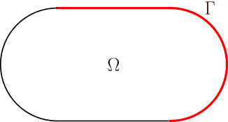
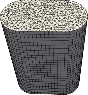
In order to approximate the mixed-formulation (6), we consider a mesh of the domain formed by triangular prisms. This mesh is obtained by extrapolating along the time axis a triangulation of the spatial domain . For all the simulations considered in this section, is the so called Bunimovich’s stadium (see [7]) and . Figure 6-Left displays the domain and the part of the boundary on which the observation is available for while Figure 6-right displays an example of mesh of domain .
|
|
Let be the finite dimensional space defined as follows
| (72) |
is the space of functions corresponding to the reduced Hsieh-Clough-Tocher (HCT) -element recalled in Section 4.1.1; is a space of degree three polynomials on the interval of the form defined uniquely by their value and the value of their first derivative at the point and . In other words, is the finite element space obtained as a tensorial product between the reduced HCT finite element and the cubic Hermite finite element. We check that on each element , the function is determined uniquely in term of the values of at the six nodes of . Therefore, .
We consider meshes formed by triangular prisms of the domain . An example of such a mesh associated to the domain is displayed in Figure 6 right. This mesh is composed by nodes distributed in prismatic elements (this mesh corresponds to the mesh number 2 described in Table 8).
We consider three levels of meshes of the domain formed by the number of prisms and containing the number of nodes reported in Table 8.
| Mesh number | 1 | 2 | 3 |
|---|---|---|---|
| Number of elements | 1 860 | 18 060 | 158 280 |
| Number of nodes | 1 216 | 10 261 | 84 241 |
| (Height of elements) | |||
Comparing to the one dimensional situation described in Section 5.1, the eigenfunctions and eigenvectors of the Dirichlet Laplace operator defined on are not explicitly available. Consequently, from a given set of initial data, we define as the ”exact” solution and note the solution obtained numerically with a very fine discretization, from which we can extract an observation on . Precisely, we solve the hyperbolic equation (1) using a standard time-marching method: we employ a HCT finite elements method in space coupled with a Newmark unconditionally stable scheme for the time discretization.
Here, we solve the hyperbolic equation on the spatial mesh which was extrapolated in time in order to obtain the mesh number 3 of . This two-dimensional mesh contains nodes and triangles and corresponds to the value . As for the time discretization, we use the value . We denote the solution obtained in this way for the initial data given by
| (73) |
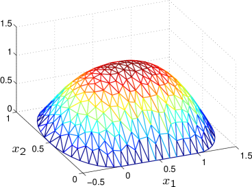
From , we then generate the observation as the restriction of on . The geometry used here allows to compute easily the normal derivative of on the boundary. Finally, from this observation we reconstruct as the solution of the mixed formulation (28) on each of the three meshes described in Table 8. For this simulations we take the augmentation parameter . Table 9 displays some norms of and obtained for the three meshes and illustrates again the convergence of the method.
| Mesh number | 1 | 2 | 3 |
|---|---|---|---|
Figure 7-Left displays the initial position of (73) while Figure 7-Right displays the initial position corresponding to restriction at time of the solution of the inverse problem. Figures correspond to the mesh number 2.. The errors between these two functions are given in the last row of Table 9.
 |
 |
5.3 Reconstruction of the solution and the source - One dimensional case
We now consider the reconstruction of both the state and the source from a partial observation, as discussed in Section 3. In order to construct explicit solution, we first recall that the solution of (1) with zero initial condition can be expanded as follows :
In the following examples, we take defined on , and .
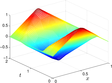
We now report the resolution of the discrete mixed formulation (61). We first consider a rather smooth case, with given by
Table 10 reports the main norms with respect to . Concerning the augmentation parameter , we use which leads to slightly better approximation of the function than . We check the convergence of the approximations as tends to . In particular, we get
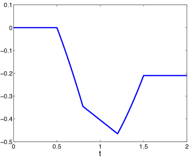
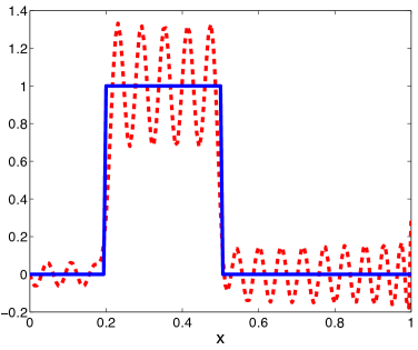
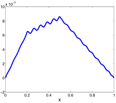
For instance, for (precisely, ) leading to a linear system with unknowns, we get a relative error for of the order of . This allows a very good reconstruction of the corresponding solution . Figure 8-Left depicts the function and its corresponding approximation . Figure 8-Right depicts along the function of magnitude . Here, denotes the Dirichlet Laplacian.
 |
 |
Remarkably, the approach also provides good reconstruction of the solution when the observation is obtained from less regular function. We consider the following rather stiff examples, respectively in and :
The corresponding normal derivatives in (see [27]) and in respectively, are depicted on Figure 9.
 |
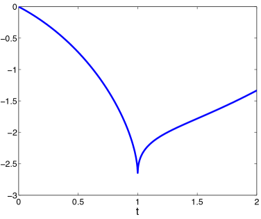 |
Table 11 reports some norms with respect to for the example (EX4). We observe the convergence as with as expected a lower rate : precisely, we compute
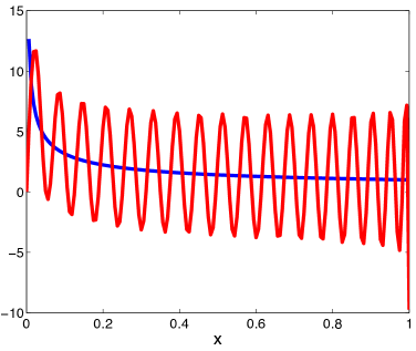
For , Figure 11 depicts the functions and leading to a relative error equal to . The approximation oscillates around and suggests that the convergence (in agreement with Theorem 3.1) may not hold pointwise but in a weaker (average) sense. Again, this weak convergence of the source term is enough to reconstruct with robustness the solution . The function of magnitude suggests the efficiency of the method to reconstruct the spatial term of the source .
 |
 |
 |
 |
6 Concluding remarks and perspectives
The mixed formulations we have introduced here in order to address inverse problems for hyperbolic equations seems original. These formulations are nothing else than the Euler systems associated to least-squares type functionals and depend on both the state to be reconstruct and a Lagrange multiplier. This Lagrange multiplier is introduced to take into account the state constraint and turns out to be the controlled solution of a hyperbolic equation with the source term . This approach, recently used in a controllability context in [13], leads to a variational problem defined over time-space functional Hilbert spaces, without distinction between the time and the space variable. The main ingredients are, first a unique continuation type property for the hyperbolic equation (assuming some geometric conditions on the measurement zone) allowing to prove the well-posedness of the mixed formulation, and second, a (strong) generalized observability inequality, allowing to quantify the global reconstruction of the solution.
At the practical level, the discrete mixed time-space formulation is solved in a systematic way in the framework of the finite element theory. The approximation is conformal allowing to obtain the strong convergence of the approximation as the discretization parameters tends to zero. In particular, we emphasize that there is no need, contrarily to the classical approach, to prove some uniform discrete observability inequality: we simply use the observability inequality on the finite dimensional discrete space. The resolution amounts to solve a sparse symmetric linear system : the corresponding matrix can be preconditioned if necessary, and may be computed once for all as it does not depend on the observation . Eventually, the space-time discretization of the domain allows an adaptation of the mesh so as to reduce the computational cost and capture the main features of the solutions. Similarly, this space-time formulation is very appropriate to the non-cylindrical situation.
In agreement with the theoretical convergence, the numerical experiments reported here display a very good behavior and robustness of the approach: the reconstructed approximate solution converges strongly to the solution of the hyperbolic equation associated to the available observation. Remark that from the continuous dependence of the solution with respect to the observation, the method is robust with respect to the possible noise on the data.
Eventually, since the mixed formulations rely essentially on a generalized observability inequality, it may be employed to any other observable systems for which such property is available : we mention notably the parabolic case usually badly conditioned – in view of regularization property – and for which direct and robust methods are certainly very advantageous. This is in contrast with the Luenberger approach (mentioned in the introduction) which assume the reversibility in time of the equation We also mention that this kind of approach may be used to reconstruct potential and coefficient.
References
- [1] C. Bardos, G. Lebeau, and J. Rauch, Sharp sufficient conditions for the observation, control, and stabilization of waves from the boundary, SIAM J. Control Optim., 30 (1992), pp. 1024–1065.
- [2] L. Beilina and M. V. Klibanov, Approximate Global Convergence and Adaptivity for coefficient inverse problems, Springer US, 2012.
- [3] M. Bernadou and K. Hassan, Basis functions for general Hsieh-Clough-Tocher triangles, complete or reduced, Internat. J. Numer. Methods Engrg., 17 (1981), pp. 784–789.
- [4] D. Boffi, F. Brezzi, and M. Fortin, Mixed finite element methods and applications, vol. 44 of Springer Series in Computational Mathematics, Springer, Heidelberg, 2013.
- [5] L. Bourgeois and J. Dardé, A duality-based method of quasi-reversibility to solve the Cauchy problem in the presence of noisy data, Inverse Problems, 26 (2010), pp. 095016, 21.
- [6] L. Bourgeois and J. Dardé, A quasi-reversibility approach to solve the inverse obstacle problem, Inverse Probl. Imaging, 4 (2010), pp. 351–377.
- [7] L. A. Bunimovich, On the ergodic properties of nowhere dispersing billiards, Comm. Math. Phys., 65 (1979), pp. 295–312.
- [8] C. Castro, N. Cîndea, and A. Münch, Controllability of the linear one-dimensional wave equation with inner moving forces, SIAM J. Control Optim., 52 (2014), pp. 4027–4056.
- [9] D. Chapelle, N. Cîndea, and P. Moireau, Improving convergence in numerical analysis using observers—the wave-like equation case, Math. Models Methods Appl. Sci., 22 (2012), pp. 1250040, 35.
- [10] P. G. Ciarlet, The finite element method for elliptic problems, vol. 40 of Classics in Applied Mathematics, Society for Industrial and Applied Mathematics (SIAM), Philadelphia, PA, 2002. Reprint of the 1978 original [North-Holland, Amsterdam; MR0520174 (58 #25001)].
- [11] N. Cîndea, E. Fernández-Cara, and A. Münch, Numerical controllability of the wave equation through primal methods and carleman estimates, ESAIM Control Optim. Calc. Var., 19 (2013), pp. 1076–1108.
- [12] N. Cîndea and A. Münch, Inverse problems for linear hyperbolic equations using mixed formulations, To appear in Inverse Problems (http://arxiv.org/abs/1502.00114).
- [13] , A mixed formulation for the direct approximation of the control of minimal -norm for linear type wave equations, Calcolo, 52 (2015), pp. 1–44.
- [14] C. Clason and M. V. Klibanov, The quasi-reversibility method for thermoacoustic tomography in a heterogeneous medium, SIAM J. Sci. Comput., 30 (2007/08), pp. 1–23.
- [15] J. W. Daniel, The approximate minimization of functionals, Prentice-Hall Inc., Englewood Cliffs, N.J., 1971.
- [16] D. A. Dunavant, High degree efficient symmetrical Gaussian quadrature rules for the triangle, Internat. J. Numer. Methods Engrg., 21 (1985), pp. 1129–1148.
- [17] M. Fortin and R. Glowinski, Augmented Lagrangian methods, vol. 15 of Studies in Mathematics and its Applications, North-Holland Publishing Co., Amsterdam, 1983. Applications to the numerical solution of boundary value problems, Translated from the French by B. Hunt and D. C. Spicer.
- [18] R. Glowinski, J.-L. Lions, and J. He, Exact and approximate controllability for distributed parameter systems, vol. 117 of Encyclopedia of Mathematics and its Applications, Cambridge University Press, Cambridge, 2008. A numerical approach.
- [19] M. V. Klibanov and A. Timonov, Carleman estimates for coefficient inverse problems and numerical applications, Inverse and Ill-posed Problems Series, VSP, Utrecht, 2004.
- [20] V. Komornik and P. Loreti, Observability of discretized wave equations, Bol. Soc. Parana. Mat. (3), 25 (2007), pp. 67–76.
- [21] J.-L. Lions, Contrôlabilité exacte, perturbations et stabilisation de systèmes distribués. Tome 1, vol. 8 of Recherches en Mathématiques Appliquées [Research in Applied Mathematics], Masson, Paris, 1988. Contrôlabilité exacte. [Exact controllability], With appendices by E. Zuazua, C. Bardos, G. Lebeau and J. Rauch.
- [22] J.-L. Lions and E. Magenes, Non-homogeneous boundary value problems and applications. Vol. I, Springer-Verlag, New York-Heidelberg, 1972. Translated from the French by P. Kenneth, Die Grundlehren der mathematischen Wissenschaften, Band 181.
- [23] A. Meyer, A simplified calculation of reduced hct-basis functions in a finite element context, Comput. Methods Appl. Math., 12 (2012), pp. 486–499.
- [24] A. Münch, A uniformly controllable and implicit scheme for the 1-D wave equation, M2AN Math. Model. Numer. Anal., 39 (2005), pp. 377–418.
- [25] K. Ramdani, M. Tucsnak, and G. Weiss, Recovering and initial state of an infinite-dimensional system using observers, Automatica J. IFAC, 46 (2010), pp. 1616–1625.
- [26] M. Yamamoto, Stability, reconstruction formula and regularization for an inverse source hyperbolic problem by a control method, Inverse Problems, 11 (1995), pp. 481–496.
- [27] M. Yamamoto and X. Zhang, Global uniqueness and stability for an inverse wave source problem for less regular data, J. Math. Anal. Appl., 263 (2001), pp. 479–500.