Approximate hedging problem with transaction costs in stochastic volatility markets††thanks: The second author is partially supported by Russian Science Foundation (research project No. 14-49-00079) and by the National Research Tomsk State University.
Abstract
This paper studies the problem of option replication in general stochastic volatility markets with transaction costs, using a new specification for the volatility adjustment in Leland’s algorithm [23]. We prove several limit theorems for the normalized replication error of Leland’s strategy, as well as that of the strategy suggested by Lépinette [27]. The asymptotic results obtained not only generalize the existing results, but also enable us to fix the under-hedging property pointed out by Kabanov and Safarian in [18]. We also discuss possible methods to improve the convergence rate and to reduce the option price inclusive of transaction costs.
Keywords: Leland strategy, transaction costs, stochastic volatility, quantile hedging, approximate hedging, high frequency markets
Mathematics Subject Classification (2010): 91G20; 60G44; 60H07
JEL Classification G11; G13
1 Introduction
Leland [23] suggests a simple method for pricing standard European options in markets with proportional transaction costs. He argues that transaction costs can be accounted for in the option price by increasing the volatility parameter in the classical Black-Scholes model [4]. Leland then claims, without giving a mathematically rigorous proof, that the replicating portfolio of the corresponding discrete delta strategy converges to the option payoff as the number of revisions goes to infinity, if the transaction cost rate is a constant independent of , or decreases to zero at the rate . The latter statement is proved by Lott in his PhD thesis [30]. In fact, this property still holds if the transaction cost coefficient converges to zero at any power rate [18].
However, a careful analysis shows that the replicating portfolio does not converge to the option payoff when the cost rate is a constant independent of . Kabanov and Safarian [18] find an explicit limit for the hedging error, which is negative, showing that the replication problem is not completely solved in Leland’s framework. Pergamenshchikov [34] obtains a weak convergence for the normalized hedging error and points out that, for the case of constant transaction cost, the rate of convergence in Kabanov-Safarian’s result is . This limit theorem is of practical importance because it provides the asymptotic distribution of the hedging error. Note that the rate of convergence can be improved using non-uniform revisions [27, 9]. In these papers, Lépinette and his co-authors suggest a modification to Leland’s strategy to solve the discrepancy identified by Kabanov and Safarian. For a recent account of the theory, we refer the reader to Section 2 and [18, 24, 26, 27, 13, 14, 9, 34].
In this study, we examine the problem of approximate hedging of European style options in stochastic volatility (SV) markets with constant transaction costs (the reader is referred to e.g. [11] and the references therein for motivations and detailed discussions related to SV models). In particular, we establish a weak convergence for the normalized hedging error of Leland’s strategy using a simple volatility adjustment, in a general SV setting. The results obtained not only generalize the existing results, but also provide a method for improving the rate of convergence. Furthermore, it turns out that superhedging can be attained by controlling a model parameter.
Let us emphasize that the classic form for adjusted volatility proposed in [23] and applied in [18, 19, 24, 25, 27] may not be applicable in SV models. The reason is that option pricing and hedging are intrinsically different in SV markets than in the classical Black-Scholes framework. In particular, the option price now depends on future realizations of the volatility process. In general, this information may not be statistically available for all investors. To treat this issue, we suggest a new specification for adjusted volatility in Leland’s algorithm. Although we employ an artificially modified volatility, simpler than the well-known version used in the previous literature, the same asymptotic results are obtained for SV contexts. In addition, the rate of convergence can be improved by controlling a model parameter. Note that, in the above-mentioned papers, approximation procedures are mainly based on moment estimates. This essential technique no longer works in general SV models, unless some intrinsic conditions are imposed on the model parameters [2, 28]. It is useful to remember that our goal is to establish a weak convergence for the normalized replicating error which only requires convergence in probability of the approximation terms. Thus, in the approximation procedure, the integrability issue can be avoided in order to keep our model setting as general as possible.
As discussed in [34], the option price (inclusive of transaction costs) in Leland’s algorithm may be high (it, in fact, approaches the buy-and-hold price), even for small values of the revision number. Another practical advantage of our method is that the option price can be reduced as long as the option seller is willing to take a risk in option replication. This approach is inspired by the theory of quantile hedging [10].
The remainder of the paper is organized as follows. In Section 2, we give a brief review of Leland’s approach. Section 3 is devoted to formulating the problem and presenting our main results. Section 4 presents some direct applications to pricing and hedging. Section 5 discusses common SV models that fulfill our condition on the volatility function. A numerical result for Hull-White’s model is also provided for illustration. Section 6 connects our results to high-frequency markets with proportional transaction costs. The proofs of our main results are reported in Section 7. Auxiliary lemmas can be found in the Appendix.
2 Approximate hedging with transaction costs: A review of Leland’s approach
In a complete no-arbitrage model (i.e., there exists a unique equivalent martingale measure under which the stock price is a martingale), options can be completely replicated by a self-financing trading strategy. The option price, defined as the replication cost, is the initial capital that the investor must invest to obtain a complete hedge. In fact, the option price can be computed as the expectation of the discounted claim under the unique equivalent martingale measure. This principle plays a central role in the well-known Black-Scholes model. For simplicity, let us consider a continuous time model of a two-asset financial market on the time interval , where the bond price is equal to 1 at all times. The stock price dynamics follow the stochastic differential equation
| (1) |
where and are positive constants and is a standard Wiener process. As usual, let . We recall that a financial strategy is an admissible self-financing strategy if it is bounded from below, - adapted with a.s., and the portfolio value satisfies
The classic hedging problem is to find an admissible self-financing strategy whose terminal portfolio value exceeds the payoff , or
where is the strike price. The standard pricing principle shows that the option price is given by the well-known formula [4]
| (2) |
where
| (3) |
Here, is the standard normal distribution function. In the following, we denote by the density: . One can check directly that
| (4) |
By assuming that continuous portfolio adjustments are possible with zero transaction costs, Black and Scholes [4] argue that the option payoff can be dynamically replicated using the delta strategy (i.e., the partial derivative of the option price with respect to the stock price).
It is clear that the assumption of continuous portfolio revision is not realistic. Moreover, continuous trading would be ruinously expensive in the case of nonzero constant proportional transaction costs because the delta strategy has infinite variation. This simple intuition contradicts the argument of Black and Scholes that, if trading takes places reasonably frequently, then hedging errors are relatively small. Therefore, option pricing and replication with nonzero trading costs are intrinsically different from those in the Black-Scholes setting. Note that it may be very costly to assure a given degree of accuracy in replication with transaction costs. In what follow, we show that Leland’s increasing volatility principle [23] is practically helpful in such contexts.
2.1 Constant volatility case
Leland’s approach [23] provides an efficient technique to deal with transaction costs. This method is simply based on the intuition that transaction costs can be accounted for in the option price as a reasonable extra fee, necessary for the option seller to cover the option return. It means that in the presence of transaction costs, the option becomes more expensive than in the classic Black-Scholes framework. This is intuitively equivalent to an increase in the volatility parameter in the Black-Scholes formula. Let us shortly describe Leland’s approach [23, 18]. Suppose that for each trading activity, the investor has to pay a fee directly proportional to the trading volume, measured in dollar value. Assume that the transaction cost rate is given by the law , where is the number of revisions. Here, and are two fixed parameters. The basic idea of Leland’s method is to replace the true volatility parameter in the Black-Scholes model by , artificially modified as
| (5) |
In this case, the option price is given by , the Black-Scholes’s formula. For the problem of option replication, Leland suggests the following discrete strategy, known as Leland’s strategy,
| (6) |
Here, the number of shares held in the interval is the delta strategy calculated at the left bound of this interval. Then, the replicating portfolio value takes the form
| (7) |
where the total trading volume is (measured in dollar value). Recall that the option price is the solution of the Black-Scholes PDE with the adjusted volatility
| (8) |
Using Itô’s formula, we can represent the tracking error, , as
| (9) |
Remark 1 (Leland).
The specific form (5) results from the following intuition: the Lebesgue integral in (9) is clearly well approximated by the Riemann sum of the terms , while can be replaced by
because . Hence, it is reasonable to expect that the modified volatility defined in (5) will give an appropriate approximation to compensate transaction costs.
Leland [23] conjectures that the replication error converges in probability to zero as for the case of constant proportional transaction cost (i.e., ). He also suggests, without giving a rigorous proof, that this property is also true for the case . In fact, Leland’s second conjecture for is correct and is proved by Lott in his PhD thesis [30].
Theorem 2.1 (Leland-Lott [23, 30]).
For , strategy (6) defines an approximately replicating portfolio as the number of revision intervals tends to infinity
This result is then extended by Ahn et al. in [1] to general diffusion models. Kabanov and Safarian [18] observe that the Leland-Lott theorem remains true as long as the cost rate converges to zero as .
Theorem 2.2 (Kabanov-Safarian [18]).
For any ,
In [26, 19], the authors study the Leland-Lott approximation in the sense of convergence for the case .111 Seemingly, mean-square replication may not contain much useful information because gains and losses have different meaning in practice. Clearly, if the modified volatility is independent of .
Theorem 2.3 (Kabanov-Lépinette [26]).
Let . The mean-square approximation error of Leland’s strategy, with defined in (5), satisfies the following asymptotic equality
where is some positive function.
Theorem 2.3 suggests that the normalized replication error converges in law as .
Theorem 2.4 (Lépinette-Kabanov [19]).
For , the processes converge weakly in the Skorokhod space to the distribution of the process , where is an independent Wiener process.
Remark 2.
An interesting connection between this case and the problem of hedging under proportional transaction costs in high-frequency markets is discussed in Section 6.
It is important to note that Leland’s approximation in Remark 1 is not mathematically correct and thus, his first conjecture is not valid for the case of constant transaction costs. In fact, as , the trading volume can be approximated by the following sum (which converges in probability to defined in (11))
where and
| (10) |
A careful study confirms that there is a non trivial discrepancy between the limit of the replicating portfolio and the payoff for the case .
Theorem 2.5 (Kabanov-Safarian [18]).
For , converges to in probability, where
| (11) |
with and independent of .
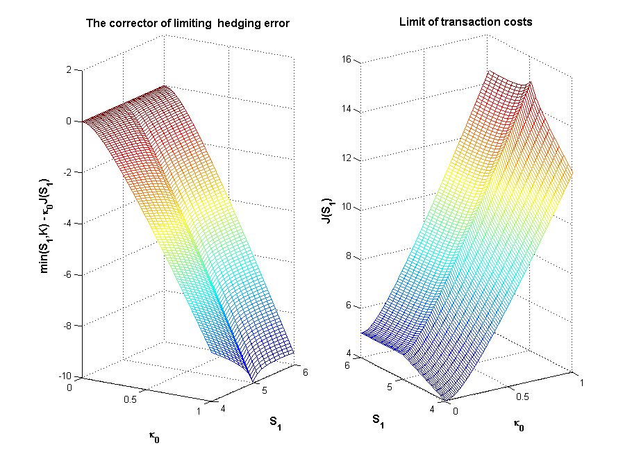
Under-hedging: It is important to observe that the problem of option replication is not completely solved in the case of constant transaction costs. Indeed, considering that and the identity
| (12) |
we obtain (for the parameter given in (5)) that equals Now, Anderson’s inequality (see, for example [17], page 155) implies directly that for any , Therefore, thus, the option is asymptotically under-hedged in this case.
In approximation procedures, one should also pay attention to the fact that and its derivatives depend on the number of revisions when . In addition, the coefficient appearing in (5) can be chosen in an arbitrary way. Pergamenshchikov [34] shows that the rate of convergence in Kabanov-Safarian’s theorem is and provides a weak convergence for the normalized replication error.
Theorem 2.6 (Pergamenshchikov [34]).
Theorem 2.6 is of practical importance because it not only gives the asymptotic information about the hedging error, but also provides a reasonable way to fix the under-hedging issue (see Section 4). Darses and Lépinette [9] modify Leland’s strategy in order to improve the convergence rate in Theorem 2.6 by applying a non-uniform revision policy , defined by
| (14) |
The adjusted volatility is then taken as where is the inverse function of . Furthermore, the discrepancy in Theorems 2.5 and 2.6 can be removed by employing the following modified strategy, known as Lépinette’s strategy [27],
| (15) |
Theorem 2.7.
Let be the terminal value of the strategy (15) with . Then, for any , the sequence weakly converges to a centered mixed Gaussian variable as , where
| (16) |
2.2 Time-dependent volatility case
Assume now that is a positive non-random function and the payoff is a continuous function with continuous derivatives, except at a finite number of points. Under the non-uniform rebalancing plan (14), the enlarged volatility should take the form
| (17) |
Theorem 2.8 (Lépinette [24]).
Let be a strictly positive Lipschitz and bounded function. Moreover, suppose that is a piecewise twice differentiable function and there exist and , such that . Then, for any , the replicating portfolio of Leland’s strategy converges in probability to the payoff as . Moreover, for ,
where and are positive functions that depend on the payoff .
2.3 Discussion
From Remark 1, the modified volatility defined by (5) would seem to give an appropriate approximation that accounts for transaction costs. However, this is not always the case because the option price inclusive of transaction costs now depends on the rebalancing number. In more general models, this specific choice may generate technical issues. For example, in local volatility models [24], proving the existence of the solution to (8) requires patience and effort, because depends on the stock price. On the other hand, it is interesting to observe that the true volatility plays no role in the approximation procedure from a mathematical point of view. In fact, all the results for the case can be obtained by using the form , where the first term has been removed. More generally, we can take the following form
| (18) |
for some positive constant , which will be specified later. Of course, the limiting value of transaction costs will change slightly. Let us emphasize that using the simple form (18) is important for two reasons. First, it allows us to carry out a far simpler approximation than is used in the existing literature. Second, Leland’s strategy with defined in (5) may no longer work in stochastic volatility (SV) markets. Indeed, in those markets, option prices depend on future volatility realizations, which are not statistically available. We show in the remainder of the paper, that the simple form (18) (a deterministic function of ) is helpful for approximate hedging in a very general SV setting. It should be noted that the approximation methodology developed here still works well for the classical form (5), if the volatility risk premium depends only on the current value of the volatility process [36, 37].
We conclude the section by mentioning that Leland’s algorithm is of practical importance due to its ease of implementation. The case of constant transaction costs should be investigated in more general situations, for instance, where volatility depends on external random factors, or jumps in stock prices are considered.
3 Model and main results
Let be a standard filtered probability space with two standard independent adapted Wiener processes and , taking their values in . Our financial market consists of one risky asset governed by the following equations on the time interval
| (19) |
where is the correlation coefficient. It is well known in the literature of SDEs that if and are measurable in , linearly bounded and locally Lipschitz, there exists a unique solution to the last equation of system (19). For this fundamental result, see Theorem 5.1 and [12, 29]. For simplicity, assume that the interest rate equals zero. Thus , the non-risky asset is chosen as the numéraire.
In this section, we consider the problem of approximate hedging with constant proportional costs using the principle of increasing volatility for model (19). As discussed in Subsection 2.3, the adjusted volatility is chosen as
| (20) |
The replicating portfolio is revised at , as defined by (14). The parameter plays an important role in controlling the rate of convergence and is specified later. As shown below, the limiting value of the total trading volume is essentially related to the dependence of on the number of revisions.
Remark 4.
Intuitively, using an independent adjusted volatility seems unnatural because it fails to account for market information. However, the techniques developed in this note are well adapted to the case where the adjusted volatility depends on a volatility process driven by an independent Brownian motion. In such a context, if the volatility risk premium depends only on the current volatility process, then the no-arbitrage option price (without transaction costs) is the average of the Black-Scholes prices over the future paths of the volatility process [36, 37].
Recall that is the solution of the Cauchy problem (8) with two first derivatives, as described in (4): and where
| (21) |
Remark 5.
We make use of the following condition on the volatility function.
Assume that is a function and there exists such that
Assumption is not restrictive and is fulfilled in many popular SV models (see Section 5 and [35]).
3.1 Asymptotic results for Leland’s strategy
Let us study the replication error for Leland’s strategy defined in (6). The replicating portfolio is defined by (7). Now, by Itô’s formula,
| (22) |
where . Setting , we can represent the replication error as
| (23) |
where and is defined as in (7).
Let us first emphasize that complete replication in SV models is far from obvious. In our setting, converges to zero faster than , with defined as in (16). The gamma error approaches at the same rate. On the other hand, the total trading volume converges in probability to the random variable , defined by
| (24) |
where independent of and . Our goal is to study the convergence of the normalized replication error corrected by these explicit limiting values, by applying the theory of limit theorems for martingales [15]. To do so, we search for the martingale part in the approximation of the above terms by developing a special discretization procedure in Section 7.
Theorem 3.1.
Suppose that condition holds and is a fixed positive constant. Then,
weakly converges to a centered mixed Gaussian variable as .
Remark 6.
Remark 7.
Note that , where is the payoff of a classical European call option. Then, from Theorem 3.1, the wealth process approaches as . This can be explained by the fact that the option is now sold at a higher price because as In other words, Leland’s strategy now converges to the well-known buy-and-hold strategy [22]: buy a stock share at time for price and keep it until expiry.
We now present a method for improving the rate of convergence in Theorem 3.1. To this end, by letting , we observe that
| (25) |
which is independent of . This suggests that the rate of convergence in Theorem 3.1 can be improved if is taken as a function of . Our next result is established under the following condition on .
The parameter is a function of such that
Theorem 3.2.
Under conditions ,
weakly converges to a centered mixed Gaussian variable as .
3.2 Asymptotic result for Lépinette’s strategy
Let us study the replication error of Lépinette’s strategy , as defined in (15). As before, the replicating portfolio is where
| (26) |
Now, by Itô’s formula, the tracking error is
| (27) |
where . Then, we have the following strengthening of Theorem 2.7.
Theorem 3.3.
Suppose that is fulfilled. Then, for any , the sequence
weakly converges to a centered mixed Gaussian variable as .
Remark 9.
Theorem 2.7 can be established from Theorem 3.3 with when the volatility is a constant. In addition, in our model, the parameter takes its values in the interval , which is slightly more general than the condition imposed in Theorem 2.7. Moreover, if the classical form of adjusted volatility is applied for Lépinette’s strategy, then complete replication can be reached by taking , and we again have the result established in [9].
Corollary 3.1.
Under conditions , the wealth sequence converges in probability to .
Note that we do not obtain an improved convergence version of Theorem 3.3 because converges to zero at the order of .
4 Application to the pricing problem
In this section, we present an application to the problem of option pricing with transaction costs. We first emphasize that it is impossible to obtain a non-trivial perfect hedge in the presence of transaction costs, even in constant volatility models. In fact, the seller can take the buy-and-hold strategy, but this leads to a high option price. We show below that the price can be reduced in certain ways so that the payoff is covered with a given probability.
4.1 Super-hedging with transaction costs
To be on the safe side, the investor searches for strategies with terminal values greater than the payoff. Such strategies are solutions to dynamic optimization problems. More precisely, let be a general contingent claim and let and be the set of all admissible strategies with initial capital and the terminal value of strategy , respectively. Then, the super-replication cost for is determined as
| (28) |
(see [22] and the references therein for more details). In the presence of transaction costs, Cvitanić and Karatzas [8] show that the buy-and-hold strategy is the unique choice for super-replication, and then is the super-replication price. In this section, we show that this property still holds for approximate super-hedging. The following observation is a direct consequence of Theorem 3.2 when is a function of .
Proposition 4.1.
Under conditions , . The same property holds for Lépinette’s strategy.
4.2 Asymptotic quantile pricing
As seen ealier, super-hedging in the presence of transaction costs leads to a high option price. Practically, one can ask by how much the initial capital can be reduced in exchange for a shortfall probability at the terminal moment. More precisely, for a given significance level , the seller may look for hedges with a minimal initial cost
This construction is motivated by quantile hedging theory, which goes back to [10, 33]. For related discussions, we refer to [10, 33, 34, 5, 7, 6]. Here, we adapt this idea to the hedging problem. Recall that the super-hedging price of Leland’s algorithm is . On the seller’s side, we propose a price for the option, for a properly chosen . We then follow Leland’s strategy for replication. To be safe at the terminal moment, we need to choose such that the probability of the terminal portfolio exceeding the sum of the real objective (i.e., the payoff) and the additional amount is greater than . Here, is a significance level predetermined by the seller. By Proposition 4.1, this goal can be achieved for sufficiently large . To determine the option price, it now remains to choose the smallest value of . Motivated by (29), we define this by
| (30) |
Thus, the reduction in the option price is given by . Clearly, smaller values of yield cheaper options.
Next, we show that the option price is significantly reduced, compared with powers of the parameter .
Proof.
We first observe that and tends to as . Set . Then, for sufficiently small such that , one has
Therefore,
| (32) |
where and . To estimate this probability, we note that for any integer , (see [29, Lemma 4.11, p.130]). Set . For any ,
Therefore, for sufficiently small , we have
Then, , where . Letting , we get , which implies (31). ∎
The boundedness of the volatility function is essential for the above comparison result. If we wish to relax this assumption, the price reduction will be smaller than that in Proposition 4.2.
Proposition 4.3.
Suppose that , for some constant . Then, for ,
| (33) |
Proof.
For any positive constant we set
| (34) |
which is understood to be the first time that the log-price’s variance passes level . Then, from (32),
| (35) |
where , , and . Note that for any , the stopped process is a martingale and . Therefore, the first probability on the right side of (35) can be estimated as
where . By the hypothesis and Chebysev’s inequality, we have
Hence, By choosing and letting , one deduces that for any and for some positive constant ,
Note that . Then, including in the last inequality we obtain property (33). ∎
5 Examples and numerical results
In this section, we list some well-known SV models for which condition is fulfilled. To this end, we need some moment estimates for solutions to general SDEs,
| (36) |
where is a standard Wiener process and are two smooth functions. We first recall the well-known result in SDE theory (see for example [12, Theorem 2.3, p.107]).
Theorem 5.1.
Suppose that and are measurable in , linearly bounded and locally Lipschitz. If for some integer , then there exists a unique solution to (36) and
where are positive constants dependent on .
In the context of Theorem 5.1, condition holds if the volatility function and its derivative have polynomial growth , for some positive constant and .
Hull-White models: Assume that follows a geometric Brownian motion
| (37) |
where , and are some constants, and is a standard Brownian motion correlated with . Put . Then, by Theorem 5.1, we have
as long as . Therefore, condition is fulfilled in (37).
Uniform elliptic volatility models: Suppose that volatility is driven by a mean-reverting Orstein-Uhlenbeck process
| (38) |
In this case, . Thus, condition is verified throughout Theorem 5.1.
Heston models: Heston [16] proposes a SV model where volatility is driven by a CIR process, which also known as a square root process. This model can be used in our context. Indeed, assume now that the price dynamics are given by the following:
| (40) |
For any and , the last equation admits a unique strong solution . Note that the Lipschitz condition in Theorem 5.1 is violated, but by using the stopping times technique, we can directly show that . Hence, this implies that condition is satisfied for model (40).
Similarly, we can check that also holds for Ball-Roma models [3] or, more generally, for a class of processes with bounded diffusion satisfying the following condition.
There exist positive constants and such that
Proposition 5.1.
Under condition , there exists such that .
Proof.
The proof uses the same method as in Proposition 1.1.2 in [20]. ∎
Scott models: Suppose that volatility follows an Orstein-Uhlenbeck, as in Stein-Stein models, and the function takes the exponential form
| (41) |
where and are constants. Here, is chosen such that , defined as in Proposition 5.1. Clearly, and condition is fulfilled because
Numerical result for the Hull-White model: We provide a numerical example for the approximation result of Lépinette’s strategy in the Hull-White model (37). By Theorem 3.3, the corrected replication error is given by , where .
| gain/loss | corrected error | lower bound | upper bound | price | strategy | |
|---|---|---|---|---|---|---|
| 10 | 0.1523845 | -0.2225988 | -0.2363122 | -0.2088854 | 0.7914033 | 0.9013901 |
| 50 | 0.2966983 | -0.0596194 | -0.0670452 | -0.0521936 | 0.9399330 | 0.9706068 |
| 100 | 0.3086120 | -0.0288526 | -0.0350141 | -0.0226911 | 0.9746527 | 0.9875094 |
| 500 | 0.2955755 | 0.0032387 | -0.0005821 | 0.0070594 | 0.9991733 | 0.9995891 |
| 1000 | 0.2851002 | 0.0012409 | -0.0021596 | 0.0046415 | 0.9999300 | 0.9999652 |
| gain/loss | corrected error | lower bound | upper bound | price | strategy | |
| 10 | 0.2859197 | -0.0744180 | -0.0813544 | -0.0674816 | 0.9246420 | 0.9659700 |
| 50 | 0.3172523 | -0.0069238 | -0.0115426 | -0.0023049 | 0.9921661 | 0.9962377 |
| 100 | 0.3033519 | 0.0007474 | -0.0030916 | 0.0045864 | 0.9984346 | 0.9992385 |
| 500 | 0.3618707 | 0.0001296 | -0.0024741 | 0.0027333 | 0.9999977 | 0.9999989 |
| 1000 | 0.3334375 | 0.0003996 | -0.0020559 | 0.0028550 | 1 | 1 |
The difference can be seen as the gain/loss of strategy . For a numerical evaluation, we simulate trajectories in a crude Monte-Carlo method, where the correlation coefficient of the two Brownian motions is and the other initial values are , and . For each value of , we estimate the average value of the corrected error and give the corresponding intervals defined by lower and upper bounds. Initial numbers of shares held are given in the last column of Tables 1 and 2. It turns out that strategy converges to the buy-and-hold strategy and the option prices approach the super-hedging price . We also see that the convergence of the corrected replication error to zero is somehow slow. In fact, increasing values of can provide a faster convergence, but this unexpectedly leads to super-replication more rapidly.
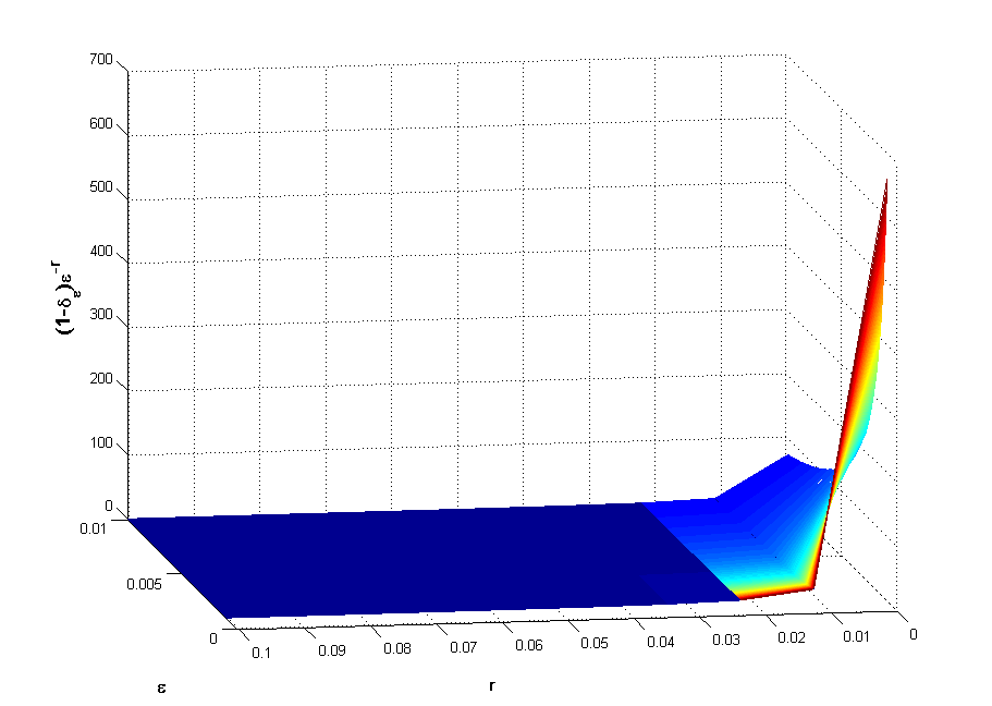
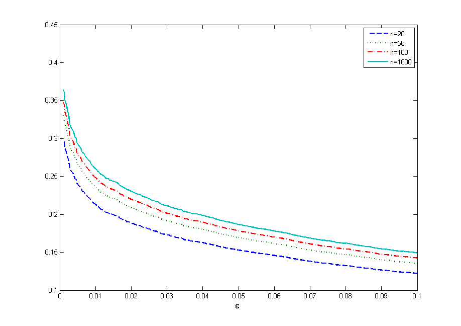
We now provide a numerical illustration for the quantile hedging result of Proposition 4.2. For simplicity, suppose that and that follows a geometric Brownian motion as above. To compare the reduction factor with powers of significance level , we compute for and , with . Then, (31) is confirmed by the simulation result (see Figure 2(a)). The simulation also shows that the option price inclusive of transaction costs is , which is cheaper than the super-hedging price , for a shortfall probability less than . Of course, it is reasonable to replace by the option price inclusive of transaction costs . The simulated reduction in the option price is then given in Figure 2(b).
6 High-frequency markets
We now assume that purchases of the risky asset are carried out at a higher ask price , whereas sales earn a lower bid price . Here the mid-price is given as in model (19) and is the halfwidth of the bid-ask spread. Then, for any trading strategy of finite variation , the wealth process can be determined by
| (42) |
where is the total variation of . Observe that the first two terms are the classic components in frictionless frameworks, and respectively describe the initial capital and gains from trading. The last integral in (42) accounts for transaction costs incurred from the trading activities by weighting the total variation222It is important to know that the classical Black-Scholes strategy is not finite variation. of the strategy with the halfwidth of the spread.
For optimal investment and consumption with small transaction costs [21], the additional terms should be added in the formulation of . In such cases, approximate solutions are usually determined through an asymptotic expansion around zero of the halfwidth spread , where the leading corrections are obtained by collecting the inputs from the frictionless problem.
In this section, we are only interested in replication using discrete strategies in Leland’s spirit. Assume that for replication, the option seller applies a discrete hedging strategy , revised at dates defined by as in Section 3. The corresponding wealth process is now given by
| (43) |
To treat the risk of transaction costs, we again apply the increasing volatility principle. Note that in high frequency markets, the bid-ask spread is, in general, of the same order of magnitude as price jumps333We thank an anonymous referee for pointing out the correspondence of the case to this setting. . Hence, should be of the form for some positive constant . Then, this case corresponds to the Leland-Lott framework with .
In our context, the method in Section 3 is still helpful when is replaced by Leland’s or Lépinette’s strategy.
Proposition 6.1.
Let , and assume that the adjusted volatility is of the form as in (20). For both Leland’s and Lépinette’s strategies, the sequence of replicating portfolio values converges in probability to . In particular, converges to a mixed Gaussian variable as .
Proof.
The proof is a direct consequence of Theorem 3.1, because the total transaction cost now converges to zero. ∎
Note that the case studied in Section 3 corresponds to the assumption , for some constant . This specific form means that the market is more illiquid and the bid-ask spread is now proportional to the spot price in every trade. Therefore, approximate hedging results for this case are the same as those in Section 3.
We conclude the section by supposing that the stock spreads remain constant at all times, regardless of the current stock price. In other words, for some positive constant . Intuitively, transaction costs are now based on the volume of traded shares, instead of the traded amount of money as in the literature and Section 3. It is interesting to see that our methodology still works in this case. The following result is just an analog of Theorem 3.1, with a small modification to the limiting value of transaction costs, defined by
| (44) |
where independent of
Proposition 6.2.
Suppose that and . For Leland’s strategy under condition , the sequence weakly converges to a centered mixed Gaussian variable as . Furthermore, for Lépinette’s strategy, weakly converges to a centered mixed Gaussian variable, where .
7 Proofs
Our main results are proved in the following generic procedure.
Step 1: Determine the principal term of the hedging error. In particular, we will show that the gamma term converges to , while the cummulative transaction cost approaches defined in (24). Both convergences are at rate .
Step 2: Represent the residual terms as discrete martingales. To this end, stochastic integrals will be discretized by following a special procedure set up in Subsection 7.2.
Step 3: Determine the limit distribution of the normalized replication error by applying Theorem 7.1. This result is the key tool, but we need in fact special versions adapted to our context. These will be explicitly constructed in Subsection 7.3.
7.1 Preliminary
Note first that and its derivatives can be represented as functions of and , where
| (45) |
Moreover, the function , which appears in all -th ( degree derivatives of with respect to and derivatives in time via the relation (8), is exponentially decreasing to zero when tends to zero or infinity. This property motives our analysis in terms of variable . In particular, let us fix two functions and let be two integers such that and . Then, all terms corresponding to index can be ignored at a certain order which depends on the choice of and .
For our purpose, the desired order is Therefore, we take, for example, and define
| (46) |
where the notation stands for the integer part of a real number . Below, we focus on the subsequence of trading times and the corresponding sequence , defined as
| (47) |
Note that is an increasing sequence taking values in , where and , whereas is decreasing in . Therefore, we use the notations and , for , to avoid recopying the negative sign in discrete sums.
Below, Itô stochastic integrals will be discretized through the following sequences of independent normal random variables
| (48) |
We set
| (49) |
and write for short . This style of reduced notation is abusively applied for functions appearing in the approximation procedure. Define
| (50) |
The sequences and will help to find the Dood decomposition of our approximation terms. In order to represent the limit of transaction costs, we introduce
| (51) |
for and . We also write for generic sequences of random variables satisfying .
7.2 Approximation for stochastic integrals
For any , we consider the stopping time
| (52) |
and denote by and the corresponding stopped processes. We provide an approximation procedure for Itô stochastic integrals through the sequences and . The discrete approximation concerns the class of functions satisfying the technical condition,
is a continuously differentiable function satisfying the following: there exist and a positive function such that for any ,
for any , and .
Remark 12.
We can check directly that for , where is some polynomial. Therefore, all functions appearing in the approximation below are of the form where can be a power of or of its two first derivatives , . In bounded volatility settings, it can be shown with some computational effort (see e.g., [9, 24, 27]) that
| (53) |
The latter property is, however, not always fulfilled for SV models with unbounded volatility. In fact, it has been demonstrated in [2, 28] that the stock price does not admit integrable moments in general SV markets, unless some natural conditions are imposed on the correlation and the volatility dynamics coefficients. Thus, asymptotic analysis using estimates as in the existing works may be impossible in general SV frameworks. Nevertheless, note that (53) is true for processes stopped by . Below, the approximation analysis will be established in the sense of convergence in probability, in order to avoid this integrability issue.
For simplicity, we use the notation . The following technique is frequently applied in our asymptotic analysis.
Proposition 7.1.
Let , where is a function satisfying . Then, for ,
| (54) |
where , and .
Proof.
By making use of the stochastic Fubini theorem, we get
Then, changing the variables for the inner integral yields
In other words, , where , and . Moreover, we have
| (55) |
Let and . One observes that is bounded by By condition , we have
| (56) |
In view of , one deduces , where . Now, putting and , one has Using the Chebychev inequality, we obtain
Hence, due to condition , as . Similarly, taking into account that for , we get .
Next, let us show the same behavior for the last term in (55). Indeed, for some fixed and , one has
| (57) |
where . Then, by taking into account Lemma A.3 and the integrability condition , one gets
On , we have and
where . Set and By Chebychev’s inequality, we obtain
which converges to zero as Hence, . It remains to discretize the integral term via the sequence . The key steps for this aim are the followings. First, we represent and replace the Itô integral in the last sum with . Next, Lemma A.1 enables us to substitute into the last sum to obtain the martingale defined by We need to show that or equivalently, where and For this aim, we introduce the set
Then, for any , is bounded by where Let , where
Then, , which is smaller than by Chebychev’s inequality. Clearly, is bounded by
up to a multiple constant. Consequently, , which converges to 0 by Lemma A.1 and condition . On the other hand, by Lemma A.4, we get . The proof is complete. ∎
7.3 Limit theorem for approximations
We first recall the following result in [15], which is useful for studying asymptotic distributions of discrete martingales.
Theorem 7.1.
[Theorem 3.2 and Corollary 3.1, p.58 in [15]] Let be a zero-mean, square integrable martingale and be an a.s. finite random variable. Assume that the following convergences are satisfied in probability:
Then, converges in law to whose characteristic function is i.e., has a Gaussian mixture distribution.
In this subsection, we establish special versions of Theorem 7.1. In fact, our aim is to study the asymptotic distribution of discrete martingales resulting from approximation (54) in Proposition 7.1. First, we define
| (58) |
where , and defined as in (48) and in (50). To describe the asymptotic variance of , we introduce the following function
| (59) |
where is defined in (49). Set
| (60) |
Proposition 7.2.
Let be functions having property and . Then, for any fixed , the sequence weakly converges to a mixed Gaussian variable with mean zero and variance defined as . The same property still holds if some (or all) of the functions are of the form .
Proof.
Note that the square integrability property is not guaranteed for . To overcome this issue, we consider the “stopped version” , which is obtained by substituting by in , i.e., . Let , the corresponding stopped martingale. First, we show, throughout Theorem 7.1, that for any , this martingale weakly converges to a mixed Gaussian variable with mean zero and variance . To this end, setting and we obtain
| (61) |
It suffices to show that the first probability on the right side of (61) converges to zero. Indeed, from the proof of Proposition 7.1, one observes that on the set ,
| (62) |
for some and . Set and , where
We have
by Markov’s inequality. By using Chebychev’s inequality and then again Markov’s inequality, we observe that
Note that has bounded moments. Then, by using (62), we obtain is bounded by which converges to zero by Lemma A.1.
We now verify the limit of the sum of conditional variances . Set . As and are independent, It follows that
Now, observe that for and some constant , and On the other hand, by Lemma A.1. Therefore,
By Lemma A.5, converges in probability to . Thus, weakly converges to by Theorem 7.1. Moreover, property (56) implies that for any ,
Therefore, by taking into account that converges a.s. to as , we conclude that converges in law to . This completes the proof. ∎
Next, we study the asymptotic property of the following martingale
| (63) |
The limiting variance will be defined throughout the function
| (64) |
The following result is similar to Proposition 7.2.
Proposition 7.3.
Let be functions having property and . Then, for any fixed the sequence weakly converges to a mixed Gaussian variable with mean zero and variance given by The same property still holds if some (or all) are of the form .
Proof.
The conclusion follows directly from the proof of Proposition 7.2 and the observation that and for and . ∎
In the rest of the subsection, we establish a limit theorem for a martingale of the following form
where and are functions having property . The following result is helpful for the case when diverges to infinity as in Theorem 3.2.
Proposition 7.4.
Under condition , the sequence weakly converges to a mixed Gaussian variable with mean zero and variance where . The same property still holds if some (or all) are of the form .
Proof.
We determine the limit of conditional variances of . We first observe that
| (65) |
where Moreover, it can be checked directly that the function defined in (51) satisfies the following inequalities: , for any . This implies that hence, . Note also that a.s. as because as , for any and . Using Lemma A.5, we claim that the sum of the terms on the right-hand side of (65) converges in probability to . The proof is completed by running again the argument in the proof of Proposition 7.2. ∎
7.4 Proof of Theorem 3.1
We first observe that approaches at order . In particular, setting and changing variables , we can represent The first integral in the right side converges a.s. to by (12), while is approximated by where . The discretization technique of Proposition 7.1 can be applied to replace the latter double integral by , defined by
| (66) |
where We summarize the asymptotic form of in the following.
Proposition 7.5.
If either is constant or satisfies condition then,
Next, we claim that .
Proposition 7.6.
If either is a positive constant or satisfies condition , then converges to zero in probability as .
Proof.
See the Appendix B. ∎
Let us study the trading volume . First, it is easy to check that for any . Now, observe that which almost surely converges to zero more rapidly than any power of when . The same property can be deduced for the case . To see this, we note that for , converges to as uniformly in , for any outside the zero probability set . Therefore, one can truncate the sum and keep only the part corresponding to index . In other words, is approximated by Putting , we can represent where , and . In view of (70) and condition ), as . Furthermore, by using the Taylor expansion, we obtain up to a multiple constant, where . Now, by taking into account that
up to a multiple constant and using condition ) together with (70), we get Next, by using Itô’s Lemma and the substitution , we replace by
| (67) |
where is defined in (10). We need to determine the limit of throughout the Doob’s decomposition of w.r.t. the filtration . To this end, note that
where and defined in (51). Let
| (68) |
We observe that where
| (69) |
By substituting by everywhere in , we write , where , and . Then, by Lemma A.2, we can check that converges a.s. to at rate . Now, an application of Itô’s Lemma for yields stochastic integrals with respect to the Wiener processes. Owing to Proposition 7.1, the sum of these integrals can be approximated by , defined by
where and and . The asymptotic form of is summarized in the following.
Proposition 7.7.
For any fixed ,
7.5 Proof of Theorem 3.2
When under condition , the approximation for is slightly different. In particular, observe first that for any , can be approximated by as . Therefore, we can replace in (68) by the sum where with and defined in (10). Puting and , we represent . Now, using Lemma A.2, we can directly show that . Furthermore, owing to Itô’s formula, we replace by Direct calculations yield that
Clearly, and as . Now, using Proposition 7.1, we can approximate by , defined by where . The asymptotic representation of the trading volume is summarized in the following.
Proposition 7.8.
Under conditions ,
7.6 Proof of Theorem 3.3
The key technique in Proposition 7.1 can be used to obtain a smart martingale approximation for the sum
Proposition 7.9.
If either is a positive constant or satisfies condition , then where and
Proof.
The proof follows from the substitution by as in Proposition 7.1. ∎
Let us now study the trading volume by following the procedure in the approximation of . First, by Itô’s lemma,
where the time-correction, which involves the term in the formula of defined by (67), has been removed. We now approximate by
As , for , the Dood’ decomposition of is given by , where and Now, putting , we write , where
Observe that converges a.s. to by Lemma A.2 and (12). We now find the suitable martingale approximation for . By Itô’s formula, can be replaced by , where and Direct calculations show that and Now, Proposition 7.1 can be applied to approximate by the martingale , defined by
for explicit functions . The final asymptotic form of is given below.
Proposition 7.10.
If is a positive constant independent of then,
Hence, the martingale part of the hedging error for Lépinette’s strategy is determined by . The latter martingale sum can be represented in the form
for explicit functions holding the assumption of Proposition 7.3. Then, converges in law to a mixed Gaussian variable, which completes the proof. ∎
8 Conclusion
We studied the problem of approximate option replication in SV settings using a new specification for adjusted volatility. Although our model employed a simpler adjusted volatility than in the previous literature, we obtain the same asymptotic results for both Leland’ and Lépinette’s strategies in general SV markets. A possible connection to high frequency markets with proportional transaction costs was also discussed. As an application, we showed that the option price inclusive of transaction costs can be reduced by adapting the theory of quantile hedging. Note that our approach is still helpful for more general settings, for example, when the friction rule admits a separate-variable representation [31]. This generalization includes the case where trading costs are based on the physical number of traded shares. Lastly, in a companion paper, we extended the method to multidimensional frameworks for European options with general payoffs written on several assets [32].
Acknowledgment: The authors would like to thank the two referees and editor for remarks and suggestions that have helped to improve the paper. The first author wishes to express his gratitude to the Vietnam Overseas Scholarship Program (project 322) for financial support.
Appendix
A Auxiliary Lemmas
Lemma A.1.
There exist two positive constants such that
| (70) |
where . Moreover, for any ,
| (71) |
Proof.
It follows directly from the relation (47). ∎
A technical condition : is a continuously differentiable function having absolutely integrable derivative and
The following result is straightforward to check.
Lemma A.2.
Let either be a positive constant or satisfy condition . Then, for any function satisfying condition ,
| (72) |
In particular,
Lemma A.3.
For any ,
Proof.
It follows from the fact that conditioning on the -field generated by the volatility process, the log-price process has Gaussian distribution. ∎
Lemma A.4.
Suppose that and its derivatives verify condition . Set , and define
where with and Then,
Proof.
Let . On the set ,
By condition , there exists such that
where is some function verifying . For any and , let
It is clear that on the set . Similarly, taking into account we deduce that both and are bounded on by a constant independent of . Now, for , is bounded by
By Lemma A.3, . Thanks to the continuity of the functions and , one gets . Moreover, the integrability of implies that converges to zero as . By (56), converges to 0 as , which completes the proof. ∎
Lemma A.5.
Let where is a function having property . Then, for any ,
where . The same property still holds if or is a product of these above kinds.
Proof.
We prove for the first case , as the same argument can be made for the other cases. First, we split the expression under the absolute sign as where and It is clear that for any , the function satisfies condition . Hence, converges a.s. to zero by Lemma A.2. It remains to show that for any given , but it can be done by the same way as in Lemma A.3. ∎
B Proof of Proposition 7.6
The singularity of at the maturity requires a separate treatment. Let . We then represent where . Taking into account that we obtain Now put . It then remains to prove that . Let us introduce the discrete sums , and , where and . Clearly, By taking into account that
we have , which converges to zero by . Now, the particular choice of ensures that which tends to zero. The convergence for can be shown in the same way. ∎
C Moments of Orstein-Uhlenbeck’s processes
Lemma C.1.
Suppose that for all , for some constant . Let be an Orstein-Uhlenbeck process defined by with some constants and . Put and . Then, for any .
References
- [1] Ahn H., Dayal M., Grannan E., Swindle G. (1998): Option replication with transaction costs: General diffusion limits, Ann. Appl. Prob., 8(3), 767-707 .
- [2] Andersen L., Piterbarge V. (2007): Moment explosions in stochastic volatility models, Finance and Stochastics, 11, 29-50.
- [3] Ball C., Roma A. (1994): Stochastic volatility option pricing, Finance and Quantitative Analysis, 29(4), 589-607.
- [4] Black F., Scholes M. (1973): The pricing of options and corporate liabilities, J. Political Economy, 81, 637-659.
- [5] Baran M. (2003): Quantile hedging on markets with proportional transaction costs, Appl. Math. Warsaw, 30, 193-208.
- [6] Barski M. (2011): Quantile hedging for multiple assets derivatives, preprint available at http://arxiv.org/abs/1010.5810.
- [7] Bratyk M., Mishura Y. (2008): The generalization of the quantile hedging problem for price process model involving finite number of Brownian and fractional Brownian motions, Th. Stoch. Proc., 14(3-4), 27-38.
- [8] Cvitanić J., Karatzas I. (1996): Hedging and portfolio optimization under transaction costs: a martingale approach, Mathematical Finance, 6, 133-165.
- [9] Darses. S., Lépinette L. (2011): Limit theorem for a modified Leland hedging strategy under constant transaction costs rate, The Musiela Festschrift, Springer.
- [10] Föllmer H., Leukert P. (1999): Quantile hedging, Finance and Stochastic, 3, 251-273.
- [11] Fouque J. P., Papanicolaou G., Sircar K. R. (2000): Derivatives in Financial Markets with Stochastic Volatility, Cambridge University Press.
- [12] Friedman A. (1975): Stochastic differential equations and applications, vol.1, Academic Press.
- [13] Gamys M., Kabanov Y. (2009): Mean square error for the Leland–Lott hedging strategy, Recent Advances in Financial Engineering, Proceedings of the 2008 Daiwa Int. Worshop on Financial Engineering, World Scientific.
- [14] Granditz P., Schachinger W. (2001): Leland’s approach to option pricing: The evolution of discontinuity, Mathematical Finance, 11, 347-355.
- [15] Hall P. (1980): Martingale limit theory and its applications, Academic Press.
- [16] Heston S. (1993): A closed-form solution for options with stochastic volatility with applications to bond and currency options, Rev. Fin. Stud., 6(2), 327-343.
- [17] Ibragimov A. I., Hasminskii Z. R. (1981): Statistical estimation: asymptotic theory, English transl. by Samuel Kotz, Springer Verlag-Berlin.
- [18] Kabanov Y., Safarian M. (1997): On Leland’s strategy of option pricing with transaction costs, Finance and Stochastics, 1 , 239-250.
- [19] Kabanov Y., Safarian M. (2009): Markets with transaction costs: Mathematical Theory, Springer - Verlag Berlin.
- [20] Kabanov Y., Pergamenshchikov S. (2003): Two-scale stochastic systems, Asymptotic Analysis and Control, Springer - Verlag Berlin.
- [21] Kallsen J., Muhle-Karbe J. The general structure of optimal investment and consumption with small transaction costs, preprint.
- [22] Karatzas I., Shreve S. (1998): Methods of mathematical finance, Springer-Verlag Berlin.
- [23] Leland H. (1985): Option pricing and replication with transactions costs, Journal of Finance, 40, 1283-1301.
- [24] Lépinette E. (2008): Marché avec côuts de transaction: approximation de Leland et arbitrage, Thèse doctorale, Université de Franche-Comté Besançon.
- [25] Lépinette E. (2009): Leland’s approximations for concave pay-off functions, Recent Advances in Financial Engineering, World Scientific.
- [26] Lépinette E., Kabanov Y. (2010): Mean square error for the Leland-Lott hedging strategy: convex payoffs, Finance and Stochastics, 14(4), 625-667.
- [27] Lépinette E. (2012): Modified Leland’s strategy for constant transaction costs rate, Mathematical Finance, 22(4), 741-752.
- [28] Lions P.-L., Musiela M. (2007): Correlations and bounds for stochastic volatility models, Ann. I. H. Poincaré, 24, 1-16.
- [29] Liptser R. S., Shiryaev N. A. (2001): Statistics of random processes I: General Theory, Applications of Mathematics, Springer - Verlag Berlin .
- [30] Lott K. (1993): Ein verfahren zur eplikation von optionen unter transaktionkosten in stetiger Zeit, Dissertation, Universität der Bundeswehr München.
- [31] Nguyen H. T.: Option replication with general transaction costs in stochastic volatility markets, preprint.
- [32] Nguyen H. T.: Approximate hedging with proportional transaction costs for multi-asset options, submitted.
- [33] Novikov A. (1997): Hedging of options with a given probability, Theory Probability Applications, 43(1), 135–143.
- [34] Pergamenshchikov S. (2003): Limit theorem for Leland’s strategy, Annals of Applied Probability, 13, 1099-1118.
- [35] Pham H. (2002): Smooth solutions to optimal investment models with stochastic volatilities and portfolio constraints, Appl. Math. Optim., 46, 55-78.
- [36] Pham H., Touzi N. (1996): Equilibrium state prices in a stochastic volatility model, Mathematical Finance, 6, 215-236.
- [37] Renault E., Touzi N. (1996): Option hedging and implicit volatilities, Mathematical Finance, 6, 279-302.