On a new theoretical framework for RR Lyrae stars I: the metallicity dependence

Abstract

We present new nonlinear, time-dependent convective hydrodynamical models of RR Lyrae stars computed assuming a constant helium-to-metal enrichment ratio and a broad range in metal abundances ($Z=0.0001$–$0.02$). The stellar masses and luminosities adopted to construct the pulsation models were fixed according to detailed central He burning Horizontal Branch evolutionary models. The pulsation models cover a broad range in stellar luminosity and effective temperatures and the modal stability is investigated for both fundamental and first overtones. We predict the topology of the instability strip as a function of the metal content and new analytical relations for the edges of the instability strip in the observational plane. Moreover, a new analytical relation to constrain the pulsation mass of double pulsators as a function of the period ratio and the metal content is provided. We derive new Period-Radius-Metallicity relations for fundamental and first-overtone pulsators. They agree quite well with similar empirical and theoretical relations in the literature. From the predicted bolometric light curves, transformed into optical ($UBVRI$) and near-infrared ($JHK$) bands, we compute the intensity-averaged mean magnitudes along the entire pulsation cycle and, in turn, new and homogenous metal-dependent ($RIJHK$) Period-Luminosity relations. Moreover, we compute new dual and triple band optical, optical–NIR and NIR Period-Wesenheit-Metallicity relations. Interestingly, we find that the optical Period-W($V,B-V$) is independent of the metal content and that the accuracy of individual distances is a balance between the adopted diagnostics and the precision of photometric and spectroscopic datasets.

1. Introduction

RR Lyrae stars (RRLs) are low–mass helium burning stars playing a crucial role both as standard candles and tracers of old (t$>$10 Gyr) stellar populations (Bono et al., 2011; Marconi, 2012). The RRLs have been detected in different Galactic (see e.g. Vivas & Zinn, 2006; Zinn et al., 2014; Drake et al., 2013; Pietrukowicz et al., 2014, and references therein) and extragalactic (see e.g. Moretti et al., 2009; Soszyński et al., 2009; Fiorentino et al., 2010; Soszyński et al., 2010; Fiorentino et al., 2012; Cusano et al., 2013, and references therein) environments, including a significant fraction of globular clusters (Coppola et al., 2011; Di Criscienzo et al., 2011; Kunder et al., 2013; Kuehn et al., 2013). One of the key advantage in using RRLs is that they can be easily identified thanks to the shape of their light curves, the luminosity amplitudes and pulsation periods. They are also relatively bright, typically 3.0/3.5 mag brighter than the Main Sequence Turn Off (MSTO) stars (see e.g. Piersimoni et al., 2002; Ripepi et al., 2007; Coppola et al., 2011, 2013; Braga et al., 2014). The RRLs have been popular primary distance indicators thanks to the relation between the absolute visual magnitude and the iron abundance $[Fe/H]$ (Caputo et al., 2000; Cacciari & Clementini, 2003; Bono et al., 2011; Marconi, 2012). The intrinsic errors and systematics affecting distances based on this relation have been widely discussed in the literature (Cassisi et al., 1998; Caputo et al., 2000; Di Criscienzo, Marconi & Caputo, 2004; Cassisi et al., 2008; Marconi, 2009, 2012) However, RRLs have been empirically recognised to obey to a Period-Luminosity (PL) relation in the near-infrared (NIR) bands (Longmore et al., 1986, 1990). The physical bases, the key advantages in using NIR PL relations to estimate individual distances together with their metallicity dependence have been extensively discussed in the literature both from the observational and the theoretical point of view (Bono et al., 2001, 2002, 2003; Catelan et al., 2004; Dall’Ora et al., 2004; Sollima et al., 2006; Marconi, 2009, 2012; Coppola et al., 2011; Bono et al., 2011; Braga et al., 2014). Here, we only mention that the NIR PL relations are marginally affected by uncertainties in reddening correction and by evolutionary effects (Bono et al., 2003). In spite of these unquestionable advantages the NIR PL relations might also be prone to systematic errors. a) The reddening correction becomes a thorny problem if the targets are affected by differential reddening. This is the typical problem in dealing with RRL distances in the low-reddening regions of the Galactic Bulge (Matsunaga et al., 2013) and in the inner Bulge (Soszyński et al., 2014). b) Even if the width in magnitude of the RRL instability strip at fixed period is almost halved when moving from the I-band to the K-band, the PL relations are intrinsically a statistical diagnostics to estimate the distances, since the width in temperature is neglected. This means that the intrinsic dispersion of the PL relations, even in the NIR bands, is still affected by the width in temperature of the instability strip.

To overcome the above problems it has been empirically suggested to use the optical and the optical-NIR Period-Wesenheit (PW) relations (Di Criscienzo, Marconi & Caputo, 2004; Braga et al., 2014, Coppola et al. 2015, in preparation). The recent literature concerning the use of the reddening free Wesenheit magnitudes is quite extensive, but it is mainly focussed on classical Cepheids (Ripepi et al., 2012; Riess et al., 2012; Fiorentino et al., 2013; Inno et al., 2013). The two main advantages in using the PW relations are: a) they are reddening free by construction; b) they mimic a Period-Luminosity-Color (PLC) relation. This means that individual RRL distances can be estimated with high accuracy, since they account for the position of the object inside the instability strip. Therefore, the PW relations have several advantages when compared with classical distance diagnostics. However, their use to estimate distances of field and cluster RRLs has been quite limited. They have been adopted by Di Criscienzo, Marconi & Caputo (2004); Braga et al. (2014) to estimate the distance of a number of Galactic GCs and by Soszyński et al. (2014); Pietrukowicz et al. (2014) to derive the distances of RRLs in the Galactic Bulge. The inferred individual and average distances, based on the two quoted methods (PL and PW relations), can be used to derive the 3D structure of the investigated stellar systems, as well as to trace radial trends across the Halo and tidal stellar streams (e.g. Soszyński et al., 2010; Cusano et al., 2013; Moretti et al., 2014; Pietrukowicz et al., 2014; Soszyński et al., 2014).

The lack of detailed investigations concerning pros and cons of RRL PW relations also applies to theory. Indeed, we still lack detailed constraints on their metallicity dependence and on their intrinsic dispersion when moving from optical, to optical-NIR and to NIR PW relations.

The above limitations became even more compelling, during the last few years, thanks to several ongoing large-scale, long-term sky variability surveys. The OGLE IV collaboration already released $VI$-band photometry for more than 38,000 RRLs in the Galactic Bulge (Pietrukowicz et al., 2014; Soszyński et al., 2014). They plan to release similar data for RRLs in the Magellanic Clouds (MCs). The ASAS collaboration is still collecting $VI$-band photometry for the entire southern sky (Pojmański, 2014). Multi-band photometry for a huge number ($\sim$23000) of southern field RRLs has also been released by CATALINA (Drake et al., 2013; Torrealba et al., 2014). Similar findings have been provided in the NIR bands by VVV for RRLs in the Galactic bulge (Minniti et al., 2014) and by VMC (Moretti et al. 2015, in preparation) for RRL in the MCs. New optical catalogs have also been released by large optical surveys such as SDSS and Pan-STARRS1 (Abbas et al., 2014) and UV surveys such as GALEX (Gezari et al., 2013; Kinman & Brown, 2014). New detections of field RRLs have also been provided, as ancillary results, by photometric surveys interested in the identification either of moving objects (LINEAR, Sesar et al., 2011, 2013) or of near earth objects (Miceli et al., 2008) or of transient phenomena (ROTSE, Kinemuchi et al. 2006; PTF, Sesar et al. 2014) or of the identification of stellar streams in the Galactic Halo (Vivas & Zinn, 2006; Zinn et al., 2014)

The above evidence indicates that a comprehensive theoretical investigation addressing PL and PW relation in optical and NIR bands is required. Our group, during the last twenty years, constructed a detailed evolutionary and pulsation scenario for RRLs (see e.g. Bono & Stellingwerf, 1994; Bono et al., 1995, 1997; Marconi et al., 2003; Di Criscienzo, Marconi & Caputo, 2004; Marconi et al., 2011). We have computed several grids of Horizontal Branch (HB) models and pulsation models accounting for a wide range of chemical compositions (iron, helium), stellar masses and luminosity levels. The above theoretical framework was adopted to compare predicted and observed properties of RRLs in a wide range of stellar environments: globular clusters (GCs) ($\omega$ Cen, Marconi et al., 2011), nearby dwarf galaxies (e.g. Carina and Hercules; Coppola et al., 2013; Stetson et al., 2014; Musella et al., 2012), the Galactic bulge (Bono et al., 1997; Groenewegen et al., 2008) and the Galactic halo (Fiorentino et al., 2014).

However, the quoted theoretical framework was built using a broad range of evolutionary prescriptions concerning stellar masses, luminosity levels and their dependence on chemical composition (Cassisi et al., 1998, 2004; Pietrinferni et al., 2004, 2006). Therefore, we decided to provide a new spin on the evolutionary and pulsation properties of RRLs covering simultaneously a broad range in chemical compositions, stellar masses and luminosity levels. The current approach, when compared with the quoted pulsation investigations, has several differences. We take account of seven $\alpha$-enhanced chemical compositions ranging from very metal-poor ($Z=0.0001$) to the standard solar value ($Z=0.02$). The adopted stellar masses and luminosity levels, at fixed chemical composition, are only based on evolutionary prescriptions, rather than relying on a grid of masses and luminosities encompassing evolutionary values.

The structure of the paper is the following. In §2 we present the new theoretical framework and discuss the input physics adopted to construct both evolutionary and pulsational models. §3 deals with the new pulsation relations for fundamental (FU) and first overtone (FO) pulsators. The topology of the instability strip as a function of the chemical composition is discussed in §4. In this section we also address the role of the so-called ”OR region” to take account of the pulsation properties of mixed-mode pulsators. The predicted period-radius (PR) relations and the comparison with similar predicted and empirical relations is given in §5. In §6 we discuss the predicted light curves and their transformation into optical and NIR observational planes. The new metallicity dependent PL and PW relations are discussed in §7. The summary of the results of the current investigation are outlined in §8 together with the conclusions and the future developments of this project.

2. Evolutionary and pulsation framework

2.1. HB evolutionary models

The theoretical framework to compute HB evolutionary models has already been discussed in detail by Pietrinferni et al. (2006). The interested reader is referred to the above paper for a thorough discussion concerning the input physics adopted for central helium burning evolutionary phases. The entire set of HB models are available in the BaSTI database. The HB evolutionary models were computed, for each assumed chemical composition, using a fixed core mass and envelope chemical profile. They were computed evolving a progenitor form the pre-main sequence to the tip of the RGB with an age of  13 Gyr. The RGB progenitor has typically a mass of the order of to 0.8 $M_{\odot}$ in the very metal–poor regime increasing up to $\sim$ 1.0 $M_{\odot}$ in the more metal-rich regime. The mass distribution of HB models ranges from the mass of the progenitors (coolest HB models) down to a total mass of the order of 0.5 $M_{\odot}$ (hottest HB models). The trend in He core and envelope mass as a function of metal and helium abundances will be discussed in a forthcoming paper (Castellani et al. 2015, in preparation).

The evolutionary phases off the Zero-Age-Horizontal Branch (ZAHB) have been extended either to the onset of thermal pulses for more massive models or until the luminosity of the model, along the white dwarf cooling sequence becomes, for less massive structures, fainter than log (L/L_⊙)$\sim$-2.5. The adopted $\alpha$–enhanced chemical mixture is given in Table 1 of Pietrinferni et al. (2006). The $\alpha$-elements were enhanced with respect to the Grevesse et al. (1993) solar metal distribution by variable factors. We mainly followed elemental abundances for field old, low-mass stars by Ryan et al. (1991). The overall enhancement—[$\alpha$/Fe]— is equal to 0.4.

To constrain the metallicity dependence of RRL pulsation properties we adopted seven different chemical compositions, namely Z= 0.0001, 0.0003, 0.0006, 0.001, 0.004, 0.008 and 0.0198. We also assumed, according to recent CMB experiments (Ade et al., 2014), a primordial He-abundance of 0.245 (Cassisi et al., 2003), together with a helium–to–metals enrichment ratio of $\Delta$Y/$\Delta$Z=1.4. The adopted $\Delta$Y/$\Delta$Z value allows us to match the calibrated initial He abundance of the Sun at solar metal abundance (Serenelli & Basu, 2010).

Figure 1 shows the Hertzsprung–Russell diagram for three sets of HB models. From left to right the black solid line shows the location of the ZAHB, while the dashed black line the central helium exhaustion. The red solid lines display three evolutionary models of HB structures populating the RRL instability strip. They range from 0.75, 0.76, 0.77 $M_{\odot}$ for the most metal-poor chemical composition (right panel), to 0.65, 0.66, 0.67 $M_{\odot}$ for Z=0.001 (middle panel) and to 0.56, 0.57, 0.58 for Z=0.008 (left panel).

The above evolutionary prescriptions show three features relevant for RRL properties.

a)– An increase in the metal content from Z=0.0001 to Z=0.008 causes on average, in the middle of the instability strip ($\log T_{eff}$=3.83–3.85), a decrease of $\sim$0.2 dex in the mean luminosity level $\log(L/L_{\odot})\sim$1.8 and 1.6), but also a decrease in stellar mass (from 0.76 to 0.57 $M/M_{\odot}$). This well known evolutionary evidence (Castellani et al., 1991) and the coefficients of both stellar luminosity and stellar mass in the pulsation relations (see § 3 and equations 1) explain the observed decrease in period when moving from metal–poor to metal–rich stellar structures (Fiorentino et al., 2014).

b)– An increase in the metal content from Z=0.0001 to Z=0.008 causes a steady increase in the luminosity width of the HB. The increase is almost a factor of two in the visual band ($\sim$0.5 vs $\sim$1 mag). This evidence was originally suggested by Sandage (1993) and later supported by theoretical models (Bono, Marconi, & Stellingwerf, 1999). The consequence of this evolutionary feature is a steady increase in the intrinsic spread in luminosity during central helium burning phases when moving from metal–poor to the metal–rich structures.

c)– An increase in the metal content from Z=0.0001 to Z=0.008 causes a steady increase in the width in temperature of the hook performed by evolutionary models in the early off–ZAHB evolution. The extent in temperature is mainly driven by the efficiency of the H-shell burning (Bono et al., 1997; Cassisi et al., 1998). The above evolutionary feature affects the lifetime that the different stellar structures spend inside the instability strip, and in turn, it opens the path to the so-called hysteresis mechanism (van Albada & Baker, 1973; Bono et al., 1995, 1995, 1997). To constrain on a more quantitative basis the above effect, we estimated the typical central He burning time of a metal–poor ($Z=0.0001$, 0.76$M/M_{\odot}$), a metal-intermediate ($Z=0.001$, 0.66$M/M_{\odot}$) and a more metal-rich ($Z=0.008$, 0.57$M/M_{\odot}$) stellar structure located in the instability strip (see column 4 in Table LABEL:table_time). We found that the He-burning lifetime steadily increases as a function of the metal content from $\sim$67 Myr, to $\sim$77 Myr and to $\sim$86 Myr. This means an increase on average of the order of 25% when moving from metal-poor to metal–rich RRLs. To constrain the difference in in RRL production rate when moving from a metal–poor to a metal–rich stellar populations the He-burning lifetimes need to be normalised to a solid evolutionary clock. We estimate the central H burning phase as the difference between the main sequence turn-off (MSTO) and a point along the main sequence that is 0.25 dex fainter. To estimate the H-burning lifetimes we selected the stellar mass at the MSTO of a 13 Gyr cluster isochrone for the three quoted chemical compositions. The stellar masses and the H-burning lifetimes are also listed in Table LABEL:table_time. The ratio between He and H evolutionary lifetimes ranges from 0.032 for the metal–poor, to 0.023 for the metal–intermediate to 0.014 for the metal-rich structures. This means that on average the number of RRL per MS star in a metal-poor stellar population is at least a factor of two larger than in a metal-rich stellar population. This evidence is further suggesting that the number of RRLs and their distribution across the instability strip is affected by different parameters: the topology of the instability strip, the excursion in temperature of HB evolutionary models and the evolutionary lifetimes (Bono et al., 1997; Marconi et al., 2011; Fiorentino et al., 2014).

2.2. Stellar pulsation models

The pulsation properties of RRLs have been extensively investigated by several authors, since the pioneering papers by Cox (1963); Castor (1971); van Albada & Baker (1971) based on linear non adiabatic models. The advent of nonlinear hydrocodes provided the opportunity to investigate the limiting cycle behaviour of radial variables (Christy, 1967; Cox, 1974). However, a detailed comparison between theory and observations was only possible with hydrocodes taking account of the coupling between convection motions and radial displacements. This approach provides solid predictions not only on the red edges of the instability strip but also on pulsation amplitudes and modal stability (Stellingwerf, 1982; Bono & Stellingwerf, 1994; Feuchtinger, 1999; Bono et al., 2000).

Recent developments in the field of nonlinear modelling of RRLs were provided by Szabó et al. (2004) and by Smolec et al. (2013). They also take account of evolutionary and pulsational properties of RRLs using an amplitude equation formalism.

The key advantage of our approach is that we simultaneously solve the hydrodynamical conservations equations together with a nonlocal (mixing-length like), time-dependent treatment of convection transport (Stellingwerf, 1982; Bono & Stellingwerf, 1994; Bono et al., 2000; Marconi, 2009). We performed extensive and detailed computations of RRL nonlinear convective models covering a broad range in stellar masses, luminosity levels and chemical composition (Bono et al., 1997, 1998; Marconi et al., 2003, 2011). To constrain the impact that the adopted treatment of the convective transport has on pulsation observables we have also computed different sets of models changing the efficiency of convection (Di Criscienzo, Marconi & Caputo, 2004; Marconi, 2009).

The RRL pulsation models presented in this paper were constructed using the hydrodynamical code developed by Stellingwerf (1982) and updated by Bono & Stellingwerf (1994, see also Smolec & Moskalik 2010 for a similar approach); Bono et al. (1998, see also Smolec & Moskalik 2010 for a similar approach); Bono, Marconi, & Stellingwerf (1999, see also Smolec & Moskalik 2010 for a similar approach). The physical and numerical assumptions adopted to compute these models are the same discussed in Bono et al. (1998); Bono, Marconi, & Stellingwerf (1999); Marconi et al. (2003, 2011). In particular, we adopted the OPAL radiative opacities released by Iglesias & Rogers (1996, http://www-phys.llnl.gov/Research/OPAL/opal.html) and the molecular opacities by Alexander & Ferguson (1994).

To compute the new models we adopted seven different metallicities ranging from the very metal-poor regime ($Z=0.0001$) to the canonical solar abundance ($Z=0.02$). The helium abundance, for each chemical composition, was fixed according to the helium-to-metals enrichment ratio adopted by Pietrinferni et al. (2006), namely $\Delta{Y}/\Delta{Z}\sim 1.4$ for a primordial helium content of $\sim 0.245$. The new RRL models when compared with similar models computed by our group present several differences. a) The stellar mass, at fixed chemical composition, is the mass of the ZAHB ($M_{ZAHB}$) predicted by HB evolutionary models at the center of the instability strip ($\log{T_{e}}\sim 3.85$). The current predictions indicate that the center of the instability strip is located at $\log{T_{e}}\sim 3.82$. We adopted the former value, since this is the canonical value and makes more solid the comparison with predictions available in the literature. Note that the difference on $M_{ZAHB}$ is minimal when moving from $\log{T_{e}}\sim 3.85$ to $\log{T_{e}}\sim 3.82$. b) The faintest luminosity level, at fixed chemical composition, is the predicted ZAHB luminosity level. c) To take account of the intrinsic width in magnitude (Sandage, 1990) of the RRL region we also adopt, at fixed chemical composition and ZAHB mass value, a luminosity level that is 0.1 dex brighter than the ZAHB luminosity level. d) Theory and observations indicate that stellar structures located close to the blue edge of the instability strip cross the instability strip during their off ZAHB evolution. These stellar structures typically evolve from hotter to cooler effective temperatures and cross the instability strip at luminosity levels higher than typical RRL ($\omega$ Cen, Marconi et al., 2011). To take account for these evolved RRLs we also adopted, at fixed chemical composition, a second value of the stellar mass—$M_{evo}$—that is 10$\%$ smaller than $M_{ZAHB}$. The decrease in the stellar mass was estimated as a rough mean decrease in stellar mass, over the entire metallicity range, between the ZAHB structures located close to the blue edge and at the center of the instability strip. The luminosity level of $M_{evo}$ was assumed equal to 0.2 dex higher than the ZAHB luminosity level. Once again the assumed luminosity level is a rough estimate of the increase in luminosity typical of evolved RRLs over the entire metallicity range. To provide the physical structure and the linear eigenfunctions adopted by the hydrodynamical models, we computed at fixed chemical composition, stellar mass and luminosity level a sequence of radiative hydrostatic envelope models. The physical assumptions adopted to construct the linear models are summarized in Appendix 1, together with the linear blue edges based on linear hydrostatic models. The mean absolute bolometric magnitude and effective temperature of the pulsation models approaching a stable nonlinear limit cycle is evaluated as an average in time over the entire pulsation cycle. This means that they are slightly different when compared with the static initial values, i.e. with the values the objects would have in case they were not variables. The difference is correlated with the luminosity amplitude and the shape of the light curve of the variables. The reader interested in a more detailed discussion is referred to Bono et al. (1995). The difference in luminosity for the models located outside the instability strip is negligle. The difference in effective temperature is negligle for models hotter than the blue edge and marginal for those cooler than the red edge. In Figure 2 we show the location in the Hertzsprung–Russell diagram of a set of RRL models at fixed chemical composition (Z=0.0003, Y=0.245). The FU models are marked with filled circles, while the FOs with open circles. The black symbols mark pulsation models computed assuming the same stellar mass (0.716 M_⊙) and three different luminosity levels: the ZAHB (sequence A), a luminosity level 0.1 dex brighter than the ZAHB (sequence B) and the luminosity level of central He exhaustion (sequence D). The red symbols display RRL models computed assuming a stellar mass $\sim$10% smaller (0.65 M_⊙) than the $M_{ZAHB}$ mass value and 0.2 dex brighter than the ZAHB luminosity level (sequence C). This sequence of pulsation models was computed to take account of evolved RRLs.

The adopted stellar parameters of the computed pulsation models are listed in Table LABEL:PARAMETRI. In the first three columns are given the metallicity, the helium content and the stellar mass on the ZAHB at the center of instability strip (M_ZAHB). The fourth column lists the three selected luminosity levels. For each adopted chemical composition, stellar mass, luminosity level and effective temperature, we investigated the limit cycle stability of RRL models both in the FU and FO mode. The nonlinear pulsation equations were integrated in time till the limit cycle stability of radial motions approached their asymptotic behavior, thus providing robust constraints not only on the boundaries of the instability strip (IS), but also on the pulsation amplitudes.

3. New metal-dependent pulsation relations

The correlation between pulsation and evolutionary observables is rooted in several analytical relations predicting either the absolute magnitude (PLC relations) or the pulsation period (pulsation relation) as a function of stellar intrinsic parameters (Bono et al. 2015, in preparation). The pulsation relation and its dependence on stellar mass, stellar luminosity and effective temperature was cast in the form currently adopted more than 40 years ago by (van Albada & Baker, 1971). To derive the so-called van Albada & Baker (vAB) relation they adopted linear, nonadiabatic, convective models. The radial pulsation models are envelope models, i.e. they neglect the innermost and hottest regions of stellar structures. This means that they neglect nuclear reactions taking place in the center of the stars and assume constant luminosity at the base of the envelope. The base of the envelope is typically fixed in regions deep enough to include a significant fraction of their envelope mass, but shallow enough to avoid temperatures hotter than $\sim 10^{7}$ K. This means that the computation of pulsation model does require the knowledge of the mass-luminosity relation of the stellar structures we are dealing with. van Albada & Baker in their seminal investigations adopted evolutionary prescriptions for HB stars by Iben & Rood (1970).

Modern versions of the vAB relation have been derived using updated evolutionary models and/or nonlinear pulsation models (Cox, 1974). More recently, they have also been derived using nonlinear convective models and including a metallicity term (see e.g. Bono et al., 1997; Marconi et al., 2003; Di Criscienzo, Marconi & Caputo, 2004) to take account of the metallicity dependence of the ZAHB luminosity level. In view of the current comprehensive approach in constructing RRL pulsation models, we computed two new vAB relations for FU and FO pulsators. We found

$$\log{P_{F}} = (11.347\pm 0.006)+(0.860\pm 0.003)\log{L/L_{\odot}}+\,$$ (1)

$$- (0.58\pm 0.02)\log{M/M_{\odot}}-(3.43\pm 0.01)\log{T_{e}}+\,$$

$$+ (0.024\pm 0.002)\log{Z}\,$$

$$\log{P_{FO}} = (11.167\pm 0.002)+(0.822\pm 0.004)\log{L/L_{\odot}}+\,$$ (2)

$$- (0.56\pm 0.02)\log{M/M_{\odot}}-(3.40\pm 0.03)\log{T_{e}}+\,$$

$$+ (0.013\pm 0.002)\log{Z}\,$$

where the symbols have their usual meaning. The standard deviation for FU pulsators is 0.06 dex, while for FO pulsators is 0.002 dex. The decrease in the intrinsic spread for FO pulsators was expected, since the width in temperature of the region in which FOs attain a stable nonlinear limit cycle is on average $60\%$ of the one for FU pulsators.

Figure 3 shows the comparison between the computed FU periods and the ones predicted by the above pulsation relation (black symbols) and the same comparison but adopting the relation by Di Criscienzo, Marconi & Caputo (2004) (red symbols). We notice that the differences between the quoted pulsation relations are within the intrinsic scatter of the linear regressions.

When dealing with cluster variables, one of the typical approaches to improve the sample size is to fundamentalize the periods of FO pulsators. The classical relation adopted for the fundamentalization is $\log{P_{FU}}=\log{P_{FO}}+0.127$  (Di Criscienzo, Marconi & Caputo, 2004; Braga et al., 2014, and Coppola et al. 2015, in preparation). However, this relation is based on a very limited sample of observed double-mode pulsators (Petersen, 1991) and its applicability to RRL has never been verified.

Figure 4 shows the relation between FO and FU period for models located inside the so called ”OR region” of the instability strip: the region located between the FU blue edge and the FO red edge (see below), where the two modes approach pulsationally stable nonlinear limit cycles. The ensuing linear relation (black solid line) is compared with the empirical relation (red solid line) obtained by using a sample of $\sim$ 80 known double-mode variables identified in different stellar systems (Galactic globulars, dwarf spheroidals) and available in the literature (Coppola et al. 2015, in preparation). The classical relation is also shown for comparison (green solid line). Data plotted in this figure indicate that the new theoretical relation (black line) attains FU periods that are, at fixed FO period, slightly longer than the empirical ones (red line). On the other hand, the classical fix (green line) attains FU periods that are, at fixed FO period, slightly shorter than the empirical ones. We conclude that the comparison shown in Figure 4 indicates that the classical relation is a very plausible fix over a broad range of metal abundances.

4. Topology of the instability strip

The current theoretical framework allows us to predict the approach to nonlinear limit cycle stability of the different pulsation modes. This implies the opportunity to constrain the topology of the instability strip, i.e. the regions of the Hertzsprung-Russell diagram in which the radial modes approach a pulsationally stable nonlinear limit cycle. The anonymous referee noted that for the FU/FO models the approach to limit cycle stability for a nonlinear system would imply strictly periodic oscillations. However, in the current theoretical framework the approach to a nonlinear limit cycle stability also means small changes in the mean magnitude and effective temperature (see §2.2). An original approach to compute exact periodic solutions of the nonlinear radiative pulsation equations was presented by Stellingwerf (1974, 1983). However, we still lack a similar relaxation scheme–Flouquet analysis–for radial oscillations taking account of a time-dependent convective transport equation. A similar, but independent approach was also developed by Buchler & Goupil (1984) using amplitude equation formalism, i.e. the temporal evolution of modal amplitudes are described by a set of ordinary differential equations. Canonical amplitude equations, including cubic terms, were derived to investigate radiative models, but nonlinear convective models required the inclusion of quintic terms (Buchler et al., 1999). However, their calculation using static models is not trivial, therefore, Kolláth et al. (1998), Szabó et al. (2004) and Smolec & Moskalik (2008a) decided to couple the solution of nonlinear conservation equations with amplitude equation formalism. The nonlinear limit cycle stability based on this approach is very promising, but it is very time consuming, since radial motions have to be analysed over many pulsation cycles.

However, in the current context, we define that a radial mode approaches a pulsationally stable nonlinear limit cycle when period and amplitudes over consecutive cycles attain their asymptotic behavior. Stricto sensu they are not exactly periodic, but lato sensu they approach a periodic behavior. Therefore, following  Bono & Stellingwerf (1993) and Bono et al. (2000), the limit cycle in a nonlinear time-dependent convective regime was considered pulsationally stable when the differences in the pulsation properties over consecutive cycles become smaller than one part per thousands. This means that we are integrating the entire set of equations for a number of cycles ranging from a few hundreds to several hundreds.

To support on a more quantitative basis the above definition, Fig. 5 shows the nonlinear total work integral as a function of integration time for three different FO (left panels) and FU models (right panels). They are centrally located in the middle of the instability strip, and constructed assuming three different metal abundances, stellar masses and luminosity levels (see labeled values). Theoretical predictions plotted in this figure display that the dynamical behavior, after the initial perturbation, approaches the pulsationally stable nonlinear limit cycle. The transient phase is at most of the order of $\sim$ 100 cycles (top left model), and indeed the relative changes in total work after this phase are smaller than $\pm$0.0001. To further constrain the approach to a pulsationally stable nonlinear limit cycle, Fig. 6 shows the bolometric amplitude as a function of the integration time for the same models of Fig.  5. Once again the luminosity amplitudes approach their asymptotic behavior after the transition phase. After this phase the relative changes in bolometric amplitudes over consecutive cycles are smaller than $\pm$0.001 mag.

To constrain the location of the boundaries of the instability strip we adopted, for each fixed chemical composition, a step in effective temperature of 100 K. The sampling in temperature of the pulsation models becomes slightly coarser across the instability strip. The effective temperatures of the edges of the instability strip for FU and FO pulsators and for the adopted chemical compositions are listed in Table LABEL:PARAMETRI. The blue (red) edges are defined, for each sequence of models, 50 K hotter (cooler) than the first (last) pulsating model in the specific pulsation mode.

Figure 7 shows the boundaries for FU (solid lines) and FO (dashed lines) for three selected chemical compositions, namely $Z=0.0001$ (top panel), $Z=0.001$ (middle panel) and $Z=0.02$ (bottom panel). The boundaries of the instability strip, when moving from the hot to the cool region of the HR diagram, are the FO blue edge (FOBE), the FU blue edge (FBE), the FO red edge (FORE) and the FU red edge (FRE). The region of the instability strip located between the FBE and the FORE is the so called ”OR region”. In this region the RRLs could pulsate simultaneously in the FU and in the FO mode. Note that we still lack a detailed knowledge of the physical mechanisms that drive the occurrence of mixed-mode pulsators (Bono et al., 1996). This means that we still lack ab initio hydrodynamical calculations approaching a pulsationally stable nonlinear double-mode limit cycle. The occurrence of a narrow region of the instability strip in which double-mode pulsators attain a stable nonlinear limit cycle was suggested several years ago by Szabó et al. (2004). However, the approach adopted by these authors to deal with the turbulent source function in convectively stable regions was criticized by Smolec & Moskalik (2008a, b). The occurrence of double-mode pulsators has been investigated among classical Cepheids (Smolec & Moskalik, 2008b) and $\delta$ Scuti/SX Phoenicis stars (Bono et al., 2002). However, the modelling of these interesting objects is still an open problem that needs to be addressed on a more quantitative basis.

It is empirically well known that mixed-mode RRLs are located in a defined region of the instability strip, between the long period tail of FO pulsators and the short period tail of FU pulsators (Coppola et al. 2015, in preparation). The above observational scenario is further supporting theoretical predictions (Bono et al., 1997) suggesting the occurrence of mixed-mode pulsators in a narrow range in effective temperatures of the instability strip.

The instability strips plotted in Figure 7 display several interesting features worth being discussed in more detail.

i)– The increase in the metal content causes a shift of the instability strip towards cooler (redder) effective temperatures. This evidence was originally suggested by Bono et al. (1997) and supported by empirical evidence (Stetson et al., 2014; Fiorentino et al., 2014). Note that the current prediction for the FOREs in the metal-rich regime, need to be cautiously treated. There is evidence that current prediction are slightly redder than suggested by empirical evidence (Bono et al., 1997).

ii)– The instability strip becomes, when moving from metal–poor to metal–rich pulsators, systematically fainter. Moreover, the range in luminosities covered by the three selected luminosity levels increases when moving from metal-poor to metal–rich stellar structures. The above evidence is a direct consequence of HB evolutionary properties (Pietrinferni et al., 2004, 2006), originally brought forward on an empirical basis by (Sandage, 1990).

iii)– The region of the instability strip in which the FOs approach a pulsationally stable nonlinear limit cycle vanishes at higher luminosity levels. The FOBE and the FORE tend to approach the same effective temperature. This point of the instability strip was originally called ”intersection point” (Stellingwerf, 1975) and suggests the lack of long period FO pulsators (Bono & Stellingwerf, 1994; Bono et al., 1997). This evidence is soundly supported by observations (Kunder et al., 2013). In passing, we note that the current predictions and similar calculations available in the literature (Bono & Stellingwerf, 1994; Bono et al., 1997) do suggest the possible presence of stability isles, i.e. regions located at luminosities higher than the intersection point in which the FOs attain a pulsationally stable nonlinear limit cycle. More detailed theoretical and empirical investigations are required to constrain the plausibility of the above predictions.

iv)– The width in temperature of the instability strip in which FO pulsators attain a pulsationally stable nonlinear limit cycle becomes systematically narrower when moving from metal-poor to metal-rich pulsators. The predicted trend appears quite clear, but we still lack firm empirical constraints. Note that the metal-rich regime is not covered by cluster variables, since the most metal-rich globulars hosting RRLs are NGC 6388 and NGC 6441 and both of them are more metal–poor than Z$\sim$0.006. The empirical scenario is still hampered by the lack of wide spectroscopic surveys of Halo and Bulge RRLs.

v)– We note that the extreme edges of the strip, namely the FOBE and the FRE follow a linear behaviour and this occurrence is true for all the assumed metal contents. On the basis of this evidence, we derived the following analytical relations for the FOBE (rms = 0.003) and the FRE (rms= 0.006) as a function of the assumed metallicity.

$$\log{{T_{e}}^{FOBE}} = (-0.080\pm 0.008)\log{L/L_{\odot}}+\,$$ (3)

$$- (0.012\pm 0.002)\log{Z}+3.957\pm 0.003\,$$

$$\log{{T_{e}}^{FRE}} = (-0.084\pm 0.009)\log{L/L_{\odot}}+\,$$ (4)

$$- (0.012\pm 0.002)\log{Z}+3.879\pm 0.006\,$$

Note that the above relations suggest that the width in effective temperature of the entire instability strip, among the different chemical compositions, is constant and of the order of 1300 K.

Figure 8 shows the comparison between these relations and the edges (FOBE, FRE) previously determined by Di Criscienzo, Marconi & Caputo (2004) for the three labelled metal contents. The agreement is good and the differences are within $\pm 50K$ in effective temperature, that is half of the step in temperature adopted in the quoted grids of models.

4.1. Pulsation properties inside the OR region

We already mentioned in Section 4, that the modelling of radial pulsators that oscillate simultaneously in the FU and in the FO (double-mode) is still an open problem. In this context we define ”OR region” the region of the instability strip in which pulsation models, after the initial perturbation, attain a pulsationally stable nonlinear limit cycle either in the FU or in the FO. This means that the approach to the nonlinear limit cycle does depend on the adopted initial conditions (linear radial eigenfunctions). From the theoretical point of view the models located in the OR region were adopted to mimic the properties of double-mode pulsators. The same objects are called, from the observational point of view, RRd-type variables. The RRd variables play a fundamental role in constraining the evolutionary and the pulsation properties of RRLs. Indeed, the so-called Petersen diagram (Petersen, 1991; Bono et al., 1996; Bragaglia et al., 2001), i.e. the period ratio between FO and FU periods ($P_{FO}/P_{FU}$) versus the FU periods ($P_{FU}$), is a good diagnostic to constrain the pulsation mass and the intrinsic luminosity of RRd variables. The key advantage in using the Petersen diagram is that the adopted observables are independent of uncertainties affecting the distance and the reddening correction of individual objects. Moreover and even more importantly, theory and observations indicate that both the mean magnitudes and colors of the two modes are within the errors the same (Soszyński et al., 2014). The above evidence and the pulsation relations discussed in §3 indicate that the Petersen diagram can be soundly adopted to constrain the actual mass of RRd variables.

A detailed theoretical investigation of double-mode RR Lyrae in the Petersen diagram was provided by Popielski et al. (2000). They investigated in detail the dependence of the period ratio on intrinsic parameters (stellar mass, luminosity, effective temperature, metal abundance). Moreover, they also performed a detailed comparison with RRd in several globular clusters and nearby dwarf galaxies. In particular, they found that Large Magellanic Cloud double mode variables cover a modest range in metallicity (-1.7$\leq$[Fe/H]$\leq$-1.3). Moreover, the spread in period ratio at fixed iron abundance could be explained as a spread in stellar mass. Theoretical (Bono et al., 1996; Kovács & Walker, 1999; Kovács, 2000) and empirical (Beaulieu et al., 1997; Alcock et al., 1999; Soszyński et al., 2011, 2014) evidence indicates that more massive RRd variables attain, at fixed FU period, larger period ratios.

Moreover, theory and observations suggest that metal-rich RRd variables show, when compared with metal-poor objects shorter FU periods and smaller period §ratios (Bragaglia et al., 2001; Di Criscienzo et al., 2011; Soszyński et al., 2014).

To take account of both the dependence on the stellar mass and on the metallicity, we computed the period ratios of the pulsation models located in the ”OR region” for each assumed chemical composition. Figure 9 shows the distribution of the quoted models in a 3D logarithmic plot including the period ratio ($P_{FO}/P_{FU}$), the stellar mass in solar units and the metal content. Data plotted in this figure display a well defined correlation. Therefore, we performed a Least Squares linear regression and we found the following analytical relation:

$$logM/M_{\odot} = -0.85(\pm 0.05)-2.8(\pm 0.3)log(P_{FO}/P_{FU})+\,$$ (5)

$$- 0.097(\pm 0.003)logZ\,$$

where the symbols have their usual meaning. The above relation, with a rms of 0.004, provides the unique opportunity to constrain the pulsation mass of double-mode pulsators on the basis of their period ratios and metal-contents (Coppola et al. 2015, in preparation), observables that are independent of uncertainties affecting individual distances and reddenings.

5. The Period-Radius relation

Recent improvements in interferometric measurements (Kervella, 2008; Ertel et al., 2014) provided the opportunity to measure the diameter of several evolved radial variables (classical Cepheids, Kervella et al. 2001; Mira, Milan-Gabet 2005). The next generation of optical and NIR interferometers (Nordgren et al., 2000; Gallenne et al., 2014) will allow us to measure the diameter of nearby field RRLs. Moreover, recent advancements in the application of the Infrared Surface Brightness (IRSB) method to RRLs is providing new and accurate measurements of RRL mean radii.

Therefore, we decided to use the current sequences of nonlinear, convective models to constrain the Period-Radius (PR) relation of FU and FO RRLs. Figure 10 shows in a logarithmic plane the mean radius of FU pulsators over the entire set of chemical compositions versus the FU period. We performed a linear Least Squares regression over the entire set of models and we found the following PR relation for FU pulsators (black line):

$$\log R/R_{\odot}=0.866(\pm 0.003)+0.55(\pm 0.02)\log P$$ (6)

with a standard deviation of 0.03 dex. The red and the green solid lines display the predicted PR relation by Marconi et al. (2005), based on similar RRL models and the extrapolation to shorter periods of the predicted PR relation of BL Herculis variables, provided by Marconi & Di Criscienzo (2007) (MDC07), using the same theoretical framework adopted in this investigation. The standard deviations of the individual PR relations plotted in the top left corner of the same figure indicate a good agreement among the different predicted PR relations over the entire period range.

The difference between the new PR relation and the one derived by (Marconi et al., 2005) is the consequence of the different assumptions concerning stellar masses and luminosities adopted for the different chemical compositions. In the current approach, we adopted evolutionary prescriptions, while in (Marconi et al., 2005) the grid of pulsation models was constructed by adopting, for each chemical composition and stellar mass, a fixed step in luminosity level. In spite of the different approach adopted in selecting the evolutionary parameters, the agreement is quite good. The difference becomes slightly larger only in the BL Herculis regime, i.e. for $\log P>0$.

Note that the period range adopted in the above figure is larger than the typical range of RRL stars ($\sim 0.2\leq P\leq 1.0$ days, Marconi et al. 2011). To validate the above theoretical scenario Figure 10 also shows the comparison with the empirical PR relation provided by Burki & Meylan (1986) (dashed green line) for both RRL and BL Herculis variables. The agreement is once again quite good over the entire period range.

The similarity of both predicted and empirical PR relations for RRL and BL Herculis supports earlier suggestions concerning the tight evolutionary and pulsation correlation of these two classes of evolved low-mass radial variables. This applies not only to the PR relations (Burki & Meylan, 1986; Marconi & Di Criscienzo, 2007), but also to the PL relation (Caputo et al., 2004; Matsunaga et al., 2009; Ripepi et al., 2015). In this context, the BL Herculis are just the evolved component of RRL stars, i.e. HB stellar structures that in their off-ZAHB evolution cross the instability strip at higher luminosity levels than typical RRLs (Marconi et al., 2011). In spite of this indisputable similarity between RRL and BL Herculis a word of caution is required. According to the above evolutionary framework the BL Herculis evolve from the hot to the cool side of the instability stripe. This means that they require a good sample of hot HB stars. However the HB morphology, i.e. the distribution of HB stars along the ZAHB, does depend on the metallicity. The larger is the metallicity, the redder becomes the HB morphology (Castellani, 1983; Renzini, 1983). This means that the probability to produce BL Herculis becomes vanishing in metal-rich stellar systems. On the other hand, we have evidence of RRL stars with iron abundances that are either solar or even super-solar in the Galactic Bulge (Walker & Terndrup, 1991). This would imply that the above similarity between RRL and BL Herculis variables might not be extended over the entire metallicity range.

Predicted mean radii plotted in Figure 10 display, at fixed period, a large intrinsic dispersion. To further constrain this effect and to estimate the sensitivity of the PR relation on the metal content, we also computed new Period-Radius-Metallicity (PRZ) relations for both FU and FO pulsators. We found

$$\log R/R_{\odot} = 0.749(\pm 0.006)+0.52(\pm 0.03)\log P+\,$$ (7)

$$- 0.039(\pm 0.006)\log Z\,$$

with a standard deviation of 0.006, for FU models and

$$\log R/R_{\odot} = 0.87(\pm 0.03)+0.60(\pm 0.06)\log P+\,$$ (8)

$$- 0.033(\pm 0.005)\log Z\,$$

with a standard deviation of 0.006, for FU models and 0.003 for FO models.

The models and the new PR relations are plotted in the top (FU) and in the bottom (FO) panel of Figure 11. Again, similar relations by Marconi et al. (2005) are shown for comparison. As expected the PRZ relations display more tight correlations than the classical PR relation. Thus suggesting a clear dependence on the metal content. The above evidence indicates that the PRZ relation is a powerful tool to constrain individual radius estimates for RRL of known period and metallicity with a precision of the order of 1%.

6. Predicted light curves

One of the key advantages in using nonlinear, convective hydrodynamical models of RRL stars is the possibility to predict the variation of the leading observables along the pulsation cycle. Among them the bolometric light curves play a fundamental role, since mean magnitudes and colors do depend on their precision. In the current investigation, we computed limit cycle stability for both FU and FO RRLs covering a broad range in chemical compositions and intrinsic parameters (stellar mass, luminosity levels). The different sequences of models do provide an atlas of bolometric light curves that can be adopted to constrain not only the mean pulsation properties of RRLs, but also the occurrence of secondary features (bumps, dips) along the pulsation cycle. The Figures 12 and 13 show predicted FU and FO bolometric light curves for the sequence of models at $Z=0.0006$, $Y=0.245$, $M=0.67M_{\odot}$, $\log{L/L_{\odot}}=1.69$.

6.1. Transformation into the observational plane

The bolometric light curves discussed above have been transformed into the most popular optical (UBVRI) and NIR (JHK) bands using static model atmospheres (Bono et al., 1995; Castelli, Gratton & Kurucz, 1997a, b).

Once the bolometric light curves have been transformed into optical and NIR bands, the magnitude-averaged and intensity-averaged mean magnitudes and colors can be derived for the entire set of stable pulsation models. The intensity-averaged magnitudes are the most used in the literature, since they overcome different thorny problems connected with the shape of the light curves (Bono & Stellingwerf, 1993). They are presented in the following.

6.2. Mean magnitudes and colors

The Tables LABEL:medieintF and LABEL:medieintFO give the intensity-averaged mean magnitudes for the entire grid of FU and FO models. For each set of models the Tables list the chemical composition (metal and helium content) together with the intrinsic parameters (stellar masses and luminosity levels) adopted for the different sequences. The first three columns list, for every pulsation model, the effective temperature, the logarithmic luminosity level and the logarithmic period. The subsequent eight columns give the predicted Johnson-Kron-Cousins ($UBVRI$) and NIR ($JHK$, 2MASS photometric system) intensity-averaged mean magnitudes.

When moving the instability strip from the HR diagram into the observational planes, the predicted FOBE and FRE colors can be correlated with the absolute magnitude and the metal content according to the relations given in Table LABEL:bordicol. We note that in the case of $K-(J-K)$ the predicted boundaries do not depend on metallicity.

7. Metal-dependent Period-Luminosity and Period-Wesenheit relations

The current grid of nonlinear, convective RRL models provide the unique opportunity to build a new and independent set of metal-dependent diagnostics to determine RRL distances. We focussed our attention on metal–dependent PL (PLZ) relations and on the metal–dependent PW relations (PWZ). This approach was adopted for the entire set of optical, optical-NIR and NIR intensity-averaged mean magnitudes.

Note that to derive the PLZ and the PWZ relations for FU pulsators we included, for each assumed chemical composition, sequences A,B and C of models (see Table 2 and Figure 2). We neglected the sequence D models, since these luminosity levels are too bright for the bulk of RRLs. They are more typical of radial variables at the transition between BL Herculis and W Virginis variables.

To derive the PLZ and the PWZ relations for FO pulsators we included the two faintest luminosity levels (sequences A and B). We neglected the brighter sequences C and D, since they are typically brighter than the ”Intersection Point” (see §4).

7.1. The PLZ relations

The predicted PLZ relations were derived for FU and FO pulsators covering the entire set of chemical compositions (Z=0.0001–0.02). We performed several linear Least Squares relations of the form:

$$M_{X}=a\;+\;b\log P\;+\;c[Fe/H]$$ (9)

Together with the independent PLZ relations for FU and FO pulsators we also estimated an independent set of ”global” PLZ relations using simultaneously FU and FO pulsators. The periods of the latter group were fundamentalized using the classical relation (see also §3). This is the typical approach adopted to improve the sample size, and in turn, the precision of cluster/galaxy distances based on RRLs (Braga et al., 2014, Coppola et al. 2015, in preparation). The classical relation is $\log P_{FU}=\log P_{FO}+0.127$ and the symbols have their usual meaning.

Theoretical (Bono et al., 2001; Catelan et al., 2004) and empirical (Benkő et al., 2011; Braga et al., 2014) evidence indicates that RRLs do not obey to a well defined PL relation in the blue ($UBV$) bands. The slope of the PL relation becomes more and more positive when moving from the $R$ to the NIR bands. The slope is the consequence of a significant variation in the bolometric corrections when moving from the blue (short periods) to the red (long periods) edge of the instability strip. This change is minimal in the blue bands and becomes larger than one magnitude in the NIR bands (Bono et al., 2003). These are the reasons why we derived new PLZ relations, only for the $RIJHK$ bands. The coefficients of the $RIJHK$ PLZ relations are listed in Table LABEL:tab_plz1 together with their uncertainties and standard deviations.

The left panels of Figure 14 show the PLZ relations for FU and FO pulsators, while the right ones the global PLZ relations. Lines of different color display relations with metal contents ranging from $Z=0.0001$ (black) to $Z=0.02$ (purple). The current models soundly support the empirical evidence (Benkő et al., 2011; Coppola et al., 2011) that the slope of the PL relations becomes steeper when moving from the optical to the NIR bands. Indeed, the slope increases from 1.39 in the $R$-band to 2.27 in the $K$-band. Moreover, the standard deviation of the PLZ relations decreases by a factor of three when moving from the optical to the NIR bands. This means that the precision of individual distances, at fixed photometric error, increases in the latter regime. The above trends are mainly caused by the temperature dependence of the bolometric correction as a function of the wavelength.

Moreover, optical and NIR absolute magnitudes of metal-poor RRLs are, at fixed period, systematically brighter than metal-rich ones. The difference is mainly due to evolutionary effects. The ZAHB luminosity at the effective temperature typical of RRLs ($\log T_{e}$=3.85) decreases for an increase in metal content (Pietrinferni et al., 2013). Note that the metallicity dependence is, within the errors, similar when moving from the optical to the NIR bands. Indeed the coefficient of the metallicity term attains values of the order of 0.14–0.18 dex.

Figure 15 shows the comparison between predicted and empirical $K$-band PL relations available in the literature. The top panel shows the comparison for the most metal–poor chemical composition ($Z=0.0001$), while the bottom panel for a metal-intermediate chemical composition ($Z=0.001$). Note that in the comparison we only included PL relations taking account either of a metallicity term (Bono et al., 2001; Catelan et al., 2004) or of the HB morphology (Cassisi et al., 2004) or based on an empirical approach (Bono et al., 2003; Sollima et al., 2006).

It is worth mentioning that the PLZ relation provided by Bono et al. (2003) is based on field and cluster RRLs for which the individual distances were estimated by using the NIR surface-brightness method (Storm et al., 1994). On the other hand, the PLZ relation provided by Sollima et al. (2006) was estimated using RRLs from 16 calibrating GCs to fix the slope of the relation and RR Lyr itself to fix the zero-point of the relation. The above comparison indicates that the current $K$-band PL relations agree quite well with similar predicted (Catelan et al., 2004) (blue lines) and empirical (Sollima et al., 2006) (cyan lines) PL relations. The difference is on average smaller than 1$\sigma$ both for metal-poor and metal-intermediate chemical compositions.

The current predictions attain intermediate slopes when compared with similar predictions by Bono et al. (2001) (red lines) and by Bono et al. (2003) (green lines). The differences are caused either by different assumptions concerning the ML relations adopted to construct the grid of pulsation models (Bono et al., 2001) or by different assumptions concerning the absolute calibrators and/or the metallicity scale (Bono et al., 2003).

The above discussion is mainly focussed on the comparison between predicted and empirical slopes of the $K$-band PL relations. A glance at the PL relations plotted in top panel of Figure 15 indicates that the zero-point of the current metal–poor prediction is $\sim$0.1 mag brighter than the empirical PL relation by Sollima et al. (2006). However, the difference becomes marginal in the metal-intermediate regime (bottom panel). The difference might be the consequence of the adopted zero-point. The empirical $K$-band PL relation is rooted on RR Lyr itself, which is a metal-intermediate ([Fe/H]=-1.50$\pm$0.13 dex; Braga et al. 2014) field RRL.

7.2. Dual band PWZ relations

The PLZ relations have several advantages in estimating individual distances. However, they are prone to uncertainties affecting reddening corrections. This problem is strongly mitigated when moving into the NIR and MIR regime (Madore & Freedman, 2012), but still present. The problem becomes even more severe in regions affected by differential reddening. To overcome this problem it was suggested $\sim$40 years ago (van den Bergh, 1975; Madore, 1982) to use reddening free pseudo-magnitudes called ”Wesenheit magnitudes”. They are defined as:

$$W(X,Y)=M_{X}+\xi(M_{X}-M_{Y})$$ (10)

where the coefficient of the color term – $\xi$ – is the ratio between the selective absorption in the X band and the color excess in the adopted color. It is fixed according to an assumed reddening law that in our case is the Cardelli et al. (1989) law. The coefficients of the color terms are listed in the third column of Table LABEL:tab_pwz.

Pros and cons of both optical and NIR PW relations have been widely discussed in the literature (Inno et al., 2013). However, they have been typically focussed on classical Cepheids (Caputo et al., 2000; Fiorentino et al., 2002, 2007; Marconi et al., 2005; Ngeow & Kanbur, 2005; Bono et al., 2010; Storm et al., 2011; Ripepi et al., 2012). We briefly summarise the key issues connected with optical and NIR PW relations. The reader is referred to Braga et al. (2014) and to Inno et al. (2013) for a more detailed discussion. The pros are the following: a) Individual distances are independent of reddening uncertainties. b) The PW relation mimic a PLC relation, since they include a color term. This means that individual distances are more precise when compared with distances based on PL relations. c) The metallicity dependence for classical Cepheids appears to be vanishing for optical-NIR and NIR PW relations (Caputo et al., 2000; Marconi et al., 2005; Inno et al., 2013). The main cons are the following: a) The PW relation assume that the reddening law is universal. However, the use of bands with a large difference in central wavelength mitigates the problem (Inno et al., 2013). b) Two accurate mean magnitudes are required to provide the distance.

To investigate the properties of optical and NIR PW in the RRL regime we computed new FU, FO and global PW relations for the different combinations of the above five bands. They were derived using the entire metallicity range (Z=0.0001–0.02). The coefficients, their errors and standard deviations are listed in Table LABEL:tab_pwz. The panels of Figures 16 shows from top to bottom the PW relations based on optical bands. The color coding of the different lines is the same as in Figure 14. A glance at the predictions plotted in this figure discloses an interesting result. The PW(V,B-V) relations plotted in the top panels show a minimal, if any, dependence on the metal content. The coefficients of the metallicity term for FU, FO and global PWZ relations are, within the current uncertainties, similar and vanishing (Table LABEL:tab_pwz). This finding is at odds with similar PWZ relations for classical Cepheids. The metallicity dependence for these objects is larger in the optical regime and becomes smaller either in the NIR or in the optical-NIR regime. The difference is mainly due to the higher range in surface gravities and effective temperatures covered by RRLs when compared with classical Cepheids. It is worth mentioning that the above finding is even more appealing if we account for the fact that RRLs cover a range in metallicity that is at least one dex wider than the range covered by classical Cepheids ([Fe/H]$\simeq-2.5$ – $+0.30$ vs [Fe/H]$\simeq-1.5$ – $+0.30$;  Pedicelli et al. 2009; Romaniello et al. 2008; Dambis et al. 2014).

The above findings bring forward two important consequences: a) The PW(V,B-V) relation are robust distance indicators for RRL sharing simultaneously the advantages to be reddening free and almost independent of the metal content. b) The use of the PW(V,B-V) relation together with independent optical and NIR magnitudes can also provide tight constraints on individual RRL reddenings. The main cons is, once again, the dependence on the assumed reddening law.

To constrain this effect we adopted two independent reddening laws, namely the ones by McCall (2004) and Fitzpatrick & Massa (2009). We found that the color coefficient of the PW(V,B-V) relation change from -3.07 (McCall, 2004) to -3.36 (Fitzpatrick & Massa, 2009). This difference causes a difference in distance of the order of 0.2%.

The PW relations plotted in Figures 16 and listed in Table LABEL:tab_pwz indicate that the coefficient of the metallicity term becomes of the order of 0.1 in the other optical bands, while it increases to 0.15–0.20 in the optical-NIR and in the NIR bands. Thus suggesting a similar dependence of the optical-NIR and NIR regimes on the metal content.

However, the standard deviation has a different behavior. It is on average a factor of two smaller in the NIR-bands that in the optical ones. The smallest values are attained by optical-NIR PW relations in which they are of the order of a few hundredths of magnitude. The above evidence indicate that ultimate precision of individual distances is a balance between photometric and spectroscopic uncertainties. Thus suggesting that the error budget is the main criterium in the selection of the appropriate PWZ relation to estimate individual RRL distances.

To validate the above PWZ relations we compared the current predictions with similar mass-dependent PW relations available in the literature. In particular, we focussed our attention on the BV and the VI filter combinations provided by Di Criscienzo, Marconi & Caputo (2004). Note that the latter predictions rely on models covering a narrower metallicity range ($Z\leq 0.006$). Figure 19 shows the comparison for the BV filters in two different metal-abundances. For each selected metal abundance we adopted the stellar mass predicted by HB evolutionary models for a ZAHB structure located at $\log{T_{e}}=3.85$ (see Table LABEL:medieintF). These mass values and the the mass-dependent relations provided by Di Criscienzo, Marconi & Caputo (2004) were adopted for the two labelled metallicities. The agreement is excellent for $Z=0.001$ (right panel) and within 1$\sigma$ for the more metal-poor, $Z=0.0001$ (left panel), chemical composition. The difference is mainly caused by a difference in the zero-point, and in turn, in the adopted ML relation. The slopes attain both in the metal-poor and in the metal-rich regime similar values.

The comparison of the $VI$ filters is of little use, since the coefficient of the color term adopted by Di Criscienzo, Marconi & Caputo (2004) is slightly different than the current one (1.433 vs 1.54). To overcome the problem we adopted their coefficient and we found that both the zero–points and slopes agree quite well in the metal-poor and in the metal–rich regime.

7.3. Triple band PWZ relations

The dual band PW relations have been widely used in the recent literature in dealing with RRL and Cepheid individual distances. During the last few years it has been suggested by Riess et al. (2011), on an empirical basis, to use triple bands PW relations. These new diagnostics can be defined as

$$W(X,Y,W)=M_{X}+\xi(M_{Y}-M_{W})$$ (11)

where the coefficient of the color term –$\xi$– is the ratio between the selective absorption in the X band and the color excess in the adopted $(Y-W)$ color. In the quoted paper the authors adopted the $F555W$ and the $F814W$ bands plus the NIR $F160W$ band in the WFC3 HST photometric system and they applied the new PWZ relation applied to Classical Cepheids in external galaxies. The same approach, but based on nonlinear, convective Cepheid models was also adopted by Fiorentino et al. (2013). More recently, triple bands PW relations have been derived by Braga et al. (2014) for optical, optical-NIR and NIR PW relations of RRLs in M4.

According to the quoted authors, the key advantages in using triple bands PW relations to estimate individual distances are the following: i) they have smaller intrinsic dispersions when compared with dual band PW relations; ii) they are less prone to possible systematics in using the same magnitude in the color term. The main drawback is the need of accurate mean magnitudes in three different bands.

Here we derive for the first time triple band PWZ relations using RRL pulsation models. They are listed in Table LABEL:tab_pwz_3bands and shown in Figure 20 for different combinations. Note that we focussed our attention on triple PWZ relations including a NIR magnitude and an optical color. We found that the coefficients of the color term are typically smaller than 0.7 and even smaller than 0.2 for colors including bands with large differences in central wavelengths ($B-R$, $B-I$). The coefficients of the metallicity term attain on average values similar to the dual bands PWZ relations. The standard deviations of the quoted triple bands PWZ relations are, once again, similar to the standard deviations of dual bands PWZ relations.

7.4. Metal-independent PWZ relations

We found that a few dual and triple band PWZ relations listed in Tables LABEL:tab_pwz and LABEL:tab_pwz_3bands, have coefficients of the metallicity term that are smaller than 0.05 mag/dex. This implies a vanishing dependence on the metal content, since a difference of 1 dex in metal content would imply a difference in distance modulus at most of the order of 0.05 mag. Therefore, we decided to compute for the same PWZ relations and new set of PW relations that neglect the metallicity dependence. The zero-points and the slopes of the metal-independent relations are listed in Table LABEL:PWZindep. The new PW relations show standard deviations that are only slightly larger than the metal-dependent PWZ relation. Thus further supporting the marginal role played by the metal content over the entire period range. This theoretical evidence, once validated on an empirical basis, opens the path to a new diagnostic to estimate individual distances of RR Lyrae for which the metal content is not available.

7.5. Uncertainties affecting the coefficients of PLZ and PWZ relations

The new theoretical framework for RR Lyrae stars we are developing does depend on the physical assumptions adopted in the treatment of turbulent convection. We use a nonlinear, nonlocal, time-dependent approach to deal with convective transport. However this treatment, and similar approaches available in the literature (Smolec & Moskalik, 2008a, 2010), do rely on a free parameter, the so-called mixing length parameter. In the current approach, we adopted a mixing length parameter equal to 1.5. Plausible changes of this parameter mainly affect the pulsation amplitudes and to a minor extent the boundaries of the instability strip. Detailed calculations concerning the dependence of nonlinear observables on the efficiency of the convective transport have already been discussed by Di Criscienzo, Marconi & Caputo (2004). The treatment of the turbulent convection also relies on the use of a few other free parameters. They have been fixed according to the value of the mixing length parameter following the prescriptions provided byBono & Stellingwerf (1994). The adopted values have been validated fitting the light curves of field and cluster RR Lyrae (Bono et al., 2000; Marconi & Clementini, 2005; Marconi & Degl’Innocenti, 2007), Bump Cepheids (Bono et al., 2002c), the prototype $\delta$ Cephei (Natale et al., 2008) and classical Cepheids in eclipsing binaries (Marconi et al., 2013). Moreover, we do allow the convective flux to attain negative values at the boundaries of convective stable regions (Bono et al., 2000). A similar approach was also adopted by (Smolec & Moskalik, 2008a).

Bolometric light curves are transformed into the observational plane using bolometric corrections and color-temperature (CT) relations predicted by static stellar atmosphere models. This means that we are assuming a quasi-static approximation in transforming predicted observables (static vs effective surface gravity). A proper treatment does require the detailed solution of the radiative transfer equation (Dorfi & Feuchtinger, 1999). In spite of the limitations of the current approach, we found that transformations based on an independent set of stellar atmosphere models (PHOENIX Kučinskas et al., 2006) do provide very similar results. In this context, it is worth mentioning that a detailed comparisons between predicted and observed mean effective temperatures of RR Lyrae stars indicate a difference of the order of 150 K (Cacciari et al., 2000). Moreover, we still lack a detailed comparison between color-temperature relations based on static and hydrodynamical atmosphere models.

In the current investigation we adopted, following Pietrinferni et al. (2006), a $\alpha$-enhanced chemical mixture. Moreover, we are adopting, following Cassisi et al. (2003), a primordial helium abundance of $Y_{P}$=0.245, consistent with measurements of the cosmic microwave background (Pryke et al., 2002; Ade et al., 2014; Hinshaw et al., 2013) and a helium-to-metal enrichment ratio of 1.4. Larger helium abundances, at fixed metal content, affect the pulsation properties of RR Lyrae (Bono et al., 1995; Marconi et al., 2011). A systematic investigation of the impact that helium abundance has on pulsation observables will be investigated in a forthcoming paper.

Finally, the evolutionary predictions adopted in this investigation are also affected by uncertainties in the adopted input physics (Cassisi et al., 1998, 2007) and on the treatment of mass loss, atomic diffusion, extra-mixing and neutrino losses. The reader interested in a more detailed analysis of the uncertainties affecting the predicted ZAHB luminosity is referred to Cassisi et al. (1998), Salaris (2013), Valle et al. (2013), VandenBerg (2013).

8. Summary and future remarks

We present a comprehensive theoretical investigation of the pulsation properties of RRL stars. To provide a homogeneous and detailed theoretical framework to be compared with the huge photometric and spectroscopic data sets that are becoming available in the literature we compute a large grid of nonlinear, convective hydrodynamical models of RRL stars. The RRL models were constructed assuming a broad range of metal abundances ($Z=0.0001$–$0.02$) and at fixed helium-to-metals enrichment ratio ($\Delta{Y}/\Delta{Z}$=1.4). As a whole we computed $\approx$420 nonlinear hydrodynamical models. Among them $\approx$300 display a pulsationally stable nonlinear limit cycle, while $\approx$60 experience a mode switching. The latter group approaches, after a transient phase, a nonlinear limit cycle that is different from the initial perturbed linear radial eigenfunction. Moreover, $\approx$60 models quench radial oscillations because they are located outside the instability strip. They are either hotter than the FOBE or cooler than the FRE. The main difference of the current grid when compared with similar calculations available in the literature is that for each fixed chemical composition, the stellar mass and the luminosity levels adopted to construct pulsation models were fixed according to detailed central He burning HB evolutionary models. In particular, for each fixed chemical composition we adopted two different stellar masses to take account of RRL located either in the proximity of the ZAHB (sequence A in Figure 2) or crossing the instability strip, from hot to cool effective temperatures, at higher luminosity levels (sequence C in Figure 2). Indeed the former models were constructed by assuming three different luminosity levels (A, B, D) to take account of the off-ZAHB evolution till central He exhaustion.

To provide a thorough analysis of the topology of the RRL instability strip, as a function of the metal content we computed the pulsation stability for both FU and FO pulsators. The calculations were extended in time till the individual models approached limit cycle stability and we could constrain their modal stability. The main results of the above theoretical framework are the following.

$\bullet$ Pulsation properties. The current theoretical framework allowed us to provide detailed predictions of a broad range of observables (amplitudes: luminosity, velocity radius, effective temperature; mean magnitudes, velocities, radii). In particular, we investigated their dependence on the metal content.

$\bullet$ Modal stability. We provided a detailed mapping of the RRL instability strip as a function of the metal content. We found that an increase in metal content causes a systematic shift of the instability strip towards redder (cooler) colors. This confirms previous findings by our group.

$\bullet$ Pulsation relations. We provided accurate pulsation relations (van Albada & Baker relations) for both FU and FO pulsators. The key advantage of the current relations is that they rely on a homogenous evolutionary and pulsation framework.

$\bullet$ Pulsation masses of double mode pulsators. The topology of the instability strip allowed us to constrain the so-called ”OR” region, i.e. the region in which both FU and FO pulsators attain a pulsationally stable nonlinear limit cycle. Models located in this region were adopted to mimic the properties of double mode pulsators. We derived a new analytical relations to constrain the mass of double mode pulsators using period ratios and metal content.

$\bullet$ Period radius relations. We derived new Period-Radius-Metallicity (PRZ) relations for FU and FO pulsators. They agree quite with previous PR and PRZ relations.

$\bullet$ Transformations into the observational plane. Bolometric magnitudes and effective temperatures were transformed into the observational plane using bolometric corrections and color-temperature relations provided by Castelli, Gratton & Kurucz (1997a, b). This means that we provide intensity-averaged mean magnitudes and colors together with luminosity amplitudes in the most popular optical and NIR bands ($UBVRIJHK$).

$\bullet$ RR Lyrae as distance indicators. Homogeneous predictions concerning optical/NIR mean magnitudes allowed us to compute new diagnostics to estimate individual distances of Galactic and Local Group RRL stars.

Period-Luminosity-Metallicity relations -- We derived new accurate PLZ relations for RRL stars in optical/NIR bands (RIJHK). We confirm that RRL stars do not obey to PLZ relations in the blue regime. The lack of a well defined slope is the minimal dependence of the bolometric correction, in these bands, on the effective temperature.

Period-Wesenheit-Metallicity relations -- We derived new accurate PWZ relations for RRL stars in optical, optical-NIR and NIR bands. The key advantages of the PWZ relations is that they are independent of reddening uncertainties, moreover, they also show smaller intrinsic dispersion when compared with similar PLZ relations. The latter feature is the consequence of the inclusion of a color term mimicking a PLC relation. The main drawback is that they rely on the assumption that the reddening law is universal. However, theoretical and empirical evidence indicate that optical/NIR PWZ relations are less prone to secondary features of the reddening law. To fully exploit the use of the PWZ relations as distance indicators we computed both dual and triple band PWZ relations. The latter appear very promising, but they do require three independent mean magnitudes. Finally, we found that the predicted PW(V,B-V) relations are almost independent of the metal content.

The current investigation is the first step of a large project aimed at constraining the pulsation properties of RRL as a function of chemical composition and ages of the progenitors. We plan to investigate the dependence on the helium content in a forthcoming investigation. Moreover, we also plan to transform the current predictions from the UV to the MIR using homogeneous sets of stellar atmosphere models. This new theoretical scenario shall pave the road for a massive use of RRL stars as distance indicators. The above plan appears even more compelling in waiting for the first Gaia data release together with the advent of new space (JWST) and ground–based observing facilities. In this context the Extremely Large Telescopes (European-ELT [E-ELT], the Thirty Meter Telescope [TMT] and the Giant Magellan Telescope [GMT]) will play a crucial role, since they are going to resolve individual HB stars in Local Group and in Local Volume galaxies (Bono, Salaris & Gilmozzi, 2013).

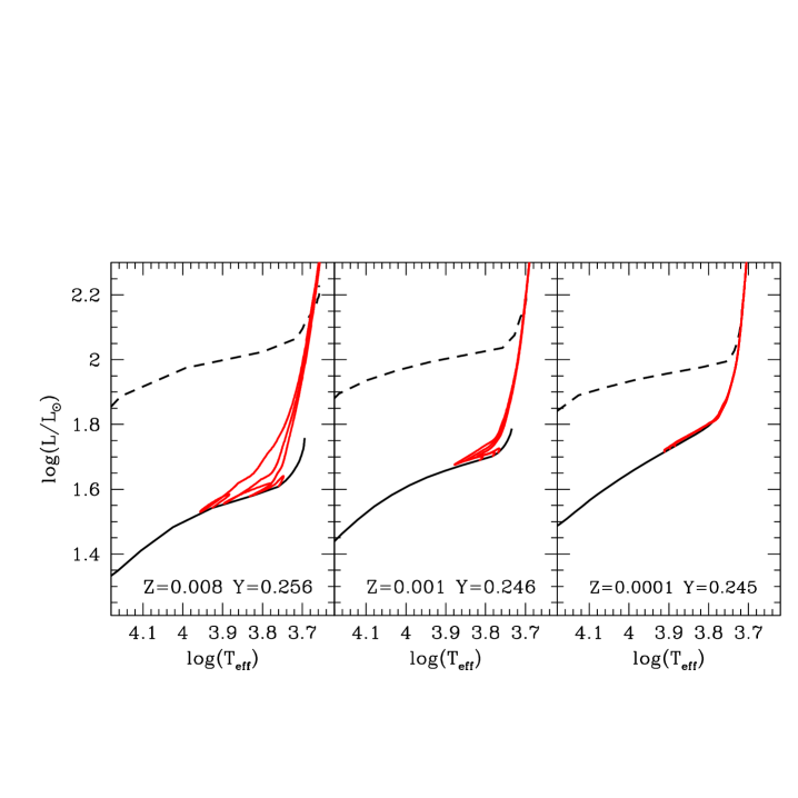
Figure 1.— The Hertzsprung–Russell diagram for three sets of HB evolutionary models. From left to right black solid and dashed lines show the location of the ZAHB and of the central helium exhaustion, respectively. Red lines display HB evolutionary models populating the RRL instability strip. The individual stellar masses are 0.75, 0.76, 0.77 $M/M_{\odot}$ for the most metal-poor (Z=0.0001, right panel), 0.65, 0.66, 0.67 $M/M_{\odot}$ for the metal–intermediate (Z=0.001, middle panel) and 0.56, 0.57, 0.58 $M/M_{\odot}$ for the more metal–rich (Z=0.008, left panel) chemical composition.

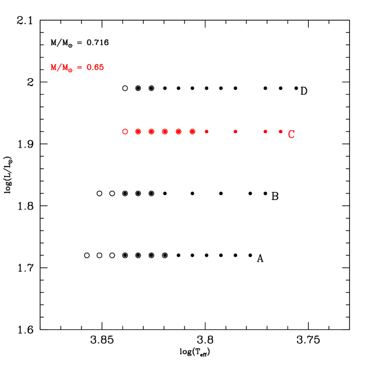
Figure 2.— Location in the Hertzsprung–Russell diagram for a set of RRL models at fixed chemical composition (Z=0.0003, Y=0.245). The FU models are marked with filled circles, while the FOs with open circles. The black symbols mark pulsation models computed assuming the same stellar mass (0.716 M_⊙) and three different luminosity levels: the Zero Age Horizontal Branch (ZAHB, sequence A), a luminosity level 0.1 dex brighter than the ZAHB (sequence B) and the luminosity level of central He exhaustion (sequence D). The red symbols display RRL models computed assuming a stellar mass $\sim$10% smaller (0.65 M_⊙) than the ZAHB mass value and 0.2 dex brighter than the ZAHB luminosity (sequence C). This sequence of pulsation models was computed to account for evolved RRLs. Similar sets of RRL models were computed for the other adopted chemical compositions (see Table LABEL:PARAMETRI).

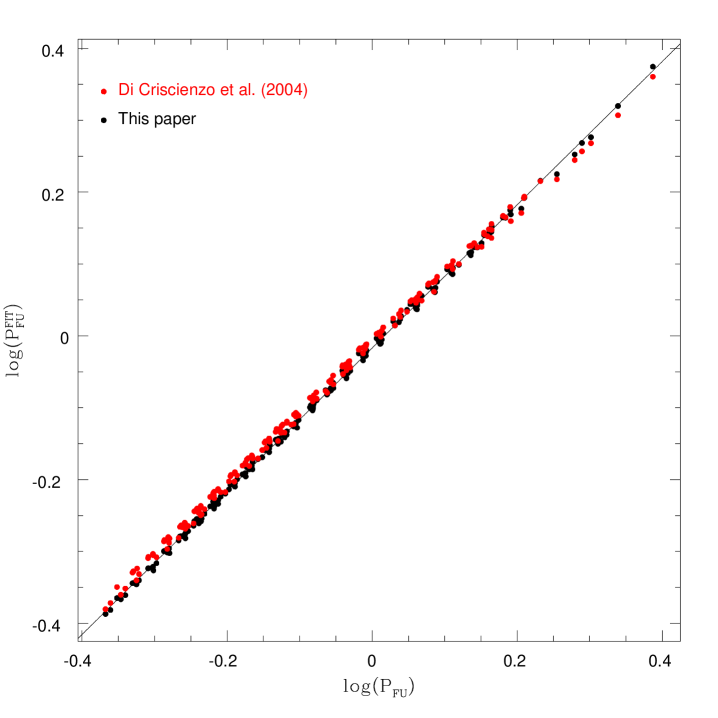
Figure 3.— Comparison between the FU periods ($\log(P_{FU})$) predicted by individual models and the FU periods ($\log(P^{FIT}_{FU})$) given by the pulsation relation provided in this paper (black symbols). The red symbols display the same comparison, but using the pulsation relation provided by Di Criscienzo, Marconi & Caputo (2004).

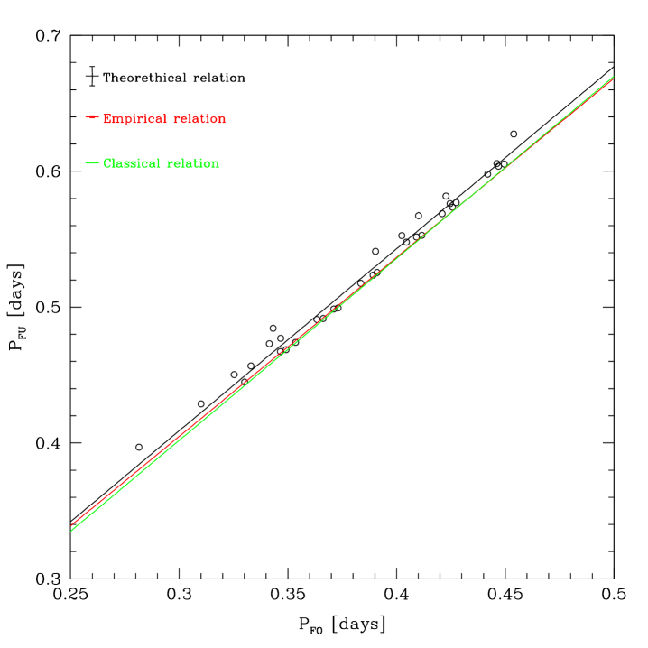
Figure 4.— Relation between FU and FO periods for pulsation models located inside the so-called ”OR region”. The black solid line shows the linear regression based on theoretical models. The red and the green solid lines display the empirical and the classical relation between FU and FO periods (see text for more details).

Figure 5.— Nonlinear total work integral as a function of integration time for three different FO (left panels) and three FU models (right panels). They are centrally located in the middle of the instability strip, and constructed assuming three different metal abundances, stellar masses and luminosity levels (see labeled values).

Figure 6.— bolometric amplitude as a function of the integration time for the same models of Fig.  5.

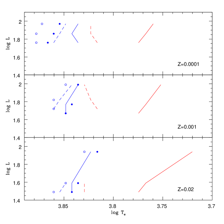
Figure 7.— From top to bottom the panels display predicted instability strips for FU (solid) and FO (dashed) pulsators at three different chemical compositions: $Z=0.0001$ (top panel), $Z=0.001$ (middle) and $Z=0.02$ (bottom). The hot edges are plotted in blue, while the cool edges in red. The linear FOBE and FBE are represented by open and filled blue circles, respectively (see Appendix).

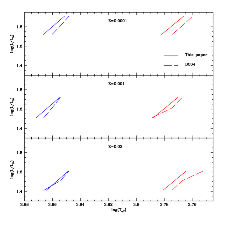
Figure 8.— Comparison between the current instability strip boundaries (solid lines) and similar predictions by Di Criscienzo, Marconi & Caputo (2004) (dashed lines). The blue lines display the FO blue boundaries, while the red lines the FU red boundaries.

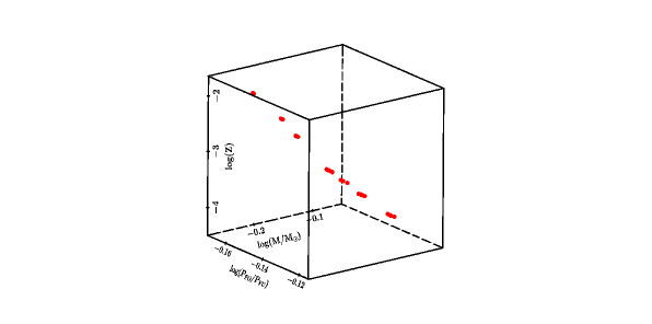
Figure 9.— Tridimensional plot showing the correlation among stellar mass ($\log(M/M_{\odot})$), metallicity ($\log(Z)$) and period ratios ($\log(P_{FO}/P_{FU})$) for the pulsation models located inside the so-called ”OR region”.

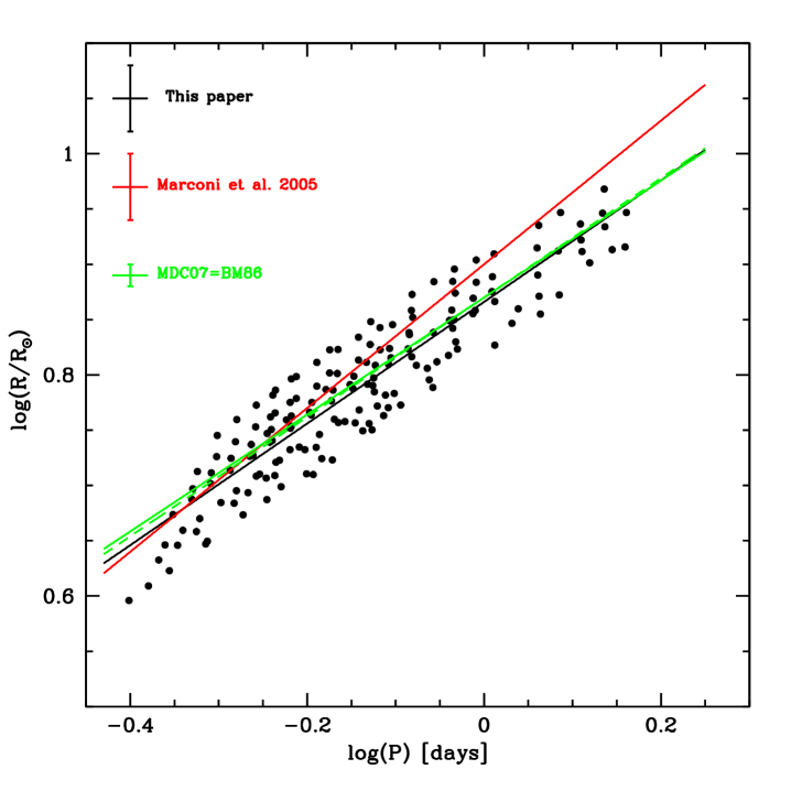
Figure 10.— Period-Radius relation for FU pulsators covering the entire range of chemical compositions adopted in the current investigation. The black solid line depicts the linear regression with a standard deviation of 0.03 dex. The red solid line shows the theoretical PR relation provided by Marconi et al. (2005), while the solid green line the extrapolation to shorter periods of the PR for BL Herculis variables based on pulsation models provided by Marconi & Di Criscienzo (2007). The latter is almost identical to the empirical PR relation provided by Burki & Meylan (1986) for the same class of variable stars and represented in the plot by the dashed green line.

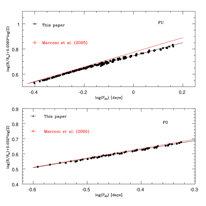
Figure 11.— Period-Radius-Metallicity (PRZ) relations for FU (top panel) and FO (bottom panel) pulsators with a standard deviation of 0.006 and 0.003 dex, respectively. Black lines display the linear regression based on the current models, while the red lines show similar PRZ relations provided by Marconi et al. (2005).

Figure 12.— Predicted bolometric light-curves for FU pulsators at fixed chemical composition ($Z=0.0006$, $Y=0.245$). The models refer to sequence ($M=0.67M_{\odot}$, $\log{L/L_{\odot}}=1.69$). The effective temperatures and the pulsation periods are labeled.

Figure 13.— Same as Figure 12, but for FO pulsators.

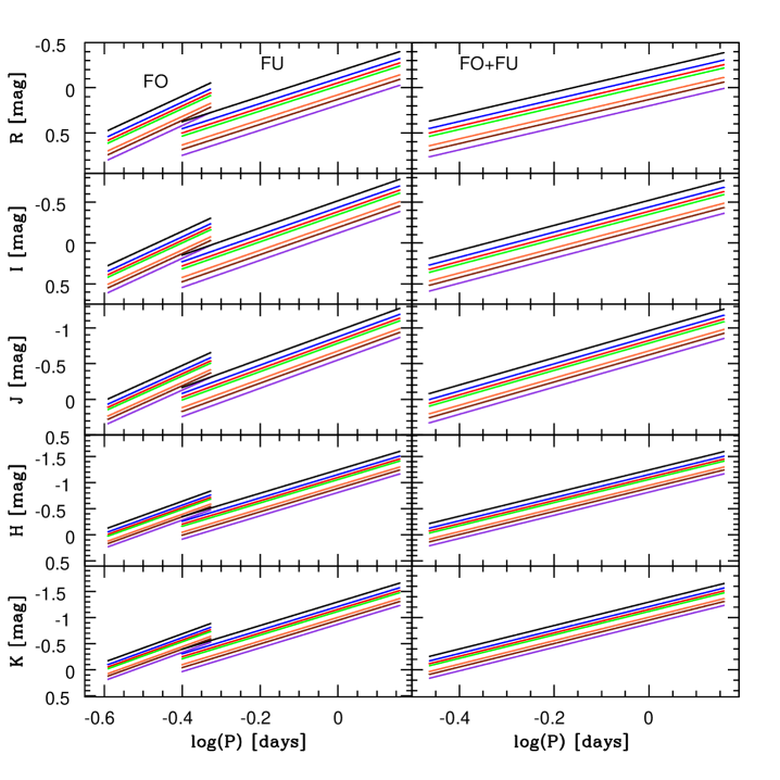
Figure 14.— Left panels – Predicted metal-dependent optical and NIR ($RIJHK$) PL relations FU and FO pulsators. Lines of different colors display predictions with metal abundances ranging from $Z=0.0001$ (black lines) to $Z=0.02$ (purple lines). Right panels – Same as the left ones, but for FU$+$FO pulsators.

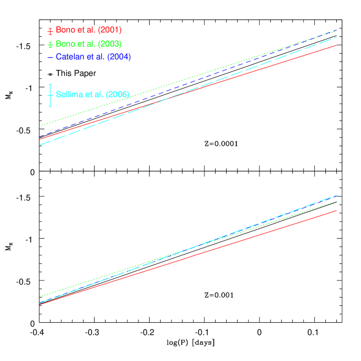
Figure 15.— Comparison among the current PLZ relations for the two different metal abundances (Z=0.0001, top; Z=0.001, bottom) and similar relations available in the literature. The standard deviations of the above PLZ relations, when available, are plotted in the top left corner of the top panel.

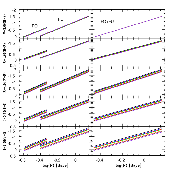
Figure 16.— Left panels – Predicted metal-dependent optical PWZ relations. The color coding is the same as in Figure 14. The coefficients of the color terms are labeled on the Y-axis. Note either the minimal or the marginal metal dependence of the PW(V,B-V) (top panel) and of the PW(R,B-R) (second panel from top). Right panels – Same as the left ones, but for FU$+$FO pulsators.

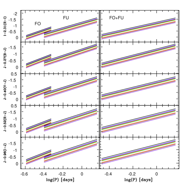
Figure 17.— Same as in Figure 16, but for optical-NIR PWZ relations.

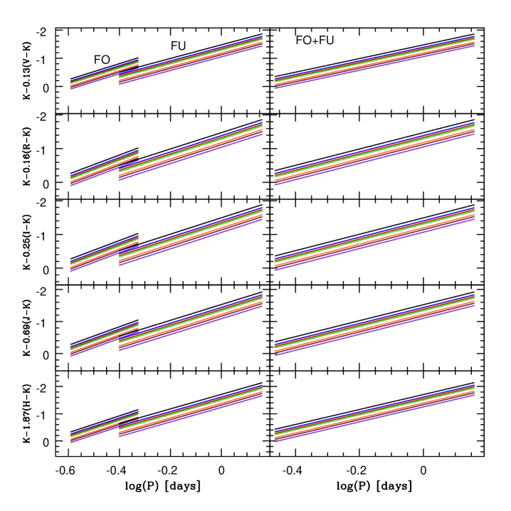
Figure 18.— Same as in Figure 16, but for NIR PWZ relations.

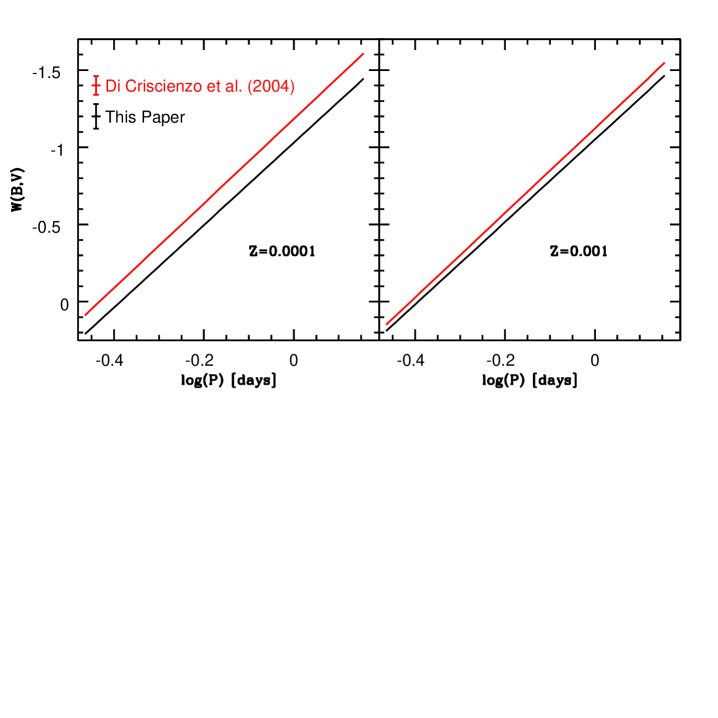
Figure 19.— Comparison between the current PWZ(V,B-V) relations and similar relations provided by Di Criscienzo, Marconi & Caputo (2004) for two different metal abundances: $Z=0.0001$ (top panel) and $Z=0.001$ (bottom panel).

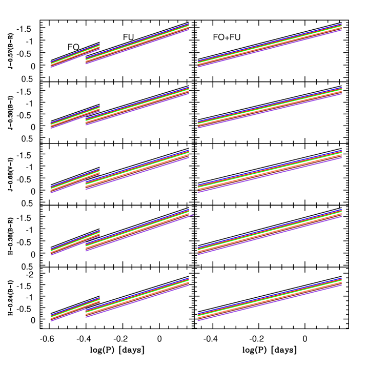
Figure 20.— Left Panels – Predicted metal-dependent triple bands optical-NIR PWZ relations. The color coding is the same as in Figure 16. Right panels – Same as the left ones, but for FU$+$FO pulsators.

Appendix A Linear models

The current set of linear models are purely radiative (Bono & Stellingwerf, 1994) and do not provide an estimate of the red boundaries of the instability strip. The physical mechanism that is providing the quenching of radial oscillation is the increased efficiency of convective transport. However they provide the envelope structures and the linear radial eigenfunctions adopted by the nonlinear hydrodynamical models. The nonlinear analysis is performed by imposing a constant perturbation velocity (5-10 km sec^-1) both to the FU and the FO linear radial eigenfunctions (Bono & Stellingwerf, 1994; Bono, Marconi, & Stellingwerf, 1999). After this initial perturbation the dynamical behavior is followed in time until the radial displacements approach their asymptotic behavior. In the current linear models the inner boundary of the static model is located at a distance of $\approx$10% of the equilibrium photospheric radius. The outer boundary is located at an optical depth $\tau=0.0001$ and the stellar mass attached to the outermost zone is at least one order of magnitude larger than the mass of the surface. The mass zoning of the stellar envelope was fixed assuming a mass ratio between consecutive zones of 1.04 for temperatures cooler than 60,000 K. It was increased by 0.001 in the zones located at higher temperatures. As a whole we ended up with envelope models including typically 200-300 discrete mesh points (Bono et al., 1998), allowing smooth variations of the physical parameters in both driving and damping envelope regions. The envelope mass decreases from 18% to a few percents of the total mass when moving from the blue faint to the red bright pulsation models. The dependence of the envelope mass on chemical composition is negligible.

Fig. 7 shows the comparison between the nonlinear edges of the instability strip (§ 4) and the linear FU (filled circles) and FO (open circles) blue boundaries. We note that the linear FOBE and FBE shows a more evident dependence on the metal content than their nonlinear counterpart when moving from Z=0.0001 to Z=0.02. In particular, for the most metal-poor chemical composition (Z=0.0001, Y=0.245) the linear boundaries are significantly bluer than the nonlinear ones. This is an expected result, because the inclusion of convective transport causes a decrease in pulsation destabilization (driving), therefore, the blue edges move towards lower effective temperatures. The quenching caused by convection, close to the blue edges of the instability strip, becomes less efficient in the metal-rich regime. It is partially counterbalanced by the driving of the K-bump, i.e. the radiative opacity peak located at $\approx$250,000 K (Seaton et al., 1994; Rogers & Iglesias, 1992; Bono et al., 1996).

References

- Abbas et al. (2014) Abbas, M. A., Grebel, E. K., Martin, N. F., et al. 2014, MNRAS, 441, 1230
- Alcock et al. (1999) Alcock, C., Allsman, R. A., Alves, D., et al. 1999, ApJ, 511, 185
- Ade et al. (2014) Ade, P. A. R., Aikin, R. W., Amiri, M., et al. 2014, ApJ, 792, 62
- Ade et al. (2014) Planck Collaboration, Ade, P. A. R., Aghanim, N., et al. 2014, A&A, 571, A16
- Alexander & Ferguson (1994) Alexander, D. R., Ferguson, J. W. 1994, ApJ, 437, 879
- Beaulieu et al. (1997) Beaulieu, J. P., Krockenberger, M., Sasselov, D. D., et al. 1997, A&A, 321, L5
- Benkő et al. (2011) Benkő, J. M., Szabó, R., & Paparó, M. 2011, MNRAS, 417, 974
- Bessell (1990) Bessell, M. S. 1990, PASP, 102, 1181
- Bono & Stellingwerf (1993) Bono, G., & Stellingwerf, R. F. 1993, IAU Colloq. 139: New Perspectives on Stellar Pulsation and Pulsating Variable Stars, 275
- Bono & Stellingwerf (1994) Bono, G., Stellingwerf, R.F. 1994, ApJS, 93, 233
- Bono et al. (1995) Bono, G., Caputo, F., Castellani, V., Marconi, M. 1995, ApJ, 448, 115
- Bono et al. (1995) Bono, G., Caputo, F., & Marconi, M. 1995, AJ, 110, 2365
- Bono et al. (1995) Bono, G., Caputo, F., Castellani, V., et al. 1995c, ApJ, 442, 159
- Bono et al. (1995) Bono, G., Caputo, F., & Stellingwerf, R. F. 1995, ApJS, 99, 263
- Bono et al. (1996) Bono, G., Caputo, F., Castellani, V., & Marconi, M. 1996, ApJ, 471, L33
- Bono et al. (1996) Bono, G., Incerpi, R., & Marconi, M. 1996, ApJ, 467, L97
- Bono et al. (1997) Bono, G., Caputo, F., Cassisi, S., Castellani, V., & Marconi, M. 1997, ApJ, 479, 279
- Bono et al. (1997) Bono, G., Caputo, F., Cassisi, S., Incerpi, R., & Marconi, M. 1997, ApJ, 483, 811
- Bono et al. (1997) Bono, G., Caputo, F., Castellani, V., & Marconi, M. 1997, A&AS, 121, 327
- Bono et al. (1998) Bono, G., Caputo, F., & Marconi, M. 1998, ApJ, 497, L43
- Bono, Marconi, & Stellingwerf (1999) Bono, G., Marconi, M., Stellingwerf, R.F. 1999, ApJS, 122, 167
- Bono et al. (2000) Bono, G., Castellani, V., & Marconi, M. 2000, ApJ, 532, L129
- Bono et al. (2001) Bono, G., Caputo, F., Castellani, V., Marconi, M., & Storm, J. 2001, MNRAS, 326, 1183
- Bono et al. (2002) Bono, G., Caputo, F., Castellani, V., Marconi, M., & Storm, J. 2002, MNRAS, 332, L78
- Bono et al. (2002) Bono, G., Caputo, F., Marconi, M., & Santolamazza, P. 2002, Observational Aspects of Pulsating B- and A Stars, 256, 249
- Bono et al. (2002c) Bono, G., Castellani, V., & Marconi, M. 2002, ApJ, 565, L83
- Bono et al. (2003) Bono, G., Caputo, F., Castellani, V., Marconi, M., Storm, J., Degl’Innocenti, S. 2003, MNRAS, 344, 1097
- Bono et al. (2010) Bono, G., Caputo, F., Marconi, M., & Musella, I. 2010, ApJ, 715, 277
- Bono et al. (2011) Bono, G., Dall’Ora, M., Caputo, F., et al. 2011, RR Lyrae Stars, Metal-Poor Stars, and the Galaxy, 1
- Bono, Salaris & Gilmozzi (2013) Bono, G., Salaris, M. & Gilmozzi, R. 2013, A&A, 549, 102
- Braga et al. (2014) Braga, V. F., Dall’Ora, M., Bono, G., et al. 2014, arXiv:1411.6826
- Bragaglia et al. (2001) Bragaglia, A., Gratton, R. G., Carretta, E., et al. 2001, AJ, 122, 207
- Buchler & Goupil (1984) Buchler, J. R., & Goupil, M.-J. 1984, ApJ, 279, 394
- Buchler et al. (1999) Buchler, J. R., Yecko, P., Kolláth, Z., & Goupil, M.-J. 1999, Stellar Structure: Theory and Test of Connective Energy Transport, 173, 141
- Burki & Meylan (1986) Burki, G., & Meylan, G. 1986, A&A, 159, 255
- Cacciari et al. (2000) Cacciari, C., Clementini, G., Castelli, F., & Melandri, F. 2000, IAU Colloq. 176: The Impact of Large-Scale Surveys on Pulsating Star Research, 203, 176
- Cacciari & Clementini (2003) Cacciari, C., & Clementini, G. 2003, Stellar Candles for the Extragalactic Distance Scale, 635, 105
- Caputo et al. (2000) Caputo, F., Castellani, V., Marconi, M., Ripepi, V. 2000, MNRAS, 316, 819
- Caputo et al. (2000) Caputo, F., Marconi, M., Musella, I., & Santolamazza, P. 2000, A&A, 359, 1059
- Caputo et al. (2004) Caputo, F., Castellani, V., Degl’Innocenti, S., Fiorentino, G., & Marconi, M. 2004, A&A, 424, 927
- Cardelli et al. (1989) Cardelli, J. A., Clayton, G. C., & Mathis, J. S. 1989, ApJ, 345, 245
- Cassisi et al. (1998) Cassisi, S., Castellani, V., degl’Innocenti, S., & Weiss, A. 1998, A&AS, 129, 267
- Cassisi et al. (2003) Cassisi, S., Salaris, M., & Irwin, A. W. 2003, ApJ, 588, 862
- Cassisi et al. (2004) Cassisi, S., Castellani, M., Caputo, F., & Castellani, V. 2004, A&A, 426, 641
- Cassisi et al. (2007) Cassisi, S., Potekhin, A. Y., Pietrinferni, A., Catelan, M., & Salaris, M. 2007, ApJ, 661, 1094
- Cassisi et al. (2008) Cassisi, S., Salaris, M., Pietrinferni, A. et al. 2008, ApJ, 672,L115
- Castellani et al. (1991) Castellani, V., Chieffi, A., & Pulone, L. 1991, ApJS, 76, 911
- Castellani (1983) Castellani, V. 1983, Mem. Soc. Astron. Italiana, 54, 141
- Castelli, Gratton & Kurucz (1997a) Castelli, F., Gratton, R. G., & Kurucz, R. L. 1997a, A&A, 318, 841
- Castelli, Gratton & Kurucz (1997b) Castelli, F., Gratton, R. G., & Kurucz, R. L. 1997b, A&A, 324, 432
- Castor (1971) Castor, J. I. 1971, ApJ, 166, 109
- Catelan et al. (2004) Catelan, M., Pritzl, B. J., & Smith, H. A. 2004, ApJS, 154, 633
- Christy (1967) Christy, R. F. 1967, PASP, 79, 429
- Coppola et al. (2011) Coppola, G., Dall’Ora, M., Ripepi, V., et al. 2011, MNRAS, 416, 1056
- Coppola et al. (2013) Coppola, G., Stetson, P. B., Marconi, M., et al. 2013, ApJ, 775, 6
- Cox (1963) Cox, J. P. 1963, ApJ, 138, 487
- Cox (1974) Cox, A. N. 1974, Stellar Instability and Evolution, 59, 39
- Cusano et al. (2013) Cusano, F., Clementini, G., Garofalo, A., et al. 2013, ApJ, 779, 7
- Cutri et al. (2003) Cutri, R. M., Skrutskie, M. F., van Dyk, S., et al. 2003, ”The IRSA 2MASS All-Sky Point Source Catalog, NASA/IPAC Infrared Science Archive. ¡A href=”http://irsa.ipac.caltech.edu/applications/Gator/”¿http://irsa.ipac.caltech.edu/applications/Gator/¡/A¿”,
- Dall’Ora et al. (2004) Dall’Ora, M., Storm, J., Bono, G., et al. 2004, ApJ, 610, 269
- Dambis et al. (2014) Dambis, A. K., Rastorguev, A. S., & Zabolotskikh, M. V. 2014, MNRAS, 439, 3765
- Di Criscienzo, Marconi & Caputo (2004) Di Criscienzo, M., Marconi, M., Caputo, F. 2004, ApJ, 612, 1092
- Di Criscienzo et al. (2011) Di Criscienzo, M., Greco, C., Ripepi, V., et al. 2011, AJ, 141, 81
- Dorfi & Feuchtinger (1999) Dorfi, E. A., & Feuchtinger, M. U. 1999, A&A, 348, 815
- Drake et al. (2013) Drake, A. J., Catelan, M., Djorgovski, S. G., et al. 2013, ApJ, 763, 32
- Ertel et al. (2014) Ertel, S., Absil, O., Defrère, D., et al. 2014, A&A, 570, AA128
- Feuchtinger (1999) Feuchtinger, M. U. 1999, A&A, 351, 103
- Fiorentino et al. (2002) Fiorentino, G., Caputo, F., Marconi, M., & Musella, I. 2002, ApJ, 576, 402
- Fiorentino et al. (2007) Fiorentino, G., Marconi, M., Musella, I., & Caputo, F. 2007, A&A, 476, 863
- Fiorentino et al. (2010) Fiorentino, G., Monachesi, A., Trager, S. C., et al. 2010, ApJ, 708, 817
- Fiorentino et al. (2012) Fiorentino, G., Contreras Ramos, R., Tolstoy, E., Clementini, G., & Saha, A. 2012, A&A, 539, AA138
- Fiorentino et al. (2013) Fiorentino, G., Musella, I., & Marconi, M. 2013, MNRAS, 434, 2866
- Fiorentino et al. (2014) Fiorentino, G., Bono, G., Monelli, M., et al. 2014, arXiv:1411.7300
- Fitzpatrick & Massa (2009) Fitzpatrick, E. L., & Massa, D. 2009, ApJ, 699, 1209
- Gallenne et al. (2014) Gallenne, A., Mérand, A., Kervella, P., et al. 2014, A&A, 561, LL3
- Gezari et al. (2013) Gezari, S., Martin, D. C., Forster, K., et al. 2013, ApJ, 766, 60
- Grevesse et al. (1993) Grevesse, N., Noels, A., & Sauval, A. J. 1993, A&A, 271, 587
- Groenewegen et al. (2008) Groenewegen, M. A. T., Udalski, A., & Bono, G. 2008, A&A, 481, 441
- Hinshaw et al. (2013) Hinshaw, G., Larson, D., Komatsu, E., et al. 2013, ApJS, 208, 19
- Iben & Rood (1970) Iben, I., Jr., & Rood, R. T. 1970, ApJ, 161, 587
- Iglesias & Rogers (1996) Iglesias, C., Rogers, F. J. 1996, ApJ, 464, 943
- Inno et al. (2013) Inno, L., Matsunaga, N., Bono, G., et al. 2013, ApJ, 764, 84
- Kervella (2008) Kervella, P. 2008, 14th Cambridge Workshop on Cool Stars, Stellar Systems, and the Sun, 384, 189
- Kervella et al. (2001) Kervella, P., Coudé du Foresto, V., Perrin, G., et al. 2001, A&A, 367, 876
- Kinemuchi et al. (2006) Kinemuchi, K., Smith, H. A., Woźniak, P. R., McKay, T. A., & ROTSE Collaboration 2006, AJ, 132, 1202
- Kinman & Brown (2014) Kinman, T. D., & Brown, W. R. 2014, AJ, 148, 121
- Kolláth et al. (1998) Kolláth, Z., Beaulieu, J. P., Buchler, J. R., & Yecko, P. 1998, ApJ, 502, L55
- Kovács (2000) Kovács, G. 2000, A&A, 363, L1
- Kovács & Walker (1999) Kovács, G., & Walker, A. R. 1999, ApJ, 512, 271
- Kučinskas et al. (2006) Kučinskas, A., Hauschildt, P. H., Brott, I., et al. 2006, A&A, 452, 1021
- Kuehn et al. (2013) Kuehn, C. A, Smith, H. A., Catelan, M., et al. 2013, arXiv:1310.0553
- Kunder et al. (2013) Kunder, A., Stetson, P. B., Cassisi, S., et al. 2013, AJ, 146, 119
- Landolt (1992) Landolt, A. U. 1992, AJ, 104, 372
- Longmore et al. (1986) Longmore, A. J., Fernley, J. A., & Jameson, R. F. 1986, MNRAS, 220, 279
- Longmore et al. (1990) Longmore, A. J., Dixon, R., Skillen, I., Jameson, R. F., & Fernley, J. A. 1990, MNRAS, 247, 684
- Madore (1982) Madore, B. F. 1982, ApJ, 253, 575
- Madore & Freedman (2012) Madore, B. F., & Freedman, W. L. 2012, ApJ, 744, 132
- Marconi et al. (2003) Marconi, M., Caputo, F., Di Criscienzo, M., Castellani, M. 2003, ApJ, 596, 299
- Marconi et al. (2005) Marconi, M., Nordgren, T., Bono, G., Schnider, G., & Caputo, F. 2005, ApJ, 623, L133
- Marconi & Clementini (2005) Marconi, M., & Clementini, G. 2005, AJ, 129, 2257
- Marconi & Degl’Innocenti (2007) Marconi, M., & Degl’Innocenti, S. 2007, A&A, 474, 557
- Marconi & Di Criscienzo (2007) Marconi, M., & Di Criscienzo, M. 2007, A&A, 467, 223
- Marconi (2009) Marconi, M. 2009, American Institute of Physics Conference Series, 1170, 223
- Marconi et al. (2011) Marconi, M., Bono, G., Caputo, F., et al. 2011, ApJ, 738, 111
- Marconi (2012) Marconi, M. 2012, Memorie della Societa Astronomica Italiana Supplementi, 19, 138
- Marconi et al. (2013) Marconi, M., Molinaro, R., Bono, G., et al. 2013, ApJ, 768, LL6
- Matsunaga et al. (2009) Matsunaga, N., Feast, M. W., & Menzies, J. W. 2009, MNRAS, 397, 933
- Matsunaga et al. (2013) Matsunaga, N., Feast, M. W., Kawadu, T., et al. 2013, MNRAS, 429, 385
- McCall (2004) McCall, M. L. 2004, AJ, 128, 2144
- Miceli et al. (2008) Miceli, A., Rest, A., Stubbs, C. W., et al. 2008, ApJ, 678, 865
- Minniti et al. (2014) Minniti, D., Saito, R. K., Gonzalez, O. A., et al. 2014, A&A, 571, AA91
- Moretti et al. (2009) Moretti, M. I., Dall’Ora, M., Ripepi, V., et al. 2009, ApJ, 699, L125
- Moretti et al. (2014) Moretti, M. I., Clementini, G., Muraveva, T., et al. 2014, MNRAS, 437, 2702
- Musella et al. (2012) Musella, I., Ripepi, V., Marconi, M., et al. 2012, ApJ, 756, 121
- Natale et al. (2008) Natale, G., Marconi, M., & Bono, G. 2008, ApJ, 674, L93
- Ngeow & Kanbur (2005) Ngeow, C.-C., & Kanbur, S. M. 2005, MNRAS, 360, 1033
- Nordgren et al. (2000) Nordgren, T. E., Armstrong, J. T., Germain, M. E., et al. 2000, ApJ, 543, 972
- Pedicelli et al. (2009) Pedicelli, S., Bono, G., Lemasle, B., et al. 2009, A&A, 504, 81
- Petersen (1991) Petersen, J. O. 1991, A&A, 243, 426
- Piersimoni et al. (2002) Piersimoni, A. M., Bono, G., & Ripepi, V. 2002, AJ, 124, 1528
- Pietrinferni et al. (2004) Pietrinferni, A., Cassisi, S., Salaris, M., & Castelli, F. 2004, ApJ, 612, 168
- Pietrinferni et al. (2006) Pietrinferni, A., Cassisi, S., Salaris, M., Castelli, F. 2006, ApJ, 642, 797
- Pietrinferni et al. (2013) Pietrinferni, A., Cassisi, S., Salaris, M., & Hidalgo, S. 2013, A&A, 558, A46
- Pietrukowicz et al. (2014) Pietrukowicz, P., Kozlowski, S., Skowron, J., et al. 2014, arXiv:1412.4121
- Ade et al. (2014) Planck Collaboration, Ade, P. A. R., Aghanim, N., et al. 2014, A&A, 571, A16
- Pojmański (2014) Pojmański, G. 2014, Contributions of the Astronomical Observatory Skalnate Pleso, 43, 523
- Popielski et al. (2000) Popielski,B. L., Dziembowski, W. A., & Cassisi, S. 2000, Acta Astronomica, 50, 491
- Pryke et al. (2002) Pryke, C., Halverson, N. W., Leitch, E. M., et al. 2002, ApJ, 568, 46
- Renzini (1983) Renzini, A. 1983, Mem. Soc. Astron. Italiana, 54, 335
- Riess et al. (2011) Riess, A. G., Macri, L., Casertano, S., et al. 2011, ApJ, 730, 119
- Riess et al. (2012) Riess, A. G., Macri, L., Casertano, S., et al. 2012, ApJ, 752, 76
- Ripepi et al. (2007) Ripepi, V., Clementini, G., Di Criscienzo, M., et al. 2007, ApJ, 667, L61
- Ripepi et al. (2012) Ripepi, V., Moretti, M. I., Marconi, M., et al. 2012, MNRAS, 424, 1807
- Ripepi et al. (2015) Ripepi, V., Moretti, M. I., Marconi, M., et al. 2015, MNRAS, 446, 3034
- Rogers & Iglesias (1992) Rogers, F. J., & Iglesias, C. A. 1992, ApJS, 79, 507
- Romaniello et al. (2008) Romaniello, M., Primas, F., Mottini, M., et al. 2008, A&A, 488, 731
- Ryan et al. (1991) Ryan, S. G., Norris, J. E., & Bessell, M. S. 1991, AJ, 102, 303
- Salaris (2013) Salaris, M. 2013, IAU Symposium, 289, 145
- Sandage (1990) Sandage, A. 1990, ApJ, 350, 603
- Sandage (1993) Sandage, A. 1993, AJ, 106, 703
- Seaton et al. (1994) Seaton, M. J., Yan, Y., Mihalas, D., & Pradhan, A. K. 1994, MNRAS, 266, 805
- Serenelli & Basu (2010) Serenelli, A. M., & Basu, S. 2010, ApJ, 719, 865
- Sesar et al. (2011) Sesar, B., Stuart, J. S., Ivezić, Ž., et al. 2011, AJ, 142, 190
- Sesar et al. (2013) Sesar, B., Ivezić, Ž., Stuart, J. S., et al. 2013, AJ, 146, 21
- Sesar et al. (2014) Sesar, B., Banholzer, S. R., Cohen, J. G., et al. 2014, ApJ, 793, 135
- Smolec & Moskalik (2008a) Smolec, R., & Moskalik, P. 2008, Acta Astronomica, 58, 193
- Smolec & Moskalik (2008b) Smolec, R., & Moskalik, P. 2008, iActa Astronomica, 58, 233
- Smolec & Moskalik (2010) Smolec, R., Moskalik, P. 2010, A&A, 524, 40
- Smolec et al. (2013) Smolec, R., Pietrzyński, G., Graczyk, D., et al. 2013, MNRAS, 428, 3034
- Sollima et al. (2006) Sollima, A. et al. 2006, ApJ, 640, 43
- Soszyński et al. (2009) Soszyński, I., Udalski, A., Szymański, M. K., et al. 2009, Acta Astronomica, 59, 1
- Soszyński et al. (2010) Soszyński, I., Udalski, A., Szymański, M. K., et al. 2010, Acta Astronomica, 60, 165
- Soszyński et al. (2011) Soszyński, I., Dziembowski, W. A., Udalski, A., et al. 2011, Acta Astronomica, 61, 1
- Soszyński et al. (2014) Soszyński, I., Udalski, A., Szymański, M. K., et al. 2014, Acta Astronomica, 64, 177
- Stellingwerf (1974) Stellingwerf, R. F. 1974, ApJ, 192, 139
- Stellingwerf (1975) Stellingwerf, R. F. 1975, ApJ, 195, 441
- Stellingwerf (1982) Stellingwerf, R. F. 1982, ApJ, 262, 330
- Stellingwerf (1983) Stellingwerf, R. F. 1983, ApJ, 271, 876
- Stetson et al. (2014) Stetson, P. B., Fiorentino, G., Bono, G., et al. 2014, PASP, 126, 616
- Storm et al. (1994) Storm, J., Carney, B. W., & Latham, D. W. 1994, A&A, 290, 443
- Storm et al. (2011) Storm, J., Gieren, W., Fouqué, P., et al. 2011, A&A, 534, AA95
- Szabó et al. (2004) Szabó, R., Kolláth, Z., & Buchler, J. R. 2004, A&A, 425, 627
- Torrealba et al. (2014) Torrealba, G., Catelan, M., Drake, A. J., et al. 2014, VizieR Online Data Catalog, 744, 62251
- Valle et al. (2013) Valle, G., Dell’Omodarme, M., Prada Moroni, P. G., & Degl’Innocenti, S. 2013, A&A, 549, AA50
- van Albada & Baker (1971) van Albada, T. S., & Baker, N. 1971, ApJ, 169, 311
- van Albada & Baker (1973) van Albada, T. S., & Baker, N. 1973, ApJ, 185, 477
- van den Bergh (1975) van den Bergh, S. 1975, Galaxies and the Universe, 509
- VandenBerg (2013) VandenBerg, D. A. 2013, IAU Symposium, 289, 161
- Vivas & Zinn (2006) Vivas, A. K., & Zinn, R. 2006, AJ, 132, 714
- Walker & Terndrup (1991) Walker, A. R., & Terndrup, D. M. 1991, ApJ, 378, 119
- Zinn et al. (2014) Zinn, R., Horowitz, B., Vivas, A. K., et al. 2014, ApJ, 781, 22