Dense Clumps and Candidates for Molecular Outflows in W40

Abstract

We report results of the ${\rm{}^{12}CO}$ ($J=3-2$) and ${\rm HCO^{+}}$ ($J=4-3$) observations of the W40 H ii region with the ASTE 10 m telescope (HPBW$\simeq 22\arcsec$) to search for molecular outflows and dense clumps. We found that the velocity field in the region is highly complex, consisting of at least four distinct velocity components at $V_{\rm LSR}\simeq 3$, 5, 7, and 10 km s${}^{-1}\,$. The $\sim$7 km s${}^{-1}\,$component represents the systemic velocity of cold gas surrounding the entire region, and causes heavy absorption in the ${\rm{}^{12}CO}$ spectra over the velocity range $6\lesssim V_{\rm LSR}\lesssim 9$ km s${}^{-1}\,$. The $\sim$5 and $\sim$10 km s${}^{-1}\,$components exhibit high ${\rm{}^{12}CO}$ temperature ($\gtrsim 40$ K) and are found mostly around the H ii region, suggesting that these components are likely to be tracing dense gas interacting with the expanding shell around the H ii region. Based on the ${\rm{}^{12}CO}$ data, we identified 13 regions of high velocity gas which we interpret as candidate outflow lobes. Using the ${\rm HCO^{+}}$ data, we also identified six clumps and estimated their physical parameters. On the basis of the ASTE data and near-infrared images from 2MASS, we present an updated three-dimensional model of this region. In order to investigate molecular outflows in W40, the SiO ($J=1-0$, $v=0$) emission line and some other emission lines at 40 GHz were also observed with the 45 m telescope at the Nobeyama Radio Observatory, but they were not detected at the present sensitivity.

1 INTRODUCTION

The W40 complex is a site of active star formation in the Aquila Rift containing molecular clouds, star cluster, massive stars, and an H ii region. Several mid and far-infrared observations have revealed that the W40 complex consists of a number of filamentary structures to form an hourglass shape (e.g., Rodney & Reipurth, 2008; Kuhn et al., 2010; André et al., 2010; Bontemps et al., 2010; Könyves et al., 2010). There are a number of young stellar objects (YSOs) associated with this complex (e.g., Rodríguez et al., 2010; Kuhn et al., 2010; Maury et al., 2011; Mallick et al., 2013). The cluster and its associated H ii region are located to the northwest of the constriction of the hourglass. The cluster is found to have a considerably large stellar surface density of $\sim 650$ pc^-2 (Mallick et al., 2013). Several ionizing sources for the H ii region are also found in this region. IRS 1A South is an O9.5 spectral type star (Shuping et al., 2012) and is the most luminous source. Another high mass star, IRS 5, is located in the northwest of IRS 1A South. This is classified as a B1V type star (Shuping et al., 2012; Mallick et al., 2013). Radio emission from a roughly spherical compact H ii region has been detected around IRS 5 by Mallick et al. (2013). They suggested that high-mass star formation is going on therein.

Previous molecular line and radio continuum observations revealed the presence of the dense gas around the W40 H ii region (e.g., Zeilik & Lada, 1978; Zhu et al., 2006; Pirogov et al., 2013; Maury et al., 2011). Dobashi et al. (2005) and Dobashi (2011) named the dense region as TGU 279-P7 and No.1195, based on the Digitized Sky Survey (DSS) and the Two Micron All Sky Survey (2MASS) extinction data, respectively. The dense region has a ring-like shape along the boundary of the H ii region (Maury et al., 2011). Pirogov et al. (2013) carried out multiple-molecular line observations such as HCO⁺, CS, and NH₃, and found the large variations of the fractional abundances of these molecules over the dense region. All of these studies indicate that the H ii region is strongly interacting with the surrounding dense gas. The W40 complex is therefore an excellent region to study the interaction of massive stars with their parental molecular cloud.

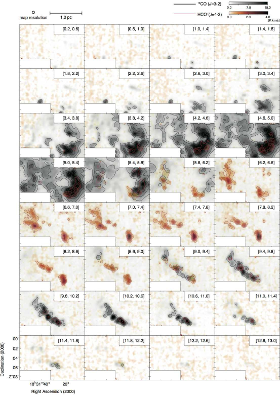
Figure 2: Channel maps of the ${\rm{}^{12}CO}$ ($J=3-2$) (gray) and ${\rm HCO^{+}}$ ($J=4-3$) (red) emission lines in the velocity range $0.2\leqq V_{\rm LSR}\leqq 13.0$ km s${}^{-1}\,$with the 0.4 km s${}^{-1}\,$step. The velocity range in units of km s${}^{-1}\,$used for the integration is indicated at the top right corner of each panel. The lowest contours and the contour intervals are 3 K km s${}^{-1}\,$for the ${\rm{}^{12}CO}$ maps, and are 0.3 K km s${}^{-1}\,$for the ${\rm HCO^{+}}$ maps.

Several studies have discussed the geometry of the W40 complex (e.g., Crutcher, 1977; Vallee, 1987; Kuhn et al., 2010; Pirogov et al., 2013). Especially, Vallee (1987) suggested the blister model for W40 which is illustrated in their Figure 2 and is now regarded as a standard picture of the region. However, the complex velocity structure has prevented us from complete understanding of the geometry and kinematics of the molecular cloud associated with W40 (e.g., Crutcher, 1977; Pirogov et al., 2013). More detailed studies to uncover the internal density distribution and kinematics of the molecular cloud is needed to better understand the structure of this region.

Low-mass members of this region were also revealed by Maury et al. (2011) and Mallick et al. (2013). They identified a number of Class 0/I sources and starless cores around the H ii region. However, outflow activity in this region remains uncertain. Zhu et al. (2006) discovered a weak molecular outflow through their ${\rm{}^{12}CO}$ ($J=3-2$) observations with the KOSMA 3 m telescope whose half power beam width (HPBW) is $\sim 80\arcsec$. The identified outflow lobes appear to have complicated structure. In addition, the surveyed area is limited to a small region just around the H ii region. It is important to carry out a comprehensive survey for molecular outflows covering much wider area to reveal the star formation activity in this region.

In this paper, we present results of the ${\rm{}^{12}CO}$ ($J=3-2$) and ${\rm HCO^{+}}$ ($J=4-3$) observations made toward a large area ($\sim 8\arcmin\times 8\arcmin$) covering the whole W40 H ii region and its interacting molecular cloud, using Atacama Submillimeter Telescope Experiment (ASTE) 10 m telescope. For the purpose of an outflow survey, we carried out ${\rm{}^{12}CO}$ ($J=3-2$) mapping observations to detect 13 outflow candidates. In order to explore the velocity and spatial distributions of the dense gas in the W40 region, we also carried out ${\rm HCO^{+}}$ ($J=4-3$) observations to identify six clumps, and further attempted to model their locations relative to the H ii region along the line-of-sight mainly through a comparison with the 2MASS near-infrared images.

Hereafter we will refer to the observed region simply as W40. The distance estimation to W40 remains uncertain, and varies from 340 to 600 pc depending on the methods used (e.g., Rodney & Reipurth, 2008; Kuhn et al., 2010; Shuping et al., 2012). Here, we adopt the latest estimate of 500 pc derived by Shuping et al. (2012) throughout this paper.

2 OBSERVATIONS

2.1 ¹²CO and HCO⁺ Observations with the ASTE 10 m Telescope

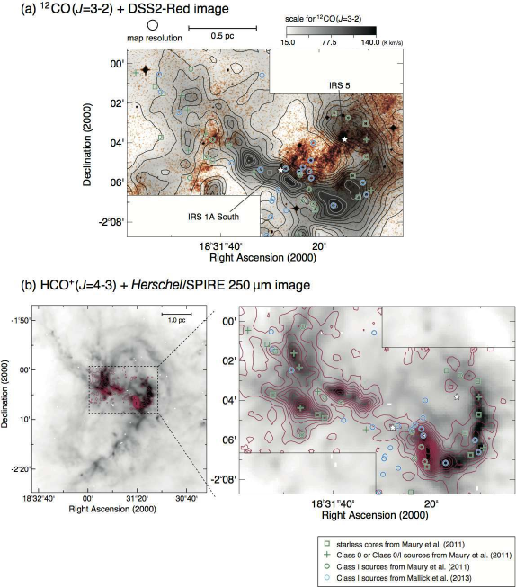
Figure 1: Integrated intensity maps of the (a) ${\rm{}^{12}CO}$ ($J=3-2$) emission line and (b) ${\rm HCO^{+}}$ ($J=4-3$) emission line around W40 obtained with the ASTE telescope. Velocity ranges used for the integration are $-3.0\leqq V_{\rm LSR}\leqq 15.0$ km s${}^{-1}\,$and $3.0\leqq V_{\rm LSR}\leqq 11.4$ km s${}^{-1}\,$for the ${\rm{}^{12}CO}$ and ${\rm HCO^{+}}$ maps, respectively. The lowest contours and the contour intervals for the map in panel (a) are 10 K km s${}^{-1}\,$, and those in panel (b) are 1 K km s${}^{-1}\,$. The red color scale in panel (a) is the DSS2-Red image, and the gray scale in panel (b) is the Herschel SPIRE 250 $\micron$ image. Positions of the high mass IRS sources (IRS 1A Sourth and IRS 5, Shuping et al., 2012) are indicated by star marks. Squares, plus signs, and circles denote the starless cores and Class 0/I sources classified by Maury et al. (2011) (colored in green) and Mallick et al. (2013) (colored in blue). The map resolution ($31\arcsec$) and a linear scale of 0.5 pc (at $D$=500 pc) are shown at the top of panel (a). The area enclosed by the thin lines in panel (a) and right side of panel (b) denotes the observed region.

The mapping observations of W40 were performed with the ${\rm{}^{12}CO}$ ($J=3-2$) and ${\rm HCO^{+}}$ ($J=4-3$) emission lines at 345.795991 GHz and 356.734242 GHz, respectively, using the ASTE 10 m telescope (Ezawa et al., 2004; Kohno et al., 2004) at Atacama, Chile. Data of these molecular lines were obtained simultaneously during the period between 2013 September 26th and October 1st. The area observed is denoted in Figure 1, which covers the central part of the W40 H ii region. The angular resolution of the telescope is HPBW$\simeq 22\arcsec$ at the observed frequencies. A side-band separating (2SB) mixer receiver CATS345 was used for the observations. The spectrometer was an XF-type digital spectro-correlator, called MAC, with 1024 channels covering a bandwidth of 128 MHz. The frequency resolution was 125 kHz, corresponding to a velocity resolution of 0.1 km s${}^{-1}\,$at the observed frequencies. The system noise temperature $T_{\rm sys}$ was $300-400$ K during the observations. The observations were made using the on-the-fly (OTF) mapping technique (Sawada et al., 2008). Data were calibrated with the standard chopper-wheel method (Kutner & Ulich, 1981). The telescope pointing was regularly checked every 1.5 hour using ${\rm{}^{12}CO}$ ($J=3-2$) line from W-Aql, and the pointing error was smaller than $2\arcsec$ during the observations. In addition, we checked the intensity reproducibility by observing M17SW [R.A. (2000) = 18^h20^m23^s.08, Dec. (2000) =$-16{\arcdeg}$11${\arcmin}$43.3${\arcsec}$] (Wang et al., 1994) and Serpens South [R.A. (2000) = 18^h30^m03^s.8, Dec. (2000) =$-02{\arcdeg}$03${\arcmin}$03.9${\arcsec}$] (Nakamura et al., 2011) every day to calibrate the spectral data, which fluctuates within $\sim 10\%$.

Data reduction and map generation were performed using the software package NOSTAR developed by the Nobeyama Radio Observatory (NRO). The data were convolved with a spheroidal function and resampled onto a uniform grid of $10\arcsec$, and then corrected for the main-beam efficiency of the telescope ($\eta_{\rm mb}=0.6$). We finally obtained the spectral data in the brightness temperature scale $T_{\rm mb}$ in Kelvin with an effective angular resolution of approximately $31\arcsec$ and a velocity resolution of 0.1 km s${}^{-1}\,$for each emission line. Typical noise level of the spectra was $\Delta T_{\rm mb}=0.2$ K for this velocity resolution.

2.2 SiO, CCS, HC₃N, and HC₅N Observations with the NRO 45 m Telescope

We also carried out mapping observations toward W40 in the SiO ($J=1-0$, $v=0$) emission line at 43.42376 GHz using the NRO 45 m telescope on 2014 May 27th and 28th. The SiO molecule is a well-known probe of molecular outflows (e.g., Hirano et al., 2006). The molecule is also one of the shock tracers in molecular outflows which was first evidenced in L1157 by Mikami et al. (1992), and has been widely used as the shock tracer for other star forming regions (e.g., Shimajiri et al., 2008, 2009; Nakamura et al., 2014). In order to search for the possible SiO emission associated with the outflows in W40, we performed SiO mapping observations over the same regions observed with the ASTE telescope.

We used a dual-polarization receiver Z45 (Tokuda et al., 2013) and the digital spectrometers SAM45 with 4096 channels covering a bandwidth of 125 MHz. Combination of the receiver and spectrometers made it possible to observe the SiO, CCS ($J_{N}$=4${}_{3}-3_{2}$, 45.379033 GHz), HC₃N ($J=5-4$, 45.490316 GHz), and HC₅N ($J=17-16$, 45.264721 GHz) emission lines simultaneously. The channel width of the spectrometers was 3.81 kHz, corresponding to a velocity resolution of $\sim 0.025$ km s${}^{-1}\,$at 45 GHz. The observations were performed using the OTF mapping technique and the data were calibrated with the standard chopper-wheel method. $T_{\rm sys}$ was typically $180$ K, and the pointing accuracy was better than $10\arcsec$ during the observations, as was checked by observing the SiO maser IRC+00363 at 43 GHz every 1.5 hours. $\eta_{\rm mb}$ and HPBW were 0.7 and $37\arcsec$, respectively. Data reduction and analysis were done in the same manner as for the ASTE observations. We finally obtained the spectral data with an effective angular resolution of approximately $57\arcsec$ and a velocity resolution of 0.05 km s${}^{-1}\,$. The resulting $1\,\sigma$ noise level for this velocity resolution was $\Delta T_{\rm mb}\sim 0.2$ K, but no significant SiO and other molecular emission was detected at this sensitivity.

3 RESULTS AND DISCUSSION

3.1 Distributions of Molecular Gas

Figure 1 (a) shows the ${\rm{}^{12}CO}$ ($J=3-2$) intensity distribution integrated over the velocity range $-3.0\leqq V_{\rm LSR}\leqq 15.0$ km s${}^{-1}\,$superposed on the DSS2-Red image. The intensity distribution in the south-west part of the map shows an arc-shaped structure which can be identified also in other molecular maps in the literature (e.g., Zhu et al., 2006; Pirogov et al., 2013). Our map shows that the ${\rm{}^{12}CO}$ emission is extending to the north-east direction, which has not been revealed by molecular observations with a sub-arcmin angular resolution to date. In the figure, we also show the positions of known YSOs, i.e., Class 0/I sources (plus signs or circles) and starless cores (squares) found by Maury et al. (2011) through the 1.2 mm dust continuum observations as well as Class I sources (circles) identified by Mallick et al. (2013) from the archival Spitzer observations in conjunction with near-infrared data from UKIRT. The high mass sources IRS 1A South and IRS 5 are also shown with white stars in Figure 1 (a). It is clearly seen that the YSOs are distributed along the arc-shaped structure where the ${\rm{}^{12}CO}$ emission is enhanced up to $T_{\rm mb}(^{12}{\rm CO})=40-50$ K, suggesting that the arc-shaped structure is the dense gas heated and/or compressed by the ionization front of the H ii region.

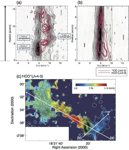
Figure 3: (a) Position-velocity diagrams of the ${\rm{}^{12}CO}$ ($J=3-2$) (black) and ${\rm HCO^{+}}$ ($J=4-3$) (red) emission lines taken along the cut labeled (a) in panel (c). (b) Same as panel (a), but for the other cut in panel (c). Contours in the position-velocity diagrams are drawn at 0.4, 0.8, 1, 2, 4, 8, 10, 20, 30, and 40 K for the ${\rm{}^{12}CO}$ emission line, and 0.2, 0.4, 1.0, 1.2, 1.4, 2.0, 2.2, and 2.4 K for the ${\rm HCO^{+}}$ emission line. (c) Mean velocity map of the ${\rm HCO^{+}}$ emission line over the velocity range $3.0\leqq V_{\rm LSR}\leqq 11.5$ km s${}^{-1}\,$. Contours represent the ${\rm HCO^{+}}$ integrated intensity map same as in Figure 1(b).

Figure 1 (b) shows the ${\rm HCO^{+}}$ ($J=4-3$) intensity distribution integrated over the velocity range $3.0\leqq V_{\rm LSR}\leqq 11.4$ km s${}^{-1}\,$superposed on the Herschel SPIRE $250\,\micron$ image (colored in gray). The ${\rm HCO^{+}}$ distribution is well correlated with the dust distribution traced by the Herschel data and 1.2 mm continuum image obtained by Maury et al. (2011, see their Figure 3). It is noteworthy that the local peaks of the ${\rm HCO^{+}}$ map are coincident with or located close to massive dense clumps identified by Pirogov et al. (2013) through the 1.2 mm continuum observations, although they mapped only a half of the area of our map. We found that the intense ${\rm HCO^{+}}$ emission is seen mainly in two parts in the map: One is the arc-shaped structure in the south-west part, and the other is the filamentary structure in the north-east part. The central part of the cluster including IRS 1A South ionizing the H ii region is located in between the two parts. As seen in Figure 1 (b), YSOs are distributed around the dense gas traced in ${\rm HCO^{+}}$ , suggesting that the sources were formed therein. The ${\rm HCO^{+}}$ map also shows that there is less dense gas around IRS 5, though several Class 0/I sources or starless cores have been detected there.

We did not detect the CCS ($J_{N}$=4${}_{3}-3_{2}$) emission in W40 at the present sensitivity. The CCS molecule is known to be more abundant in an earlier stage of chemical evolution (e.g., Suzuki et al., 1992; Hirota et al., 2009; Shimoikura et al., 2012). It is interesting to note that the Serpens South cloud located only $\sim 20\arcmin$ to the west of W40 exhibits strong CCS emission ($T_{\rm mb}\gtrsim 2$ K) as reported by Nakamura et al. (2014). They estimated the column density and fractional abundance of CCS to be $N$(CCS)$\simeq 1\times 10^{14}$ cm^-2 and $f$(CCS)$=10^{-10}-10^{-9}$ in the Serpens South cloud. From the noise level of our CCS data, we estimate the upper limits of $N$(CCS) and $f$(CCS) to be $\sim 1.1\times 10^{13}$ cm^-2 and $\sim 10^{-9.25}$ at the intensity peak position of the HCO⁺ emission in W40, respectively (see Appendix A). These values infer that $N$(CCS) in W40 is likely to be an order of magnitude smaller than in the Serpens South cloud, which can be the cause of the non-detection of the emission line. The upper limit of $f$(CCS) is comparable to the fractional abundance in the Serpens South cloud, suggesting that W40 may be more evolved (or at a similar stage at most) in terms of the chemical reaction time.

The velocity field of W40 shows a great complexity. Figure 2 displays the velocity channel maps of the ${\rm{}^{12}CO}$ and ${\rm HCO^{+}}$ emission lines with a velocity interval of 0.4 km s${}^{-1}\,$. The ${\rm{}^{12}CO}$ emission is significantly detected in two velocity ranges: One is the range $3\lesssim V_{\rm LSR}\lesssim 6$ km s${}^{-1}\,$and the other is the range $9\lesssim V_{\rm LSR}\lesssim 12$ km s${}^{-1}\,$. The ${\rm{}^{12}CO}$ emission is weak in the range $6\lesssim V_{\rm LSR}\lesssim 9$ km s${}^{-1}\,$where the ${\rm HCO^{+}}$ emission is prominent. This indicates that there is a velocity component at $V_{\rm LSR}$$\,\simeq 7$ km s${}^{-1}\,$, and the optically thick ${\rm{}^{12}CO}$ emission line is heavily self-absorbed while the optically thinner ${\rm HCO^{+}}$ emission appears as emission, which is obvious in the position-velocity (PV) diagrams shown in Figures 3 (a) and (b) together with the intensity-weighted mean velocity map of the ${\rm HCO^{+}}$ emission in Figure 3 (c). Note that, in addition to the velocity component at $\sim 7$ km s${}^{-1}\,$, there are also distinct components at $\sim 5$ and $\sim 10$ km s${}^{-1}\,$detected in ${\rm HCO^{+}}$ just around the H ii region. In the next subsection, we discuss the details of the velocity structures of the observed region.

3.2 Four Velocity Components

A careful inspection of the ${\rm{}^{12}CO}$ and ${\rm HCO^{+}}$ data infers that the observed region consists of at least four velocity components at $V_{\rm LSR}\simeq 3$, 5, 7, and 10 km s${}^{-1}\,$. As summarized in Table 1, the $\sim 7$ km s${}^{-1}\,$component represents the systemic velocity of the entire W40 region, and the $\sim 5$ and $\sim 10$ km s${}^{-1}\,$components are likely to originate from dense gas located along the expanding shell of the H ii region. The dense gas corresponds to Clump 1 ($\sim 5$ km s${}^{-1}\,$) and Clumps 5 and 6 ($\sim 10$ km s${}^{-1}\,$) detected in ${\rm HCO^{+}}$ that we will describe in Sections 3.5 and 3.6. The $\sim 3$ km s${}^{-1}\,$component is weak and shows up in a very limited region, and it might be unrelated to W40. As explained in the following, the four velocity components can be recognized in the ${\rm{}^{12}CO}$ and ${\rm HCO^{+}}$ spectra.

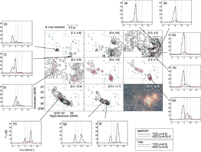
Figure 4: Channel maps of the ${\rm{}^{12}CO}$ (black contours) and ${\rm HCO^{+}}$ (red contours) emission lines in the velocity range $1.3\leqq V_{\rm LSR}\leqq 13.0$ with the 1.3 km s${}^{-1}\,$step. The velocity range in units of km s${}^{-1}\,$used for the integration is indicated in the top right corner of each panel. The lowest contours and the contour intervals are 5 K km s${}^{-1}\,$for the ${\rm{}^{12}CO}$ maps, and 1 K km s${}^{-1}\,$for the ${\rm HCO^{+}}$ maps. The 2MASS three-band composite image ($JHK$s) is overlaid in the last panel. The symbols for the YSOs are the same as in Figure 1. Representative ${\rm{}^{12}CO}$ (black lines) and ${\rm HCO^{+}}$ (red lines) spectra taken at some positions are also shown in panels (a) to (k). The ${\rm HCO^{+}}$ spectra are scaled up by a factor 2. The vertical broken lines indicate the typical velocities of the three components at $V_{\rm LSR}\simeq$5 km s${}^{-1}\,$, 7 km s${}^{-1}\,$, and 10 km s${}^{-1}\,$in Table 1.

In Figure 4, we show examples of the ${\rm{}^{12}CO}$ and ${\rm HCO^{+}}$ spectra observed at some positions mainly around the YSOs together with the velocity channel maps with a coarser velocity interval (1.3 km s${}^{-1}\,$) than Figure 2. The four components can be seen in some of the spectra. For example, the spectra in panels (a)–(c) sampled in the west of the H ii region consist only of the $\sim 5$ km s${}^{-1}\,$component, and those in panels (f) and (g) sampled in the south of the H ii region exhibit the $\sim 10$ km s${}^{-1}\,$component as well. Note that the $\sim 5$ and $\sim 10$ km s${}^{-1}\,$components are detected both in ${\rm{}^{12}CO}$ and ${\rm HCO^{+}}$ only around the H ii region. In addition, the ${\rm HCO^{+}}$ spectra in panels (e) and (i) consist of the $\sim 7$ km s${}^{-1}\,$component. The $\sim 3$ km s${}^{-1}\,$component is detected both in ${\rm{}^{12}CO}$ and ${\rm HCO^{+}}$ and is seen only around the positions shown in panels (j) and (k).

Compared with the 2MASS image in Figure 4, the $\sim 5$ and $\sim 10$ km s${}^{-1}\,$components exhibit intense ${\rm{}^{12}CO}$ emission, and they are likely to delineate the expanding shell around the H ii region. The $\sim 7$ km s${}^{-1}\,$component is well detected in ${\rm HCO^{+}}$ and is likely to represent the systemic velocity of the entire W40 region. As mentioned earlier, the absence of the intense ${\rm{}^{12}CO}$ emission for the $\sim 7$ km s${}^{-1}\,$component indicates that there is a large amount of cold gas in the foreground of the H ii region, which should cause the heavy absorption in ${\rm{}^{12}CO}$ around this velocity. Actually, the ${\rm{}^{12}CO}$ emission line over the velocity range $6-9$ km s${}^{-1}\,$have a brightness temperature of only $T_{\rm mb}\simeq 2$ K while the optically thinner ${\rm HCO^{+}}$ emission line is brighter (up to $\sim 8$ K) as seen in Figure 4 (e).

The above results are consistent with those obtained through earlier observations (e.g., Crutcher, 1977; Pirogov et al., 2013). Molecular observations done by Pirogov et al. (2013) covers the arc-shaped structure just around the H ii region, and they detected the two velocity components at $\sim 5$ and $\sim 7.5$ km s${}^{-1}\,$. Crutcher (1977) made ${\rm{}^{12}CO}$ $(J=1-0)$ observations with a lower angular resolution (HPBW$=2\farcm 6$), and they detected the ${\rm{}^{12}CO}$ emission at $\sim 5$ and $\sim 10$ km s${}^{-1}\,$. The author also found an absorption line at $\sim 7$ km s${}^{-1}\,$in the OH spectra obtained by additional observations with the NRAO 43 m telescope (HPBW$=18\arcmin$). Based on these data, Crutcher (1977) concluded that W40 has a single component with a peak velocity at $V_{\rm LSR}\simeq 7$ km s${}^{-1}\,$, which is extended in the wide velocity range $3-12$ km s${}^{-1}\,$and is self-absorbed at around 7 km s${}^{-1}\,$by colder gas in the foreground. We agree with their interpretation that W40 is surrounded by the $\sim 7$ km s${}^{-1}\,$component. In addition, we found the existence of two other velocity components at $\sim 5$ and $\sim 10$ km s${}^{-1}\,$around the H ii region, probably originating from the dense gas located along the expanding shell, which are detected both in ${\rm{}^{12}CO}$ ($J=3-2$) and ${\rm HCO^{+}}$ ($J=4-3$) as seen in the PV diagram in Figure 3 as well as in the spectra in Figures 4 (b) and (f).

3.3 Search for Outflows

Looking at the ${\rm{}^{12}CO}$ spectra in Figure 4, there are some cases in which high velocity wings are obviously seen in spite of the huge complexity in the velocity field. For example, the ${\rm{}^{12}CO}$ spectrum in Figure 4 (a) exhibits a blue-shifted wing at $V_{\rm LSR}$$\,\leq 3$ km s${}^{-1}\,$, and the one in Figure 4 (g) exhibits a red-shifted wing at $V_{\rm LSR}$$\,\geq 12$ km s${}^{-1}\,$. These wings are very likely to be tracing real high velocity gas, not mere Gaussian tails of the intense ${\rm{}^{12}CO}$ spectra of the $\sim 5$ and $\sim 10$ km s${}^{-1}\,$components. As detailed in the Appendix B, most of the ${\rm{}^{12}CO}$ spectra in the observed region can be well fitted by simple Gaussian functions except for the apparent high velocity wings as seen in Figure 4 (a) and (g).

Because the high velocity wings are often seen in the ${\rm{}^{12}CO}$ spectra along the dense condensations traced in ${\rm HCO^{+}}$ both around the H ii region and the filamentary structure, we suggest that they are either the high velocity gas blown away by the expansion of the H ii region or the outflowing gas driven by YSOs forming in the dense condensations. At the moment, there is no way to distinguish these two effects reliably only with the present dataset, and both of them should be actually at play. Modeling the expected signature of instabilities in high velocity gas from H ii region expansion is beyond the scope of the current study. For the purpose of this study, we interpret apparent high velocity wings on the principal velocity components of ${\rm{}^{12}CO}$ as evidence of potential “candidate” outflows from YSOs and derive their parameters accordingly. Though a certain fraction of the high velocity wings can be due to the expansion of the H ii region, there are some high velocity wings found in the vicinity of YSOs (e.g., “B2” and “R2” in the following) including the one located away from the H ii region (e.g., “R4”) which are likely to be promising outflows from YSOs.

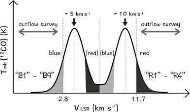
Figure 5: Schematic illustration to search for the high velocity wings of outflows in the ${\rm{}^{12}CO}$ spectra. In the W40 region, there are three main velocity components at $V_{\rm LSR}\simeq 5$, 7, 10 km s${}^{-1}\,$(Table 1) , but the heavy absorption by the $\sim 7$ km s${}^{-1}\,$component precludes the detection of the high velocity wings over the velocity range $6\lesssim V_{\rm LSR}\lesssim 9$ km s${}^{-1}\,$. We therefore searched for the ${\rm{}^{12}CO}$ emission in the velocity ranges $-3.2\leqq V_{\rm LSR}\leqq 2.8$ km s${}^{-1}\,$and $11.7\leqq V_{\rm LSR}\leqq 14.5$ km s${}^{-1}\,$to find candidates of the blue- and red-shifted wings of the outflows, respectively. The ${\rm{}^{12}CO}$ intensity integrated over these velocity ranges are shown by the blue and red solid contours in Figure 6. Outflow candidates originating from the $\sim 5$ km s${}^{-1}\,$and $\sim 10$ km s${}^{-1}\,$components may show symmetric wing components, and so, for a reference, we further investigated possible wing components contained in the velocity ranges $5.7\leqq V_{\rm LSR}\leqq 8.4$ km s${}^{-1}\,$and $8.5\leqq V_{\rm LSR}\leqq 9.2$ km s${}^{-1}\,$. The ${\rm{}^{12}CO}$ intensities integrated over these velocity ranges are shown by the red and blue broken contours in Figure 6.

Since the dense gas consists of the $\sim 5$ km s${}^{-1}\,$, $\sim 7$ km s${}^{-1}\,$, and $\sim 10$ km s${}^{-1}\,$components, we searched for outflow candidates blowing out from these components. For the $\sim$3 km s${}^{-1}\,$component, we did not find any high velocity wings in the ${\rm{}^{12}CO}$ spectra, and thus we disregarded this component. In order to carry out a systematic search for outflows, we set constant velocity ranges to find high velocity wings in the ${\rm{}^{12}CO}$ spectra. As illustrated in Figure 5, we decided to use the velocity ranges $-3.2\leqq V_{\rm LSR}\leqq 2.8$ km s${}^{-1}\,$and $11.7\leqq V_{\rm LSR}\leqq 14.5$ km s${}^{-1}\,$for the blue- and red-shifted high velocity wings of outflows, respectively. Basically, we can carry out a reliable search for outflow candidates in ${\rm{}^{12}CO}$ only in these velocity ranges, because the heavy absorption by the $\sim 7$ km s${}^{-1}\,$component precludes the detection of the faint wing emission over the range $6\lesssim V_{\rm LSR}\lesssim 9$ km s${}^{-1}\,$. However, for a reference, we will also investigate wing emission possibly associated with the $\sim 5$ and $\sim 10$ km s${}^{-1}\,$components in the range $5.7\leqq V_{\rm LSR}\leqq 8.4$ km s${}^{-1}\,$and $8.5\leqq V_{\rm LSR}\leqq 9.2$ km s${}^{-1}\,$, because, in the vicinity of the H ii region, Zhu et al. (2006) found a bipolar outflow associated with the $\sim 5$ km s${}^{-1}\,$component, though we now realize that its red-shifted wing emission should be contaminated by the heavy absorption.

Figure 6 shows the ${\rm{}^{12}CO}$ intensity distributions integrated over the velocity ranges mentioned in the above. The overall distributions of the high velocity gas in the figures show a great complexity similar to what has been reported for the Circinus cloud where the complex outflow lobes are found to be a mixture of some smaller outflows (e.g., Dobashi et al., 1998; Bally et al., 1999; Shimoikura & Dobashi, 2011), which is likely the case also for W40. In addition, the ${\rm{}^{12}CO}$ distributions in the figures are contaminated by some distinct velocity components (at $V_{\rm LSR}\simeq 3$ km s${}^{-1}\,$) unrelated to the outflows.

The ${\rm{}^{12}CO}$ distributions on the sky are too complex to separate them reliably into single outflow candidates only from the present dataset. In this paper, we thus decided to pick up the local peaks in the ${\rm{}^{12}CO}$ intensity map in Figure 6 if they are not due to the distinct velocity components but are very likely due to outflows showing a wing-like feature in the ${\rm{}^{12}CO}$ spectra. As a result, we found 13 local peaks as indicated in Figure 6. For simplicity, we will regard each of the 13 local peaks as the peak position of a single high velocity lobe and we will consider them to be candidates of outflows in W40. There are nine blue lobes and four red lobes. As summarized in Table 2, we call the blue lobes “B1”–“B9”, and the red lobes “R1”–“R4”.

To measure some physical properties, we defined the surface area of the outflow lobes $S_{\rm lobe}$ at the 1.2 K km s${}^{-1}\,$(corresponding to the $\simeq 9\sigma$ noise level) contour level. In the case that two or more lobes are attached to each other at this threshold value, we divided them into single lobes at the valley in the contour maps of the ${\rm{}^{12}CO}$ intensity (Figure 6). We also attempted to find driving sources of the outflow lobes. It is however also difficult to identify the driving sources reliably, and thus we simply picked up YSOs located within $S_{\rm lobe}$ defined in the above as possible candidates for the driving sources. There are nine outflow candidates (B1, B2, B4, B6, B7, B8, R1, R2, and R4) with at least one candidate of the driving source, and there are four outflow candidates (B3, B5, B9, and R3) which could not be assigned to any known sources.

We summarize the main features of the outflow lobes as follows.

Blue lobes: Blue lobes are seen mainly around the H ii region. A candidate for the driving source of B1 is 1.2 mm source, which is found and classified as “starless” by Maury et al. (2011). A jet-like blue lobes B2 and B3 elongated in the East-West direction are clearly seen in Figure 6. B3 is the largest lobe located close to IRS 5. Multiple blue lobes B4–B8 are located to the south of the H ii region. B9 is a small lobe found in the filament structure. B1–B8 correspond to an outflow discovered by Zhu et al. (2006, see their Figure 3) with lower angular resolution ($80\arcsec$), which is resolved into smaller multiple possible outflows in our map.

Red lobes: Two red lobes R1 and R2 are detected in the vicinity of IRS 1A South, suggesting that these outflow candidates possibly originate in the cluster. Candidates of driving sources for these lobes are classified as Class I protostars (Mallick et al., 2013). The lobes R3 and R4 are found in the filament structure.

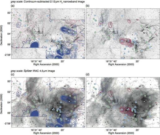
Figure 7: Comparison of the CO outflow candidates (contour) and other emission lines (gray scale). (a) Locations of blue lobes of the outflow candidates (same as in Figure 6(a)) overlaid with the continuum-subtracted 2.12 $\micron$ H₂ narrowband image obtained by Mallick et al. (2013). (b) Same as (a), but for red lobes (same as in Figure 6(b)). (c) Locations of blue lobes of the outflow candidates overlaid with the Spitzer IRAC 4.5 $\micron$ image. (d) Same as (c), but for red lobes. The symbols for the YSOs are the same as in Figure 1.

Finally, in Figure 7(a) and (b), we compared the distributions of the outflow candidates with the continuum-subtracted 2.12 $\micron$ H₂ narrowband image obtained by Mallick et al. (2013) to search for the possible counterparts of the CO outflow lobes. We also compared our map with the Spitzer IRAC 4.5 $\micron$ image in Figure 7(c) and (d) to see whether vibrationally excited CO emission is detected around the outflow candidates. However, we could not identify clear counterparts corresponding to the outflow lobes in these images, though there are some near/mid-infrared nebulosity in the vicinity.

According to the Herschel map (the left panel of Figure 1 (b)), the H ii region is apparently expanding into the surrounding medium, and some of the identified lobes (i.e., B2, B3, R1, and R2) are located in less dense regions at the edge of the H ii region. Furthermore, these lobes are associated with the $\sim 5$ and $\sim 10$ km s${}^{-1}\,$components which are likely to represent the expanding velocity of the shell (see Section 3.6). For the lobes found just around the H ii region, we cannot distinguish if the observed high velocity gas is due to real outflows from YSOs or is merely tracing the expanding shell. In addition to the above possibility, we should also note that some of the identified lobes might not originate from a single YSO (see Figure 6), but originate from the cluster in the H ii region. All of these ambiguities arise from the complex velocity filed in W40, especially the heavy absorption by the $\sim 7$ km s${}^{-1}\,$component. In this paper, we will regard the 13 blue- and red-shifted high velocity lobes to be candidates of outflows in this region and will estimate some outflow parameters in Section 3.4.

3.4 Properties of Outflow Candidates

In order to estimate the masses of the outflow candidates, we assumed that the ${\rm{}^{12}CO}$ molecules are in the local thermal equilibrium (LTE) and also that the ${\rm{}^{12}CO}$ emission is optically thin at all wing velocities to calculate the column densities in the outflow lobes for a uniform excitation temperature of $T_{\rm ex}=30$ K. We then estimated the mass, momentum, and energy of the outflow lobes. Details of the calculations of the physical parameters are described in Appendix C, and the results are summarized in Table 2.

Zhu et al. (2006) suggested a total mass of 0.48 $M_{\sun}$ for the blue lobe of the outflow they found which corresponds to our B1 to B8, on the assumption of a distance of 600 pc and a mean molecular weight of 2.72 (cf., we assumed 500 pc and 2.4, respectively). The sum of the corresponding blue lobes in our Table 2 amounts only to $\sim 0.11$ $M_{\sun}$ which would be rescaled to $\sim 0.18$ $M_{\sun}$ for the same assumptions as theirs. The difference between their and our estimates is mainly due to the contamination of the distinct velocity component at $V_{\rm LSR}\simeq 3$ km s${}^{-1}\,$(see Section 3.2) which was not resolved in their observations, and also due to the fact that we defined the surface area of the outflow lobes at a rather high threshold value of 1.2 K km s${}^{-1}\,$(see Section 3.3).

As seen in the 8th column of Table 2, we found that the masses of the individual lobes are in the range from $\sim 0.001$ $M_{\sun}$ to $\sim 0.03$ $M_{\sun}$. The YSOs that can be the possible driving sources of these outflow candidates have bolometric luminosities $L_{\rm bol}\simeq 4.2-6.6\,L_{\sun}$ (Maury et al., 2011, see their Table 1). According to a statistical study of outflows by Wu et al. (2004), outflows associated with low-mass YSOs with $L_{\rm bol}\simeq 1-10\,L_{\sun}$ have a mass range of $0.01$ $M_{\sun}$ to a few $M_{\sun}$. The masses of outflow candidates we found in W40 are much smaller than the average mass of outflows associated with low-mass YSOs, and are close to the lower end in the plots of the outflow masses versus the bolometric luminosity of the driving sources reported by Wu et al. (2004) (see their Figure 5).

Here we estimate the possible errors in the derived parameters caused by our assumptions. First, we assumed the constant excitation temperature $T_{\rm ex}=30$ K. An error arising from this assumption should be small, because the outflow masses are insensitive to $T_{\rm ex}$, and they would fluctuate only by $\sim$20$\%$ at most within the variation of $T_{\rm ex}$ in the mapped region ($20<T_{\rm ex}<65$ K). Second, we assumed that wing components in the ${\rm{}^{12}CO}$ ($J=3-2$) emission line are optically thin ($\tau\ll 1$), but they might be moderately optically thick. For example, Dunham et al. (2014) investigated 17 outflows associated with low mass stars with the ${\rm{}^{12}CO}$ ($J=3-2$) and ¹³CO ($J=3-2$) emission lines, and found the optical depths of the ${\rm{}^{12}CO}$ ($J=3-2$) emission line varies in the range $\tau\simeq 1-10$ with an average value of $\sim 2.8$. If we adopt their average value, the inverse of the escape probability in Equation (C3) would be $\beta^{-1}=3.0$. This infers that our optically thin assumption may cause an underestimation in the mass estimate by a factor of a few. Finally, it is important to remark that the parameter $V_{\rm wing}$ (i.e., the velocity range exhibiting the high velocity wings) in Equations (C4)–(C7) should be highly underestimated because of the heavy absorption in the velocity range $6\lesssim V_{\rm LSR}\lesssim 9$ km s${}^{-1}\,$, and hence our estimate for the mass, energy, and momentum of the outflows should be highly underestimated.

To summarize our outflows survey, we found that 13 candidates of outflow lobes showing wing-like emission in the ${\rm{}^{12}CO}$ spectra. However, we should note that our estimates of the outflow parameters such as the mass, momentum, and energy should give only the lower limits to the actual values mainly because of the heavy absorption at $\sim 7$ km s${}^{-1}\,$and the optically thin assumption. For most of the outflow candidates identified, we cannot even pair red and blue lobes, because of their complex distributions (e.g., Arce et al., 2010; Offner et al., 2011; Bradshaw et al., 2015).

3.5 Clumps Detected in HCO⁺

The ${\rm HCO^{+}}$ ($J=4-3$) emission line is a good tracer of cold dense gas for its high critical density $>10^{6}$ cm^-3(e.g., Girart et al., 2000). As stated in Section 3.2, the radial velocities of the ${\rm HCO^{+}}$ emission can be classified to the three velocity components at $\sim 5$, 7, and 10 km s${}^{-1}\,$in Table 1, and they can be mostly well separated at $V_{\rm LSR}=$6.0 and 9.0 km s${}^{-1}\,$. We show the ${\rm HCO^{+}}$ integrated intensity maps divided at these velocities in Figure 8. In order to investigate physical properties of the dense gas detected in ${\rm HCO^{+}}$ , we will define clumps based on these maps. We will regard a condensation enclosed by the lowest contours (1 K km s${}^{-1}\,$$\simeq 6\,\sigma$) having the peak integrated intensity greater than 2 K km s${}^{-1}\,$in each map as one clump. There are five condensations satisfying the criteria. However, a large condensation in the $6\leqq V_{\rm LSR}\leqq 9$ km s${}^{-1}\,$range exhibits two slightly different velocity components by $\sim 1$ km s${}^{-1}\,$, and thus we divided them into two at the boundary of the two velocity components as labelled Clumps 3 and 4 in Figure 8. As a result, we identified six clumps in the ${\rm HCO^{+}}$ data. We show the ${\rm HCO^{+}}$ spectra sampled at their peak positions in Figure 8, and also show the line parameters (i.e., the peak brightness temperature, line width, and peak velocity) obtained by fitting the spectra with a single Gaussian function in Table 4.

Based on the ${\rm HCO^{+}}$ data, we will derive molecular masses of the clumps on the assumption of the LTE using Equations (C2) and (C3) for $X=$HCO⁺ (see Appendix C). According to JPL Catalog and Splatalogue, the constants $B_{0}$, $\mu$, and $E_{u}$ are 44.5944 GHz, 3.888 debye, and 29.7490 cm^-1, respectively, for the ${\rm HCO^{+}}$ ($J=4-3$) emission line. We list these constants in Table 3.

In order to derive the mass of the clumps, we estimated $T_{\rm ex}$ for ${\rm HCO^{+}}$ comparing our ${\rm HCO^{+}}$ ($J=4-3$) data with the ${\rm HCO^{+}}$ $(J=1-0)$ data measured by Pirogov et al. (2013) toward some limited positions (see their Table 4). For these positions, we smoothed our ${\rm HCO^{+}}$ ($J=4-3$) spectra to the same angular resolution as the ${\rm HCO^{+}}$ $(J=1-0)$ spectra ($\sim 45\arcsec$), and applied the non-LTE radiative transfer code RADEX (van der Tak et al., 2007). Results of the analyses infer $T_{\rm ex}\gtrsim 30$ K to reproduce the hydrogen number density $n({\rm H}_{2})\simeq 1\times 10^{6}$ cm^-3 found by Pirogov et al. (2013) for these positions. This value of $T_{\rm ex}$ is consistent with the temperatures of dense gas around the H ii region measured by Pirogov et al. (2013) using NH₃ and dust continuum data ($16-40$ K, see their Table 7). In this paper, we therefore adopt $T_{\rm ex}=30$ K throughout the observed region.

If we assume that the emission line is optically thin ($\tau\ll 1$), the ${\rm HCO^{+}}$ column density can be derived by the following equation for $T_{\rm ex}=30$ K,

$$N_{\rm HCO^{+}}=4.53\times 10^{11}\int_{V_{\rm range}}T_{\rm mb}^{\rm HCO^{+}}(v)~{}{\rm d}v~{}~{}~{}~{}{\rm cm^{-2}}$$ (1)

where the term $\int T_{\rm mb}^{\rm HCO^{+}}(v)~{}{\rm d}v$ is in units of K km s${}^{-1}\,$. The velocity range for the integration $V_{\rm range}$ is the same as shown in Figure 8, i.e., $3\leqq V_{\rm LSR}\leqq 6$ km s${}^{-1}\,$, $6\leqq V_{\rm LSR}\leqq 9$ km s${}^{-1}\,$, and $9\leqq V_{\rm LSR}\leqq 12$ km s${}^{-1}\,$for clumps at $\sim 5$ km s${}^{-1}\,$(Clump 1), $\sim 7$ km s${}^{-1}\,$(Clumps 2–4), and $\sim 10$ km s${}^{-1}\,$(Clumps 5 and 6), respectively.

Assuming the fractional ${\rm HCO^{+}}$ abundance ratio to be $N_{\rm HCO^{+}}/N_{\rm H_{2}}=2.5\times 10^{-10}$ found by Pirogov et al. (2013) through comparison of the ${\rm HCO^{+}}$ ($J=1-0$) emission line and 1.2 mm continuum data toward our Clump 1, the total mass of the clumps can be estimated by the following equation,

$$M_{\rm clump}=2.96\times 10^{-6}\,D^{2}{\int_{S_{\rm clump}}\int_{V_{\rm range}}T_{\rm mb}^{\rm HCO^{+}}}(v){\rm d}v{\rm d}S~{}~{}~{}M_{\sun}$$ (2)

where the term ${\int\int T_{\rm mb}^{\rm HCO^{+}}}{\rm d}v{\rm d}S$ is in units of K km s${}^{-1}\,$arcmin² and $D$ is the distance to the clumps in units of pc ($D=500$ pc for W40). We defined $S_{\rm clump}$ is the surface area of the clump at the 1 K km s${}^{-1}\,$contour level.

Using Equations (1) and (2), we estimated the total mass of the clumps. The results are presented in Table 4. As seen in the table, the identified clumps have a masses ranging from $\sim 2$ to 26 $M_{\sun}$ with a mean value of $\sim 12$ $M_{\sun}$.

Here, we should note that our mass estimates depend on the adopted $T_{\rm ex}$. The derived masses should increase for lower $T_{\rm ex}$, and they would change by $\sim 50$ $\%$ at most if $T_{\rm ex}$ varies in the range $16-40$ K as measured by Pirogov et al. (2013).

Pirogov et al. (2013) suggested a total mass of 8.1 $M_{\sun}$ (the sum of the masses of their clumps 2 and 3) for a part of our Clump 2 from the 1.2 mm continuum data. We estimate the mass contained in the same area measured by Pirogov et al. to be 9 $M_{\sun}$. The mass derived from our ${\rm HCO^{+}}$ data is therefore in close agreement with that derived by Pirogov et al. (2013). However, on a larger scale, Maury et al. (2011) suggested a much larger mass than our estimate. They estimated the total mass of a larger region equivalent to our entire observed area to be 310 $M_{\sun}$ through the Herschel column density map. They assumed a distance of 260 pc, and thus the mass should be rescaled to $\sim 1150\,M_{\sun}$ for our assumed distance (500 pc). We obtain only $\sim 110\,M_{\sun}$ as the total mass of the observed region, which is only $10\%$ of their mass. This is probably due to the fact that the dust emission (detected by Herschel) traces all of the dust along the line-of-sight, while ${\rm HCO^{+}}$ traces only very high density regions because of its high critical density ($>10^{6}$ cm^-3). Moreover, as suggested by Girart et al. (2000), ${\rm HCO^{+}}$ ($J=4-3$) is not likely to be thermalized, and therefore the masses derived here are lower limits.

Finally, we attempt to find the possible association between the identified clumps and the outflow lobes found in the previous subsections, though it is difficult to establish their definite association because of the enormous complexity in the velocity field for which we cannot identify even their driving sources reliably. Here, we regard that the clumps and the outflow lobes are associated if their surface areas overlap each other. All of the outflow lobes except for B1 and B3 have an overlap with one or more clumps. We will regard that B1 and B3 are associated with Clump 1, because weak ${\rm HCO^{+}}$ emission is extending from this clump toward these outflow lobes. We also checked the systemic velocity $V_{\rm sys}$ for each of the lobes (see Appendix C and the 6th column of Table 2). For B7 and B8, these $V_{\rm sys}$ are close to the radial velocity of Clump 2 and we will regard these lobes are associated with Clump 2. The results summarized in the last column in Table 4.

Comparing the identified clumps with the distributions of the YSOs in Figure 8, It is interesting to note that some of the ${\rm HCO^{+}}$ clumps (e.g., Clump 1 and Clump 4) are associated with Class 0/I sources at their peak positions. Moreover, the clumps associated with the outflow lobes tend to have broader line widths (see Table 4), suggesting that the outflow lobes are influencing on the kinematics of the parent clumps. Nakamura & Li (2007) investigated theoretically the complex interplay between outflows induced by star formation and turbulence of the parent clumps, and showed that outflows should play a significant role in altering the star-forming environments. The energy and momentum of the outflows found in this study appear too small to give significant influence on the parent clumps, but again, we should note that our estimates for the outflow parameters may suffer from a large uncertainty.

3.6 Three-Dimensional Model of W40

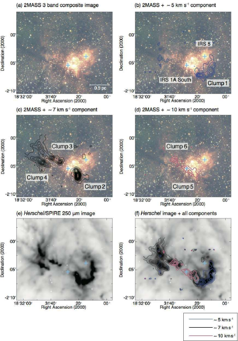
Figure 9: Distributions of dense gas traced in ${\rm HCO^{+}}$ and dust revealed by 2MASS and Herschel. Panel (a) displays the three-colors ($JHK$s) composite image of 2MASS. Panels (b)–(d) display the same 2MASS image, but overlaid with the ${\rm HCO^{+}}$ intensity maps (contours) integrated over the velocity range $3\leqq V_{\rm LSR}\leqq 6$ km s${}^{-1}\,$(blue contours), $6\leqq V_{\rm LSR}\leqq 9$ km s${}^{-1}\,$(black contours), and $9\leqq V_{\rm LSR}\leqq 12$ km s${}^{-1}\,$(red contours), respectively. Panel (e) displays the Herschel $250\,\micron$ image. Panel (d) displays the same Herschel image, but overlaid with the ${\rm HCO^{+}}$ intensity maps. Blue plus signs denote the locations of IRS 1A South and IRS 5.

Here, we discuss the locations of the identified clumps relative to the H ii region and propose an updated three-dimensional model of W40. Previous studies suggested that the H ii region lies on the edge of a large molecular cloud in a support of the blister model (e.g., Zeilik & Lada, 1978; Vallee, 1987). More recently, Herschel revealed the total dust distribution in W40 (e.g., André et al., 2010; Könyves et al., 2010). We show the 250 $\micron$ image by Herschel and the three-colors ($JHK$s) composite image of 2MASS in Figure 9 overlaid with our ${\rm HCO^{+}}$ channel maps ($\sim 5$ km s${}^{-1}\,$, $\sim 7$ km s${}^{-1}\,$, and $\sim 10$ km s${}^{-1}\,$). Morphological coincidence between the molecular gas and the dust seen in the far-infrared emission (Herschel) and in the near-infrared absorption (2MASS) is obvious. It is noteworthy that Clumps 3 and 4 show up in the 2MASS image in the absorption, indicating that these clumps are located in the foreground of the H ii region.

Among the four velocity components summarized in Table 1, the $\sim 7$ km s${}^{-1}\,$component is the primary component of molecular gas around W40. Our Clumps 2–4 exhibit this velocity in ${\rm HCO^{+}}$ . As seen in the PV diagram in Figure 3, there is a heavy absorption feature in the ${\rm{}^{12}CO}$ emission over the velocity range $6\lesssim V_{\rm LSR}\lesssim 9$ km s${}^{-1}\,$. Nakamura et al. (2011) have shown that the same absorption feature in ${\rm{}^{12}CO}$ is clearly seen around the Serpens South molecular cloud ($\sim 20\arcmin$ to the west of W40) at the same velocity range. Dzib et al. (2010) measured the distance to Serpens Main to be approximately 415 pc through VLBI observations, which is much further than previously thought (e.g., 260 pc, Maury et al., 2011). On the other hand, the distance of W40 has not been determined precisely varying in the range 340–600 pc (e.g., Rodney & Reipurth, 2008; Kuhn et al., 2010; Shuping et al., 2012), and the W40 and Serpens South regions might be physically connected as suggested by some authors (e.g., Bontemps et al., 2010). A more likely explanation for the absorption is that a colder cloud, perhaps a part of the envelope surrounding both of the W40 and Serpens regions, lies in the foreground. We thus regard that Clumps 3 and 4 are a part of the larger cloud surrounding these regions, and that they are located in the foreground of W40.

In the ${\rm HCO^{+}}$ data, the other velocity components at $\sim 5$ and $\sim 10$ km s${}^{-1}\,$are seen mostly around the H ii region. These components are very bright in ${\rm{}^{12}CO}$ ($T_{\rm mb}\gtrsim 40$ K), indicating that they are probably interacting with the H ii region being located close to the ionization front. This picture is consistent with the blister model suggested by Vallee (1987) in which the H ii region is expanding away from the dense molecular core located near the cloud surface. We will develop the picture suggested by Vallee (1987). The ionized gas associated with the H ii region is expanding not only outward but also into the molecular cloud pushing away the surrounding dense gas. In this interpretation, Clumps 1, 2, and 5 should be part of the expanding shell. It is noteworthy that these clumps have a radial velocity of $\sim 5$ km s${}^{-1}\,$, $\sim 7.5$ km s${}^{-1}\,$, and $\sim 10$ km s${}^{-1}\,$. This infers that they are the dense gas interacting with the H ii region being swept up by the expansion of the ionization front.

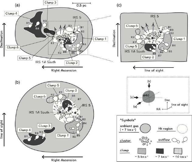
Figure 10: Schematic illustration of the proposed model for the three-dimensional geometry of the W40 region. As indicated in the box drawn by the broken line, panel (a) shows the view as is observed on the sky (e.g., see Figure 9(b)–(d)), and panel (b) shows the view observed from the declination axis orthogonal to the line-of-sight. Panel (c) shows the close-up view around the H ii region observed from the right ascension axis (Clumps 3 and 4 are not drawn). In the model, Clump 1 ($V_{\rm LSR}\simeq 5$ km s${}^{-1}\,$) is located on the near side of the expanding sphere of the H ii region, and Clumps 5 and 6 ($\sim 10$ km s${}^{-1}\,$) are located on the far side of the same sphere. Clumps 3 and 4 ($\sim 7$ km s${}^{-1}\,$) are located in the foreground of the H ii region.

On the basis of the above results and discussion, we suggest a three-dimensional model of the clump distributions in W40, which is summarized in the schematic illustration shown in Figure 10. In the following, we will discuss the locations of the individual clumps based on the ${\rm HCO^{+}}$ and ${\rm{}^{12}CO}$ data and on their appearance in the 2MASS image (Figure 9). The molecular data provide us the information on the velocity and temperature of the clumps, and the scattered light seen in the 2MASS image often infers the geometry between the clumps and the H ii region.

Clump 1: In the 2MASS image, this clump is located very close to the H ii region. The rim of the clump facing to the H ii region is bright, and the rest of the clump appears opaque (Figure 9 (b)). The ${\rm{}^{12}CO}$ emission from this clump is very intense ($\sim 53$ K, see Figure 4 (c)) with a radial velocity of $\sim 5$ km s${}^{-1}\,$which is blue-shifted by $\sim 2$ km s${}^{-1}\,$compared to the systemic velocity of the entire W40 region ($\sim 7$ km s${}^{-1}\,$). We thus suggest that the clump is located on the near side of the expanding sphere of the H ii region being heated and swept up toward us by the ionization front.

Clump 2: This clump is the brightest in ${\rm HCO^{+}}$ among all of the clumps ( $\sim 8$ K, see Table 4) with a high density of $n({\rm H_{2}})\gtrsim 10^{6}$ cm^-3 (Pirogov et al., 2013). This clump overlaps with Clump 1 on the sky, but they can be clearly separated in velocity. We cannot identify Clump 2 on the 2MASS image, but its counterpart can be recognized in the Herschel 250 $\micron$ image (see Figure 9(f)), suggesting that Clump 2 is located behind Clump 1. The radial velocity of Clump 2 is $\sim 7.6$ km s${}^{-1}\,$which is consistent with the systemic velocity, and thus the clump might be located in the ambient background gas apart from the H ii region. However, Pirogov et al. (2013) found a high kinetic temperature of 40 K for this clump based on the non-LTE modeling for the CS $(J=2-1)$ and $(J=5-4)$ emission lines (see their Table 7), suggesting that Clump 2 is probably in the vicinity of the H ii region. The above observational features would be naturally accounted for if we assume that the clump is interacting with the H ii region like in the case of Clump 1, being swept up toward the direction orthogonal to the line-of-sight, as illustrated in Figure 10 (c).

Clumps 3 and 4: These clumps are apart from the H ii region on the sky, and they can be easily identified in the 2MASS image as the opaque filaments (Figure 9 (c)). The peak velocities of the ${\rm HCO^{+}}$ emission line of Clump 3 is $\sim 8$ km s${}^{-1}\,$and that of Clump 4 is $\sim 7$ km s${}^{-1}\,$consistent with the systemic velocity of the W40 region. These observational facts indicate that they are located in the foreground of the H ii region as explained earlier. However, we should note that Clumps 3 consists of two well defined peaks, and one of them in the south-west appears as a small clump with the faint scattered light in the 2MASS image, not as the opaque region. This part might be separated from the other peak with a different location along the line-of-sight, though they are connected by the weak ${\rm HCO^{+}}$ emission.

Clump 5: This clump has a radial velocity of $\sim 10$ km s${}^{-1}\,$which is red shifted by $\sim 3$ km s${}^{-1}\,$from the systemic velocity. The clump is very bright in ${\rm{}^{12}CO}$ ($\sim 50$ K, see Figure 4 (f)), suggesting that the clump is interacting with the H ii region on the far side of the expanding sphere of the H ii region. The extent of Clump 5 coincides with the bright region in the 2MASS image around IRS 1A South (Figure 9 (d)), and we cannot recognize the shape traced in ${\rm HCO^{+}}$ in the image.

Clump 6: This clump is located between the two local peaks of Clump 3 (at $\sim$8 km s${}^{-1}\,$) on the sky, but it has a clearly different velocity ($\sim 9$ km s${}^{-1}\,$). There is a faint nebulosity around Clump 6 in the 2MASS image. This clump is located rather far from the H ii region on the sky, and it exhibits ${\rm{}^{12}CO}$ emission with a moderate brightness temperature of $\sim 30$ K (Figure 4 (h)). We cannot decide the location of this clump with a confidence, but we suggest that it may be located rather in the back of the H ii region because of its appearance in the 2MASS image as well as of its slightly red-shifted radial velocity compared to the systemic velocity.

As illustrated in Figure 10, Clumps 1, 2, and 5 are likely to be located just around the H ii region. They are probably dense gas being compressed by the expansion of the H ii region. It is interesting to note that 10 outflow lobes found in the ${\rm{}^{12}CO}$ data are likely to be associated with these clumps. This is suggestive of star formation triggered by the impact of expanding H ii region driven by nearby massive young stars, indicating that the sequential star formation (e.g., Elmegreen & Lada, 1977) is taking place in this region.

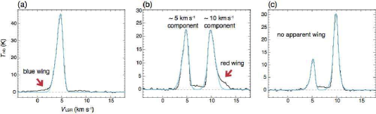
Figure 11: Examples of the Gaussian functions (blue lines) best fitting the observed ${\rm{}^{12}CO}$ emission lines (black lines) exhibiting (a) a blue-shifted high velocity wing associated with the $\sim 5$ km s${}^{-1}\,$component, (b) a red-shifted high velocity wing associated with the $\sim 10$ km s${}^{-1}\,$component, and (c) no apparent high velocity wing. Each of the $\sim 5$ and $\sim 10$ km s${}^{-1}\,$components is fitted with two Gaussian functions. The spectra in panels (a), (b), and (c) are the ${\rm{}^{12}CO}$ spectra shown in panels (a), (g), and (h) of Figure 4, respectively.

We also should note that three outflow lobes are likely to be associated with Clump 4 which is away from the H ii region. It could be possible that the clump will be another site of cluster formation in W40. According to the study of 11 young clusters in the S247, S252, and BFS52 regions including the Monkey Head nebulae (Shimoikura et al., 2013), four of the clusters actually consists of two or more smaller clusters with a separation of $\sim 1$ pc (e.g., see their Figure 11(c)). Such multiple cluster formation in a limited region may not be rare, because there are some other young clusters showing multiplicity (e.g., the S235 region, Kirsanova et al., 2014). Though the relation between Clump 4 and the H ii region is unclear, the dust distributions on a larger scale indicate that there are two outstanding condensations of dust around Clump 4 and the H ii region (e.g., see Figure 1(b)), suggesting that the W40 region might be a site of sequential cluster formation.

4 CONCLUSIONS

We have carried out ${\rm{}^{12}CO}$ ($J=3-2$) and ${\rm HCO^{+}}$ ($J=4-3$) observations around the H ii region W40 with the ASTE 10 m telescope and identified CO outflows and dense clumps in this region. We have also observed the region with molecular lines at 45 GHz such as SiO ($J=1-0$, $v=0$) and CCS ($J_{N}$=4${}_{3}-3_{2}$) using the 45 m telescope at NRO. We summarize the main conclusions of this paper in the following points (1)–(4):

(1) Intense ${\rm{}^{12}CO}$ (up to $T_{\rm mb}\simeq 50$ K) and ${\rm HCO^{+}}$ emission (up to $\sim 8$ K) lines were detected around the W40 H ii region. The velocity field in the region is highly complex, showing at least four distinct velocity components at $V_{\rm LSR}\simeq 3$, 5, 7, and 10 km s${}^{-1}\,$. The $\sim 7$ km s${}^{-1}\,$component represents the systemic velocity of the region which causes heavy absorption in the ${\rm{}^{12}CO}$ spectra over the velocity range $6\lesssim V_{\rm LSR}\lesssim 9$ km s${}^{-1}\,$. The $\sim 5$ and $\sim 10$ km s${}^{-1}\,$components exhibit high ${\rm{}^{12}CO}$ temperature ($\gtrsim 40$ K), and observed mainly around the H ii region. The $\sim 3$ km s${}^{-1}\,$component is faint, and might be unrelated to W40.

(2) The SiO, CCS, HC₃N, and HC₅N emission lines were not detected at the present sensitivity. We estimated the upper limits of the column density of CCS and its fractional abundance of W40 to be $\sim 1.1\times 10^{13}$ cm^-2 and $\sim 10^{-9.25}$, respectively.

(3) Based on the ${\rm{}^{12}CO}$ ($J=3-2$) data, we made a survey for molecular outflows over the observed region. We searched for high velocity outflow lobes in the velocity range $V_{\rm LSR}\leqq 2.8$ km s${}^{-1}\,$for the blue lobes and $V_{\rm LSR}\geqq 11.7$ km s${}^{-1}\,$for the red lobes. As a result, we identified nine candidates for the blue lobes and four candidates for the red lobes, and estimated the lower limits of physical parameters such as the mass, momentum, and energy. Though some of the identified lobes around the H ii regions (i.e., B2, B3, R1, and R2) might not be real outflows but merely tracing the high velocity gas of the expanding shell of the H ii region, it is difficult to distinguish the two phenomenon with the present dataset, because of the complex velocity field in W40.

(4) Based on the ${\rm HCO^{+}}$ ($J=4-3$) data, we identified six clumps and derived their physical properties such as the mass, radial velocities, and surface areas. We further discussed their locations relative to the H ii region, and suggested a three-dimensional model of their distributions.

Appendix A Derivation of the Column Density and the Fractional Abundance of CCS

We estimated the upper limit of $N$(CCS) using Equations (C3) and (C4) in Appendix C from the noise level of the obtained CCS data ($\sigma\simeq 0.25$ K km s${}^{-1}\,$integrated over the velocity range $3<V_{\rm LSR}<12$ km s${}^{-1}\,$). We used constants such as $\mu$ and $B_{0}$ in the equations for the CCS molecule summarized by Shimoikura et al. (2012, see their Table 4), and used $Q$ of 24.302 for a typical excitation temperature of CCS ($T_{\rm ex}=5$ K, e.g, Hirota et al., 2009). To derive $f$(CCS), we smoothed the ${\rm HCO^{+}}$ spectrum to the same angular resolution as CCS ($57\arcsec$) at the ${\rm HCO^{+}}$ intensity peak position (i.e., Clump 2 in Table 4), and derived $N$(H₂) from the ${\rm HCO^{+}}$ spectrum using the $N$(${\rm HCO^{+}}$ )–$N$(H₂) conversion factor reported by Pirogov et al. (2013) in the same way described in Section 3.5. We finally estimated $f$(CCS) as $N$(CCS)/$N$(H₂).

Appendix B High Velocity Wings in the ¹²CO spectra

In order to confirm the existence of the high velocity wings seen in the ${\rm{}^{12}CO}$ spectra, we fitted the $\sim 5$ km s${}^{-1}\,$and $\sim 10$ km s${}^{-1}\,$components by simple Gaussian functions to see whether the high velocity wings are merely tracing outskirts of the intense ${\rm{}^{12}CO}$ emission or not. We first masked the velocity range $V_{\rm LSR}=6-9$ km s${}^{-1}\,$where the ${\rm{}^{12}CO}$ spectra are heavily contaminated by the absorption, and then fitted each of the $\sim 5$ km s${}^{-1}\,$and $\sim 10$ km s${}^{-1}\,$components with a Gaussian function with two components by applying a weight proportional to the second power of the observed brightness temperature at each velocity. We demonstrate some examples of the results in Figure 11. Panels (a), (b), and (c) of the figure show the ${\rm{}^{12}CO}$ spectra exhibiting high velocity wings around the $\sim 5$ km s${}^{-1}\,$component, the $\sim 10$ km s${}^{-1}\,$component, and no obvious high velocity wing, respectively, which are the same spectra shown in Figure 4(a), (g), and (h). As seen in Figure 11, the ${\rm{}^{12}CO}$ spectra without apparent high velocity wings are nicely fitted by the simple Gaussian functions, while those with the apparent wings cannot be fitted well, indicating that the high velocity wings are not merely the outskirts of the intense ${\rm{}^{12}CO}$ emission at $\sim 5$ km s${}^{-1}\,$and $\sim 10$ km s${}^{-1}\,$.

We should also note that we performed the above Gaussian fitting to all of the ${\rm{}^{12}CO}$ spectra in the observed region, and subtracted the fitted lines from the observed spectra to generate a map of the high velocity wings. The resulting map (not shown) appears very similar to the blue- and red-shifted lobes shown in Figure 6.

Appendix C Derivation of Outflows Properties

In this appendix, we explain how we calculated the physical parameters of the outflow lobes. We first derived the excitation temperatures $T_{\rm ex}$ of the observed region from the peak brightness temperature of the ${\rm{}^{12}CO}$ data at each observed position. In general, the observed brightness temperature $T_{\rm mb}^{\rm CO}$ can be expressed as

$$T_{\rm mb}^{\rm CO}=[J(T_{\rm ex})-J(T_{\rm bg})][1-{\rm exp}(-\tau)]$$ (C1)

where $J(T)=T_{0}/(e^{T_{0}/T}-1)$, $T_{\rm bg}=2.7$ K, and $T_{0}=h\nu_{0}/k$. Here, $\nu_{0}$ is the rest frequency of the ${\rm{}^{12}CO}$ ($J=3-2$) emission line, $k$ is the Boltzmann constant, and $h$ is the Planck constant. The constant $T_{0}$ is therefore 16.59 K for this emission line. We derived $T_{\rm ex}$ from Equation (C1) at each pixel in the ${\rm{}^{12}CO}$ map assuming that the line is optically thick ($\tau\gg 1$) at the velocities giving the maximum temperature to $T_{\rm mb}^{\rm CO}$. The resulting $T_{\rm ex}$ varies depending on the positions with the maximum value 65.6 K and the average value $\sim 30$ K. We will assume $T_{\rm ex}=30$ K to derive the physical parameters of the outflow lobes.

In order to estimate the total masses of the outflow lobes, we assumed the local thermodynamic equilibrium (LTE). The column density of molecule $X$ (e.g., $X=$ ${\rm{}^{12}CO}$ or ${\rm HCO^{+}}$ ), $N_{X}$, can be derived from the observed spectra $T_{\rm mb}^{X}(v)$ by the following equation,

$${\rm d}N_{X}=g~{}T_{\rm mb}^{X}(v)~{}{\rm d}v$$ (C2)

where $g$ is a function of $T_{\rm ex}$, the escape probability $\beta$, and some molecular constants, and is expressed as (e.g., Hirahara et al., 1992)

$$g=\frac{3h}{8\pi^{3}}\ \frac{Q}{\mu^{2}S_{ij}}\ \frac{e^{E_{u}/kT_{\rm ex}}}{e^{T_{0}/T_{\rm ex}}-1}\ \frac{\beta^{-1}}{J(T_{\rm ex})-J(T_{\rm bg})}~{}~{}~{}.$$ (C3)

Here, $Q$ is the partition function and is $Q=k\,T_{\rm ex}/h\,B_{0}$ where $B_{0}$ is the rotational constant of the molecule. $\mu$ is the dipole moment, $E_{u}$ is the energy of the upper level, and $S_{ij}$ is the intrinsic line strength of the transition for $i$ to $j$ state. For the ${\rm{}^{12}CO}$ ($J=3-2$) emission line, we used the values of 57.635 GHz, 0.11 debye, and 23.069 cm^-1 for the constants $B_{0}$, $\mu$, and $E_{u}$, respectively. We list these constants in Table 3. All of the constants were gathered from JPL Catalog and Splatalogue. $\beta$ is related to the optical depth $\tau$ as $\beta=(1-{e^{-\tau}})/\tau$. We assume that the high velocity wings of the ${\rm{}^{12}CO}$ ($J=3-2$) emission line are optically thin ($\tau\ll 1$), and therefore $\beta=1$.

For these values, Equation (C2) for $X=$CO leads to

$$N_{\rm CO}=4.36\times 10^{14}\int_{V_{\rm wing}}T_{\rm mb}^{\rm CO}(v)~{}{\rm d}v~{}~{}~{}~{}{\rm cm^{-2}}$$ (C4)

where the term $\int T_{\rm mb}^{\rm CO}{\rm d}v$ is in units of K km s${}^{-1}\,$. The velocity range for the integration is $-3.2\leqq V_{\rm wing}\leqq 2.8$ km s${}^{-1}\,$for the blue lobes and $11.7\leqq V_{\rm wing}\leqq 14.5$ km s${}^{-1}\,$for the red lobes, as stated in Section 3.3.

The hydrogen molecular column density $N_{\rm H_{2}}$ is then calculated from $N_{\rm CO}$, assuming the fractional abundance $N_{\rm CO}/N_{\rm H_{2}}=1\times 10^{-4}$ (Frerking et al., 1982). The mass of the outflow lobes $M_{\rm flow}$ can be obtained by integrating the product $\alpha m_{\rm H}N_{\rm H_{2}}$ where $m_{\rm H}$ is the hydrogen mass and $\alpha$ is the mean molecular weight assumed to be 2.4 corrected for the $20\%$ helium abundance.

The integration should be made over the surface area of the outflow lobes $S_{\rm lobe}$ as

$$M_{\rm flow}=7.13\times 10^{-9}\,D^{2}{\int_{S_{\rm lobe}}\int_{V_{\rm wing}}T_{\rm mb}^{\rm CO}}(v){\rm d}v{\rm d}S~{}~{}~{}M_{\sun}$$ (C5)

where the term ${\int\int T_{\rm mb}^{\rm CO}}{\rm d}v{\rm d}S$ is in units of K km s${}^{-1}\,$arcmin², and $D$ is the distance to the outflow candidates in units of pc ($D=500$ pc for W40). We defined $S_{\rm lobe}$ at the 1.2 K km s${}^{-1}\,$(corresponding to the $\simeq 9\sigma$ noise level) contour level as defined in Section 3.3.

The total momentum $P_{\rm flow}$ and kinetic energy $E_{\rm flow}$ contained in the outflow lobes can be estimated by the following equations,

$${P_{\rm flow}}=7.13\times 10^{-9}\,D^{2}\int_{S_{\rm lobe}}\int_{V_{\rm wing}}{T_{\rm mb}^{\rm CO}}(v)~{}{|v-V_{\rm sys}|}~{}{\rm d}v{\rm d}S~{}~{}~{}M_{\sun}\,{\rm km\,s^{-1}}$$ (C6)

$${E_{\rm flow}}=3.57\times 10^{-9}\,D^{2}\int_{S_{\rm lobe}}\int_{V_{\rm wing}}{T_{\rm mb}^{\rm CO}}(v)~{}{(v-V_{\rm sys})^{2}}~{}{\rm d}v{\rm d}S~{}~{}~{}M_{\sun}\,{\rm km^{2}\,s^{-2}}$$ (C7)

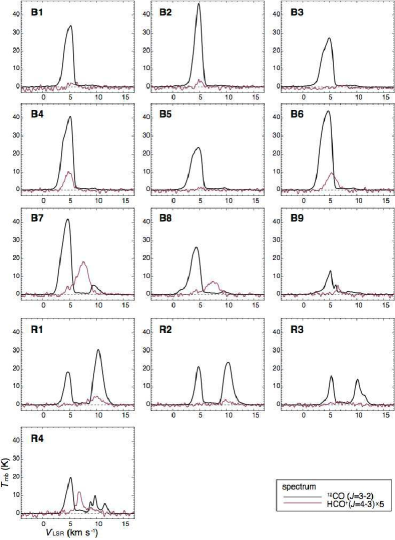
Figure 12: The ${\rm{}^{12}CO}$ ($J=3-2$) (black) and ${\rm HCO^{+}}$ ($J=4-3$) (red) spectra averaged over the surface areas of the identified outflow lobes. The ${\rm HCO^{+}}$ spectra are scaled up by a factor of 5.

where $V{\rm{}_{sys}}$ is the systemic velocity. In order to decide $V\rm_{sys}$, we derived the ${\rm HCO^{+}}$ spectra averaged over the surface areas of each outflow lobe. We then fitted the spectra with a single Gaussian function, and regarded the peak velocity of the Gaussian function as the systemic velocity $V\rm_{sys}$. In Figure 12, we show the ${\rm HCO^{+}}$ and ${\rm{}^{12}CO}$ spectra averaged over the surface areas of the identified high velocity lobes. The ${\rm HCO^{+}}$ emission line of B3 is not detected, for which we assumed $V{\rm{}_{sys}}=5$ km s${}^{-1}\,$for the lobe. Using Equations (C5)–(C7), we calculated $M_{\rm flow}$, $P_{\rm flow}$, and $E_{\rm flow}$ for the individual outflow lobe.

Next, we attempted to estimate the dynamical timescale, $t_{\rm d}$, of a outflow lobe. In general, $t_{\rm d}$ should be calculated using the maximum separation between the outflow lobes and the driving sources. For the outflow candidates found in W40, however, we cannot identify the definite driving sources and also cannot separate the individual outflow lobes reliably. We therefore estimated the dynamical timescale as $t_{\rm d}=R_{\rm flow}/V_{\rm char}$ where $R_{\rm flow}$ is the radius of the lobes defined as $R_{\rm flow}=\sqrt{S_{\rm lobe}/\pi}$ and $V_{\rm char}$ is the maximum difference between $V_{\rm sys}$ and the velocities observed in the high velocity wings detected at $>3\sigma$ ($\simeq 0.5$ K) noise level in the ${\rm{}^{12}CO}$ spectra observed at the intensity peak positions of the outflow lobes. We summarize the physical parameters of the 13 lobes derived in this appendix in Table 2.

Table 1: Velocity Components Observed in W40

$V_{\rm LSR}$	Detection	Detection	Comment
(km s-1)	in HCO+	in CO
$\sim 3$	Yes	Yes	Faint CO and HCO+ emission which might be unrelated to W40.
$\sim 5$	Yes	Yes	Intense CO emission ($\gtrsim 40$ K) originating from
			the dense gas associated with the expanding shell of the H ii region.
$\sim 7$	Yes	Faint	Systemic velocity component of the entire W40 region
		($\sim 2$ K)	causing heavy absorption in the CO emission line.
$\sim 10$	Yes	Yes	Intense CO emission ($\gtrsim 40$ K) originating from
			the dense gas associated with the expanding shell of the H ii region.

Table 2: Properties of the Candidates of Outflows

	Peak Position
Lobe	$\alpha$(J2000)	$\delta$(J2000)	$S_{\rm lobe}$	$\int\int T_{\rm mb}\,dvdS$	$V_{\rm sys}$	$V_{\rm char}$	$M_{\rm flow}$	$P_{\rm flow}$	$E_{\rm flow}$	$R_{\rm flow}$	$t_{\rm d}$
	($\rm{}^{h}\>{}^{m}\>{}^{s}$)	(${\arcdeg}\>{\arcmin}\>\>{\arcsec}$)	(arcmin2)	(K km s-1arcmin2)	(km s-1)	(km s-1)	($M_{\sun}$)	($M_{\sun}$ km s-1)	($M_{\sun}$ km2 s-2)	(pc)	(104yr)
B1	18 31 11.0	$-2$ 02 45	0.5	1.0	5.7	5.5	0.002	0.01	0.02	0.06	1.0
B2	18 31 11.7	$-2$ 03 45	1.2	3.8	5.0	6.7	0.007	0.03	0.07	0.09	1.3
B3	18 31 19.0	$-2$ 03 05	2.6	12.6	5.0	9.3	0.023	0.08	0.19	0.13	1.4
B4	18 31 11.0	$-2$ 06 45	1.5	4.2	4.8	5.5	0.008	0.03	0.05	0.10	1.8
B5	18 31 11.7	$-2$ 08 15	1.8	7.5	5.2	5.3	0.014	0.05	0.09	0.11	2.0
B6	18 31 15.7	$-2$ 07 25	1.8	9.9	5.4	5.0	0.018	0.06	0.11	0.11	2.2
B7	18 31 19.7	$-2$ 06 45	1.6	5.8	7.4	6.4	0.011	0.06	0.18	0.11	1.6
B8	18 31 22.3	$-2$ 07 25	2.0	14.3	7.3	8.3	0.026	0.14	0.41	0.12	1.4
B9	18 31 53.7	$-2$ 02 25	0.7	1.2	6.6	6.1	0.002	0.01	0.03	0.07	1.1
R1	18 31 26.3	$-2$ 05 25	1.5	4.9	9.8	4.2	0.009	0.02	0.03	0.10	2.3
R2	18 31 31.7	$-2$ 05 25	1.3	3.8	10.1	4.3	0.007	0.02	0.02	0.10	2.1
R3	18 31 40.3	$-2$ 02 05	0.5	0.8	7.1	6.3	0.002	0.01	0.02	0.06	0.9
R4	18 31 48.3	$-2$ 02 05	0.3	0.5	6.8	6.6	0.001	0.01	0.01	0.05	0.7

Note. — The velocity range $V_{\rm wing}$ used in Equations (C4)–(C7) to calculate $\int T_{\rm mb}dv$ is set to $-3.2\leqq V_{\rm LSR}\leqq 2.8$ km s^-1 for the blue lobes (B1–B9), and $11.7\leqq V_{\rm LSR}\leqq 14.5$ km s^-1 for the red lobes (R1–R4).

Table 3: Molecular Constants

Molecule	Transition	$S_{ij}$	$B_{0}$	$\mu$	$E_{u}$
			(GHz)	(Debye)	(cm-1)
${\rm{}^{12}CO}$	$J=3-2$	3.0	57.6350	0.110	23.0690
${\rm HCO^{+}}$	$J=4-3$	4.0	44.5944	3.888	29.7490

Note. — All of the constants are taken from JPL Catalog and Splatalogue.

Table 4: Properties of the Clumps

	Peak Position
clump	$\alpha$(J2000)	$\delta$(J2000)	$T_{\rm mb}$	$V_{\rm LSR}$	$\Delta V$	${N}$(HCO${}^{+})$	$S_{\rm clump}$	$\int\int T_{\rm mb}\,{\rm d}v{\rm d}S$	$M_{\rm clump}$	Associated
	($\rm{}^{h}\>{}^{m}\>{}^{s}$)	(${\arcdeg}\>{\arcmin}\>\>{\arcsec}$)	(K)	(km s-1)	(km s-1)	(cm-2)	(arcmin2)	(K km s-1arcmin2)	($M_{\sun}$)	Outflow Lobes
1	18 31 19.0	$-2$ 07 05	3.5	5.7	3.2	5.5$\times 10^{12}$	8.4	19.3	14.3	B1,B2,B4,B5,B6
										(B3)
2	18 31 21.0	$-2$ 06 25	8.1	7.6	2.3	1.1$\times 10^{13}$	5.3	24.0	17.8	B7,B8
3	18 31 33.7	$-2$ 04 15	4.5	8.0	1.7	3.8$\times 10^{12}$	3.4	10.2	7.6	(R3)
4	18 31 46.3	$-2$ 04 25	6.4	6.9	1.5	5.1$\times 10^{12}$	14.4	35.4	26.2	B9,R4
										(R3)
5	18 31 26.3	$-2$ 05 45	1.6	10.3	2.3	1.7$\times 10^{12}$	2.8	4.6	3.4	R1,R2
6	18 31 36.3	$-2$ 03 55	3.4	9.1	1.7	2.9$\times 10^{12}$	1.5	2.7	2.0	$\cdots$

Note. — The mass of Clump No. 6 may be underestimated by $\sim 50\%$, because of the fixed velocity range used to define the clumps ($9\leqq V_{\rm LSR}\leqq 12$ km s^-1). The other half of the mass is included in the Clump 3. The outflow lobe B3 is outside of the surface area of Clump 1, but we regarded them to be associated with each other, because they are close to each other on the sky. Another outflow lobe R3 is located right in the middle of Clumps 3 and 4, and we cannot judge which clump R3 is associated with.

Figure 6: (a) Locations of blue lobes of the outflow candidates which are labeled “B1”–“B9”. White plus signs denote the peak positions of the lobes. Blue solid and red broken contours represent the ${\rm{}^{12}CO}$ intensity integrated over the velocity range $-3.2\leqq V_{\rm LSR}\leqq 2.8$ km s${}^{-1}\,$and $5.7\leqq V_{\rm LSR}\leqq 8.4$ km s${}^{-1}\,$, respectively. The former contours are to search for the blue lobes of outflows, and the latter contours are made for a reference (see text and Figure 5). The lowest contour and the contour interval are 1.2 K km s${}^{-1}\,$, and symbols for the YSOs are the same as in Figure 1. Clumps indicated by thin solid circles with arrows are due to the distinct velocity component (at $\sim 3$ km s${}^{-1}\,$) unrelated to the lobes of the outflow candidates. (b) Same as (a), but for red lobes of the outflow candidates. Identified lobes are labeled “R1”–“R4”. Red solid and blue broken contours represent the ${\rm{}^{12}CO}$ intensity integrated over the velocity range $11.7\leqq V_{\rm LSR}\leqq 14.5$ km s${}^{-1}\,$and $8.5\leqq V_{\rm LSR}\leqq 9.2$ km s${}^{-1}\,$, respectively. The former contours are to search for the red lobes of outflows, and the latter contours are made for a reference (see text and Figure 5).

Figure 8: Top panel shows the total integrated intensity map of HCO⁺ same as Figure 1(b) overlaid with the candidate outflow lobes. The other three panels below the top panel display the channel maps for the $\sim 5$ km s${}^{-1}\,$, $\sim 7$ km s${}^{-1}\,$, and $\sim 10$ km s${}^{-1}\,$components integrated over the range $3\leqq V_{\rm LSR}\leqq 6$ km s${}^{-1}\,$, $6\leqq V_{\rm LSR}\leqq 9$ km s${}^{-1}\,$, and $9\leqq V_{\rm LSR}\leqq 12$ km s${}^{-1}\,$, respectively. Six identified clumps are indicated in these panels. The lowest contours and the contour intervals in the three panels are 1 K km s^-1. Peak positions of the six clumps are indicated by red plus signs. The symbols for the YSOs are the same as in Figure 1. The ${\rm HCO^{+}}$ spectra sampled at the peak positions are also shown.

References

- André et al. (2010) André, P., Men’shchikov, A., Bontemps, S., et al. 2010, A&A, 518, L102
- Arce et al. (2010) Arce, H. G., Borkin, M. A., Goodman, A. A., Pineda, J. E., & Halle, M. W. 2010, ApJ, 715, 1170
- Bally et al. (1999) Bally, J., Reipurth, B., Lada, C. J., & Billawala, Y. 1999, AJ, 117, 410
- Bontemps et al. (2010) Bontemps, S., André, P., Könyves, V., et al. 2010, A&A, 518, L85
- Bradshaw et al. (2015) Bradshaw, C., Offner, S. S. R., & Arce, H. G. 2015, ApJ, 802, 86
- Crutcher (1977) Crutcher, R. M. 1977, ApJ, 216, 308
- Dobashi (2011) Dobashi, K. 2011, PASJ, 63, 1
- Dobashi et al. (1998) Dobashi, K., Sato, F., & Mizuno, A. 1998, PASJ, 50, L15
- Dobashi et al. (2005) Dobashi, K., Uehara, H., Kandori, R., et al. 2005, PASJ, 57, 1
- Dunham et al. (2014) Dunham, M. M., Arce, H. G., Mardones, D., et al. 2014, ApJ, 783, 29
- Dzib et al. (2010) Dzib, S., Loinard, L., Mioduszewski, A. J., et al. 2010, ApJ, 718, 610
- Elmegreen & Lada (1977) Elmegreen, B. G., & Lada, C. J. 1977, ApJ, 214, 725
- Ezawa et al. (2004) Ezawa, H., Kawabe, R., Kohno, K., & Yamamoto, S. 2004, in Society of Photo-Optical Instrumentation Engineers (SPIE) Conference Series, Vol. 5489, Ground-based Telescopes, ed. J. M. Oschmann, Jr., 763–772
- Frerking et al. (1982) Frerking, M. A., Langer, W. D., & Wilson, R. W. 1982, ApJ, 262, 590
- Girart et al. (2000) Girart, J. M., Estalella, R., Ho, P. T. P., & Rudolph, A. L. 2000, ApJ, 539, 763
- Hirahara et al. (1992) Hirahara, Y., Suzuki, H., Yamamoto, S., et al. 1992, ApJ, 394, 539
- Hirano et al. (2006) Hirano, N., Liu, S.-Y., Shang, H., et al. 2006, ApJ, 636, L141
- Hirota et al. (2009) Hirota, T., Ohishi, M., & Yamamoto, S. 2009, ApJ, 699, 585
- Kirsanova et al. (2014) Kirsanova, M. S., Wiebe, D. S., Sobolev, A. M., Henkel, C., & Tsivilev, A. P. 2014, MNRAS, 437, 1593
- Kohno et al. (2004) Kohno, K., Yamamoto, S., Kawabe, R., et al. 2004, in The Dense Interstellar Medium in Galaxies, ed. S. Pfalzner, C. Kramer, C. Staubmeier, & A. Heithausen, 349
- Könyves et al. (2010) Könyves, V., André, P., Men’shchikov, A., et al. 2010, A&A, 518, L106
- Kuhn et al. (2010) Kuhn, M. A., Getman, K. V., Feigelson, E. D., et al. 2010, ApJ, 725, 2485
- Kutner & Ulich (1981) Kutner, M. L., & Ulich, B. L. 1981, ApJ, 250, 341
- Mallick et al. (2013) Mallick, K. K., Kumar, M. S. N., Ojha, D. K., et al. 2013, ApJ, 779, 113
- Maury et al. (2011) Maury, A. J., André, P., Men’shchikov, A., Könyves, V., & Bontemps, S. 2011, A&A, 535, A77
- Mikami et al. (1992) Mikami, H., Umemoto, T., Yamamoto, S., & Saito, S. 1992, ApJ, 392, L87
- Nakamura & Li (2007) Nakamura, F., & Li, Z.-Y. 2007, ApJ, 662, 395
- Nakamura et al. (2011) Nakamura, F., Sugitani, K., Shimajiri, Y., et al. 2011, ApJ, 737, 56
- Nakamura et al. (2014) Nakamura, F., Sugitani, K., Tanaka, T., et al. 2014, ApJ, 791, L23
- Offner et al. (2011) Offner, S. S. R., Lee, E. J., Goodman, A. A., & Arce, H. 2011, ApJ, 743, 91
- Pirogov et al. (2013) Pirogov, L., Ojha, D. K., Thomasson, M., Wu, Y.-F., & Zinchenko, I. 2013, MNRAS, 436, 3186
- Rodney & Reipurth (2008) Rodney, S. A., & Reipurth, B. 2008, The W40 Cloud Complex, ed. B. Reipurth, 683
- Rodríguez et al. (2010) Rodríguez, L. F., Rodney, S. A., & Reipurth, B. 2010, AJ, 140, 968
- Sawada et al. (2008) Sawada, T., Ikeda, N., Sunada, K., et al. 2008, PASJ, 60, 445
- Schwab (1984) Schwab, F. R. 1984, in Indirect Imaging. Measurement and Processing for Indirect Imaging, ed. J. A. Roberts, 333–346
- Shimajiri et al. (2008) Shimajiri, Y., Takahashi, S., Takakuwa, S., Saito, M., & Kawabe, R. 2008, ApJ, 683, 255
- Shimajiri et al. (2009) —. 2009, PASJ, 61, 1055
- Shimoikura & Dobashi (2011) Shimoikura, T., & Dobashi, K. 2011, ApJ, 731, 23
- Shimoikura et al. (2012) Shimoikura, T., Dobashi, K., Sakurai, T., et al. 2012, ApJ, 745, 195
- Shimoikura et al. (2013) Shimoikura, T., Dobashi, K., Saito, H., et al. 2013, ApJ, 768, 72
- Shuping et al. (2012) Shuping, R. Y., Vacca, W. D., Kassis, M., & Yu, K. C. 2012, AJ, 144, 116
- Suzuki et al. (1992) Suzuki, H., Yamamoto, S., Ohishi, M., et al. 1992, ApJ, 392, 551
- Tokuda et al. (2013) Tokuda, K., Kozu, M., Kimura, K., et al. 2013, in Astronomical Society of the Pacific Conference Series, Vol. 476, Astronomical Society of the Pacific Conference Series, ed. R. Kawabe, N. Kuno, & S. Yamamoto, 403
- Vallee (1987) Vallee, J. P. 1987, A&A, 178, 237
- van der Tak et al. (2007) van der Tak, F. F. S., Black, J. H., Schöier, F. L., Jansen, D. J., & van Dishoeck, E. F. 2007, A&A, 468, 627
- Wang et al. (1994) Wang, Y., Jaffe, D. T., Graf, U. U., & Evans, II, N. J. 1994, ApJS, 95, 503
- Wu et al. (2004) Wu, Y., Wei, Y., Zhao, M., et al. 2004, A&A, 426, 503
- Zeilik & Lada (1978) Zeilik, II, M., & Lada, C. J. 1978, ApJ, 222, 896
- Zhu et al. (2006) Zhu, L., Wu, Y.-F., & Wei, Y. 2006, Chinese J. Astron. Astrophys., 6, 61