Solutions to Integrals Involving the Marcum $Q-$Function and Applications

Abstract

Novel analytic solutions are derived for integrals that involve the generalized Marcum $Q-$function, exponential functions and arbitrary powers. Simple closed-form expressions are also derived for specific cases of the generic integrals. The offered expressions are both convenient and versatile, which is particularly useful in applications relating to natural sciences and engineering, including wireless communications and signal processing. To this end, they are employed in the derivation of the average probability of detection in energy detection of unknown signals over multipath fading channels as well as of the channel capacity with fixed rate and channel inversion in the case of correlated multipath fading and switched diversity.

I Introduction

The generalized Marcum $Q{-}$function, $Q_{m}(a,b)$, has been extensively involved in numerous areas of wireless communications including digital communications over fading channels, information-theoretic analysis of multi-antenna systems, cognitive radio communications, radar systems, [1, 2, 3, 4, 5, 6, 7, 8] and references therein. Furthermore, its use has enabled the derivation of several tractable analytic expressions for important performance measures in communication theory [4].

The derivation of tractable analytic expressions in natural sciences and engineering is typically a tedious, if not impossible, task because cumbersome integrals are often encountered [9, 13, 16, 21, 20, 10, 11, 12, 14, 15, 17, 18, 19, 22]. This is also the case when the Marcum $Q{-}$function is involved in integrands along with exponential functions and arbitrary power terms. Two such integrals are the following:

$$\mathcal{G}(k,m,a,b,p)=\int_{0}^{\infty}x^{k-1}Q_{m}(a,b\sqrt{x})e^{-px}{\rm d}x$$ (1)

and

$$\mathcal{F}(k,m,a,b,p)=\int_{0}^{\infty}x^{k-1}Q_{m}(a\sqrt{x},b)e^{-px}{\rm d}x.$$ (2)

These integrals have been widely employed in the analysis of multi-channel receivers with non-coherent and differentially coherent detection as well as in the detection of unknown signals in cognitive radio and radar systems [9, 23, 24, 25, 28, 35, 38, 37, 36, 34, 30, 31, 32, 26, 27, 29, 33] and the references therein. Based on this, a recursive formula for (2), that is restricted to only integer values of $k$ and $m$, was firstly reported in [2]. Likewise, exact infinite series for (1) and (2) were proposed in [16] while a closed-form solution to (2) for integer values of $k$ was recently reported in [21].

Nevertheless, the existing expressions for (1) and (2) are subject to validity restrictions, which limit the generality of the involved parameters and often render them inconvenient to use in applications of interest. Motivated by this, the present work is devoted to the derivation of novel closed-form expressions for (1) and (2), which are more generic and have a relatively tractable algebraic representation. These characteristics render them useful in several analyses in natural sciences and engineering, including the broad areas of wireless communications and signal processing. To this end, they are subsequently employed in the derivation of closed-form expressions for the following indicative applications: $i)$ the average probability of detection in energy detection over Nakagami$-m$ multipath fading channels which, unlike previous analyses, is valid for arbitrary values of $m$; $ii)$ the channel capacity with channel inversion and fixed rate in arbitrarily correlated Nakagami$-m$ fading conditions using switch-and-stay combining. The derived expressions are validated extensively through comparisons with respective computer simulations results.

II Analytic Solutions to Integrals Involving Power, Exponential and Marcum $Q-$functions

II-A Closed-form Solutions to $\mathcal{G}(k,m,a,b,p)$

Theorem 1.

For $a,b\in\mathbb{R}$, $m\in\mathbb{N}$ and $k,p\in\mathbb{R^{+}}$, the following closed-form representation holds

$$\mathcal{G}(k,m,a,b,p)=\frac{\Gamma(k)}{p^{k}}-\left(\frac{2}{b^{2}+2p}\right)^{k}e^{-\frac{a^{2}}{2}}\Gamma(k)\qquad\qquad\qquad\qquad\qquad\qquad\qquad\qquad\qquad\qquad\qquad\qquad$$ (3)

$$\times\left[\Phi_{1}\left(k,1,1;\frac{b^{2}}{b^{2}+2p},\frac{a^{2}b^{2}}{2b^{2}+4p}\right)-\sum_{n=0}^{m-1}\frac{(k)_{n}}{n!}\left(\frac{b^{2}}{b^{2}+2p}\right)^{n}\,_{1}F_{1}\left(k+n;n+1;\frac{a^{2}b^{2}}{2b^{2}+4p}\right)\right]$$

where $\Gamma(\cdot)$, $\Phi_{1}(\cdot)$ and ${}_{1}F_{1}(\cdot)$ denote the Euler Gamma function, the Humbert hypergeometric function of the first kind and the Kummer hypergeometric function, respectively [39].

Proof.

The series in [16, eq. (10)] can be re-written as follows

$$\begin{split}\mathcal{G}(k,m,a,b,p)=&\sum_{n=0}^{m-1}\frac{\Gamma(k+n)\,_{1}F_{1}\left(k+n;n+1;\frac{a^{2}b^{2}}{2b^{2}+4p}\right)}{n!b^{-2n}2^{-k}(b^{2}+2p)^{k+n}e^{\frac{a^{2}}{2}}}+\frac{\Gamma(k)}{p^{k}}\\ &-\underbrace{\frac{2^{k}}{e^{\frac{a^{2}}{2}}}\sum_{n=0}^{\infty}\frac{\Gamma(k+n)b^{2n}\,_{1}F_{1}\left(k+n;n+1;\frac{a^{2}b^{2}}{2b^{2}+4p}\right)}{n!(b^{2}+2p)^{k+n}}}_{\mathcal{A}(k,a,b,p)}.\end{split}$$ (4)

Using the infinite series in [40, eq. (9.14.1)], it follows that

$$\mathcal{A}(k,a,b,p)=\sum_{n=0}^{\infty}\sum_{l=0}^{\infty}\frac{a^{2l}b^{2n+2l}\Gamma(n+k)e^{-\frac{a^{2}}{2}}(k+n)_{l}}{n!l!2^{l-k}(b^{2}+2p)^{n+k+l}(1+n)_{l}}$$ (5)

where $(x)_{n}$ denotes the Pochhammer symbol. Given that

$$(k+n)_{l}=\frac{(k)_{n+l}}{(k)_{n}}$$ (6)

and

$$(1+n)_{l}=\frac{(1)_{n+l}}{(1)_{n}}$$ (7)

one obtains

$$\mathcal{A}(k,a,b,p)=\mathcal{B}\sum_{n=0}^{\infty}\sum_{l=0}^{\infty}\frac{(k)_{n+l}(1)_{n}}{(1)_{n+l}}\frac{\left(\frac{b^{2}}{b^{2}+2p}\right)^{n}}{n!}\frac{\left(\frac{a^{2}b^{2}}{2b^{2}+4p}\right)^{l}}{l!}$$ (8)

where

$$\mathcal{B}=\frac{2^{k}\Gamma(k)\exp(a^{2}/2)}{(b^{2}+2p)^{k}}$$ (9)

Notably, eq. (8) can be expressed in terms of the Humbert function, $\Phi_{1}$, namely

$$\mathcal{A}(k,a,b,p)=\frac{2^{k}\,\Gamma(k)\,e^{-\frac{a^{2}}{2}}}{(b^{2}+2p)^{k}\,}\Phi_{1}\left(k,1,1;\frac{b^{2}}{b^{2}+2p},\frac{a^{2}b^{2}}{2b^{2}+4p}\right)$$ (10)

Inserting (10) in (4) yields (3), which completes the proof. ∎

It is noted that Humbert functions and their properties have been studied extensively over the past decades [40, 39].

Theorem 2.

For $a,b\in\mathbb{R}$ and $m,p\in\mathbb{R}^{+}$ and $k\in\mathbb{N}$, the following closed-form expression holds

$$\mathcal{G}(k,m,a,b,p)=\frac{\Gamma(k)}{p^{k}}-\frac{\Gamma(k)\,b^{2m}e^{-\frac{a^{2}}{2}}}{p^{k}(b^{2}+2p)^{m}}\sum_{l=0}^{k-1}\frac{(m)_{l}(2p)^{l}}{l!(b^{2}+2p)^{l}}\,_{1}F_{1}\left(l+m;m;\frac{a^{2}b^{2}}{2b^{2}+4p}\right).$$ (11)

Proof.

By integrating (1) by parts, it follows that

$$\mathcal{G}(k,m,a,b,p)=\lim_{x\to\infty}\,g(x)\int\frac{x^{k}\,{\rm d}x}{x\,e^{px}}-\lim_{x\to 0}\,g(x)\int\frac{x^{k}\,{\rm d}x}{x\,e^{px}}-\int_{0}^{\infty}\left[\int\frac{x^{k-1}}{e^{px}}{\rm d}x\right]\,\frac{{\rm d}}{{\rm d}x}Q_{m}(a,b\sqrt{x}){\rm d}x$$ (12)

where

$$g(x)=Q_{m}(a,b\sqrt{x})$$ (13)

The integrals in (12) can be expressed in terms of the incomplete gamma function yielding

$$\mathcal{G}(k,m,a,b,p)=\lim_{x\to\infty}\,g(x)\frac{\Gamma(k,px)}{p^{k}}-\lim_{x\to 0}\,g(x)\frac{\Gamma(k,px)}{p^{k}}-\frac{1}{p^{k}}\int_{0}^{\infty}\Gamma(k,px)\,\frac{{\rm d}}{{\rm d}x}Q_{m}(a,b\sqrt{x}){\rm d}x.$$ (14)

Recalling the identities

$$\Gamma(a,\infty)=0,$$ (15)

$$\Gamma(a,0)=\Gamma(a)$$ (16)

and

$$Q_{m}(a,0)=1$$ (17)

as well as setting $u=\sqrt{x}$ in (14) along with utilizing [2, eq. (9)] and [40, eq. (8.352.4)], it follows that

$$\mathcal{G}(k,m,a,b,p)=\frac{\Gamma(k)}{p^{k}}\times\left[1-a^{1-m}e^{-\frac{a^{2}}{2}}\sum_{l=0}^{k-1}\frac{p^{l}}{l!b^{2l}}\int_{0}^{\infty}x^{m-2l}e^{-\left(\frac{p}{b^{2}}+\frac{1}{2}\right)x^{2}}I_{m-1}(ax)\,{\rm d}x\right].$$ (18)

The above integral can be expressed in closed-form using [40, eq. (6.621.1)]. To this effect, eq. (18) is deduced, which completes the proof. ∎

II-B Closed-form Solutions to $\mathcal{F}(k,m,a,b,p)$

A closed-form expression for (2) was reported in [21] for the case that $k$ is integer and $m$ is arbitrary real, namely

$$\begin{split}\mathcal{F}(k,m,a,b,p)=&\frac{\Gamma(k)\Gamma\left(m,\frac{b^{2}}{2}\right)}{p^{k}\Gamma(m)}\\ &+\frac{a^{2}b^{2m}\Gamma(k)e^{-\frac{b^{2}}{2}}}{m!p^{k}2^{m}(a^{2}+2p)}\sum_{l=0}^{k-1}\left(\frac{2p}{a^{2}+2p}\right)^{l}\,_{1}F_{1}\left(l+1;m+1;\frac{a^{2}b^{2}}{2a^{2}+4p}\right).\end{split}$$ (19)

Likewise, in what follows we derive a closed-form expression for the useful case that $m$ is integer and $k$ is arbitrary real.

Theorem 3.

For $k,p\in\mathbb{R^{+}}$, $m\in\mathbb{N}$ and $a,b\in\mathbb{R}$, the following closed-form expression is valid

$$\mathcal{F}(k,m,a,b,p)=\frac{\Gamma(k)}{p^{k}}-\frac{2^{k}\Gamma(k)e^{-\frac{b^{2}}{2}}\Phi_{2}\left(1,k,1;\frac{b^{2}}{2},\frac{a^{2}b^{2}}{2a^{2}+4p}\right)}{(a^{2}+2p)^{k}}\qquad\qquad\qquad$$ (20)

$$\qquad\quad+\frac{\Gamma(k)2^{k}e^{-\frac{b^{2}}{2}}}{(a^{2}+2p)^{k}}\sum_{n=0}^{m-1}\frac{b^{2n}}{n!2^{n}}\,_{1}F_{1}\left(k;n+1;\frac{a^{2}b^{2}}{2a^{2}+4p}\right)$$

where $\Phi_{2}(\cdot)$ is the Humbert function of the second kind [40].

Proof.

The series in [16, eq. (9)] can be also expressed as

$$\begin{split}\mathcal{F}(k,m,a,b,p)=&\frac{\Gamma(k)}{p^{k}}+\sum_{n=0}^{m-1}\frac{\Gamma(k)_{1}F_{1}\left(k;n+1;\frac{a^{2}b^{2}}{2a^{2}+4p}\right)}{n!b^{-2n}2^{n-k}(a^{2}+2p)^{k}e^{\frac{b^{2}}{2}}}\\ &-\underbrace{\frac{\Gamma(k)2^{k}e^{-\frac{b^{2}}{2}}}{(a^{2}+2p)^{k}}\sum_{n=0}^{\infty}\frac{b^{2n}}{n!2^{n}}\,_{1}F_{1}\left(k;n+1;\frac{a^{2}b^{2}}{2a^{2}+4p}\right)}_{\mathcal{H}(k,a,b,p)}.\end{split}$$ (21)

Applying [40, eq. (9.14.1)] in $\mathcal{H}(k,a,b,p)$ and given that

$$(n+1)_{l}=\frac{\Gamma(n+l+1)}{\Gamma(n+1)}=\frac{(1)_{n+l}}{(1)_{n}}$$ (22)

one obtains

$$\mathcal{H}(k,a,b,p)=\frac{e^{-\frac{b^{2}}{2}}2^{k}\Gamma(k)}{(a^{2}+2p)^{k}}\sum_{n=0}^{\infty}\sum_{l=0}^{\infty}\frac{(1)_{n}(k)_{l}}{(1)_{n+l}}\frac{\frac{b^{2n}}{2^{n}}}{n!}\frac{\left(\frac{a^{2}b^{2}}{2a^{2}+4p}\right)^{l}}{l!}.$$ (23)

Notably, the above expression can be expressed in terms of the Humbert hypergeometric function of the second kind yielding

$$\mathcal{H}(k,a,b,p)=\frac{e^{-\frac{b^{2}}{2}}2^{k}\Gamma(k)}{(a^{2}+2p)^{k}}\Phi_{2}\left(1,k,1;\frac{b^{2}}{2},\frac{a^{2}b^{2}}{2a^{2}+4p}\right).$$ (24)

Inserting (24) into (21) yields (20), concluding the proof. ∎

II-C Specific Cases of $\mathcal{F}(k,m,a,b,p)$ and $\mathcal{G}(k,m,a,b,p)$

Simple expressions are derived for $k=1$, $a=0$ and $b=0$.

II-C1 The case that $k=1$

In this special case it follows that

$$\mathcal{G}(1,m,a,b,p)=\int_{0}^{\infty}Q_{m}(a,b\sqrt{x})e^{-px}{\rm d}x$$ (25)

and

$$\mathcal{F}(1,m,a,b,p)=\int_{0}^{\infty}Q_{m}(a\sqrt{x},b)e^{-px}{\rm d}x.$$ (26)

Equation (25) is given by [16, eq. (16)]. In the same context, a generic closed-form expression for (26) is derived below.

Lemma 1.

For $a,m\in\mathbb{R}$ and $b,p\in\mathbb{R}^{+}$, the following closed-form expression is valid

$$\mathcal{F}(1,m,a,b,p)=\frac{\Gamma\left(m,\frac{b^{2}}{2}\right)}{p\Gamma(m)}+\frac{a^{2}e^{-\frac{pb^{2}}{a^{2}+2p}}\gamma\left(m,\frac{a^{2}b^{2}}{2a^{2}+4p}\right)}{pa^{2m}\Gamma(m)(a^{2}+2p)^{1-m}}$$ (27)

where $\gamma(a,x)$ denotes the lower incomplete gamma function.

Proof.

By setting $k=1$ in (19), it immediately follows that

$$\mathcal{F}(1,m,a,b,p)=\frac{\Gamma\left(m,\frac{b^{2}}{2}\right)}{p\Gamma(m)}+\frac{a^{2}b^{2m}\,_{1}F_{1}\left(1;m+1;\frac{a^{2}b^{2}}{2a^{2}+4p}\right)}{m!p2^{m}(a^{2}+2p)e^{\frac{b^{2}}{2}}}$$ (28)

Notably, using the following hypergeometric function identity

$$\,{}_{1}F_{1}(1;n;x)=x^{1-n}(n-1)e^{x}\gamma(n-1,x)$$ (29)

and recalling that

$$\gamma(a,x)=\Gamma(a)-\Gamma(a,x)$$ (30)

and

$$\frac{m!}{m}=(m-1)!=\Gamma(m)$$ (31)

equation (28) can be equivalently expressed as

$$\mathcal{F}(1,m,a,b,p)=\frac{\Gamma\left(m,\frac{b^{2}}{2}\right)}{p\,\Gamma(m)}+\frac{(a^{2}+2p)^{m-1}e^{-\frac{a^{2}b^{2}}{a^{2}+2p}}}{p\,a^{2m-2}}-\frac{(a^{2}+2p)^{m-1}e^{-\frac{a^{2}b^{2}}{a^{2}+2p}}}{p\,a^{2m-2}\Gamma(m)}\Gamma\left(m,\frac{a^{2}b^{2}}{2a^{2}+4p}\right).$$ (32)

To this effect and performing long but basic algebraic manipulations (32) reduces to (27), which completes the proof. ∎

Remark 1.

A similar expression can be obtained through (20).

II-C2 The case that $a=0$

In this special case it follows that

$$\mathcal{G}(k,m,0,b,p)=\int_{0}^{\infty}x^{k-1}Q_{m}(0,b\sqrt{x})e^{-px}{\rm d}x$$ (33)

and

$$\mathcal{F}(k,m,0,b,p)=Q_{m}(0,b)\int_{0}^{\infty}x^{k-1}e^{-px}{\rm d}x.$$ (34)

Lemma 2.

For $k,p\in\mathbb{R}^{+}$, $m\in\mathbb{N}$ and $b\in\mathbb{R}$, the following closed-form representations hold

$$\mathcal{G}(k,m,0,b,p)=\frac{2^{k}}{(b^{2}+2p)^{k}}\sum_{l=0}^{m-1}\frac{b^{2l}\Gamma(k+l)}{l!(b^{2}+2p)^{l}}$$ (35)

and

$$\mathcal{F}(k,m,0,b,p)=\frac{\Gamma(k)}{p^{k}}e^{-\frac{b^{2}}{2}}\sum_{l=0}^{m-1}\frac{b^{2l}}{l!2^{l}}.$$ (36)

Proof.

Applying [2, eq. (2)] in (33) one obtains

$$\mathcal{G}(k,m,0,b,p)=\sum_{l=0}^{m-1}\frac{b^{2l}}{l!2^{l}}\int_{0}^{\infty}x^{k+l-1}e^{-x\left(p+\frac{b^{2}}{2}\right)}{\rm d}x.$$ (37)

Evidently, the above integral can be expressed in closed-form in terms of the Euler gamma function. This is also the case for $\mathcal{F}(k,m,0,b,p)$ since $Q_{m}(0,b)$ is not a part of the integrand. As a result, by performing a necessary change of variables in [40, eq. (8.310.1)] and substituting (37) and (33) one obtains (35) and (34), respectively, which completes the proof. ∎

II-C3 The case that $b=0$

In this special case it follows that

$$\mathcal{G}(k,m,a,0,p)=Q_{m}(a,0)\int_{0}^{\infty}x^{k-1}e^{-px}{\rm d}x$$ (38)

and

$$\mathcal{F}(k,m,a,0,p)=\int_{0}^{\infty}x^{k-1}Q_{m}(a\sqrt{x},0)e^{-px}{\rm d}x.$$ (39)

Lemma 3.

For $p\in\mathbb{R}^{+}$ and $a,m,k\in\mathbb{R}$, the following simple closed-form expression is valid

$$\mathcal{G}(k,m,a,0,p)=\mathcal{F}(k,m,a,0,p)=\frac{\Gamma(k)}{p^{k}}.$$ (40)

Proof.

The proof follows with the aid of the identity $Q_{m}(a,0)\triangleq 1$, in [2, eq. (1)] as well as [40, eq. (8.310.1)]. ∎

III Applications in Wireless Communications

As already mentioned, the derived expressions for (1) and (2) can be used in applications relating to natural sciences and engineering, including wireless communications and signal processing. Based on this, they are employed in the derivation of simple expressions for the detection of unknown signals in cognitive radio and radar systems as well as for the channel capacity using switched diversity. To this end, a closed-form expression is firstly derived for the average probability of detection over Nakagami$-m$ fading channels. Likewise, a closed-form expression is derived for the channel capacity with channel inversion and fixed rate in switch-and-stay combining (SSC) under correlated Nakagami$-m$ fading conditions.

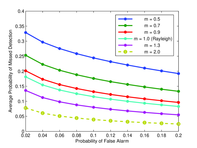
Figure 1: ROC curve for $u=5$, $\overline{\gamma}=15$dB and different values of $m$.

III-A Energy detection over Nakagami$-m$ fading channels with arbitrary values of $m$

The detection of unknown signals is modeled as a binary hypothesis-testing problem, where $H_{0}$ and $H_{1}$ denote the cases that a signal is absent or present, respectively. The corresponding test statistic is typically represented by the central chi-square and the non-central chi-square distributions, respectively, and is compared with an energy threshold, $\lambda$ [9].

Corollary 1.

For $\overline{\gamma},\lambda\in\mathbb{R}^{+}$, and either $m\geq 0.5$ and $u\in\mathbb{N}$, or $m\in\mathbb{N}$ and $u\in\mathbb{R}^{+}$, the average probability of detection over Nakagami$-m$ fading channels can be expressed as

$$\overline{P}_{d}=\frac{m^{m}}{\overline{\gamma}^{m}\Gamma(m)}\mathcal{F}\left(m,u,\sqrt{2},\sqrt{\lambda},\frac{m}{\overline{\gamma}}\right).$$ (41)

Proof.

The probability of false alarm and probability of detection in additive white Gaussian noise are given by $P_{f}=\Gamma(u,\lambda{/}2)$ and $P_{d}=Q_{u}(\sqrt{2\gamma},\sqrt{\lambda})$, respectively, where $u$ and $\gamma$ denote the time-bandwidth product and the instantaneous signal-to-noise ratio (SNR), respectively [21, 20, 23]. It is recalled that in energy detection over fading channels, the $P_{d}$ is averaged over the fading statistics. To this effect, for the case Nakagami$-m$ fading channels in [4, eq. (2. 21)] is represented as follows

$$\overline{P}_{d}=\frac{m^{m}}{\overline{\gamma}^{m}\Gamma(m)}\int_{0}^{\infty}\gamma^{m-1}Q_{u}(\sqrt{2\gamma},\sqrt{\lambda})e^{-\frac{m\gamma}{\overline{\gamma}}}{\rm d}\gamma.$$ (42)

Evidently, the above integral can be expressed in terms of (19) or (20). This yields (41), which completes the proof. ∎

Notably, the offered expression can account for arbitrary values of $m$, contrary to existing analyses that assume integer values of $m$ for simplicity. Fig. $1$ illustrates the corresponding probability of missed detection versus probability of false alarm ROC curve for different values of $m$. One can notice the sensitivity of $m$, particularly for small values, and thus, the usefulness of the offered expression also in practical scenarios.

III-B Capacity with channel inversion and fixed rate over correlated Nakagami$-m$ fading using switch-and-stay combining

Channel capacity under different transmission policies is particularly useful in achieving certain quality of service requirements. In this context, channel inversion with fixed rate (CIFR) has been rather useful as it ensures a constant SNR at the receiver through adaptation of the transmit power. This method relies on fixed-rate modulation and fixed code design, which renders its implementation relatively simple [4].

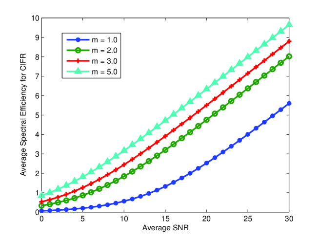
Figure 2: Average SE vs $\overline{\gamma}$ for CIFR under correlated Nakagami$-m$ fading with SSC for $\gamma_{T}=0$dB, $\rho=0.5$ and different values of $m$.

Corollary 2.

For $\overline{\gamma},B\in\mathbb{R}^{+}$, $m\geq\frac{1}{2}$ and $0\leq\rho<1$, the capacity with channel inversion and fixed rate over correlated Nakagami$-m$ fading channels with SSC can be expressed as

$$C_{\rm CIFR}=B\log_{2}\left(1+\frac{1}{\mathcal{R}(m,\overline{\gamma},\gamma_{T},\rho)}\right)$$ (43)

where

$$\mathcal{R}(m,\overline{\gamma},\gamma_{T},\rho)=\frac{m}{\overline{\gamma}\Gamma(m)}\Gamma\left(m-1,\frac{m\gamma_{T}}{\overline{\gamma}}\right)-\frac{m^{m}}{\overline{\gamma}^{m}\Gamma(m)}\mathcal{F}\left(m-1,m,\sqrt{\frac{2m\rho}{(1-\rho)\overline{\gamma}}},\sqrt{\frac{2m\gamma_{T}}{(1-\rho)\overline{\gamma}}},\frac{m}{\overline{\gamma}}\right)$$ (44)

with $\rho$ and $\gamma_{T}$ denoting the correlation coefficient and the predetermined SNR switching threshold, respectively.

Proof.

The CIFR over fading channels is defined as [41]

$$C_{\rm CIFR}=B\log_{2}\left(1+\frac{1}{\int_{0}^{\infty}\frac{p_{\gamma}(\gamma)}{\gamma}{\rm d}\gamma}\right).$$ (45)

In the case of switched diversity and correlated Nakagami$-m$ fading, the PDF of the SSC output is given by [4, eq. (9.334)]. By also setting

$$\mathcal{R}=\int_{0}^{\infty}\frac{p_{\gamma_{\rm SSC}}(\gamma)}{\gamma}\,{\rm d}\gamma$$ (46)

it follows that

$$\mathcal{R}=\int_{0}^{\infty}A(\gamma){\rm d}\gamma+\int_{\gamma_{T}}^{\infty}p_{\gamma}(\gamma){\rm d}\gamma$$ (47)

where $A(\gamma)$ is given in [4, eq. (9.335)]. To this effect and using [4, eq. (2. 21)] one obtains

$$\begin{split}\mathcal{R}(m,\overline{\gamma},\gamma_{T},\rho)=&\frac{m^{m}}{\overline{\gamma}^{m}\Gamma(m)}\int_{\gamma_{T}}^{\infty}\gamma^{m-2}e^{-\frac{m\gamma}{\overline{\gamma}}}\,{\rm d}\gamma\\ &-m^{m}\int_{0}^{\infty}\frac{\gamma^{m-2}\,e^{-\frac{m\gamma}{\overline{\gamma}}}}{\overline{\gamma}^{m}\Gamma(m)}Q_{m}\left(\sqrt{\frac{2m\rho\gamma}{(1-\rho)\overline{\gamma}}},\sqrt{\frac{2m\gamma_{T}}{(1-\rho)\overline{\gamma}}}\right){\rm d}\gamma.\end{split}$$ (48)

The first two integrals in (48) can be expressed in terms of the gamma functions, whereas the third integral has the algebraic form of (2). Therefore, by performing the necessary change of variables yields (43), which completes the proof. ∎

The behavior of the corresponding average spectral efficiency versus average SNR is illustrated in Fig. 2 for different values of $m$ with fixed values of $\gamma_{T}$ and $\rho$. The significant effect of the severity of fading on $C_{\rm CIFR}$ is clearly observed.

IV Conclusion

Novel closed-form expressions were derived for two Marcum $Q-$function integrals which are both simple and generic. Simple analytic expressions for involved special cases were also derived in closed-form. These expressions are tractable and are expected to be useful in analyses relating to natural sciences and engineering, including wireless communications and signal processing. To this end, they were employed in the analysis of energy detection in RADAR and cognitive radio systems as well as in the channel capacity with channel inversion and fixed rate over correlated multipath fading channels.

References

[1]
J. I. Marcum,
“Table of Q-functions, U.S. Air Force Project RAND Res. Memo. M-339, ASTIA document AD 1165451,”
RAND Corp., Santa Monica, CA, 1950.
[2] A. H. Nuttall,
Some integrals involving the function,
Naval underwater systems center, New London Lab, New London, CT, 1974.
[3]
M. K. Simon, and M.-S. Alouini,
“Some new results for integrals involving the generalized Marcum function and their application to performance evaluation over fading channels,”
IEEE Trans. Wireless Commun., vol. 2, no. 4, pp. 611615, July 2003.
[4]
M. K. Simon, and M.-S. Alouini,
Digital communication over fading channels,
Wiley, New York, 2005.
[5]
Yu. A. Brychkov,
“On some properties of the Marcum function,”
Integral Transforms and Special Functions, vol. 23, no. 3, pp. 177182, Mar. 2012.
[6]
T. Q. Duong, D. B. da Costa, M. Elkashlan, and V. N. Q. Bao,
“Cognitive amplify-and-forward relay networks over Nakagami fading,”
IEEE Trans. Veh. Technol., vol. 61, no. 5, pp. 23682374, May 2012.
[7]
P. J. Smith, P. A. Dmochowski, H. A. Suraweera, M. Shafi,
“The effects of limited channel knowledge on cognitive radio system capacity,”
IEEE Trans. Veh. Technol., vol. 62, no. 2, pp. 927933, Feb. 2013.
[8]
Z. Zhao, Z. Ding, M. Peng, W. Wang, and J. Thompson,
“On the design of cognitive radio inspired asymmetric network coding transmissions in MIMO systems,”
IEEE Trans. Veh. Technol., vol. 64, no. 3, pp. 10141025, Mar. 2015.
[9]
F. F. Digham, M. S. Alouini, and M. K. Simon,
“On the energy detection of unknown signals over fading channels,”
IEEE Trans. Commun. vol. 55, no. 1, pp. 2124, Jan. 2007.
[10]
P. C. Sofotasios, and S. Freear,
“Novel expressions for the one and two dimensional Gaussian functions,”
In Proc. ICWITS ‘10, Honolulu, HI, USA, Aug. 2010. pp. 14.
[11]
P. C. Sofotasios, and S. Freear,
“A novel representation for the Nuttall function,”
in Proc. ICWITS ‘10, Honolulu, HI, USA, Aug. 2010.
[12]
P. C. Sofotasios, and S. Freear,
“Novel expressions for the Marcum and one dimensional functions,”
in Proc. ISWCS ‘10, York, UK, Sep. 2010, pp. 736740.
[13]
Yu. A. Brychkov,
“Evaluation of some classes of definite and indefinite integrals,”
Integral Transforms and Special Functions, vol. 13, no. 2, pp. 163167, Oct. 2010.
[14]
P. C. Sofotasios, and S. Freear,
“Simple and accurate approximations for the two dimensional Gaussian function,” in Proc. IEEE VTC-Spring ‘11, Budapest, Hungary, May 2011, pp. 14.
[15]
P. C. Sofotasios, and S. Freear,
“Novel results for the incomplete Toronto function and incomplete Lipschitz-Hankel integrals,”
in Proc. IEEE IMOC ‘11, Natal, Brazil, Oct. 2011, pp. 4447.
[16]
G. Cui, L. Kong, X. Yang, and D. Ran,
“Two useful integrals involving generalised Marcum function,”
IET Electronic Letters, vol. 48, no. 16, Aug. 2012.
[17]
P. C. Sofotasios, S. Freear,
“Upper and lower bounds for the Rice function,”
in Proc. ATNAC ‘11, Melbourne, Australia, Nov. 2011.
[18]
P. C. Sofotasios, and S. Freear,
“New analytic expressions for the Rice function and the incomplete Lipschitz-Hankel integrals,”
IEEE INDICON ‘11, Hyderabad, India, Dec. 2011, pp. 16.
[19]
P. C. Sofotasios, K. Ho-Van, T. D. Anh, and H. D. Quoc,
“Analytic results for efficient computation of the Nuttall and incomplete Toronto functions,”
in Proc. IEEE ATC ’13, HoChiMinh City, Vietnam, Oct. 2013, pp. 420425.
[20]
N. Y. Ermolova, O. Tirkkonen,
“Laplace transform of product of generalized Marcum , Bessel , and power functions with applications,”
IEEE Trans. Signal Proc., vol. 62, no. 11, pp. 29382944, Nov. 2014.
[21]
P. C. Sofotasios, M. Valkama, Yu. A. Brychkov, T. A. Tsiftsis, S. Freear, and G. K. Karagiannidis,
“Analytic solutions to a Marcum function-based integral and application in energy detection,”
in Proc. CROWNCOM ‘14, Oulu, Finland, June 2014, pp. 260265.
[22]
P. C. Sofotasios, T. A. Tsiftsis, Yu. A. Brychkov, S. Freear, M. Valkama, and G. K. Karagiannidis,
“Analytic expressions and bounds for special functions and applications in communication theory,”
IEEE Trans. Inf. Theory, vol. 60, no. 12, pp. 77987823, Dec. 2014.
[23] K. Ruttik, K. Koufos and R. Jantti,
“Detection of unknown signals in a fading environment,”
IEEE Commun. Lett., vol. 13, no. 7, pp. 498500, July 2009.
[24] K. T. Hemachandra, and N. C. Beaulieu,
“Novel analysis for performance evaluation of energy detection of unknown deterministic signals using dual diversity”,
in Proc. IEEE VTC-Fall 2011, San Fransisco, CA, USA, pp. 15.
[25] S. P. Herath, N. Rajatheva, and C. Tellambura,
“Energy detection of unknown signals in fading and diversity reception,”
IEEE Trans. Commun., vol. 59, no. 9, pp. 24432453, Sep. 2011.
[26]
K. Ho-Van, and P. C. Sofotasios,
“Bit error rate of underlay multi-hop cognitive networks in the presence of multipath fading,”
in Proc. ICUFN ‘13, Da Nang, Vietnam, July 2013, pp. 620624.
[27]
P. C. Sofotasios, E. Rebeiz, L. Zhang, T. Tsiftsis, D. Cabric, and S. Freear,
“Energy detection-based spectrum sensing over generalized and extreme fading channels,”
IEEE Trans. Veh. Technol., vol. 62, no. 3, pp. 10311040, Mar. 2013.
[28]
K. Ho-Van, P. C. Sofotasios, S. V. Que, T. D. Anh, T. P. Quang, and L. P. Hong,
“Analytic Performance Evaluation of Underlay Relay Cognitive Networks with Channel Estimation Errors,”
in Proc. IEEE ATC ’13, HoChiMing City, Vietnam, pp. 631636.
[29]
A. Gokceoglu, Y. Zhou, M. Valkama, and P. C. Sofotasios,
“Multi-channel energy detection under phase noise: analysis and mitigation,” ACM/Springer Journal on Mobile Networks and Applications (MONET),
vol. 19, no. 4, pp. 473486, Aug. 2014.
[30]
K. Ho-Van, and P. C. Sofotasios,
“Exact BER analysis of underlay decode-and-forward multi-hop cognitive networks with estimation errors,”
IET Communications,
vol. 7, no. 18, pp. 21222132, Dec. 2013.
[31]
P. C. Sofotasios, M. Fikadu, K. Ho-Van, and M. Valkama, “Energy detection sensing of unknown signals over Weibull fading channels,”
in Proc. IEEE ATC ‘13, HoChiMinh City, Vietnam, Oct. 2013, pp. 414419.
[32]
K. Ho-Van, and P. C. Sofotasios,
“Outage behaviour of cooperative underlay cognitive networks with inaccurate channel estimation,”
in Proc. IEEE ICUFN ‘13, Da Nang, Vietnam, July 2013, pp. 501505.
[33]
S. Dikmese, P. C. Sofotasios, T. Ihalainen, M. Renfors, and M. Valkama,
“Efficient energy detection methods for spectrum sensing under non-flat spectral characteristics,”
IEEE J. Sel. Areas Commun., vol. 33, no. 5, pp. 755770, May 2015.
[34]
K. Ho-Van, P. C. Sofotasios, and S. Freear,
“Underlay cooperative cognitive networks with imperfect Nakagami fading channel information and strict transmit power constraint: Interference statistics and outage probability analysis,”
IEEE/KICS Journal of Communications and Networks,
vol. 16, no. 1, pp. 1017, Feb. 2014.
[35] P. L. Yeoh, M. Elkashlan, T. Q. Duong, N. Yang, and D. B. da Costa,
“Transmit antenna selection for interference management in cognitive relay networks,”
IEEE Trans. Veh. Technol., vol. 63, no. 7, pp. 32503262, Sep. 2014.
[36]
S. Dikmese, P. C. Sofotasios, M. Renfors, and M. Valkama,
“Maximum-minimum energy based spectrum sensing under frequency selectivity for cognitive radios,”
in CROWNCOM ‘14, Oulu, Finland, June 2014, pp. 347352.
[37]
P. C. Sofotasios, M. K. Fikadu, K. Ho-Van, M. Valkama, and G. K. Karagiannidis,
“The area under a receiver operating characteristic curve over enriched multipath fading conditions,”
in Proc. IEEE Globecom ‘14, Austin, TX, USA, Dec. 2014, pp. 30903095.
[38]
K. Ho-Van, P. C. Sofotasios, G. C. Alexandropoulos, and S. Freear,
“Bit error rate of underlay decode-and-forward cognitive networks with best relay selection,”
IEEE/KICS Journal of Communications and Networks, vol. 17, no. 2, pp. 162171, Apr. 2015.
[39]
Yu. A. Brychkov, Handbook of special functions: derivatives, integrals, series and other formulas,
CRC Press, Boca Raton, FL, USA, 2008.
[40] I. S. Gradshteyn and I. M. Ryzhik,
Table of Integrals, Series, and Products, in ed. Academic, New York, 2007.
[41] M-S. Alouini, and A. Goldsmith
“Capacity of Rayleigh fading channels under different adaptive transmission and diversity-combining techniques,”
IEEE Trans. Veh. Technol., vol. 48, no. 4, pp. 11651181, July 1999.