Elasticity of Interfacial Rafts of Hard Particles with Soft Shells

Abstract

We study an elasticity model for compressed protein monolayers or particle rafts at a liquid interface. Based on the microscopic view of hard-core particles with soft shells, a bead–spring model is formulated and analyzed in terms of continuum elasticity theory. The theory can be applied, for example, to hydrophobin-coated air–water interfaces or, more generally, to liquid interfaces coated with an adsorbed monolayer of interacting hard-core particles. We derive constitutive relations for such particle rafts and describe the buckling of compressed planar liquid interfaces as well as their apparent Poisson ratio. We also use the constitutive relations to obtain shape equations for pendant or buoyant capsules attached to a capillary, and to compute deflated shapes of such capsules. A comparison with capsules obeying the usual Hookean elasticity (without hard cores) reveals that the hard cores trigger capsule wrinkling. Furthermore, it is shown that a shape analysis of deflated capsules with hard-core/soft-shell elasticity gives apparent elastic moduli which can be much higher than the original values if Hookean elasticity is assumed.

I Introduction

Many soft matter systems exhibit elastic properties that go beyond the Hookean linear elasticity. There are a number of prominent examples of elastic materials with unique properties, which require tailored elasticity models for an accurate theoretical description. An early example is the Mooney-Rivlin law for large deformations of incompressible, rubber-like materials Mooney (1940). To describe the bending of lipid membranes, the Helfrich energy was introduced Zhong-can and Helfrich (1989), and Skalak et al. and Evans developed a strain-energy function for deformed red blood cell membranes Skalak et al. (1973); Evans (1973a, b). Only the combination of both types of elastic energy functionals with a Helfrich energy describing the lipid membrane and a Skalak strain-energy function describing the spectrin skeleton is able to describe the experimentally observed sequences of red blood cell shapes successfully Lim H W et al. (2002); Lim et al. (2008). The correct sequence of shapes cannot be reproduced using a simpler effective model, for example, of the Helfrich type by choosing effective bending moduli properly.

In general, indications whether simple elastic models such as a linear elasticity are sufficient to describe the deformation of a certain material deformation can be found when comparing experimental results to theoretical predictions. If, for example, linear elasticity is assumed in the theoretical modeling but comparison with experimental data shows that the resulting elastic moduli are apparently changing throughout the deformation, this suggests that a more advanced and detailed elastic model should be used.

In this Article, we develop an elasticity model tailored for monolayers of particles or molecules at a fluid interface under compression. Since the pioneering work of Pickering Pickering (1907), it is known that adsorbed particles at a liquid interface act as surfactants and can stabilize droplets in emulsions depending on the wettability properties Binks (2002). Adsorbed particles also stabilize foams Horozov (2008). Colloidal particles adsorbing at a liquid droplet interface form colloidosomes Dinsmore et al. (2002), where particles arrange to spherical colloidal crystals Bausch et al. (2003), or “armoured droplets” if particles are jammed Subramaniam et al. (2005). A liquid interface coated with adsorbed particles starts to exhibit elastic properties typical for a two-dimensional solid or elastic membrane, such as resistance to shear, buckling, wrinkling and crumpling Vella et al. (2004); Zeng et al. (2006). This has also been reported for protein-coated bubbles Cox et al. (2007), droplets Stanimirova et al. (2011) or vesicles Ratanabanangkoon et al. (2003).

Hydrophobins are small proteins from fungal origin Wösten (2001), which adsorb strongly to the interface of an aqueous solution because of their amphipathic nature with a hydrophobic patch on their surface Hakanpää et al. (2004), Layers of hydrophobin can be used very efficiently to stabilize bubbles and foams Linder et al. (2005); Linder (2009); Basheva et al. (2011), which makes them interesting as a model system for protein particle rafts at the air–water interface and for applications.

Particles coating liquid droplets have applications in food industry Gibbs et al. (1999). Because of their strong amphipathic nature and biocompatibility, hydrophobins coating air–water interfaces have various applicationsHektor and Scholtmeijer (2005); Linder et al. (2005); Linder (2009) ranging from medical and technical coatings Lumsdon et al. (2005) to the production of protein glue and cosmetics, or in the food industry in the stabilization of emulsion bubbles Tchuenbou-Magaia et al. (2009).

In a recently published experiment Knoche et al. (2013), the deformation of a hydrophobin-coated bubble rising from a capillary was investigated. As a result of deflating the bubble, wrinkles appeared on the bubble surface proving that the protein layer has elastic properties and a nonvanishing shear modulus. Furthermore, the analysis of this experiment showed that the elastic response is very nonlinear, and a steep increase in the measured elastic modulus with increasing bubble deflation was observed. It was conjectured that this steep increase is related to the molecular structure of the hydrophobin proteins consisting of a hard core (a $\beta$ barrel) with a softer shell (loop and coil structures). The hard cores coming into contact could then be the cause for the steep increase in the elastic modulus.

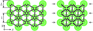
Figure 1: Bead–spring model with hard cores for interacting hard particles at the air/water interface or a liquid interface. The springs give the network a Hookean elasticity, and the hard cores (green disks, diameter $L$) impose limits on the maximal admissible compression (see configuration on the right). The lattice constant is normalized to $1$ and $L<1$.

In order to verify this interpretation, we develop an elasticity model based on the microscopic view of a particle raft sketched in Figure 1: Globular particles interact by soft springs (corresponding to an outer soft shell) and steric interactions (corresponding to hard cores). From this microscopic view, we derive continuum elastic laws, which can then be used to analyze the deflated shapes of capsules with this type of elasticity. The hypothesis underlying this approach is the following: The steep increase in the surface Young or stretch modulus that was obtained in ref 28 is a result of applying linear Hookean elasticity in a situation where the proposed elasticity model for the protein particle raft that includes hard cores should be more appropriate. Therefore, we should be able to describe the observed shapes of hydrophobin-coated bubbles more exactly and with much less variation of the elastic moduli along the deflation trajectory if the new hard-core/soft-shell elasticity model is used.

The proposed elasticity model is quite generic: It is a generalization of a standard bead–spring model for Hookean elastic membranes Seung and Nelson (1988), which also takes into account hard cores of the beads. On the other hand, it generalizes a particle raft elasticity model presented in ref 14, which considers exclusively hard-core interactions. Therefore, our hard-core/soft-shell elasticity model applies more widely than to monolayers of the protein hydrophobin. We expect such contact interaction to be relevant for many liquid interfaces decorated with interacting hard particles Zeng et al. (2006), ranging from colloidal rafts covering colloidosomes Dinsmore et al. (2002) or “armoured droplets” Subramaniam et al. (2005) to rafts of larger particles Vella et al. (2004).

Our results will show that the elastic properties of the two-dimensional material are Hookean for small compression, where only soft springs are loaded without hard-core contact but strongly modify as soon as compression brings the hard cores of particles into contact. The constitutive stress–strain relations of the soft spring, which determine the material properties for small compression, have to be properly connected to stress relations, which are governed by force balance for compressions that induce hard-core contact. The transition between both regimes can take place between different regions within the same material, as we will see in the analysis of shapes of pendant or buoyant capsules attached to a capillary. A detailed and quantitative understanding of shapes and deformations of such compressed particle-decorated liquid interfaces therefore requires a model as presented here, which properly connects Hookean elasticity of soft springs or soft particle interactions with hard-core elasticity, and goes beyond a simple effective description based on Hookean elasticity.

II Continuum Description of a Bead–Spring Model with Hard Cores

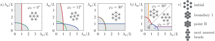
Figure 2: Forbidden domains (light gray) in the $(\lambda_{x},\lambda_{y})$-plane limited by ellipses. (a) Different orientations $\varphi_{0}$ produce different forbidden domains. Straight lines are degenerate ellipses with infinite major axis, and dashed lines with alternating color indicate if two of the three ellipses are identical. The pictograms show the lattice orientation. (b) Choice of $\varphi_{0}$ that minimizes the area of the forbidden domain. For easy identification, the boundaries are labeled 1 and 2; and the point on both lines is termed B. There is an additional vertical and horizontal boundary at $\lambda_{i}/L=1/\sqrt{3}$ where next nearest beads come into contact. (c) Sketches of the different possibilities of contact between the beads, here for $\varphi_{0}=30^{\circ}$, that is, when the compression is predominantly in $x$-direction.

We assume that the beads are arranged in the $(x,y)$-plane in a hexagonal crystal with a lattice constant normalized to $1$, see Figure 1. Such an arrangement is the closest packing of spheres and it behaves isotropically Landau and Lifshitz (1987), so that the continuum elasticity of the membrane can be characterized by two elastic moduli, for example the surface Poisson ratio $\nu$ and surface Young modulus $E_{\text{2D}}$. On the microscopic level, the elastic response of the membrane is governed by the spring constant $k$. By evaluation of the deformation energy within one unit cell, it can be shown that the continuum elastic moduli are determined by Ostoja-Starzewski (2002); Seung and Nelson (1988)

$$E_{\text{2D}}=\frac{2}{\sqrt{3}}\,k\quad\text{and}\quad\nu=\frac{1}{3}.$$ (1)

Without the hard-core interactions, the membrane can thus be described with the usual Hookean elasticity as specified by the strain-energy density Libai and Simmonds (1998)

$$\begin{multlined}w_{S}(\lambda_{x},\lambda_{y})=\frac{1}{2}\frac{E_{\text{2D}}}{1-\nu^{2}}\big{[}(\lambda_{x}-1)^{2}\\ +2\nu(\lambda_{x}-1)(\lambda_{y}-1)+(\lambda_{y}-1)^{2}\big{]}+\lambda_{x}\lambda_{y}\gamma,\end{multlined}w_{S}(\lambda_{x},\lambda_{y})=\frac{1}{2}\frac{E_{\text{2D}}}{1-\nu^{2}}\big{[}(\lambda_{x}-1)^{2}\\ +2\nu(\lambda_{x}-1)(\lambda_{y}-1)+(\lambda_{y}-1)^{2}\big{]}+\lambda_{x}\lambda_{y}\gamma,$$ (2)

where $\lambda_{x}$ and $\lambda_{y}$ denote the stretches in $x$- and $y$-direction, respectively. The strain energy density is measured per surface area of the undeformed interface. The form of the surface energy density in eq 2 is valid only for deformations where the $x$- and $y$-directions are the principal directions of the strain tensor, which we assume throughout this paper. This means that a line element $(\mathrm{d}x_{0},\mathrm{d}y_{0})$ is mapped to $(\mathrm{d}x,\mathrm{d}y)=(\lambda_{x}\mathrm{d}x_{0},\lambda_{y}\mathrm{d}y_{0})$ by the deformation.

The term $\lambda_{x}\lambda_{y}\gamma$ accounts for an isotropic surface tension $\gamma$ acting in the liquid surface Knoche et al. (2013). We assume that the corresponding liquid interface covers the entire deformed area $\lambda_{x}\lambda_{y}A_{0}$, where $A_{0}$ is the undeformed reference interface area. In the presence of adsorbed particles, which are only partially wet, a fixed area $A_{\rm hard}$ of the liquid surface is replaced by a liquid-solid-interface with a surface tension $\gamma_{\rm hard}$, and the last term in eq 2 becomes $(\lambda_{x}\lambda_{y}-A_{\rm hard}/A_{0})\gamma+(A_{\rm hard}/A_{0})\gamma_{\text{hard}}$. This shift by a constant independent of the stretching factors does neither change the interface stresses nor the resulting shape equations.

From the energy density eq 2, the stresses acting in the interface can be derived Libai and Simmonds (1998). A superscript ${}^{(\text{s})}$ indicates that this is the contribution of the springs,

$$\tau^{\smash{(\text{s})}}_{x}(\lambda_{x},\lambda_{y})=\frac{E_{\text{2D}}}{1-\nu^{2}}\frac{1}{\lambda_{y}}\left[(\lambda_{x}-1)+\nu(\lambda_{y}-1)\right]+\gamma,$$ (3)

and with indices $x$ and $y$ interchanged for $\tau^{\smash{(\text{s})}}_{y}$. We note that compression with $\lambda_{i}<1$ gives rise to negative elastic contributions to the stresses, whereas the surface tension $\gamma$ always provides a positive contribution, such that $\tau_{i}\leq\gamma$.

Now we have to evaluate how these results from the spring elasticity are modified by the steric interactions between the hard cores. The springs in the lattice have a rest length of $1$ and can be oriented along three different directions $i$, which we characterize by the angle $\varphi_{i}$ to the $x$-axis. This angle can take the values $\varphi_{i}=\varphi_{0}+i\pi/3$, with $i\in\{-1,0,1\}$, where $\varphi_{0}$ determines the overall orientation of the lattice in the $(x,y)$-plane. Upon deformation, the length of a spring along direction $i$ changes from $1$ to

$$d_{i}=\left|\begin{pmatrix}\lambda_{x}\cos\varphi_{i}\\ \lambda_{y}\sin\varphi_{i}\end{pmatrix}\right|=\sqrt{\lambda_{x}^{2}\cos^{2}\varphi_{i}+\lambda_{y}^{2}\sin^{2}\varphi_{i}}.$$ (4)

The steric interactions enforce that the springs of the lattice can be compressed at maximum to a minimal length of $L$ (with $L<1$), which corresponds to the diameter of the hard cores, measured in units of the lattice constant. Thus, we have three conditions $d_{i}\geq L$ to be satisfied, or equivalently

$$\lambda_{x}^{2}\,\cos^{2}(\varphi_{0}-\pi/3)+\lambda_{y}^{2}\,\sin^{2}(\varphi_{0}-\pi/3) \geq L^{2}$$ (5)

$$\lambda_{x}^{2}\,\cos^{2}(\varphi_{0})+\lambda_{y}^{2}\,\sin^{2}(\varphi_{0}) \geq L^{2}$$

$$\lambda_{x}^{2}\,\cos^{2}(\varphi_{0}+\pi/3)+\lambda_{y}^{2}\,\sin^{2}(\varphi_{0}+\pi/3) \geq L^{2}.$$

In the $(\lambda_{x},\lambda_{y})$-plane, these conditions specify three ellipses to be excluded from the admissible domain for the stretches; see Figure 2a. All three ellipses contain the point $(L,L)$.

The excluded or “forbidden” domain of stretches, shaded light gray in Figure 2a and b, depends on the orientation $\varphi_{0}$ of the lattice. We choose this parameter according to the following rule: If $\lambda_{x}<\lambda_{y}$, then $\varphi_{0}=30^{\circ}$; otherwise $\varphi_{0}=0^{\circ}$. With this choice, the forbidden domain becomes as small as possible; see Figure 2b. Choosing $\varphi_{0}$ in dependence of the stress state means that it may change during a deformation; for particle rafts this seems plausible because the particles are not rigidly cross-linked, but may rearrange to change their lattice orientation from a $0^{\circ}$ to a $30^{\circ}$ state (see pictograms in Figure 2c). If the stress state of the membrane becomes inhomogeneous, as it will happen, for example, for capsules attached to a capillary as considered below in more detail, we may encounter regions of $0^{\circ}$ and $30^{\circ}$ orientation within a single membrane. Then, problems might arise at the boundary separating two regions of different orientation, because the lattices cannot be joined properly. This could give rise to a line energy; we neglect these complications in the following.

With our choice of $\varphi_{0}$, the boundary line between the forbidden and admissible domain of the stretch plane can be described by $(\lambda^{\smash{(\text{b})}}_{x},\lambda^{\smash{(\text{b})}}_{y})=(\lambda^{\smash{(\text{b})}}_{x}(\lambda_{y}),\lambda_{y})$ with

$$\lambda^{\smash{(\text{b})}}_{x}(\lambda_{y})=\begin{cases}\sqrt{4L^{2}/3-\lambda_{y}^{2}/3}&\text{if }\lambda_{y}>L\text{ (boundary 1)}\\ \sqrt{4L^{2}-3\lambda_{y}^{2}}&\text{if }\lambda_{y}<L\text{ (boundary 2)}.\end{cases}$$ (6)

Here we have introduced the terms boundary 1 and 2, which have to be distinguished in most of the following calculations. They are plotted in red and blue, respectively, in Figure 2b. The point $(\lambda_{x},\lambda_{y})=(L,L)$ which is on both boundary lines is termed point B.

If the external loads try to push the membrane into the forbidden domain, the hard-core interactions keep it on the boundary by providing additional contributions to the stresses $\tau_{x}$ and $\tau_{y}$. These hard-core contributions are denoted by $\tau^{\smash{(\text{c})}}_{x}$ and $\tau^{\smash{(\text{c})}}_{y}$. The complete stresses then read

$$\tau_{x}=\tau^{\smash{(\text{s})}}_{x}(\lambda_{x},\lambda_{y})+\tau^{\smash{(\text{c})}}_{x}\quad\text{and}\quad\tau_{y}=\tau^{\smash{(\text{s})}}_{y}(\lambda_{x},\lambda_{y})+\tau^{\smash{(\text{c})}}_{y}$$ (7)

with $(\lambda_{x},\lambda_{y})$ being a point on the boundary of the forbidden domain as given by eq 6. Since $\tau^{\smash{(\text{c})}}_{x}$ and $\tau^{\smash{(\text{c})}}_{y}$ are transmitted through the “skeleton” of hard cores, they must satisfy certain conditions of force equilibrium that can be derived from the geometry of the lattice. In Appendix A, it is shown that force balance prescribes the ratio of the hard-core stresses to

$$\frac{\tau^{\smash{(\text{c})}}_{y}}{\tau^{\smash{(\text{c})}}_{x}}=\begin{cases}{\lambda_{y}^{2}}/3{\lambda_{x}^{2}}&\text{if }\lambda_{y}>L\text{ (boundary 1)}\\ 3{\lambda_{y}^{2}}/{\lambda_{x}^{2}}&\text{if }\lambda_{y}<L\text{ (boundary 2)}\end{cases}$$ (8)

$$\text{and}\quad\frac{1}{3}\leq\frac{\tau^{\smash{(\text{c})}}_{y}}{\tau^{\smash{(\text{c})}}_{x}}\leq 3\quad\text{if }\lambda_{x}=\lambda_{y}=L\text{ (point B)}.$$

Note that $(\lambda_{x},\lambda_{y})$ must always be a point on the boundary of the forbidden domain when these equations are applied to calculate the hard-core contributions to the stresses.

For strong compressive strains with $\lambda_{x}<1/\sqrt{3}$ or $\lambda_{y}<1/\sqrt{3}$, next nearest beads, which are not connected by springs, come into contact; see Figure 2b, orange and violet lines. Such compressive strains are not relevant for the applications discussed in this Article.

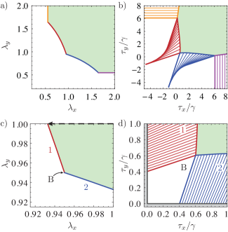
Figure 3: Admissible domains (light green) and hard-core interaction domains for stretches (a, c) and stresses (b, d) for $L=0.95$ and $E_{\text{2D}}=5\gamma$. The top row shows large views of the stress and stretch planes, and the bottom row close-ups of the relevant region. In (b) and (d), the straight thin lines indicate the stresses that can be reached from a point on the boundary by adding the hard-core contributions to the elastic stresses. The wrinkling region is shaded in gray in (d). The arrow in (c) indicates the trajectory of uniaxial compression of a planar layer considered below.

The above results for our custom elasticity model for particle rafts are summarized and illustrated in Figure 3. Figure 3a and b shows a large view of the stretch plane and stress plane with different regions. Figure 3c and d focuses on the regime relevant for compressed membranes: $\lambda_{i}\leq 1$ and $0<\tau_{i}\leq\gamma$. The light green regions are the admissible regions, where the hard cores are not in contact. Here, the usual Hookean elasticity (eq 3) is valid, and there is a bijective mapping between $(\lambda_{x},\lambda_{y})$ points in the stretch plane and $(\tau_{x},\tau_{y})$ points in the stress plane.

On boundaries 1 and 2, the hard cores come into contact. In the stretch plane, this boundary cannot be trespassed because of the geometric constraints imposed by the undeformable hard cores: Even if the external forces try to push the lattice beyond this line, the lattice will get stuck on the boundary of the forbidden domain. In the stress plane, however, the points beyond boundaries 1 and 2 can be accessed by including the hard-core contributions $\tau^{\smash{(\text{c})}}_{x}$ and $\tau^{\smash{(\text{c})}}_{y}$ in the stresses because hard cores can transmit force even though they are undeformable.

A point $\big{(}\lambda^{\smash{(\text{b})}}_{x},\lambda^{\smash{(\text{b})}}_{y}\big{)}$ on the boundary in the stretch space is mapped by Hooke’s law to a point $\big{(}\tau^{\smash{(\text{b})}}_{x},\tau^{\smash{(\text{b})}}_{y}\big{)}$ on the boundary in the stress space. From this point on, stresses $(\tau_{x},\tau_{y})=\big{(}\tau^{\smash{(\text{b})}}_{x},\tau^{\smash{(\text{b})}}_{y}\big{)}+\big{(}\tau^{\smash{(\text{c})}}_{x},\tau^{\smash{(\text{c})}}_{y}\big{)}$ can be reached, where the hard-core contributions $\tau^{\smash{(\text{c})}}_{x}$ and $\tau^{\smash{(\text{c})}}_{y}$ must be negative (because the skeleton can only support compressive stresses) and must obey the force balance constraint (eq 8). The submanifold of stresses which is accessible from the point on the boundary is, thus, a straight line with a slope $\lambda_{y}^{2}/3\lambda_{x}^{2}$ starting from boundary 1 or $3\lambda_{y}^{2}/\lambda_{x}^{2}$ starting from boundary 2 in Figure 3d (see the thin red and blue lines). The analogous discussion of the boundaries where next nearest beads come into contact is spared because it is not relevant for the applications presented below.

For point B, with $\lambda_{x}=\lambda_{y}=L$, the ratio of the hard-core stresses is not fixed to a certain value. Instead, it can range from $1/3$ to $3$. In the plot of the stress plane, Figure 3d, this means that the whole white region is accessible from point B.

III Compression of Planar Films

To get a first impression of the elastic behaviour of a particle layer with hard cores at a fluid interface, we investigate a typical compression experiment in a Langmuir trough Cicuta and Vella (2009); Aumaitre et al. (2011). In this setup, a monolayer is spread on a water surface and subsequently it is compressed in $x$-direction by moving the barriers of the trough. A Wilhelmy plate can then measure the stresses $\tau_{x}$ and $\tau_{y}$.

If we consider $\lambda_{y}=1$ as fixed and compress the layer with a ratio $\lambda_{x}<1$, we expect the monolayer to wrinkle at sufficiently high compression. The determination of the critical compression is a purely geometric problem. In the stretch space of Figure 3c, we follow a horizontal line until we cross boundary 1 as indicated by the arrow. Then the layer must wrinkle because the hard cores cannot be compressed.

On the other hand, if we consider the compressive stress $\tau_{x}<0$ to be given, we can determine the critical stress from the stability equation Vella et al. (2004); Landau and Lifshitz (1970)

$$E_{B}\partial_{x}^{4}w(x)-\tau_{x}\partial_{x}^{2}w(x)+\rho gw(x)=0,$$ (9)

where $E_{B}$ is the bending stiffness of the layer, $w(x)$ is the displacement in the $z$-direction which is assumed to be independent of $y$, and $\rho g$ is the fluid density times acceleration of gravity. The bending rigidity $E_{B}$ can arise from an additional bending stiffness of connecting springs. For hydrophobin layers this corresponds to a bending rigidity of the soft shell of the protein. Assuming sinusoidal wrinkles of the form $w\sim\sin kx$, eq 9 gives a critical stress $\tau_{x}$ which still depends on the wavenumber $k$ of our ansatz. Minimizing the magnitude of the stress with respect to $k$ gives a critical wavelength and critical stress of Vella et al. (2004)

$$\lambda_{c}=2\pi\left(E_{B}/\rho g\right)^{1/4}\quad\text{and}\quad\tau_{x,c}=-2\sqrt{E_{B}\rho g}.$$ (10)

This is the same result as that for an elastic membrane without hard cores. The result for $\lambda_{c}$ differs from what has been obtained in ref 14: we do not find a dependence on the packing fraction of hard particles because the bending modulus corresponding to the soft springs appears in eq 10 rather than an effective modulus depending on packing fraction as in ref 14.

Differences between membranes with and without hard cores can be found when the Poisson ratio of the layer is measured. For uniaxial compressive strain in the $x$-direction ($\lambda_{x}<1$, $\lambda_{y}=1$), the Poisson ratio of a linear elastic material can be measured as $\nu=\tau_{y}/\tau_{x}$. Now let us apply this “measurement” to the more complex total stresses in eq 7:

$$\nu_{\text{app}}=\frac{\tau^{\smash{(\text{s})}}_{y}+\tau^{\smash{(\text{c})}}_{y}-\gamma}{\tau^{\smash{(\text{s})}}_{x}+\tau^{\smash{(\text{c})}}_{x}-\gamma}=\frac{\Pi_{y}}{\Pi_{x}}.$$ (11)

Here, we subtract the fluid surface tension $\gamma$ from the total stresses, which provides a background tension and is typically subtracted in measurements of the surface pressures $\Pi_{x}$ and $\Pi_{y}$ Cicuta and Vella (2009); Aumaitre et al. (2011). For simplicity, we also neglect the $1/\lambda_{x}$ prefactor in relation (3) for $\tau^{\smash{(\text{s})}}_{y}$, which represents a geometrical nonlinearity. In the regime where the hard cores are in contact, the apparent Poisson ratio thus reads

$$\nu_{\text{app}}=\frac{\frac{\nu}{1-\nu^{2}}(\lambda^{\smash{(\text{b})}}_{x}-1)+\tilde{\tau}^{\smash{(\text{c})}}_{x}/3(\lambda^{\smash{(\text{b})}}_{x})^{2}}{\frac{1}{1-\nu^{2}}(\lambda^{\smash{(\text{b})}}_{x}-1)+\tilde{\tau}^{\smash{(\text{c})}}_{x}}$$ (12)

with $\lambda^{\smash{(\text{b})}}_{x}=\sqrt{4L^{2}/3-1/3}$ and $\tilde{\tau}^{\smash{(\text{c})}}_{x}=\tau^{\smash{(\text{c})}}_{x}/E_{\text{2D}}$. The hard cores have a nonvanishing contribution $\tilde{\tau}^{\smash{(\text{c})}}_{x}$ only if the applied compressive stress satisfies $\tau_{x}<\frac{E_{\text{2D}}}{1-\nu^{2}}(\lambda^{\smash{(\text{b})}}_{x}-1)$ so that the hard cores are in contact. For larger $\tau_{x}$ or weak compression, the usual Hookean law is valid, which leads to $\nu_{\text{app}}=\nu=1/3$. In the limit of strong compression where the hard-core contribution dominates the stresses, we have $\nu_{\text{app}}=1/3(\lambda^{\smash{(\text{b})}}_{x})^{2}=1/(4L^{2}-1)$, which is always larger than $1/3$ for $L<1$ and can even become larger than $1$. For $L<1/\sqrt{3}$, this relation changes because next nearest beads come into contact. This shows that contact of hard cores can give rise to a more effective redirection of compressive stress into the perpendicular direction, which gives rise to a stress-dependent Poisson ratio increasing with compression. The crossover between weak compression with the Hookean value $\nu=1/3$ and the increasing apparent Poisson ratio $\nu_{\text{app}}$ for strong compression is shown in Figure 4 for different values of $L$. Our results differ from $\nu_{\text{app}}=1/\sqrt{3}$, which has been found in ref 14 for pure hard-core particle rafts. In ref 36, on the other hand, it has been argued that $\nu_{\text{app}}=1/3$ is correct also for pure hard-core particle rafts. Our result (eq 12) for the more general elasticity model explains that, for rafts of interacting hard particles, where the interaction provides a “soft shell”, experimental measurements such as those in refs 33 and 37 should be interpreted using a stress-dependent Poisson ratio, which increases beyond $1/3$ and up to $\nu_{\text{app}}=1/(4L^{2}-1)$ if hard cores come into contact; see Figure 4.

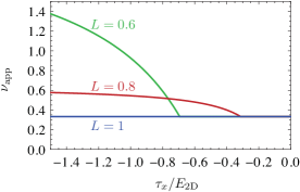
Figure 4: Apparent Poisson ratio $\nu_{\text{app}}={\Pi_{y}}/{\Pi_{x}}$ in our elasticity model for different values of $L$ as indicated. At the kinks, the hard cores come into contact and the hard-core contributions to the stresses begin to influence this “measured” Poisson ratio.

In ref 37, for example, an experiment is reported where a monolayer of hydrophobin molecules is compressed in a Langmuir trough. Two Wilhelmy plates were used to measure the stresses in $x$- and $y$-directions, respectively, and from the data one can calculate an apparent Poisson ratio of $\nu_{\text{app}}\approx 0.6-0.7$. This relatively large value can be well explained with our elasticity model if $L\lesssim 0.8$ according to Figure 4. It is tempting to compare this hard-core length to available molecular information. In ref 34, it has been observed that visual buckling, which could be due to hard-core contact, happens at a molecular area of $a_{\rm buckle}\approx 347\,{\mbox{\AA}}^{2}$ per HFBII hydrophobin protein. Assuming closed-packed hard cores, this corresponds to a diameter of $20\,{\mbox{\AA}}$, if HFBII is assumed to be spherical. A value $L=0.8$ then corresponds to a total diameter of $25\,{\mbox{\AA}}$ of the protein. This value is consistent, for example, with the dimensions $24\times 27\times 30\,{\mbox{\AA}}$ given for the whole HFBII molecule as obtained from X-ray crystallography Hakanpää et al. (2004). Grazing-incidence X-ray diffraction and reflectivity results in ref 38 hint, however, at smaller diameters $20-24\,{\mbox{\AA}}$ and, thus, larger values of $L$. In refs 37 and 39, plateaus in the surface pressure isotherms have been observed, which can be interpreted as a liquid–gas coexistence of a gas phase of isolated hydrophobins and a dilute liquid where soft shells of hydrophobins just start to make contact. Taking the area per molecule $a_{\rm plateau}$ at the high-density end of these plateaus we find values of $L=(a_{\rm plateau}/a_{\rm buckle})^{1/2}$ in the range $L=0.85-0.90$. Overall, a reliable estimate of $L$ based on molecular information appears difficult.

IV Shape Equations in the Pendant/Rising Capsule Geometry

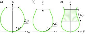
Figure 5: Arc-length parametrizations in cylindrical coordinates of the undeformed $(r_{0}(s_{0}),z_{0}(s_{0}))$, deformed $(r(s),z(s))$ and the wrinkled midsurface. The wrinkled region of length $L_{w}$ is described by an axisymmetric pseudosurface around which the real midsurface oscillates.

We now apply the previously developed elasticity model to the shape equations for axisymmetric capsules attached to a capillary which have been developed in ref 28. This is a challenging problem because it turns out that the transition between the elasticity regimes A, 1, 2, and B can take place within the same material between different axisymmetric regions along the capsule. Therefore, we have to generalize the shape equations from ref 28 to include switching between different constitutive elastic laws corresponding to the Hookean regime A and the hard-core dominated regimes 1, 2, and B along the capsule contour.

The shape equations are derived from non-linear shell theory and their solution describes the shape and stress distribution of a deformed pendant or rising capsule. Figure 5 shows the parametrization of the undeformed and deformed capsule shape. At its upper rim, the capsule is attached to a capillary of diameter $a$. The reference shape (see Figure 5a) is a solution of the Laplace-Young equation with an isotropic interfacial tension $\gamma$ and a density difference $\Delta\rho$ of inner and outer fluid Knoche et al. (2013). This shape can be deformed, for example by reducing the internal capsule volume. Each point $(r_{0}(s_{0}),z_{0}(s_{0}))$ is mapped onto a point $(r(s_{0}),z(s_{0}))$ in the deformed configuration, which induces a meridional and circumferential stretch, $\lambda_{s}=\mathrm{d}s/\mathrm{d}s_{0}$ and $\lambda_{\varphi}=r/r_{0}$, respectively. The arc length element $\mathrm{d}s$ of the deformed configuration is defined by $\mathrm{d}s^{2}=(r^{\prime}(s_{0})^{2}+z^{\prime}(s_{0})^{2})\mathrm{d}s_{0}^{2}$.

The shape equations that determine the deformed configuration describe force and torque balance within the capsule shell and are given by Knoche et al. (2013)

$$r^{\prime}(s_{0}) =\lambda_{s}\cos\psi$$ (13)

$$z^{\prime}(s_{0}) =\lambda_{s}\sin\psi$$

$$\psi^{\prime}(s_{0}) =\frac{\lambda_{s}}{\tau_{s}}(p-\Delta\rho\,g\,z-\kappa_{\varphi}\tau_{\varphi})$$

$$\tau_{s}^{\prime}(s_{0}) =\lambda_{s}\frac{\tau_{\varphi}-\tau_{s}}{r}\cos\psi.$$

Here, $\psi$ denotes the slope angle as defined in Figure 5, $\tau_{s}$ and $\tau_{\varphi}$ are the meridional and circumferential stress, respectively, $\kappa_{\varphi}=\sin\psi/r$ is the circumferential curvature, and $p-\Delta\rho\,g\,z$ is the hydrostatic pressure difference exerted on the capsule membrane. In this formulation, the bending stiffness has been neglected since the typical capsules used for these experiments are very thin and bendable Knoche et al. (2013).

In order to solve this system of ordinary differential equations numerically with a shooting method, the quantities $\lambda_{s}$ and $\tau_{\varphi}$ occurring on the right-hand side of the system must be calculated for given $\lambda_{\varphi}$ and $\tau_{s}$ by virtue of an elastic constitutive law. For the simple Hookean elastic law in eq 3 this was demonstrated in ref 28,

$$\lambda_{s} =\frac{1-\nu^{2}}{E_{\text{2D}}}\,\lambda_{\varphi}\,(\tau_{s}-\gamma)-\nu(\lambda_{\varphi}-1)+1,$$ (14)

$$\tau_{\varphi} =\frac{E_{\text{2D}}}{1-\nu^{2}}\,\frac{1}{\lambda_{s}}\big{(}(\lambda_{\varphi}-1)+\nu\,(\lambda_{s}-1)\big{)}+\gamma.$$

The boundary conditions for the system of shape equations are $r(0)=z(0)=\psi(0)=0$ and $r(L_{0})=a/2$, where $L_{0}$ is the contour length in the undeformed configuration and the end-point of the integration. The starting value $\tau_{s}(0)$ is free and serves as a shooting parameter to satisfy the boundary condition at $L_{0}$ Knoche et al. (2013).

Here, we want to use the elasticity model for particle rafts developed above (eqs 3, 7 and 8), including the hard-core interactions. Therefore, depending on the size of compressive stresses, we have to switch between different constitutive elastic relations corresponding to Hookean constitutive relations or hard-core constitutive relations along the arc-length coordinate $s_{0}$ as explained in detail in Appendix B.

IV.1 Wrinkling and Modified Shape Equations

In our model, we neglect the bending stiffness of the capsule membrane. The fact that the membrane is infinitely easy to bend implies that it will immediately wrinkle under compressive stresses. In ref 28, it was shown that deflated pendant capsules exhibit wrinkles due to a compressive hoop stress $\tau_{\varphi}<0$, as also indicated in Figure 5c. The capsule membrane is not axisymmetric in the wrinkled region, but can be approximated by an axisymmetric pseudosurface around which the real membrane oscillates. The shape of this pseudosurface is determined by setting $\tau_{\varphi}=0$ where the original shape equations predict negative hoop stresses. The assumption $\tau_{\varphi}=0$ on the pseudosurface is common to various theories of wrinkling, for example tension field theory Steigmann (1990) or far-from-threshold theory Davidovitch et al. (2011). This leads to a modified system of shape equations

$$\bar{r}^{\prime}(s_{0}) =\lambda_{s}\cos\psi$$ (15)

$$z^{\prime}(s_{0}) =\lambda_{s}\sin\psi$$

$$\psi^{\prime}(s_{0}) =\frac{\lambda_{s}}{\bar{\tau}_{s}}(p-\Delta\rho\,g\,z)$$

$$\bar{\tau}_{s}^{\prime}(s_{0}) =-\lambda_{s}\frac{\bar{\tau}_{s}}{\bar{r}}\cos\psi$$

where $\bar{r}$ is the radial coordinate of the pseudo-surface and $\bar{\tau}_{s}$ the meridional stress measured per unit length of the pseudosurface, that is $\bar{\tau}_{s}=\tau_{s}\lambda_{\varphi}/\bar{\lambda}_{\varphi}$ when $\bar{\lambda}_{\varphi}=\bar{r}/r_{0}$ denotes the pseudo hoop stretch. The system is closed by the equation

$$\lambda_{s}=\frac{\bar{\tau}_{s}\bar{\lambda}_{\varphi}+E_{\text{2D}}-\gamma(1+\nu)}{E_{\text{2D}}-2\nu\gamma-\gamma^{2}(1-\nu^{2})/E_{\text{2D}}}.$$ (16)

A discussion of these modified shape equations for the pseudo-surface and the automatic switching between normal and modified shape equations during the integration can be found in ref 28.

Wrinkling can also occur when the lattice is jammed on boundary 2 or point B. As in ref 28, we handle wrinkling by introducing a pseudosurface (indicated with an overbar) and setting the hoop stress to zero. On boundary 2, we have $\lambda_{\varphi}=\sqrt{4L^{2}/3-\lambda_{s}^{2}/3}$ (note that $\lambda_{\varphi}$ refers to the hoop stretch of the real, wrinkled surface and is to be distinguished from the pseudo hoop stretch $\bar{\lambda}_{\varphi}=\bar{r}/r_{0}$). The condition $\tau_{\varphi}=0$ is equivalent to

$$\tau^{\smash{(\text{c})}}_{\varphi}=-\gamma-\frac{E_{\text{2D}}}{1-\nu^{2}}\frac{1}{\lambda_{s}}\left[\big{(}\lambda_{\varphi}-1\big{)}+\nu(\lambda_{s}-1)\right].$$ (17)

We further have $\tau^{\smash{(\text{c})}}_{s}=\tau^{\smash{(\text{c})}}_{\varphi}\cdot\lambda_{s}^{2}/3\lambda_{\varphi}^{2}$. So the complete meridional tension, measured per unit length of the pseudosurface, is determined by

$$\bar{\tau}_{s}=\frac{\lambda_{\varphi}}{\bar{\lambda}_{\varphi}}\left[\tau^{\smash{(\text{s})}}_{s}(\lambda_{s},\lambda_{\varphi})+\frac{1}{3}\frac{\lambda_{s}^{2}}{\lambda_{\varphi}^{2}}\,\tau^{\smash{(\text{c})}}_{\varphi}\right].$$ (18)

This is a quite complicated function of $\lambda_{s}$, because $\tau^{\smash{(\text{c})}}_{\varphi}$ and $\lambda_{\varphi}$ herein also depend on $\lambda_{s}$. It must be solved for $\lambda_{s}$ to evaluate the right-hand side of the shape equations (eq 15), which is done numerically in each integration step of the shape equations.

When wrinkling occurs in point B, the shape equations for the pseudosurface (eq 15) can also be used, and since $\lambda_{s}=\lambda_{\varphi}=L$, the inversion of a stress–strain relation to obtain $\lambda_{s}$ is not necessary. In point B, the hard-core stresses $\tau^{\smash{(\text{c})}}_{s}$ and $\tau^{\smash{(\text{c})}}_{\varphi}$ are independent of each other, and the spring contributions $\tau^{\smash{(\text{s})}}_{s}$ and $\tau^{\smash{(\text{s})}}_{\varphi}$ are fixed because of $\lambda_{s}=\lambda_{\varphi}=L$. From the wrinkling condition $\tau_{\varphi}=0$ we can, thus, calculate $\tau^{\smash{(\text{c})}}_{\varphi}$. The meridional hard-core contribution $\tau^{\smash{(\text{c})}}_{s}$ must be calculated from the differential equation for $\tau_{s}$. Note that the geometry of the pseudosurface is not fixed by the condition $\lambda_{s}=\lambda_{\varphi}=L$ because the circumferential stretch $\bar{\lambda}_{\varphi}$ of the pseudosurface is free. This is in contrast to the case of a lattice being stuck in point B without wrinkling as discussed above.

IV.2 Numerical Integration and Switching between the Shape Equations

The modified shape equations are integrated from the apex $s_{0}=0$ to the attachment point $s_{0}=L_{0}$ to the capillary. On this way, the integration will run through different domains and must switch to the appropriate shape equations discussed in the previous section and Appendix B. Figure 6 shows typical trajectories of the integration in the stress plane, that is, parametric plots of $(\tau_{s}(s_{0}),\tau_{\varphi}(s_{0}))$ with $s_{0}\in[0,L_{0}]$.

We name the different domains of the stress plane as follows: The admissible domain (light green in Figure 6) is abbreviated “A”, the red and blue ruled regions are termed “1” and “2” (because they stem from boundary 1 and 2 in the stretch plane), and the white region is termed “B”. Regions 2 and B also appear in wrinkled form, and we then call them “2W” and “BW”.

In the numerical integration, an event handler must be introduced which detects when the integration runs from one region into another. Changes from region A to regions 1, 2 or B can be detected on the basis of strains, which are limited by the boundary of the forbidden domain as given by eq 6. The other direction, a change from a hard-core region into the A domain, occurs when the hard-core stresses become positive.

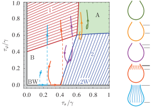
Figure 6: Trajectories in the stress plane for integrations at different stages of deflation (see pictograms on the right). Thin dashed parts of the trajectories are jumps in $\tau_{\varphi}$. The integration always starts at the apex with $\tau_{s}=\tau_{\varphi}$, that is, on the angle bisector, and runs through different domains of the stress plane. The parameters of the elastic model are $E_{\text{2D}}/\gamma=5$, $\nu=1/3$, and $L=0.95$. In the pictograms, thin horizontal lines indicate the transitions between the regions.

Switching between the different hard-core regions is, however, a bit more complicated because the continuity conditions are less obvious. An elaborate variational calculation Knoche (2014) shows surprisingly that $\tau_{\varphi}$ may jump at transitions from B$\,\rightarrow\,$BW, B$\,\rightarrow\,$2, 2$\,\rightarrow\,$1 and BW$\,\rightarrow\,$1; see also Figure 6. The physical reason behind this behavior is that $\tau_{\varphi}$ is constitutively undetermined in region B: It may jump without requiring the hoop stretch $\lambda_{\varphi}$ to jump, which would be unphysical and would lead to a ruptured shape. This jump is necessary when starting in region B, where we see in Appendix B that the shooting parameter is eliminated: The jump, or rather its arc-length coordinate $s_{J}$, serves as a substitute shooting parameter. In the following discussion of each trajectory shown in Figure 6, this becomes more clear.

B$\,\boldsymbol{\rightarrow}\,$BW$\,\boldsymbol{\rightarrow}\,$1, Light Blue.

The transition from B to BW occurs at $s_{J}$ which can be chosen arbitrary (it just has to occur before the trajectory reaches the wrinkling region $\tau_{\varphi}=0$). This is the shooting parameter that is adjusted to match the boundary condition $r(L_{0})=a/2$ at the end of integration. The rest of the trajectory follows from the rules formulated above: The jump from BW to 1 occurs when the wrinkling condition $\bar{\lambda}_{\varphi}\leq\lambda_{\varphi}$ becomes false. As the stretches are fixed to $L$ in B, BW and on the boundary of 1, the stretches are continuous at this transition, only the hoop stress jumps.

B$\,\boldsymbol{\rightarrow}\,$BW$\,\boldsymbol{\rightarrow}\,$2W$\,\boldsymbol{\rightarrow}\,$2$\,\boldsymbol{\rightarrow}\,$1, Light Red.

The first transition occurs again at a free position $s_{J}$, and the remainder of the course follows: BW$\,\rightarrow\,$2W is continuous and occurs when the ratio $\tau^{\smash{(\text{c})}}_{\varphi}/\tau^{\smash{(\text{c})}}_{s}$ becomes larger than 3; 2W$\,\rightarrow\,$2 is also continuous and happens when $\bar{\lambda}_{\varphi}$ becomes larger than $\lambda_{\varphi}$; and 2$\,\rightarrow\,$1, which has a jump in $\tau_{\varphi}$, is determined by $\lambda_{\varphi}$ becoming larger than $L$.

B$\,\boldsymbol{\rightarrow}\,$2$\,\boldsymbol{\rightarrow}\,$1, Violet.

Again, the transition out of region B happens at a shooting parameter $s_{J}$, and the second transition follows as explained in the previous trajectory.

A$\,\boldsymbol{\rightarrow}\,$2$\,\boldsymbol{\rightarrow}\,$A, Dark Yellow.

For this trajectory, the shooting parameter is $\tau_{s}(0)$ as usual, because we are starting in region A. The integration switches from A to 2 when the boundary in the stretch plane is reached according to eq 6; and back to A when the hard-core stresses become positive. Both transitions are continuous. A transition from A to 1 is also possible and obeys the same reasoning.

The dark green trajectory is trivial because it stays in region A for the whole integration. More paths are possible and have been worked out, but the presented ones were most commonly met in the numerical investigations.

V Analysis of Computed Deflated Shapes

With the newly developed shape equations, we can compute deflated shapes of capsules according to the hard-core/soft-shell elasticity model. For the numerical analysis, we use $\gamma$ as the tension unit and $a$ as the length unit. Dimensionless quantities are denoted with a tilde. Specifically, the shape equations depend on the reduced density difference $\tilde{\rho}=a^{2}\Delta\rho g/\gamma$, the reduced pressure $\tilde{p}=ap/\gamma$ which controls the capsule volume and the reduced surface Young modulus $\tilde{E}_{\text{2D}}=E_{\text{2D}}/\gamma$. Their dimensionless solutions contain the shape $(\tilde{r},\tilde{z})=(r/a,z/a)$ and tensions $\tilde{\tau}_{i}=\tau_{i}/\gamma$ with $i\in\{s,\varphi\}$.

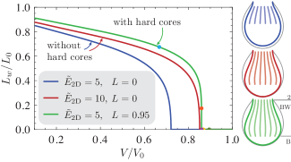
Figure 7: Wrinkle length as a function of the reduced volume for deflated shells with and without hard-core interactions, for $\nu=1/3$ and $\tilde{E}_{\text{2D}}$ as indicated in the legend. The shapes on the right for $V=0.7V_{0}$ reveal differences not only in $L_{w}$ but also in the overall shape (colors as in the legend, thin gray line is the undeformed shape, integration regions are indicated in the green contour). The five data points on the green line in the diagram indicate the shapes and trajectories shown in Figure 6.

Starting with a Laplace-Young shape Knoche et al. (2013) with $\tilde{\rho}=0.25$ and $\tilde{p}_{0}=2$, the pressure is lowered from $\tilde{p}=\tilde{p}_{0}$ to $\tilde{p}=0.1\tilde{p}_{0}$. Figure 7 shows the arc length $L_{w}$ of the wrinkled region as a function of the reduced volume for three such series of deflated shapes with different elastic parameters. The curves without hard-core interactions (red and blue, with $L=0$) show that the onset of wrinkling occurs earlier for higher elastic moduli. If hard-core interactions are included and occur already for small compressions (green curve, $L=0.95$), the wrinkling sets in early, even though the elastic modulus is small. Here, the wrinkling is induced by hard cores coming into contact. After hard-core contact, compressive stresses increase much more quickly with decreasing volume, as it can also be seen in the larger “stress loops” in regions 1, 2, and B in the trajectories shown in Figure 6. If these stress loops touch the gray shaded wrinkling regions, wrinkling is triggered (red and blue shapes in Figure 6). The quickly increasing stress loops after hard-core contact also give rise to the rather steep increase of the arc length $L_{w}$ of the wrinkled region as a function of the reduced volume in the corresponding green line in Figure 7.

Thus, if one analyzes the shape of a deflated capsule, not knowing that it obeys the hard-core/soft-shell elasticity model but assuming that it is a usual Hookean membrane, the Hookean elastic modulus will be overestimated considerably. Figure 7 illustrates this, as the green line with $\tilde{E}_{\text{2D}}=5$ and $L=0.95$ is much closer to the red line with $\tilde{E}_{\text{2D}}=10$ than to the blue line with $\tilde{E}_{\text{2D}}=5$.

V.1 Shape Analysis of Theoretically Generated Shapes

In ref 28, a shape analysis for deflated pendant capsules was developed. From experimental images, the contours are extracted and fitted with the solutions of the shape equations (eqs 13). This allows one to determine the elastic modulus of the capsule membrane. The application of this method to bubbles coated with a layer of the protein hydrophobin revealed a very nonlinear elastic behavior, and the fitted elastic modulus as a function of the volume jumps at the onset of wrinkling. The essential features of the Hookean elastic modulus obtained in ref 28 are shown in Figure 8b, where the area compression modulus $K_{\text{2D}}=E_{\text{2D}}/2(1-\nu)$ is used instead of the surface Young modulus.

We test whether this characteristic signature of the hydrophobin layer elasticity can be explained by our hard-core/soft-shell elasticity model. To this end, series of deflated shapes are computed using our modified shape equations for a given area compression modulus $\tilde{K}_{\text{orig}}$ for the soft springs and a given hard-core length $L$. Then each theoretically generated shape is converted into a set of sampling points and fed to the usual shape analysis algorithm developed in ref 28 which uses a Hookean elasticity model without hard cores. The output of the shape analysis algorithm is a fitted Hookean area compression modulus $\tilde{K}_{\text{2D}}$ for each capsule volume, which is shown in Figure 8a1-a5 and demonstrates that the fitted Hookean area compression modulus $\tilde{K}_{\text{2D}}$ can differ substantially from the value $\tilde{K}_{\text{orig}}$ of the soft springs that has been used for the theoretical shape generation and that the fitted Hookean area compression modulus can change with volume although $\tilde{K}_{\text{orig}}$ and the hard-core length $L$ are fixed. In principle, the shape analysis algorithm using Hookean elasticity can also also give a fit value for the Poisson ratio $\nu$. Alternatively, we can fix $\nu$ in the fit procedure to reduce the number of free parameters.

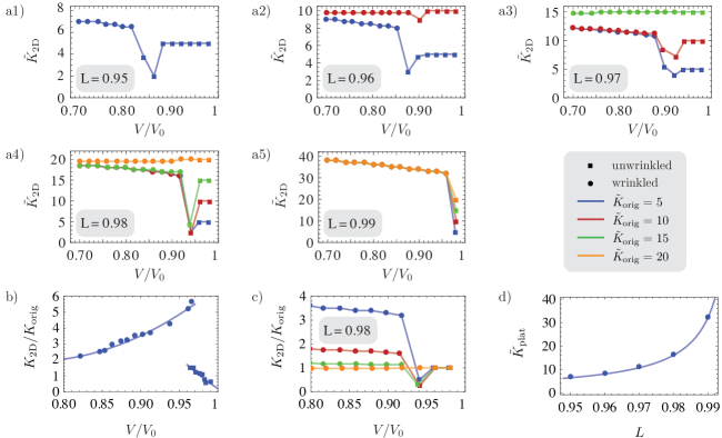
Figure 8: (a1–a5) Fit results for theoretically generated capsule shapes of various area compression moduli $\tilde{K}_{\text{orig}}$ of the soft shells and hard-core lengths $L$. The fits are performed using the usual Hookean elasticity (without hard cores) and come to differing results $\tilde{K}_{\text{2D}}$ for the fitted Hookean area compression modulus. In both shape generation and fits, the Poisson ratio is fixed to $\nu=1/3$. Shapes exhibiting wrinkling are indicated by circles, unwrinkled shapes by squares. (b) Typical fit results for the dimensionless $\tilde{K}_{\text{2D}}/\tilde{K}_{\text{orig}}$ area compression modulus of a hydrophobin capsule as obtained in ref 28. The jump in the elastic modulus coincides with the onset of wrinkling. (c) Fit results to theoretically generated capsule shapes from subfigure (a4), normalized to $K_{\text{orig}}$. (d) The relation between the plateau value $\tilde{K}_{\text{plat}}$ of the fitted Hookean modulus $\tilde{K}_{\text{2D}}$ and the hard-core length $L$ according to subfigures (a1)–(a5).

The analysis is concentrated to soft shell area compression moduli of $\tilde{K}_{\text{orig}}=5-20$ and hard-core lengths $L=0.95-0.99$. Only for hard-core lengths $L>0.95$, we will reproduce the jump in the fitted Hookean area compression modulus $\tilde{K}_{\text{2D}}$ in the volume range $V/V_{0}>0.95$, where it is also found for bubbles coated with a layer of the protein hydrophobin in ref 28. This motivates our choice of the parameter range for $L$. The range of hard-core lengths $L>0.95$ is higher than the above estimates $L\approx 0.8-0.9$ from the results of refs 34 and 39 for planar monolayers. These differences can be caused by different surface densities of hydrophobin proteins in the bubble geometry as compared to the planar geometry: In the preparation of bubbles Aumaitre (2012); Knoche et al. (2013), hydrophobins can adsorb from the surrounding bulk solution to the interface, which might lead to an increased surface density (and, thus, an increased $L$) due to the additional adsorption energy as compared to the planar geometry Aumaitre et al. (2011, 2012), where a fixed amount of hydrophobin is spread onto the surface. In the fits using the Hookean elasticity model, we fix the Poisson ratio to the value $\nu=1/3$, which is the appropriate value for a Hookean spring network, that is, for small compression if hard cores do not come into contact.

When small hard-core lengths are combined with large area compression moduli, for example, $L=0.95$ with $\tilde{K}_{\text{orig}}=20$, we find that the hard-core interactions have no influence on the capsule shape, because the capsule starts to wrinkle before the hard-cores come into contact. The numerical integration then takes a path A$\,\rightarrow\,$AW$\,\rightarrow\,$A, and produces a shape that can also be produced by purely Hookean shape equations without hard-core interactions. Consequently, such shapes can be perfectly fitted with Hookean elasticity and the fitted Hookean area compression modulus $\tilde{K}_{\text{2D}}$ agrees with the correct soft shell area compression modulus $\tilde{K}_{\text{orig}}$ as expected (see, for example, $L=0.97$ with $\tilde{K}_{\text{orig}}=15$ in Figure 8a3). In particular, there is no jump in the fitted Hookean modulus $\tilde{K}_{\text{2D}}$ during deflation. Therefore, these cases are mostly omitted from Figure 8a1–a5. There are some deflation series that are very close to the limit where the hard-core interactions cease to influence the shape (see $L=0.96$ and $\tilde{K}_{\text{orig}}=10$ in Figure 8a2, for example), where there are only small deviations between fitted Hookean and original soft shell modulus.

For computed deflation series in Figure 8a1–a5 where the hard-core interactions profoundly influence the shape, the fitted Hookean area compression modulus indeed shows similar features as observed for hydrophobin capsules in ref 28 and shown in Figure 8b. For small deformations, where the hard cores are not yet in contact, the fitted Hookean modulus reproduces the original soft shell value, $\tilde{K}_{\text{2D}}=\tilde{K}_{\text{orig}}$. When the hard cores come into contact, the fitted Hookean modulus $\tilde{K}_{\text{2D}}$ exhibits a jump and can grow much larger than the original soft shell value. For a better comparison between fit results for theoretical and experimental shapes, we show the dimensionless ratio $\tilde{K}_{\text{2D}}/\tilde{K}_{\text{orig}}$ of fitted and soft shell area compression moduli in Figure 8b and c (for the experimental fits in in Figure 8b we identify $\tilde{K}_{\text{orig}}$ with the mean of the fitted area compression modulus values before the jump). The peculiar dip in the fitted Hookean modulus $\tilde{K}_{\text{2D}}$ just before the jump is an artifact of fixing $\nu=1/3$ in the fits. Further tests with free $\nu$ show that these points can also be fitted with a Hookean modulus $\tilde{K}_{\text{2D}}$ close to the original soft shell value $\tilde{K}_{\text{orig}}$ but with the fitted $\nu$ dropping to negative values; a result which lacks an intuitive explanation. Generally, the interpretation of the fitted value for $\nu$ is not clear as it is obtained by using the inappropriate Hookean elasticity model also in the regime, where hard cores come into contact. The characteristic deflated volume, where the fitted Hookean modulus $\tilde{K}_{\text{2D}}$ exhibits a jump, increases with increasing hard-core length $L$ but depends only weakly on the original soft shell modulus $\tilde{K}_{\text{orig}}$. For hard-core lengths $L\geq 0.99$ close to unity, unwrinkled shapes are practically unobservable.

The deflation series in Figure 8a1–a5 also shows that contact of the hard cores triggers wrinkling (shapes exhibiting wrinkling are indicated by circles, unwrinkled shapes by squares). After the onset of wrinkling, the values for the fitted Hookean modulus $\tilde{K}_{\text{2D}}$ reach a plateau and increase only slightly for increasing deflation in the computed shapes in Figure 8a1-a5. For large $L>0.97$, the plateau value is independent of the original soft shell modulus $\tilde{K}_{\text{orig}}$. The plateau value strongly depends, however, on the hard-core length $L$ as shown in Figure 8d. We can describe the observed plateau values by $\tilde{K}_{\text{plat}}\approx 0.3(1-L)^{-1}$. This can be explained by assuming that both the fitted Hookean elasticity and the hard-core/soft-shell elasticity have to describe the same sequence of shapes, the most prominent feature of which is the onset of wrinkles at a certain volume. If the onset of wrinkling is described by a fit with Hookean elasticity, the wrinkling criterion is $\tau_{\varphi}=0$, which gives $K_{\text{2D}}(\lambda_{\varphi}-1)\sim-\gamma$, see eq 14 for the hoop stretch $\lambda_{\varphi}$ at wrinkling. For hard-core/soft-shell elasticity wrinkling happens along the boundaries 1 or 2 according to the criterion from eq 6, which we approximate by $\lambda_{\varphi}\sim L$. If Hookean elasticity is to describe the same shapes, $\lambda_{\varphi}$ as a function of the volume has to be identical, in particular, at the onset of wrinkling, which results in $1-\lambda_{\varphi}\sim 1/\tilde{K}_{\text{plat}}\sim 1-L$ or $\tilde{K}_{\text{plat}}\sim 1/(1-L)$. Consequently, the fitted Hookean modulus $\tilde{K}_{\text{2D}}$ can exhibit a pronounced jump at the onset of wrinkling if the original soft shell modulus $\tilde{K}_{\text{orig}}$ is small and the hard-core length $L$ is large; in Figure 8a5 it jumps to more than its 6-fold value for $\tilde{K}_{\text{orig}}=5$ and $L=0.99$. The hard cores have an influence on the elastic properties if an increased plateau value is observed, that is, $\tilde{K}_{\text{plat}}>\tilde{K}_{\text{orig}}$. Therefore, the domain of influence of hard cores is given by $\tilde{K}_{\text{orig}}<0.3(1-L)^{-1}$, which means sufficiently large hard-core lengths.

We can use our findings for the plateau value of the fitted Hookean modulues to extract the two hard-core/soft-shell elasticity parameters, the soft shell modulus $\tilde{K}_{\text{orig}}=K_{\text{orig}}/\gamma$ and the hard-core length $L$, from the Hookean fits of deflated shapes. First, the fitted Hookean area compression modulus at small deflation before wrinkling can be used as an approximation to the soft shell modulus $K_{\text{orig}}$. For the hydrophbin capsule analyzed in ref 28 and shown in Figure 8b, this gives a value of $K_{\text{orig}}=342\,\rm mN/m$. Second, we can use the above relation $\tilde{K}_{\text{plat}}\approx 0.3(1-L)^{-1}$ to obtain the hard-core length $L$ from the plateau values of the fitted Hookean modulus. The typical fit results for hydrophobin capsules as shown in Figure 8b do not show a plateau but a gradual decrease of the fitted modulus after the pronounced jump for large deflations and differ in this respect from the fits of hard-core/soft-shell capsules in Figure 8a. Extracting hard-core lengths $L\approx 1-0.3/\tilde{K}_{\text{plat}}$, from these fit results (using $\gamma=49.8{\rm mN/m}$), we find values of the hard-core length $L$ which are decreasing from $L=0.99$ at the jump to $L=0.98$. This is a hint that the $\beta$ barrel in hydrophobin is not an ideal hard core but weakly compressible.

Moreover, hydrophobin capsules also feature an initial increase of the fitted Hookean modulus for small deflation (see Figure 8b) which is absent in all the fits of hard-core/soft-shell capsules in Figure 8a1–a5. This could reflect an additional nonlinear stiffening of the soft hydrophobin shells upon compression.

VI Conclusions

In this Article we developed an elasticity model for particle rafts at an interface which consist of hard-core/soft-shell particles. Upon compression, the membranes formed by these rafts first behave according to the Hookean elastic law of the soft shells. Such “soft shell behavior” can be generated by any additional interaction between hard-core particles, in principle. If the hard cores come into contact, further compression is impeded. Additional stresses are then transmitted through the “skeleton” of hard cores, which must fulfill certain geometrical force balance constraints; see eq 8. This strongly modifies the elastic response, that is, the constitutive stress–strain relations of the material, as soon as compression brings the hard cores of particles into contact. The model is characterized by an additional parameter $L<1$, which is the ratio of hard core diameter to the equilibrium lattice constant.

For a planar particle layer under compression, we find that this rather general elastic model of a particle raft gives rise to a stress-dependent apparent Poisson ratio, which increases upon compression beyond $1/3$ and up to $\nu_{\text{app}}=1/(4L^{2}-1)$ if hard cores come into contact; see Figure 4.

Curved interfacial layers are important for the elasticity of particle decorated capsules. We reviewed the shape equations for capsules attached to a capillary and modified them in order to include this hard-core/soft-shell elasticity model. This enabled us to compute deflated shapes. We find that the contact of hard cores by compression typically triggers wrinkling of the capsule membrane because compressive stresses increase quickly with decreasing volume after hard-core contact, as illustrated in the stress diagram in Figure 6 and the steep increase of the wrinkle length for decreasing volume in Figure 7.

In a further analysis, theoretically generated shapes obeying the hard-core/soft-shell elasticity model were fitted with simple Hookean shape equations (without hard cores). The resulting fitted Hookean area compression modulus $K_{\text{2D}}$, as shown in Figure 8a1-a5 for several parameter combinations of soft shell modulus and hard-core length, exhibits features which are similar to the signatures obtained in ref 28 for hydrophobin capsules as shown in Figure 8b. In particular we see a jump-like increase of the fitted Hookean modulus $K_{\text{2D}}$ at a characteristic deflated volume and a plateau value of $K_{\text{2D}}$ for all smaller values. The jump in $K_{\text{2D}}$ coincides with the volume where hard cores start to come into contact, which also causes the onset of wrinkling. This explains the observed pronounced jump in the fitted Hookean area compression modulus at the onset of wrinkling with the effect of the hard cores. The characteristic deflated volume, where the jump in $K_{\text{2D}}$ occurs, increases with the hard-core length $L$ approaching unity and is, thus, correlated with an increasing plateau value $K_{\text{2D}}$. This suggests that the Hookean model is only sufficient in a rather small volume range (above the jump in $K_{\text{2D}}$), where shapes are weakly deformed and unwrinkled. To describe wrinkled shapes adequately, we need to introduce the hard-core/soft-shell elasticity characterized by the hard-core length $L$ and the Hookean modulus $K_{\text{orig}}$ of the spring network. Nevertheless, the plateau value of $K_{\text{2D}}$ characterizes the effective Hookean compression resistance of the particle raft in situations, where hard cores come into contact. We demonstrated that values of the hard-core length $L$ and the Hookean modulus $K_{\text{orig}}$ can already be inferred from a small set of distinct properties of the observed features of the fitted Hookean modulus $K_{\text{2D}}$. For small deformations, before wrinkling and the associated jump of the modulus, we have $K_{\text{orig}}\approx K_{\text{2D}}$. The value of $L$ can be found from the plateau value of $K_{\text{2D}}$ after the jump.

The hard-core/soft-shell model does not reproduce the initial increase of the fitted Hookean compression modulus, nor its final decrease as obtained in the hydrophobin fits. The initial increase of the fitted compression modulus might be reproducable if nonlinear spring interactions are included in the elasticity model (springs that stiffen upon compression). The decrease after the jump, on the other hand, might be considered as a decreasing hard-core length $L$, because for smaller $L$, the plateau value is smaller. This could be modeled by cores which can be slightly compressed. Replacing the hard-core interactions by spring-interactions with relatively large spring constant could achieve this.

In summary, with respect to modeling the elastic properties of hydrophobin coated interfaces, there are several indicators that the proposed elastic model is too simple in distinguishing easily compressible domains and purely incompressible ones. A softer transition might produce results closer to the hydrophobin elasticity, modeled for example by springs whose spring constant slightly increases with compression, and then sharply increases to a large but finite hard-core spring constant. Such a model could even be theoretically more tractable because the resulting elastic law might involve a bijective mapping between stretches and stresses if the spring constant is a continuous function of the compression.

The model is interesting not only with respect to hydrophobin coated liquid interfaces but also as a generic model for rafts of interacting hard particles at liquid interfaces, where the particle interactions give rise to the soft shell elasticity. Such type of membranes will exhibit a pronounced compression-stiffening after hard cores come into contact. For the capsules attached to capillaries this effect induced wrinkling and led to a corresponding jump in the apparent or fitted Hookean are compression modulus.

The pronounced compression-stiffening of such membrane materials could also be used to stabilize structure, for example, closed capsules against compressive buckling Xu et al. (2005). The shape equations that we derived can be applied to the buckling behavior of particle decorated liquid droplets in future work as well. We expect that the interacting particle raft will give rise to high resistance to buckling if it is engineered such that hard cores come into contact at the critical buckling pressure.

Appendix A Force-Equilibrium of the Hard-Core stresses

We consider a jammed state of the lattice, that is, when $(\lambda_{x},\lambda_{y})$ is on the boundary of the admissible domain. Here, boundary 1 as specified by eq 6 and Figure 2b is considered, where $3\lambda_{x}^{2}/4+\lambda_{y}^{2}/4=L^{2}$.

Figure 9: Calculation of the ratio of the hard-core stresses

On this boundary, the lattice (see Figure 9a) is compressed predominantly in the $x$-direction. Not all hard cores of neighboring beads are in contact with each other, only those along the links that are drawn continuous in Figure 9b. The dashed link in this figure is a spring interaction, not a hard-core interaction, and is therefore ignored in the following. Figure 9c shows that the force $F_{x}$ applied to a bead is split into components $F_{t}$ tangential to the links. Trigonometric relations give $\cos\alpha=F_{x}/2F_{t}$. Analogous considerations give $\sin\alpha=F_{y}/2F_{t}$ for the splitting of $F_{y}$. Thus, we have

$$\frac{F_{x}}{F_{y}}=\tan\alpha$$ (19)

as the condition that the skeleton is in static equilibrium.

With Figure 9d, we can relate the geometric angle $\alpha$ to the lengths of the links. The hard-core links have, by definition, length $L$. The vertical (dashed) link has a rest length of $1$, and is stretched (or compressed) by the deformation to a length $\lambda_{y}\cdot 1$. We thus obtain

$$\tan\alpha=\frac{\lambda_{y}}{\sqrt{4L^{2}-\lambda_{y}^{2}}}\quad\Rightarrow\quad\frac{F_{x}}{F_{y}}=\frac{\lambda_{y}}{\sqrt{4L^{2}-\lambda_{y}^{2}}}.$$ (20)

Finally, we have to relate the forces $F_{x}$ and $F_{y}$ to the stresses $\tau^{\smash{(\text{c})}}_{x}$ and $\tau^{\smash{(\text{c})}}_{y}$. Stresses are forces per length, and the investigated cell of the lattice has a height $l_{y}=\lambda_{y}$ and width $l_{x}=l_{y}/\tan\alpha=\sqrt{4L^{2}-\smash{\lambda_{y}^{2}}\vphantom{\lambda^{2}}}$; see Figure 9e. With $\tau^{\smash{(\text{c})}}_{x}=F_{x}/l_{x}$ and $\tau^{\smash{(\text{c})}}_{y}=F_{y}/l_{y}$, we thus arrive at

$$\frac{\tau^{\smash{(\text{c})}}_{y}}{\tau^{\smash{(\text{c})}}_{x}}=\frac{\lambda_{y}^{2}}{4L^{2}-\lambda_{y}^{2}}.$$ (21)

With the strain constraint from eq 6 on boundary 1, this is equivalent to

$$\frac{\tau^{\smash{(\text{c})}}_{y}}{\tau^{\smash{(\text{c})}}_{x}}=\frac{1}{3}\frac{\lambda_{y}^{2}}{\lambda_{x}^{2}}.$$ (22)

Thus, only the ratio between the hard-core stresses is prescribed by the geometry of the lattice.

Analogous results can be obtained on boundary 2, with all indices $x$ and $y$ interchanged. The complete result is therefore

$$\frac{\tau^{\smash{(\text{c})}}_{y}}{\tau^{\smash{(\text{c})}}_{x}}=\begin{cases}{\lambda_{y}^{2}}/3{\lambda_{x}^{2}}&\text{for }\lambda_{y}>L\\ 3{\lambda_{y}^{2}}/{\lambda_{x}^{2}}&\text{for }\lambda_{y}<L\end{cases}.$$ (23)

In point B with $\lambda_{x}=\lambda_{y}=L$, which lies on both boundaries 1 and 2, the lattice is uniformly compressed and all neighbouring beads are in contact. Equation (23) then states that the ratio of the hard-core stresses is either $3$ or $1/3$. In fact, due to the close packing of spheres, any value in between can also be realized, so that

$$\frac{1}{3}\leq\frac{\tau^{\smash{(\text{c})}}_{y}}{\tau^{\smash{(\text{c})}}_{x}}\leq 3\quad\text{for }\lambda_{x}=\lambda_{y}=L.$$ (24)

Equations (23) and (24) give (8) in the main text.

Appendix B Hard-core/soft-shell elasticity and capsule shape equations

We want to use the elasticity model for particle rafts developed above (eqs 3, 7 and 8), including the hard-core interactions, in the shape equations (eqs 13) for capsules. Therefore, depending on the size of compressive stresses, we have to switch between different constitutive elastic relations corresponding to Hookean constitutive relations (eqs 14) or hard-core constitutive relations along the arc-length coordinate $s_{0}$.

We identify the $x$-direction of the planar model with the (meridional) $s$-direction of the axisymmetric shell, and the $y$-direction with the (circumferential) $\varphi$-direction. With the help of the plots of the stretch and stress planes in Figure 3c and d, we construct a suitable algorithm to calculate $\lambda_{s}$ and $\tau_{\varphi}$ from given $\lambda_{\varphi}$ and $\tau_{s}$:

1. We check if the point is in the admissible domain or on the boundary by calculating $\lambda^{\smash{(\text{b})}}_{s}(\lambda_{\varphi})$ with eq 6 and $\tau^{\smash{(\text{s})}}_{s}\big{(}\lambda^{\smash{(\text{b})}}_{s},\lambda_{\varphi}\big{)}$ using eq 3, which is the smallest possible stress in the admissible domain. If the given $\tau_{s}$ is larger (less compressive) than this value, the point is in the admissible domain, if it is smaller (more compressive) then the point is on the boundary to the forbidden domain.

2. If the point is in the admissible domain, eqs 14 can be used to calculate $\lambda_{s}$ and $\tau_{\varphi}$.

3. If the point is on the boundary, then we know that $\lambda_{s}=\lambda^{\smash{(\text{b})}}_{s}(\lambda_{\varphi})$ according to eq 6. In addition, we can calculate the spring contributions $\tau^{\smash{(\text{s})}}_{s}\big{(}\lambda^{\smash{(\text{b})}}_{s},\lambda_{\varphi}\big{)}$ from Hooke’s law (eq 3). The hard-core contribution can then be obtained as the difference between the given $\tau_{s}$ and the spring contribution, $\tau^{\smash{(\text{c})}}_{s}=\tau_{s}-\tau^{\smash{(\text{s})}}_{s}$. This value should be negative. The sought stress $\tau_{\varphi}$ can then be calculated from the Hookean contribution $\tau^{\smash{(\text{s})}}_{\varphi}$ according to eq 3 and the hard-core contribution $\tau^{\smash{(\text{c})}}_{\varphi}$ according to the force balance condition (eq 8), so that $\tau_{\varphi}=\tau^{\smash{(\text{s})}}_{\varphi}\big{(}\lambda^{\smash{(\text{b})}}_{s},\lambda_{\varphi}\big{)}+\tau^{\smash{(\text{c})}}_{\varphi}$.

Thus, we can use the above shape equations (eqs 13) also for the computation of deformed shapes for capsules obeying our hard-core/soft-shell elasticity model. During the integration of the shape equations, however, the closing relations (eqs 14) that are necessary to compute the right-hand side must be replaced by the above procedure (iii) in regions where the lattice is on boundary 1 or 2.

This method does not work when the lattice is stuck in point B, which must be handled separately in the shape equations. The reason is that the confinement to $\lambda_{s}=\lambda_{\varphi}=L$ already determines the shape of the capsule: It is uniformly compressed. The circumferential stretch $r/r_{0}=L$ directly implies $r(s_{0})=Lr_{0}(s_{0})$. Inserting this solution into the differential equation for $r$ in the system of shape equations (eqs 13) then yields $\psi(s_{0})=\psi_{0}(s_{0})$, where $\psi_{0}$ is the slope angle in the undeformed configuration. The differential equation for $z$ then becomes $z^{\prime}(s_{0})=L\sin\psi_{0}$ and has the solution $z(s_{0})=Lz_{0}(s_{0})+c$ with some constant $c$ depending on the starting value. From the differential equation for $\psi$ in the shape equations (eqs 13) we can then deduce

$$\tau_{\varphi}=\left(-\frac{\kappa_{s_{0}}}{L}\tau_{s}+p-\Delta\rho\,g\,z\right)/\kappa_{\varphi}$$ (25)

by inserting the known solutions, where $\kappa_{s_{0}}$ is the meridional curvature in the undeformed configuration. So in principle, only $\tau_{s}$ must be determined by solving its differential equation. In order to keep the code of the numerical implementation consistent, however, we solve the full system of shape equations (eqs 13) with the closing relations (eqs 14) modified to contain the explicit result, eq 25, just derived. This produces the correct numerical solutions in the same “data format” as in all other parts.

When the lattice is in the jammed state B already at the start point of integration (at the apex), we need to evaluate the limits of the explicit solutions for $s_{0}\rightarrow 0$. At the apex, the meridional and circumferential curvatures coincide, $\kappa_{s}(0)=\kappa_{\varphi}(0)=\kappa_{s_{0}}/L=p_{0}/2\gamma L$, where the last step can be derived from the Laplace–Young equation and $p_{0}$ is the pressure inside the capsule in its undeformed configuration. From the force balance, the meridional and circumferential tensions follow as $\tau_{s}(0)=\tau_{\varphi}(0)=pL\gamma/p_{0}$. This finding has a remarkable impact: $\tau_{s}(0)$ is fixed by the external parameters, and cannot serve as a shooting parameter. The problem of having lost the only shooting parameter is resolved in the main text in the discussion of continuity conditions.

References

- Mooney (1940) M. Mooney, J. Appl. Phys. 11, 582 (1940).
- Zhong-can and Helfrich (1989) O.-Y. Zhong-can and W. Helfrich, Phys. Rev. A 39, 5280 (1989).
- Skalak et al. (1973) R. Skalak, A. Tozeren, R. Zarda, and S. Chien, Biophys. J. 13, 245 (1973).
- Evans (1973a) E. Evans, Biophys. J. 13, 926 (1973a).
- Evans (1973b) E. Evans, Biophys. J. 13, 941 (1973b).
- Lim H W et al. (2002) G. Lim H W, M. Wortis, and R. Mukhopadhyay, Proc. Natl. Acad. Sci. U.S.A. 99, 16766 (2002).
- Lim et al. (2008) G. Lim, M. Wortis, and R. Mukhopadhy, Soft Matter, edited by G. Gompper and M. Schick (Wiley-VCH Verlag GmbH & Co. KGaA, Weinheim, Germany, 2008).
- Pickering (1907) S. U. Pickering, J. Chem. Soc. 91, 2001 (1907).
- Binks (2002) B. P. Binks, Curr. Opin. Colloid Interface Sci. 7, 21 (2002).
- Horozov (2008) T. Horozov, Curr. Opin. Colloid Interface Sci. 13, 134 (2008).
- Dinsmore et al. (2002) A. D. Dinsmore, M. F. Hsu, M. G. Nikolaides, M. Marquez, A. R. Bausch, and D. A. Weitz, Science 298, 1006 (2002).
- Bausch et al. (2003) A. R. Bausch, M. J. Bowick, A. Cacciuto, A. D. Dinsmore, M. F. Hsu, D. R. Nelson, M. G. Nikolaides, A. Travesset, and D. A. Weitz, Science 299, 1716 (2003).
- Subramaniam et al. (2005) A. B. Subramaniam, M. Abkarian, and H. Stone, Nat. Mater. 4, 553 (2005).
- Vella et al. (2004) D. Vella, P. Aussillous, and L. Mahadevan, Europhys. Lett. 68, 212 (2004).
- Zeng et al. (2006) C. Zeng, H. Bissig, and A. Dinsmore, Sol. State Commun. 139, 547 (2006).
- Cox et al. (2007) A. R. Cox, F. Cagnol, A. B. Russell, and M. J. Izzard, Langmuir 23, 7995 (2007).
- Stanimirova et al. (2011) R. Stanimirova, K. Marinova, S. Tcholakova, N. D. Denkov, S. D. Stoyanov, and E. Pelan, Langmuir 27, 12486 (2011).
- Ratanabanangkoon et al. (2003) P. Ratanabanangkoon, M. Gropper, R. Merkel, E. Sackmann, and A. P. Gast, Langmuir 19, 1054 (2003).
- Wösten (2001) H. A. Wösten, Annu. Rev. Microbiol. 55, 625 (2001).
- Hakanpää et al. (2004) J. Hakanpää, A. Paananen, S. Askolin, T. Nakari-Setälä, T. Parkkinen, M. Penttilä, M. B. Linder, and J. Rouvinen, J. Biol. Chem. 279, 534 (2004).
- Linder et al. (2005) M. B. Linder, G. R. Szilvay, T. Nakari-Setälä, and M. E. Penttilä, FEMS microbiology reviews 29, 877 (2005).
- Linder (2009) M. B. Linder, Curr. Opin. Colloid Interface Sci. 14, 356 (2009).
- Basheva et al. (2011) E. S. Basheva, P. A. Kralchevsky, N. C. Christov, K. D. Danov, S. D. Stoyanov, T. B. J. Blijdenstein, H.-J. Kim, E. G. Pelan, and A. Lips, Langmuir 27, 2382 (2011).
- Gibbs et al. (1999) B. F. Gibbs, S. Kermasha, I. Alli, and C. N. Mulligan, Int. J. Food Sci. Nutr. 50, 213 (1999).
- Hektor and Scholtmeijer (2005) H. J. Hektor and K. Scholtmeijer, Curr. Opin. Biotechnol. 16, 434 (2005).
- Lumsdon et al. (2005) S. O. Lumsdon, J. Green, and B. Stieglitz, Colloids Surf. B Biointerfaces 44, 172 (2005).
- Tchuenbou-Magaia et al. (2009) F. Tchuenbou-Magaia, I. Norton, and P. Cox, Food Hydrocolloids 23, 1877 (2009).
- Knoche et al. (2013) S. Knoche, D. Vella, E. Aumaitre, P. Degen, H. Rehage, P. Cicuta, and J. Kierfeld, Langmuir 29, 12463 (2013).
- Seung and Nelson (1988) H. S. Seung and D. R. Nelson, Phys. Rev. A 38, 1005 (1988).
- Landau and Lifshitz (1987) L. Landau and E. Lifshitz, Fluid Mechanics., 2nd ed., Course of Theoretical Physics (Butterworth-Heinemann, Oxford, 1987).
- Ostoja-Starzewski (2002) M. Ostoja-Starzewski, Appl. Mech. Rev. 55, 35 (2002).
- Libai and Simmonds (1998) A. Libai and J. G. Simmonds, The Nonlinear Theory of Elastic Shells (Cambridge University Press, 1998).
- Cicuta and Vella (2009) P. Cicuta and D. Vella, Phys. Rev. Lett. 102, 138302 (2009).
- Aumaitre et al. (2011) E. Aumaitre, D. Vella, and P. Cicuta, Soft Matter 7, 2530 (2011).
- Landau and Lifshitz (1970) L. Landau and E. Lifshitz, Theory of Elasticity., 2nd ed., Course of Theoretical Physics (Pergamon Press, Oxford, 1970).
- Clegg (2008) P. S. Clegg, J. Phys.: Condens. Matter 20, 113101 (2008).
- Aumaitre (2012) E. Aumaitre, Viscoelastic Properties of Hydrophobin Layers, Ph.D. thesis, University of Cambridge (2012).
- Kisko et al. (2009) K. Kisko, G. R. Szilvay, E. Vuorimaa, H. Lemmetyinen, M. B. Linder, M. Torkkeli, and R. Serimaa, Langmuir 25, 1612 (2009).
- Aumaitre et al. (2012) E. Aumaitre, S. Wongsuwarn, D. Rossetti, N. D. Hedges, A. R. Cox, D. Vella, and P. Cicuta, Soft Matter 8, 1175 (2012).
- Steigmann (1990) D. J. Steigmann, Proc. R. Soc. London. A 429, pp. 141 (1990).
- Davidovitch et al. (2011) B. Davidovitch, R. D. Schroll, D. Vella, M. Adda-Bedia, and E. Cerda, Proc. Natl. Acad. Sci. U.S.A. 108, 18227 (2011).
- Knoche (2014) S. Knoche, Instabilities and Shape Analyses of Elastic Shells, Phd thesis, TU Dortmund (2014).
- Xu et al. (2005) H. Xu, S. Melle, K. Golemanov, and G. Fuller, Langmuir 21, 10016 (2005).