Asymptotics and Approximation of the SIR
Distribution in General Cellular Networks

Abstract

It has recently been observed that the SIR distributions of a variety of cellular network models and transmission techniques look very similar in shape. As a result, they are well approximated by a simple horizontal shift (or gain) of the distribution of the most tractable model, the Poisson point process (PPP). To study and explain this behavior, this paper focuses on general single-tier network models with nearest-base station association and studies the asymptotic gain both at 0 and at infinity.

We show that the gain at 0 is determined by the so-called mean interference-to-signal ratio (MISR) between the PPP and the network model under consideration, while the gain at infinity is determined by the expected fading-to-interference ratio (EFIR).

The analysis of the MISR is based on a novel type of point process, the so-called relative distance process, which is a one-dimensional point process on the unit interval [0,1] that fully determines the SIR. A comparison of the gains at 0 and infinity shows that the gain at 0 indeed provides an excellent approximation for the entire SIR distribution. Moreover, the gain is mostly a function of the network geometry and barely depends on the path loss exponent and the fading. The results are illustrated using several examples of repulsive point processes.

I Introduction

I-A Motivation

The distribution of the signal-to-interference ratio (SIR) is a key quantity in the analysis and design of interference-limited wireless systems. Here we focus on general single-tier cellular networks where users are connected to the strongest (nearest) base station (BS). Let $\Phi\subset\mathbb{R}^{2}$ be a point process representing the locations of the BSs and let $x_{0}\in\Phi$ be the serving BS of the typical user at the origin, i.e., define $x_{0}\triangleq\operatorname{arg~{}min}\{x\in\Phi\colon\|x\|\}$. Assuming all BSs transmit at the same power level, the downlink SIR is given by

$$\mathsf{SIR}\triangleq\frac{S}{I}=\frac{h_{x_{0}}\ell(x_{0})}{\sum_{x\in\Phi\setminus\{x_{0}\}}h_{x}\ell(x)},$$ (1)

where $(h_{x})$ are iid random variables representing the fading and $\ell$ is the path loss law. The complementary cumulative distribution (ccdf) of the SIR is

$$\bar{F}_{\mathsf{SIR}}(\theta)\triangleq\mathbb{P}(\mathsf{SIR}>\theta).$$ (2)

Under the SIR threshold model for reception, the ccdf of the SIR can also be interpreted as the success probability of a transmission, i.e., $p_{\rm s}(\theta)\equiv\bar{F}_{\mathsf{SIR}}(\theta)$.

In the case where $\Phi$ is a homogeneous Poisson point process (PPP), Rayleigh fading, and $\ell(x)=\|x\|^{-\alpha}$, the success probability was determined in [2]. It can be expressed in terms of the Gaussian hypergeometric function ${}_{2}F_{1}$ as [3]

$$p_{\rm s,PPP}(\theta)=\frac{1}{{}_{2}F_{1}(1,-\delta;1-\delta;-\theta)},$$ (3)

where $\delta\triangleq 2/\alpha$. For $\alpha=4$, remarkably, this simplifies to

$$p_{\rm s,PPP}(\theta)=\frac{1}{1+\sqrt{\theta}\arctan\sqrt{\theta}}.$$

In [4], it is shown that the same expression holds for the homogeneous independent Poisson (HIP) model, where the different tiers in a heterogeneous cellular network form independent homogeneous PPPs. For all other cases, the success probability is intractable or can at best be expressed using combinations of infinite sums and integrals. Hence there is a critical need for techniques that yield good approximations of the SIR distribution for non-Poisson networks.

I-B Asymptotic SIR gains and the MISR

It has recently been observed in [5, 6] that the SIR ccdfs for different point processes and transmission techniques (e.g., BS cooperation or silencing) appear to be merely horizontally shifted versions of each other (in dB), as long as their diversity gain is the same.

Consequently, the success probability of a network model can be accurately approximated by that of a reference network model by scaling the threshold $\theta$ by this SIR gain factor (or shift in dB) $G$, i.e.,

$$p_{\rm s}(\theta)\approx p_{\rm s,ref}(\theta/G).$$

Formally, the horizontal gap at target probability $p$ is defined as

$$G_{\rm p}(p)\triangleq\frac{\bar{F}_{\mathsf{SIR}}^{-1}(p)}{\bar{F}_{\mathsf{SIR}_{\rm ref}}^{-1}(p)},\quad p\in(0,1),$$ (4)

where $\bar{F}_{\mathsf{SIR}}^{-1}$ is the inverse of the ccdf of the SIR and $p$ is the success probability where the gap is measured. It is often convenient to consider the gap as a function of $\theta$, defined as

$$G(\theta)\triangleq G_{\rm p}(p_{\rm s,ref}(\theta))=\frac{\bar{F}_{\mathsf{SIR}}^{-1}(p_{\rm s,ref}(\theta))}{\theta}.$$ (5)

Due to its tractability, the PPP is a sensible choice as the reference model.

If the shift $G(\theta)$ is indeed approximately a constant, i.e., $G(\theta)\approx G$, then $G$ can be determined by evaluating $G(\theta)$ for an arbitrary value of $\theta$. As shown in [6], the limit of $G(\theta)$ as $\theta\to 0$ is relatively easy to calculate. Here we focus in addition on the positive limit $\theta\to\infty$ and compare the two asymptotic gains to demonstrate the effectiveness of the idea of horizontally shifting SIR distributions by a constant.

So the main focus of this paper are the asymptotic gains relative to the PPP, defined as follows.

Definition 1 (Asymptotic gains relative to PPP).

The asymptotic gains (whenever the limits exist) $G_{0}$ and $G_{\infty}$ are defined as

$$G_{0}\triangleq\lim_{\theta\to 0}G(\theta);\quad G_{\infty}\triangleq\lim_{\theta\to\infty}G(\theta),$$ (6)

where the PPP is used as the reference model.

I-C Prior work

Some insights on $G_{0}$ are available from prior work. In [6] it is shown that for Rayleigh fading, $G_{0}$ is closely connected to the mean interference-to-signal ratio (MISR). The MISR is the mean of the interference-to-(average)-signal ratio ISR, defined as

$$\mathsf{I{\bar{S}}R}\triangleq\frac{I}{\mathbb{E}_{h}(S)},$$

where $\mathbb{E}_{h}(S)=\mathbb{E}(S\mid\Phi)$ is the mean received signal power averaged only over the fading. Not unexpectedly, the calculation of the MISR for the PPP is relatively straightforward and yields $\mathsf{MISR}_{\rm PPP}=2/(\alpha-2)$ [6, Eqn. (8)]. Since $\mathbb{P}(\mathsf{SIR}>\theta)=\mathbb{P}(h>\theta\,\mathsf{I{\bar{S}}R})=\mathbb{E}(\mathbb{P}(h>\theta\,\mathsf{I{\bar{S}}R}\mid\mathsf{I{\bar{S}}R}))$, the success probability can in general be expressed as

$$p_{\rm s}(\theta)=\mathbb{E}\bar{F}_{h}(\theta\,\mathsf{I{\bar{S}}R}),$$ (7)

where $\bar{F}_{h}$ is the ccdf of the fading random variables. For Rayleigh fading, $\bar{F}_{h}(x)=e^{-x}$ and thus $p_{\rm s}(\theta)\sim 1-\theta\,\mathsf{MISR}$, $\theta\to 0$, resulting in

$$G_{0}=\frac{\mathsf{MISR}_{\rm PPP}}{\mathsf{MISR}}=\frac{2}{\alpha-2}\>\frac{1}{\mathsf{MISR}}$$

and

$$p_{\rm s}(\theta)\sim p_{\rm s,PPP}(\theta/G_{0}),\quad\theta\to 0.$$

So, asymptotically, shifting the ccdf of the SIR distribution of the PPP is exact.

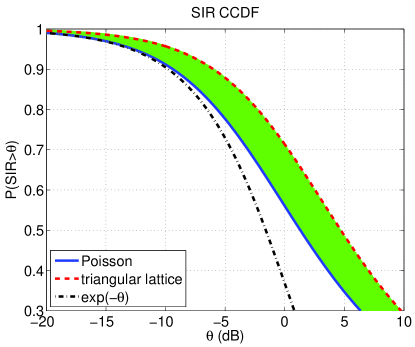
Figure 1: The SIR distributions for the PPP (solid) and the triangular lattice (dashed) for $\alpha=4$ and the lower bound (which is asymptotically tight) $e^{-\theta}$ for the PPP (dash-dotted). The horizontal gap between the SIR distributions of the PPP and the triangular lattice is 3.4 dB for a wide range of $\theta$ values. The shaded band indicates the region in which the SIR distributions for all stationary point process fall that are more regular than the PPP.

An example is shown in Fig. 1, where $\alpha=4$, which results in $\mathsf{MISR}_{\rm PPP}=1$, while for the triangular lattice $\mathsf{MISR}_{\rm tri}=0.457$. Hence the horizontal shift is $\mathsf{MISR}_{\rm PPP}/\mathsf{MISR}_{\rm tri}=3.4$ dB. For Rayleigh fading, we also have the relationship $p_{\rm s}(\theta)=\mathcal{L}_{\mathsf{I{\bar{S}}R}}(\theta)\gtrsim e^{-\theta\,\mathsf{MISR}}$ by Jensen’s inequality, also shown in the figure. Here ’$\gtrsim$’ is a lower bound with asymptotic equality.

In [4], the authors considered coherent and non-coherent joint transmission for the HIP model and derived expressions for the SIR distribution. The diversity gain and the asymptotic pre-constants as $\theta\to 0$ are also derived. In [3], the benefits of BS silencing (inter-cell interference coordination) and re-transmissions (intra-cell diversity) in Poisson networks with Rayleigh fading are studied. For $\theta\to 0$, it is shown that $p_{\rm s}(\theta)\sim 1-a_{k}\theta$ when the $k-1$ strongest interfering BSs are silenced, while $p_{\rm s}(\theta)\sim 1-b_{m}\theta^{m}$ for intra-cell diversity with $m$ transmissions. For $\theta\to\infty$, $p_{\rm s}(\theta)\sim A_{k}\theta^{-\delta}$ and $p_{\rm s}(\theta)\sim B_{m}\theta^{-\delta}$ for BS silencing and retransmissions, respectively. The constants $a_{k}$, $b_{m}$, $A_{k}$, and $B_{m}$ are also determined. Lastly, [8, Thm. 2] gives an expression for the limit $\lim_{\theta\to\infty}\theta^{\delta}p_{\rm s}(\theta)$ for the PPP and the Ginibre point process (GPP) with Rayleigh fading. For the GPP, it consists of a double integral with an infinite product.

In [9], the authors consider a Poisson model for the BSs and define a new point process termed signal-to-total-interference-and-noise ratio (STINR) process. They obtain the moment measures of the new process and use them to express the probability that the user is covered by $k$ BSs. In our work, we consider a different map of the original point process based on relative distances, which results in simplified moment measures for the PPP and permits generalizations to other point process models for the base stations.

I-D Contributions

This paper makes the following contributions:

• We define the relative distance process (RDP), which is the relevant point process for cellular networks with nearest-BS association, and derive some of its pertinent properties, in particular the probability generating functional (PGFL).

• We introduce the generalized MISR, defined as $\mathsf{MISR}_{n}\triangleq(\mathbb{E}(\mathsf{I{\bar{S}}R}^{n}))^{1/n}$, which is applicable to general fading models, and give an explicit expression and tight bounds for the PPP.

• We provide some evidence why the gain $G_{0}$ is insensitive to the path loss exponent $\alpha$ and the fading statistics.

• We show that for all stationary point process models and any type of fading, the tail of the SIR distribution always scales as $\theta^{-\delta}$, i.e., we have $p_{\rm s}(\theta)\sim c\theta^{-\delta}$, $\theta\to\infty$, where the constant $c$ captures the effects of the network geometry and fading. The asymptotic gain follows as

  $$G_{\infty}=\left(\frac{c}{c_{\rm PPP}}\right)^{1/\delta},$$ (8)

  and we have

  $$p_{\rm s}(\theta)\sim p_{\rm s,PPP}(\theta/G_{\infty}),\quad\theta\to\infty.$$

• We introduce the expected fading-to-interference ratio (EFIR) and show that the constant $c$ is related to the EFIR by $c=\mathsf{EFIR}^{\delta}$. Consequently, $G_{\infty}$ is given by the ratio of the EFIR of the general point process under consideration and the EFIR of the PPP.

II System Model

The base station locations are modeled as a simple stationary point process $\Phi\subset\mathbb{R}^{2}$. Without loss of generality, we assume that the typical user is located at the origin $o$. The path loss between the typical user and a BS at $x\in\Phi$ is given by $\ell(x)=\|x\|^{-\alpha}$, $\alpha>2$. Let $\bar{F}_{h}$ denote the ccdf of the iid fading random variables, which are assumed to have mean $1$.

We assume nearest-BS association, wherein a user is served by the closest BS. Let $x_{0}$ denote the closest BS to the typical user at the origin and define $R\triangleq\|x_{0}\|$ and $\Phi^{!}=\Phi\setminus\{x_{0}\}$. With the nearest-BS association rule, the downlink SIR (1) of the typical user can be expressed as

$$\mathsf{SIR}=\frac{hR^{-\alpha}}{\sum_{x\in\Phi^{!}}h_{x}\ell(x)}.$$ (9)

Further notation: $b(o,r)$ denotes the open disk of radius $r$ at $o$, and $b(o,r)^{\rm c}\triangleq\mathbb{R}^{2}\setminus b(o,r)$ is its complement.

III The Relative Distance Process

In this section, we introduce a new point process that is a transformation of the original point process $\Phi$ and helps in the analysis of the interference-to-signal ratio.

III-A Definition

From (1), the MISR is defined as

$$\mathsf{MISR}\triangleq\mathbb{E}\left(\frac{\sum_{x\in\Phi^{!}}h_{x}\ell(x)}{\ell(x_{0})}\right)=\mathbb{E}_{\Phi}\left(\frac{\sum_{x\in\Phi^{!}}\ell(x)}{\ell(x_{0})}\right).$$ (10)

The first expectation is taken over $\Phi$ and $h$, while the second one is only over $\Phi$ since $\mathbb{E}(h)=1$. Since $\ell(x)$ only depends on $\|x\|$, it is apparent that the MISR is determined by the relative distances of the interfering and serving BSs. Accordingly, we introduce a new point process on the unit interval $(0,1)$ that captures only these relative distances.

Definition 2 (Relative distance process (RDP)).

For a simple stationary point process $\Phi$, let $x_{0}=\operatorname{arg~{}min}\{x\in\Phi\colon\|x\|\}$. The relative distance process (RDP) is defined as

$$\mathcal{R}\triangleq\{x\in\Phi\setminus\{x_{0}\}\colon\|x_{0}\|/\|x\|\}\subset(0,1).$$

Using the RDP, the $\mathsf{I{\bar{S}}R}$ can be expressed as

$$\mathsf{I{\bar{S}}R}=\sum_{y\in\mathcal{R}}h_{y}y^{\alpha},$$

and, since $\mathbb{E}(h_{y})=1$, the MISR is

$$\mathsf{MISR} =\mathbb{E}\sum_{y\in\mathcal{R}}y^{\alpha}=\int_{0}^{1}r^{\alpha}\Lambda({\rm d}r).$$

For the stationary PPP, the cdfs of the elements $\nu_{k}=\|x_{0}\|/\|x_{k}\|$ of $\mathcal{R}$ are $F_{\nu_{k}}(x)=1-(1-x^{2})^{k}$, $x\in[0,1]$, as given in [6]. Summing the densities ${\rm d}F_{\nu_{k}}(x)/{\rm d}x$ over $k\in\mathbb{N}$ yields the intensity measure $\Lambda({\rm d}r)=2r^{-3}{\rm d}r$. It follows that the mean measure $\Lambda([r,1))\triangleq\mathbb{E}\mathcal{R}([r,1))=r^{-2}-1$, $0<r<1$. The fact that the mean measure diverges near $0$ is consistent with the fact that $\mathcal{R}$ is not locally finite on intervals $[0,\epsilon)$.

Generally, since the MISR only depends on the relative distances, the gain $G_{0}$ does not depend on the base station density.

III-B RDP of the PPP

The success probability for Rayleigh fading is given by the Laplace transform of the $\mathsf{I{\bar{S}}R}$:

$$p_{\rm s}(\theta)=\mathbb{E}e^{-\theta\,\mathsf{I{\bar{S}}R}}=\mathbb{E}\prod_{y\in\mathcal{R}}e^{-\theta h_{y}y^{\alpha}}=\mathbb{E}\prod_{y\in\mathcal{R}}\frac{1}{1+\theta y^{\alpha}}$$ (11)

This RDP-based formulation has the advantage that it circumvents the usual two-step procedure, where first the conditional success probability given the distance to the serving base station $R$ is calculated and then an expectation with respect to $R$ is taken.

Since (11) has the form of a PGFL, we first calculate the PGFL of the RDP generated by a PPP.

Lemma 1.

When $\Phi$ is a PPP, the probability generating functional of the RDP is given by

$$G_{\mathcal{R}}[f]\triangleq\mathbb{E}\prod_{x\in\mathcal{R}}f(x)= \frac{1}{1+2\int_{0}^{1}(1-f(x))x^{-3}{\rm d}x},$$ (12)

for functions $f\colon[0,1]\mapsto[0,1]$ such that the integral in the denominator of (12) is finite.

Proof:

The PGFL $G_{\mathcal{R}}[f]$ can be calculated as

$$G_{\mathcal{R}}[f] =\mathbb{E}\left[\prod_{x\in\mathcal{R}}f(x)\right]$$

$$=\mathbb{E}\left[\prod_{x\in\Phi\setminus\{x_{0}\}}f\left(\frac{\|x_{0}\|}{\|x\|}\right)\right]$$

$$\stackrel{{\scriptstyle(a)}}{{=}}\mathbb{E}_{R}\exp\left(-2\pi\lambda\int_{R}^{\infty}a\left(1-f\left(\frac{R}{a}\right)\right){\rm d}a\right)$$

$$\stackrel{{\scriptstyle(b)}}{{=}}\lambda\int\limits_{0}^{\infty}2\pi r\exp\left(-2\pi\lambda\int\limits_{r}^{\infty}a\left(1-f\left(\frac{r}{a}\right)\right){\rm d}a\right)e^{-\lambda\pi r^{2}}{\rm d}r$$

$$=\lambda\int\limits_{0}^{\infty}2\pi r\exp\left(-2\pi r^{2}\lambda\int\limits_{1}^{\infty}y\left(1-f\left(\frac{1}{y}\right)\right){\rm d}y\right)e^{-\lambda\pi r^{2}}{\rm d}r$$

$$=\frac{1}{1+2\int_{1}^{\infty}y\left(1-f(1/y)\right){\rm d}y},$$

where $(a)$ is obtained from the PGFL of the PPP, which, for a general PPP $\Psi$ with intensity measure $\Lambda$, is given by

$$G_{\Psi}[f]\triangleq\mathbb{E}\prod_{x\in\Psi}f(x)=\exp\left(-\int_{\mathbb{R}^{2}}[1-f(x)]\Lambda({\rm d}x)\right).$$ (13)

Writing the PGFL in polar form and conditioning on the distance to the nearest neighbor $R=\|x_{0}\|$ yields $(a)$. In $(b)$, we de-condition on $R$ using the the nearest-neighbor distribution of the PPP. Using the substitution $y^{-1}\to x$, we obtain the final result. ∎

When $f(x)=1/(1+\theta x^{\alpha})$ (see (11)), we retrieve the result in (3) for Poisson cellular networks with Rayleigh fading.

It may be suspected that the RDP of a PPP is itself a (non-stationary) PPP on $[0,1]$. It is easily seen that this is not the case. Let $\Psi$ be a PPP on $[0,1$] with the same intensity function as $\mathcal{R}$, i.e., $\Lambda({\rm d}r)=2r^{-3}{\rm d}r$. If $\mathcal{R}$ was a PPP, the success probability for Rayleigh fading would follow from the PGFL of $\Psi$ (specializing (13) to a PPP on $[0,1]$) as

$$G_{\Psi}[f]=\exp\left(-\int_{0}^{1}[1-f(r)]2r^{-3}{\rm d}r\right),$$

and, in turn, the success probability would be given by

$$\tilde{p}_{\rm s}(\theta)=\exp\left(-\int_{0}^{1}\frac{\theta r^{\alpha}}{1+\theta r^{\alpha}}2r^{-3}{\rm d}r\right)$$ (14)

instead of (3).

However, assuming $\mathcal{R}$ to be Poisson yields an approximation of the success probability, with asymptotic equality as $\theta\to 0$. The “Poisson approximation” (14) is related to the actual value (3) as

$$\tilde{p}_{\rm s}(\theta)=\exp\left(1-\frac{1}{p_{\rm s}(\theta)}\right),$$

This holds due to the identity

$$\frac{\delta\theta\,_{2}F_{1}\left(1,1-\delta;2-\delta;-\theta\right)}{1-\delta}\equiv\,_{2}F_{1}(1,-\delta;1-\delta;-\theta)-1.$$

Rewriting and expanding, we have

$$\tilde{p}_{\rm s}(\theta)=\frac{1}{\exp(1/p_{\rm s}(\theta)-1)}=\frac{1}{\frac{1}{p_{\rm s}(\theta)}+\frac{1}{2}\left(\frac{1}{p_{\rm s}(\theta)}-1\right)^{2}+\ldots}.$$

Hence, only considering the dominant first term in the denominator as $\theta\to 0$, we obtain $\tilde{p}_{\rm s}(\theta)\sim p_{\rm s}(\theta)$, $\theta\to 0$.

The fact that $\tilde{p}_{\rm s}(\theta)<p_{\rm s}(\theta)$ for $\theta>0$ is an indication that the higher moment densities of the RDP are larger than those of the PPP. This is indeed the case, as the following calculation of the moment densities shows.

Lemma 2.

When $\Phi$ is a PPP, the moment densities of the RDP are given by

$$\rho^{(n)}(t_{1},t_{2},\ldots,t_{n})=n!\,2^{n}\prod_{i=1}^{n}t_{i}^{-3}.$$ (15)

Proof:

First we obtain the factorial moment measures. We use the simplified notation

$$\alpha^{(n)}(t_{1},t_{2},\ldots,t_{n})\equiv\alpha^{(n)}((t_{1},1)\times(t_{2},1)\times\ldots\times(t_{n},1)),\quad 0<t_{i}\leq 1.$$

The factorial moment measures are defined as

$$\alpha^{(n)}(t_{1},t_{2},\ldots,t_{n})=\mathbb{E}\sum_{x_{1},x_{2},\ldots,x_{n}\in\mathcal{R}}^{\neq}\mathbf{1}_{(t_{1},1)}(x_{1})\mathbf{1}_{(t_{2},1)}(x_{2})\cdots\mathbf{1}_{(t_{n},1)}(x_{n}),$$

where $\sum^{\neq}$ indicates that the sum is taken over $n$-tuples of distinct points. The moment measures are related to the PGFL as [10, p. 116]

$$\alpha^{(n)}(t_{1},t_{2},\ldots,t_{n})\equiv(-1)^{n}\frac{\partial}{\partial s_{1}}\ldots\frac{\partial}{\partial s_{n}}G_{\mathcal{R}}[1-s_{1}\mathbf{1}_{(t_{1},1)}-s_{2}\mathbf{1}_{(t_{2},1)}-\ldots-\mathbf{1}_{(t_{n},1)}]$$ (16)

evaluated at $s_{1}=s_{2}=\ldots=s_{n}=0$. Using Lemma 1 we obtain

$$G_{\mathcal{R}}[1-s_{1}\mathbf{1}_{(t_{1},1)}-s_{2}\mathbf{1}_{(t_{2},1)}-\ldots-s_{n}\mathbf{1}_{(t_{n},1)}]=\\ \frac{1}{1+\sum_{i=1}^{n}s_{i}(t_{i}^{-2}-1)}.$$

Differentiating with respect to $s_{i}$ and setting $s_{1}=s_{2}=\cdots=s_{n}=0$, we have

$$\alpha^{(n)}(t_{1},t_{2},\ldots,t_{n})=n!\prod_{i=1}^{n}\left(\frac{1}{t_{i}^{2}}-1\right).$$ (17)

The moment densities follow from differentiation, noting that $t_{i}$ denotes the start of the interval, which causes a sign change since increasing $t_{i}$ decreases the measure. ∎

So the product densities are a factor $n!$ larger than they would be if $\mathcal{R}$ was a PPP. This implies, interestingly, that the pair correlation function [11, Def. 6.6] of the RDP of the PPP is $g(x,y)=2$, $\forall x,y\in(0,1)$.

The moment densities of the RDP provide an alternative way to obtain the success probability for the PPP:

$$p_{\rm s}(\theta) =\mathbb{E}\prod_{y\in\mathcal{R}}\frac{1}{1+\theta y^{\alpha}}=\mathbb{E}\prod_{y\in\mathcal{R}}\left(1-\frac{1}{1+\theta^{-1}y^{-\alpha}}\right)$$

$$=1-\sum_{y\in\mathcal{R}}\nu(\theta,y)+\frac{1}{2!}\mathbb{E}\sum^{\neq}_{y_{1},y_{2}\in\mathcal{R}}\nu(\theta,y_{1})\nu(\theta,y_{2})+\ldots+\frac{(-1)^{n}}{n!}\mathbb{E}\sum^{\neq}_{y_{1},\ldots,y_{n}\in\mathcal{R}}\prod_{i=1}^{n}\nu(\theta,y_{i})+\ldots,$$

where $\nu(\theta,y)=\frac{1}{1+\theta^{-1}y^{-\alpha}}$. From the definition of the moment densities, we have

$$p_{\rm s}(\theta) =\sum_{n=0}^{\infty}\frac{(-1)^{n}}{n!}\mathbb{E}\sum^{\neq}_{y_{1},\ldots,y_{n}\in\mathcal{R}}\prod_{i=1}^{n}\nu(\theta,y_{i})$$

$$=\sum_{n=0}^{\infty}\frac{(-1)^{n}}{n!}\int_{[0,1]^{n}}\left(\prod_{i=1}^{n}\nu(\theta,t_{i})\right)\rho^{(n)}(t_{1},t_{2},\ldots,t_{n}){\rm d}t_{1}\ldots{\rm d}t_{n}$$ (18)

Using Lemma 2, we have

$$p_{\rm s}(\theta) =\sum_{n=0}^{\infty}{2^{n}(-1)^{n}}\left(\int_{[0,1]}\nu(\theta,t)t^{-3}{\rm d}t\right)^{n},$$

$$=\sum_{n=0}^{\infty}{\theta^{n}(-1)^{n}}\left(\frac{\delta\,_{2}F_{1}\left(1,1-\delta;2-\delta;-\theta\right)}{1-\delta}\right)^{n}$$

$$=\sum_{n=0}^{\infty}{\theta^{n}(-1)^{n}}\left(\,{}_{2}F_{1}(1,-\delta;1-\delta;-\theta)-1\right)^{n}$$

$$=\frac{1}{\,{}_{2}F_{1}(1,-\delta;1-\delta;-\theta)},$$

which equals the success probability given in (3).

III-C RDP of a stationary point process

We now characterize the PGFL of the RDP generated by a stationary point process. Let $f(R,\Phi^{!})$ be a positive function of the distance $R=\|x_{0}\|$ and the point process $\Phi^{!}=\Phi\setminus\{x_{0}\}$. The average $\mathbb{E}[f(R,\Phi^{!})]$ can in principle be evaluated using the joint distribution of $R$ and $\Phi$, which is, however, known only for a few point processes. Thus we introduce an alternative representation of $f(R,\Phi^{!})$ that is easier to work with.

The indicator variable $\mathbf{1}(\Phi(b(o,\|x\|))=0)$, $x\in\Phi$, equals one only when $x=x_{0}$. Hence it follows that

$$f(R,\Phi^{!})\equiv\sum_{x\in\Phi}f(\|x\|,\Phi\setminus\{x\})\mathbf{1}(\Phi(b(o,\|x\|))=0).$$ (19)

This representation of $f(R,\Phi^{!})$ permits the computation of the expectation of $f(R,\Phi^{!})$ using the Campbell-Mecke theorem [11, Thm. 8.2]. We use the above idea in the next lemma to obtain the PGFL of a general RDP.

Lemma 3.

The PGFL of the RDP generated by a stationary point process $\Phi$ is given by

$$G_{\cal R}[f]=\lambda\int_{\mathbb{R}^{2}}\mathcal{G}^{!}_{o}\left[f\left(\frac{\|x\|}{\|\cdot+x\|}\right)\mathbf{1}(\cdot+x\in b(o,\|x\|)^{\rm c})\right]{\rm d}x,$$ (20)

where $\mathcal{G}^{!}_{o}$ is the PGFL of the point process $\Phi$ with respect to the reduced Palm measure.

Proof:

Using the representation in (19), we obtain

$$G_{\mathcal{R}}[f] =\mathbb{E}\sum_{x\in\Phi}\prod_{y\in\Phi\setminus\{x\}}f\left(\frac{\|x\|}{\|y\|}\right)\mathbf{1}(\Phi(b(o,\|x\|))=0)$$

$$\stackrel{{\scriptstyle{\rm(a)}}}{{=}}\lambda\int_{\mathbb{R}^{2}}\mathbb{E}_{o}^{!}\prod_{y\in\Phi}f\left(\frac{\|x\|}{\|y+x\|}\right)\mathbf{1}(\Phi(b(-x,\|x\|))=0){\rm d}x$$

$$=\lambda\int_{\mathbb{R}^{2}}\mathbb{E}_{o}^{!}\prod_{y\in\Phi}f\left(\frac{\|x\|}{\|y+x\|}\right)\mathbf{1}(y\in b(-x,\|x\|)^{\rm c}){\rm d}x$$

$$=\lambda\int_{\mathbb{R}^{2}}\mathcal{G}_{o}^{!}\left[f\left(\frac{\|x\|}{\|\cdot+x\|}\right)\mathbf{1}(\cdot+x\in b(o,\|x\|)^{\rm c})\right]{\rm d}x,$$

where $(a)$ follows from the Campbell-Mecke theorem. ∎

If $\Phi$ is also rotationally invariant (i.e., motion-invariant), the reduced Palm measure is also rotationally invariant and hence

$$G_{\cal R}[f]=\lambda 2\pi\int\limits_{0}^{\infty}r\mathcal{G}_{o}^{!}\left[f\left(\frac{r}{\|\cdot+r\|}\right)\mathbf{1}(\cdot+r\in b(o,r)^{\rm c})\right]{\rm d}r,$$ (21)

where $r$ in any vector addition should be interpreted as $(r,0)$.

Remark. Taking $\Phi$ to be a PPP, (21) reduces to (12) since

$$G_{\mathcal{R}}[f] =2\pi\lambda\int_{0}^{\infty}r\exp\Bigg{(}-\lambda\int_{\mathbb{R}^{2}}\bigg{[}1-f\left(\frac{r}{\|x+(r,0)\|}\right)\mathbf{1}(x+(r,0)\in b(0,r)^{\rm c})\bigg{]}{\rm d}x\Bigg{)}{\rm d}r$$

$$=2\pi\lambda\int\limits_{0}^{\infty}r\exp\bigg{(}-\lambda\pi r^{2}-\lambda\int\limits_{b(o,r)^{c}}\left[1-f\left(\frac{r}{\|x\|}\right)\right]{\rm d}x\bigg{)}{\rm d}r$$

$$=2\pi\lambda\int_{0}^{\infty}r\exp\left(-\lambda\pi r^{2}-2\pi\lambda\int_{r}^{\infty}y[1-f(r/y)]{\rm d}y\right){\rm d}r.$$

The last expression equals the second-to-last line in the proof of Lemma 1.

Similar to the case of PPP, we now obtain the moment measures of the RDP of a general stationary point process.

Lemma 4.

The factorial moment measures of the RDP $\mathcal{R}$ generated by a stationary point process $\Phi$ are

$$\alpha^{(n)}(t_{1},t_{2},\ldots,t_{n})=\int\limits_{\mathbb{R}^{n+1}}\prod_{i=1}^{n}f(y_{0},y_{i},t_{i})\mathbb{E}^{!}_{y_{0},y_{1},\ldots,y_{n}}[g(\Phi,y_{0})]\rho^{(n+1)}_{\Phi}(y_{0},y_{1},\ldots,y_{n}){\rm d}y_{0}\ldots{\rm d}y_{n},$$ (22)

where $g(\Psi,x)=\prod_{y\in\Psi}\mathbf{1}(\|y\|\geq\|x\|)$ and $f(x,y,t)=\mathbf{1}_{(t,1)}\left(\frac{\|x\|}{\|y\|}\right)$. The product densities are

$$\rho^{(n)}_{\mathcal{R}}(t_{1},t_{2},\ldots,t_{n})=n!\,2^{n}\left(\prod_{i=1}^{n}t_{i}^{-3}\right)\beta_{n}(t_{1},\ldots,t_{n}),$$ (23)

where

$$\beta_{n}(t_{1},\ldots,t_{n})\triangleq \frac{1}{n!2^{n}}\int\limits_{\mathbb{R}^{2}}\|y_{0}\|^{2n}\int\limits_{[0,2\pi]^{n}}\mathbb{E}^{!}_{y_{0},\left(\frac{\|y_{0}\|}{t_{1}},\varphi_{1}\right),\ldots,\left(\frac{\|y_{0}\|}{t_{n}},\varphi_{n}\right)}[g(\Phi,y_{0})]\cdot$$

$$\;\rho^{(n+1)}_{\Phi}\left(y_{0},\Big{(}\frac{\|y_{0}\|}{t_{1}},\varphi_{1}\Big{)},\ldots,\Big{(}\frac{\|y_{0}\|}{t_{n}},\varphi_{n}\Big{)}\right){\rm d}\varphi_{1}\ldots{\rm d}\varphi_{n}{\rm d}y_{0}.$$ (24)

Proof:

As before, we use the relationship (16). While the result can be obtained from the PGFL in Lemma 1, it is easier to begin with the definition of the PGFL. We have

$$G_{\mathcal{R}}[f] =\mathbb{E}\sum_{x\in\Phi}\prod_{y\in\Phi\setminus\{x\}}f\left(\frac{\|x\|}{\|y\|}\right)\mathbf{1}(\|y\|\geq\|x\|)$$

$$=\mathbb{E}\sum_{x\in\Phi}g(\Phi\setminus\{x\},x)\prod_{y\in\Phi\setminus\{x\}}f\left(\frac{\|x\|}{\|y\|}\right).$$

We are interested in the derivative of the PGFL with the function $f(z)=1-\sum_{i=1}^{n}s_{i}\mathbf{1}_{(t_{i},1)}(z)$. So we have

$$\alpha^{(n)}(t_{1},t_{2},\ldots,t_{n})=(-1)^{n}\frac{\partial}{\partial s_{1}}\ldots\frac{\partial}{\partial s_{n}}\mathbb{E}\sum_{x\in\Phi}g(\Phi\setminus\{x\},x)\prod_{y\in\Phi\setminus\{x\}}\left(1-\sum_{i=1}^{n}s_{i}\mathbf{1}_{(t_{i},1)}\left(\frac{\|x\|}{\|y\|}\right)\right)$$

evaluated at $s_{1}=s_{2}=\ldots=s_{n}=0$. Expanding the inner product over the summation we obtain an infinite polynomial in the powers of $s_{1},\ldots,s_{n}$ and their products. We observe that the only term that contributes to the derivative in a non-zero manner is the $s_{1}s_{2}\cdots s_{n}$ term. Its coefficient equals

$$T=(-1)^{n}\mathbb{E}\bigg{(}\sum_{x\in\Phi}g(\Phi\setminus\{x\},x)\sum_{y_{1},\ldots y_{n}\in\Phi\setminus\{x\}}^{\neq}f(x,y_{1},t_{1})\ldots f(x,y_{n},t_{n})\bigg{)}.$$

Combining the summations,

$$T=(-1)^{n}\mathbb{E}\bigg{(}\sum_{y_{0},y_{1},\ldots y_{n}\in\Phi}^{\neq}f(y_{0},y_{1},t_{1})\cdot\ldots\cdot f(y_{0},y_{n},t_{n})g(\Phi\setminus\{y_{0}\},y_{0})\bigg{)}.$$

Since $f(y_{0},y_{i},t_{i})\neq 1$ implies $\|y_{i}\|\geq\|y_{0}\|$,

$$T=(-1)^{n}\mathbb{E}\bigg{(}\sum_{y_{0},y_{1},\ldots y_{n}\in\Phi}^{\neq}f(y_{0},y_{1},t_{1})\cdot\ldots\cdot f(y_{0},y_{n},t_{n})g(\Phi\setminus\{y_{0},y_{1},\ldots,y_{n}\},y_{0})\bigg{)},$$

and, using [12, Thm. 1],

$$T=(-1)^{n}\int_{\mathbb{R}^{n+1}}\prod_{i=1}^{n}f(y_{0},y_{i},t_{i})\mathbb{E}^{!}_{y_{0},y_{1},\ldots,y_{n}}[g(\Phi,y_{0})]\cdot\\ \rho^{(n+1)}_{\Phi}(y_{0},y_{1},\ldots,y_{n}){\rm d}y_{0}\ldots{\rm d}y_{n},$$ (25)

and the result (22) follows. For the product densities, we convert the variables $x_{i}$ into polar coordinates $(r_{i},\varphi_{i})$, which yields

$$\alpha^{n}(t_{1},t_{2},\ldots,t_{n}) =\int\limits_{\mathbb{R}^{2}}\int\limits_{\|y_{0}\|}^{\|y_{0}\|/t_{1}}\!\!r_{1}\cdots\!\!\int\limits_{\|y_{0}\|}^{\|y_{0}\|/t_{n}}r_{n}\!\!\int\limits_{[0,2\pi]^{n}}\!\!\mathbb{E}^{!}_{y_{0},(r_{1},\varphi_{1}),\ldots,(r_{n},\varphi_{n})}[g(\Phi,y_{0})]$$

$$\qquad\cdot\rho^{(n+1)}(y_{0},(r_{1},\varphi_{1}),..,(r_{n},\varphi_{n})){\rm d}\varphi_{1}\ldots{\rm d}\varphi_{n}{\rm d}r_{1}\ldots{\rm d}r_{n}{\rm d}y_{0}.$$

Then differentiating using the Leibniz rule with respect to $t_{1},\ldots,t_{n}$, we obtain

$$\rho^{(n)}_{\mathcal{R}}(t_{1},t_{2},\ldots,t_{n})=\left(\prod_{i=1}^{n}t_{i}^{-3}\right)\int\limits_{\mathbb{R}^{2}}\|y_{0}\|^{2n}\int\limits_{[0,2\pi]^{n}}\mathbb{E}^{!}_{y_{0},\left(\frac{\|y_{0}\|}{t_{1}},\varphi_{1}\right),\ldots,\left(\frac{\|y_{0}\|}{t_{n}},\varphi_{n}\right)}[g(\Phi,y_{0})]\cdot\\ \rho^{(n+1)}_{\Phi}\left(y_{0},\left(\frac{\|y_{0}\|}{t_{1}},\varphi_{1}\right),\ldots,\left(\frac{\|y_{0}\|}{t_{n}},\varphi_{n}\right)\right){\rm d}\varphi_{1}\ldots{\rm d}\varphi_{n}{\rm d}y_{0},$$

which equals (23). ∎

As in (18), the moment densities of the RDP generated by a stationary point process can be used to compute its corresponding success probability.

IV The Mean Interference-to-Signal Ratio (MISR) and the Gain at $0$

In this section, we introduce and analyze the MISR, including its generalized version, and apply it to derive a simple asymptotic expression of the SIR distribution near $0$ using the gain $G_{0}$. We also give some insight why $G_{0}$ barely depends on the path loss exponent $\alpha$ and the fading statistics.

IV-A The MISR for general point processes

The first result gives an expression for the MISR for a general point process.

Theorem 1.

The MISR of a motion-invariant point process $\Phi$ is given by

$$\mathsf{MISR}=2\int_{0}^{1}t^{\alpha-3}\beta_{1}(t){\rm d}t,$$

where $\beta_{1}(t)$ is given in (24) in Lemma 4.

Proof:

Using the RDP, the MISR can be expressed as

$$\mathsf{MISR} =\mathbb{E}\sum_{y\in\mathcal{R}}y^{\alpha}$$

$$=\int_{0}^{1}t^{\alpha}\rho^{(1)}_{\mathcal{R}}(t){\rm d}t.$$

$$\stackrel{{\scriptstyle(a)}}{{=}}2\int_{0}^{1}t^{\alpha}t^{-3}\beta_{1}(t){\rm d}t,$$

where $(a)$ follows from Lemma 4. ∎

When $\Phi$ is a PPP, from Slivnyak’s theorem and the fact that $\rho^{(2)}=\lambda^{2}$, we have $\beta_{1}(t)=1$ and hence $\mathsf{MISR}=2/(\alpha-2)$.

IV-B The Generalized MISR

Definition 3 (Generalized MISR).

The generalized MISR with parameter $n$ is defined as

$$\mathsf{MISR}_{n}\triangleq(\mathbb{E}(\mathsf{I{\bar{S}}R}^{n}))^{1/n}.$$

If there is a danger of confusion, we call $\mathsf{MISR}\equiv\mathsf{MISR}_{1}$ the standard MISR.

The generalized MISR can be obtained by taking the corresponding derivative of the Laplace transform $\mathbb{E}(e^{-s\,\mathsf{I{\bar{S}}R}})$ at $s=0$. In case of the PPP with Rayleigh fading, the Laplace transform is known and equals the success probability (3), thus

$$\mathsf{MISR}_{n}^{n}=\mathbb{E}(\mathsf{I{\bar{S}}R}^{n})=(-1)^{n}\frac{{\rm d}}{{\rm d}\theta^{n}}p_{\rm s}(\theta)\big{|}_{\theta=0}.$$ (26)

For general fading, the Laplace transform is not known, but we can still calculate the derivative at $s=0$, as the following result for the PPP with general fading shows.

Theorem 2 (Generalized MISR and lower bound for PPP).

For a Poisson cellular network with arbitrary fading,

$$\mathbb{E}(\mathsf{I{\bar{S}}R}^{n})=\sum_{k=1}^{n}k!B_{n,k}\left(\frac{\delta}{1-\delta},\ldots,\frac{\delta\mathbb{E}(h^{n-k+1})}{n-k+1-\delta}\right),$$ (27)

where $B_{n,k}$ are the (incomplete) Bell polynomials. For $n>1$, the generalized MISR is lower bounded as

$$\mathsf{MISR}_{n}\geq\left[\left(\frac{\delta}{1-\delta}\right)^{n}n!+\frac{\delta\mathbb{E}(h^{n})}{n-\delta}\right]^{1/n}.$$ (28)

For $n=2$, equality holds, and for $\delta\to 0$ and $\delta\to 1$, the lower bound is asymptotically tight.

Proof:

We begin with the the Laplace transform of the $\mathsf{I{\bar{S}}R}$, given by

$$\mathbb{E}(e^{-s\,\mathsf{I{\bar{S}}R}}) =\mathbb{E}\prod_{y\in\mathcal{R}}\mathcal{L}_{h}(sy^{\alpha})$$

$$\stackrel{{\scriptstyle(a)}}{{=}}\frac{1}{1+2\int_{1}^{\infty}y\left(1-\mathcal{L}_{h}\left(\frac{s}{y^{\alpha}}\right)\right){\rm d}y}.$$

where $(a)$ follows from Lemma 1. Let $f(s)=1/(1+s)$ and $g(s)=2\int_{1}^{\infty}y\left(1-\mathcal{L}_{h}\left(\frac{s}{y^{\alpha}}\right)\right){\rm d}y$. Then $\mathbb{E}(e^{-s\,\mathsf{I{\bar{S}}R}})=f(g(s))$. We are interested in the $m$-derivative of $\mathbb{E}(e^{-s\,\mathsf{I{\bar{S}}R}})$ with respect to $s$ at $s=0$, which can be computed using Faà di Bruno’s formula [13] as

$$\frac{{\rm d}}{{\rm d}s}f(g(s))|_{s=0}=\\ \sum_{k=1}^{n}f^{(k)}(g(0))B_{n,k}(g^{\prime}(0),g^{\prime\prime}(0),...,g^{(n-k+1)}(0)),$$

where $B_{n,k}$ are the (incomplete) Bell polynomials. We have $g(0)=0$,

$$f^{(k)}(s)=(-1)^{k}\frac{k!}{(1+s)^{k+1}},$$

and

$$g^{(k)}(s)=-2\int_{1}^{\infty}y^{1-k\alpha}\mathcal{L}_{h}^{(k)}(sy^{-\alpha}){\rm d}y,$$

which, when evaluated at $s=0$, equals

$$g^{(k)}(0)=\frac{2(-1)^{k+1}\mathbb{E}(h^{k})}{k\alpha-2}.$$

Combining everything, we have

$$\mathbb{E}(\mathsf{I{\bar{S}}R}^{n}) =(-1)^{n}\frac{{\rm d}^{n}}{{\rm d}s^{n}}\mathbb{E}(e^{-s\,\mathsf{I{\bar{S}}R}})\big{|}_{s=0}$$

$$=(-1)^{n}\sum_{k=1}^{n}(-1)^{k}k!B_{n,k}\left(\frac{2}{\alpha-2},\ldots,\frac{2(-1)^{n-k}\mathbb{E}(h^{n-k+1})}{(n-k+1)\alpha-2}\right).$$ (29)

From the definition of Bell polynomials it follows that all the terms are positive, hence the result (27) follows from $\delta=2/\alpha$. The lower bound is obtained by only considering the terms $k=1$ and $k=m$ in the sum (29). The bound becomes tight as $\delta\to 0$ and as $\delta\to 1$ since the term $k=1$ dominates the sum (29) as $\delta\to 1$ since it is the only term with a denominator $(1-\delta)^{n}$, while the term $k=n$ dominates as $\delta\to 0$ since it is the only one with a numerator $\Theta(\delta)$. ∎

Hence we have two simpler asymptotically tight bounds for the generalized MISR:

$$\mathsf{MISR}_{n} \gtrsim\left(\frac{\delta}{n}\mathbb{E}(h^{n})\right)^{1/n},\quad\delta\to 0$$ (30)

$$\mathsf{MISR}_{n} \gtrsim\frac{\delta(n!)^{1/n}}{1-\delta}=\mathsf{MISR}_{1}(n!)^{1/n},\quad\delta\to 1.$$ (31)

For Rayleigh fading, (30) yields $\mathsf{MISR}_{n}\sim(\delta\Gamma(n))^{1/n}$, $\delta\to 0$.

Fig. 2 shows $\mathsf{MISR}_{n}$ for Rayleigh fading as a function of the path loss exponent. As can be observed, the term $\mathsf{MISR}_{1}(n!)^{1/n}$ is dominant for $\alpha\leq 4$ even if the fading is severe (Rayleigh fading). For less severe fading, the term with $\mathbb{E}(h^{n})$ is less relevant; it only becomes dominant for unrealistically high path loss exponents ($\delta\ll 1$).

The second moment of the $\mathsf{I{\bar{S}}R}$ follows from (27) as

$$\mathbb{E}(\mathsf{I{\bar{S}}R}^{2})=2\,\mathsf{MISR}_{1}^{2}+\frac{\delta\mathbb{E}(h^{2})}{2-\delta},$$

and the third moment is

$$\mathbb{E}(\mathsf{I{\bar{S}}R}^{3})=6\,\mathsf{MISR}_{1}^{3}+\frac{6\delta^{2}\mathbb{E}(h^{2})}{(1-\delta)(2-\delta)}+\frac{\delta\mathbb{E}(h^{3})}{3-\delta}.$$

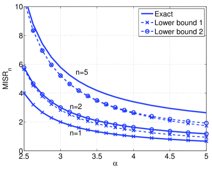
Figure 2: $\mathsf{MISR}_{n}$ for $n\in\{1,2,5\}$ for the PPP with Rayleigh fading as a function of the path loss exponent $\alpha$. “Lower bound 1” is the simple bound in (31), which holds irrespective of the fading and is asymptotically tight as $\alpha\downarrow 2$, and “Lower bound 2” is the bound in (28), which is valid for $n\geq 2$ and is exact for $n=2$. For $\alpha\leq 4$, the two bounds are essentially identical.

Remarks.

• Setting $\mathbb{E}(h^{k})=1$ for all $k$ retrieves the result in [3, Prop. 3] on the pre-constant for $m$ transmissions in a Poisson networks over Rayleigh fading.

• An alternative way to derive the lower bound is as follows. Letting $u_{y}\triangleq h_{y}y^{\alpha}$ for $y\in\mathcal{R}$, we expand $\mathsf{I{\bar{S}}R}^{n}$ as

  $$\mathsf{I{\bar{S}}R}^{n} =\left(\sum_{y\in\mathcal{R}}u_{y}\right)^{n}$$

  $$=\sum_{y\in\mathcal{R}}u_{y}^{n}+\binom{n}{1}\sum_{y\in\mathcal{R}}\left(u_{y}^{n-1}\sum_{x\in\mathcal{R}\setminus\{y\}}u_{x}\right)+\binom{n}{2}\sum_{y\in\mathcal{R}}\left(u_{y}^{n-2}\sum_{x,z\in\mathcal{R}\setminus\{y\}}u_{x}u_{z}\right)+$$

  $$\;\;\binom{n}{3}\sum_{y\in\mathcal{R}}\left(u_{y}^{k-3}\sum_{v,x,z\in\mathcal{R}\setminus\{y\}}u_{v}u_{x}u_{z}\right)+\underbrace{\ldots}_{n-4\text{ terms}}+\binom{n}{n}\sum_{x_{1},\ldots,x_{n}\in\mathcal{R}}^{\neq}u_{x_{1}}\cdots u_{x_{n}},$$

  where the expression contains $k$ sums. Ignoring all but the first and last terms of the expansion, we obtain

  $$\mathbb{E}(\mathsf{I{\bar{S}}R}^{n}) \geq\mathbb{E}(h^{n})\frac{\delta}{m-\delta}+\int_{[0,1]^{n}}(x_{1}\cdots x_{n})^{\alpha}\rho_{\Phi}^{(n)}(x_{1},\ldots,x_{n}){\rm d}x_{1}\cdots{\rm d}x_{n}$$

  $$=\mathbb{E}(h^{n})\frac{\delta}{n-\delta}+n!\,\mathsf{MISR}_{1}^{n},$$

  which equals the result in (28).

For Nakagami-$m$ fading, $\mathsf{MISR}_{n}$ is decreasing with increasing $m$ since the moments $\mathbb{E}(h^{n})$ are decreasing with $m$. As the lower bound $\mathsf{MISR}_{1}(n!)^{1/n}$ does not depend on the fading, $\mathsf{MISR}_{n}$ approaches a non-trivial limit as $m\to\infty$.

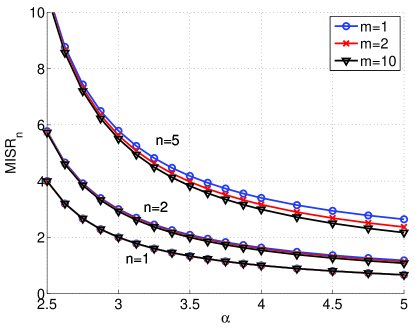
(a) $\mathsf{MISR}_{n}$ as a function of $\alpha$ for $n\in\{1,2,5\}$.

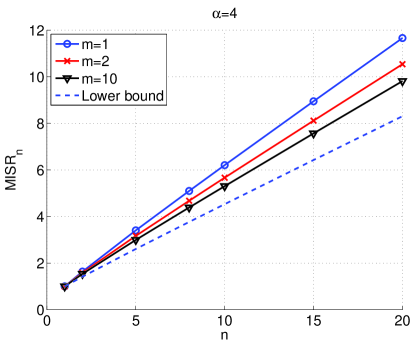
(b) $\mathsf{MISR}_{n}$ as a function of $n$ for $\alpha=4$ and lower bound (31).

Figure 3: Generalized MISR per (27) for the PPP for Nakagami-$m$ fading with $m\in\{1,2,10\}$.

Fig. 3 shows $\mathsf{MISR}_{n}$ as a function of $n$. The increase is almost linear in $n$. Indeed, as $n\to\infty$, $\mathsf{MISR}_{n}$ is proportional to $n$ for the usually encountered path loss exponents, as the following corollary establishes.

Corollary 3.

For the PPP with Rayleigh fading and $\alpha\leq 4$,

$$\mathsf{MISR}_{n}\sim\frac{n}{e}\,\mathsf{MISR}_{1}=\frac{n}{e}\frac{\delta}{1-\delta},\quad n\to\infty.$$

Proof:

For the PPP with Rayleigh fading and $\delta\geq 1/2$, it follows from (27) that

$$\mathsf{MISR}_{n}\sim\left(\frac{\delta}{1-\delta}\right)(n!)^{1/n},\quad n\to\infty,$$

since the dominant term in (27) for large $n$ is the one with $\delta^{n}/(1-\delta)^{n}$, which increases geometrically (or stays constant) with $n$ for $\delta\geq 1/2$. For the factorial term, $\log((n!)^{1/n})\sim\log n-1$, hence we obtain $\mathsf{MISR}_{n}\sim e^{\log n-1}\,\mathsf{MISR}_{1}$. ∎

Remark. Using Stirling’s formula $n!\sim\sqrt{2\pi n}(n/e)^{n}$, this asymptotic result can be sharpened slightly.

IV-C The gain $G_{0}$ for general fading

Equipped with the results from Theorem 2, we can now discuss the gain $G_{0}$ for general fading. If $F_{h}(x)\sim c_{m}x^{m}$, $x\to 0$, then, for $\theta\to 0$, we have $p_{\rm s}(\theta)\sim 1-c_{m}\,\mathbb{E}[(\theta\,\mathsf{I{\bar{S}}R})^{m}]$, hence

$$G_{0}^{(m)}=\left(\frac{\mathbb{E}(\mathsf{I{\bar{S}}R}_{\rm PPP}^{m})}{\mathbb{E}(\mathsf{I{\bar{S}}R}^{m})}\right)^{1/m}=\frac{\mathsf{MISR}_{m,{\rm PPP}}}{\mathsf{MISR}_{m}}.$$ (32)

The ASAPPP approximation follows as

$$p_{\rm s}(\theta)\approx p_{\rm s,PPP}^{(m)}(\theta/G_{0}^{(m)}),$$

where $p_{\rm s,PPP}^{(m)}$ is the success probability for the PPP with fading parameter $m$, which is not known in closed-form. In [14], the SIR ccdf for a Poisson cellular network when $h$ is gamma distributed is discussed. However, we have the exact $\mathsf{MISR}_{m}$ from (27) and the lower bound $\mathsf{MISR}_{m}\gtrsim\mathsf{MISR}_{1}(m!)^{1/m}$.

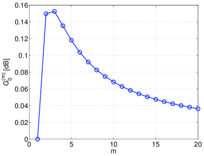
Figure 4: Gain of selection combining of $m$ transmissions in Rayleigh fading channels over a single transmission in Nakagami-$m$ fading channels, for Poisson networks with $\alpha=4$.

For Nakagami-$m$ fading, the pre-constant is $c_{m}=m^{m-1}/\Gamma(m)$, and we have

$$p_{\rm s,PPP}^{(m)}(\theta) \sim 1-c_{m}\mathbb{E}[(\theta\,\mathsf{I{\bar{S}}R})^{m}]$$

$$\lesssim 1-\frac{m^{m-1}}{\Gamma(m)}\mathsf{MISR}_{1}m!\theta^{m}$$

$$=1-\mathsf{MISR}_{1}(m\theta)^{m},$$

where ’$\lesssim$’ indicates an upper bound with asymptotic equality. Adding the second term in the lower bound and noting that

$$\mathbb{E}(h^{m})=\frac{\Gamma(2m)}{\Gamma(m)m^{m}}$$

yields the slightly sharper result

$$p_{\rm s,PPP}^{(m)}(\theta)\lesssim 1-\theta^{m}\left[\left(\frac{m\delta}{1-\delta}\right)^{m}+\frac{\delta}{m-\delta}\frac{\Gamma(2m)}{\Gamma(m)m^{m}}\right].$$

The gain for general fading is applicable to arbitrary transmission techniques that provide the same amount of diversity, not just to compare different base station deployments. As an example, we determine the gain from selection combining of the signals from $m$ transmissions over Rayleigh fading channels with a single transmission over Nakagami-$m$ fading channels, both for Poisson distributed base stations. The MISR for the selection combining scheme follows from [3, Prop. 3]. Fig. 4 shows that there is a very small gain from selection combining.

Simulation results indicate that at least for moderate $m$, the scaling $\mathsf{MISR}_{m}\approx\mathsf{MISR}_{1}(m!)^{1/m}$ holds for arbitrary motion-invariant point processes. This implies that $G_{0}^{(m)}\approx G_{0}^{(1)}$, which indicates that $G_{0}$ is insensitive to the fading statistics for small to moderate $m$. Next we show that the gain is also insensitive to the path loss exponent $\alpha$.

IV-D Insensitivity of the MISR to $\alpha$

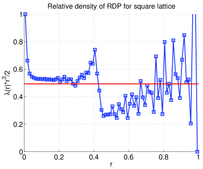
(a) Relative intensity $\lambda_{\rm sq}(r)/\lambda_{\rm PPP}(r)$ of square lattice.

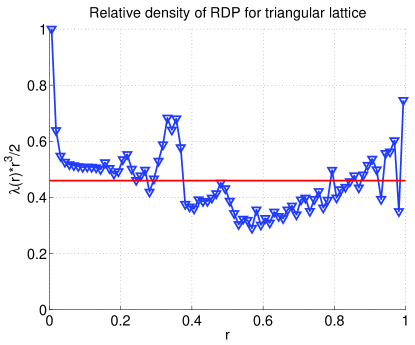
(b) Relative intensity $\lambda_{\rm tri}(r)/\lambda_{\rm PPP}(r)$ of triangular lattice.

Figure 5: Relative intensity of square and triangular lattices. The straight line is the average relative intensity and corresponds to $1/G_{0,{\rm sq}}$ and $1/G_{0,{\rm tri}}$, respectively.

Fig. 5 illustrates the densities of the square and triangular lattices relative to the PPP’s, which is $\lambda_{\rm PPP}(r)=2r^{-3}$, $r\in(0,1]$, as derived after Def. 2. Since the relative densities are roughly constant over the $[0,1]$ interval, the gains do not depend strongly on $\alpha$. Indeed, if the density of the RDP of a general point process could be expressed as $\lambda(r)=c\lambda_{\rm PPP}(r)$, we would have $G_{0}=1/c$ irrespective of $\alpha$.

Another way to show the insensitivity of the gain to $\alpha$ is by exploring the asymptotic behavior of the MISR for general point processes given in Theorem 1 in the high-$\alpha$ regime. The result is the content of the next lemma.

Lemma 5.

For a motion-invariant point process $\Phi$,

$$\mathsf{MISR}(\delta)\sim\delta\beta_{1}(1),\quad\delta\to 0,$$ (33)

where

$$\beta_{1}(1)=\frac{1}{2}\int_{\mathbb{R}^{2}}\|y_{0}\|^{2}\int\limits_{[0,2\pi]}\mathbb{E}^{!}_{y_{0},\left(\|y_{0}\|,\varphi_{1}\right)}[g(\Phi,y_{0})]\rho^{(2)}_{\Phi}\left(y_{0},\left(\|y_{0}\|,\varphi_{1}\right)\right){\rm d}\varphi_{1}{\rm d}y_{0}.$$

Proof:

The $\mathsf{MISR}$ for a general point process is given by Theorem 1 as

$$\mathsf{MISR}=2\int_{0}^{1}t^{\alpha-3}\beta_{1}(t){\rm d}t=2\int_{0}^{1}t^{-3}e^{\alpha\log(t)}\beta_{1}(t){\rm d}t.$$ (34)

Using the Laplace asymptotic technique [15, Eq. 6.419],

$$\mathsf{MISR}(\alpha)\sim 2\alpha^{-1}\beta_{1}(1),\quad\alpha\to\infty.$$

∎

This shows that $\mathsf{MISR}$ for arbitrary point processes decays as $1/\alpha$, which implies $G_{0}$ approaches a constant for large $\alpha$ (see Fig. 3(a)).

V The Expected Fading-to-Interference ratio (EFIR) and the Gain at $\infty$

In this section, we define the expected fading-to-interference ratio (EFIR) and explore its connection to the gain $G_{\infty}$ in (8). We shall see that the EFIR plays a similar role for $\theta\to\infty$ as the MISR does for $\theta\to 0$.

V-A Definition and EFIR for PPP

Definition 4 (Expected fading-to-interference ratio (EFIR)).

For a point process $\Phi$, let $I_{\infty}=\sum_{x\in\Phi}h_{x}\|x\|^{-\alpha}$ and let $h$ be a fading random variable independent of all $(h_{x})$. The expected fading-to-interference ratio (EFIR) is defined as

$$\mathsf{EFIR}\triangleq\left(\lambda\pi\mathbb{E}^{!}_{o}\left[\left(\frac{h}{I_{\infty}}\right)^{\delta}\right]\right)^{1/\delta},$$ (35)

where $\mathbb{E}^{!}_{o}$ is the expectation with respect to the reduced Palm measure of $\Phi$.

Here we use $I_{\infty}$ for the interference term, since the interference here is the total received power from all points in $\Phi$, in contrast to the interference $I$, which stems from $\Phi^{!}$.

Remark. For the PPP, the EFIR does not depend on $\lambda$, since $\mathbb{E}^{!}_{o}(I_{\infty}^{-\delta})\propto 1/\lambda$. To see this, let $\Phi^{\prime}\triangleq c\Phi$ be a scaled version of $\Phi$. Then

$$I_{c}\triangleq\sum_{x\in\Phi^{\prime}}h_{x}\|x\|^{-\alpha}=c^{-\alpha}\sum_{x\in\Phi}h_{x}\|x\|^{-\alpha}$$

and thus $I_{c}^{-\delta}=c^{2}I^{-\delta}$. Multiplying by the intensities, $\lambda_{c}I_{c}^{-\delta}=\lambda I^{-\delta}$ since $\lambda/\lambda_{c}=c^{2}$. The same argument applies to all point processes for which changing the intensity by a factor $c^{-2}$ is equivalent in distribution to scaling the process by $c$, i.e., for point processes $\Phi(\lambda)$ where $c\Phi(1)\stackrel{{\scriptstyle{\rm d}}}{{=}}\Phi(c^{-2})$. This excludes hard-core processes with fixed hard-core distance but includes lattices and hard-core processes whose hard-core distance scales with $\lambda^{-1/2}$.

Lemma 6 (EFIR for the PPP).

For the PPP, with arbitrary fading,

$$\mathsf{EFIR}_{\rm PPP}=(\operatorname{sinc}\delta)^{1/\delta}.$$ (36)

Proof:

The term $\mathbb{E}^{!}_{o}(I_{\infty}^{-\delta})$ in (35) can be calculated by taking the expectation of the following identity which follows from the definition of the gamma function $\Gamma(x)$.

$$I_{\infty}^{-\delta}\equiv\frac{1}{\Gamma(\delta)}\int_{0}^{\infty}e^{-sI_{\infty}}s^{-1+\delta}{\rm d}s.$$

Hence

$$\mathbb{E}^{!}_{o}(I_{\infty}^{-\delta})=\frac{1}{\Gamma(\delta)}\int_{0}^{\infty}\mathcal{L}^{!}_{o,I_{\infty}}(s)s^{-1+\delta}{\rm d}s.$$ (37)

From Slivnyak’s theorem [11, Thm. 8.10], $\mathbb{E}^{!}_{o}\equiv\mathbb{E}$ for the PPP, so we can replace $\mathcal{L}^{!}_{o,I_{\infty}}(s)$ by the unconditioned Laplace transform $\mathcal{L}_{I_{\infty}}(s)$, which is well known for the PPP and given by [16]

$$\mathcal{L}_{I_{\infty}}(s)=\exp(-\lambda\pi\mathbb{E}(h^{\delta})\Gamma(1-\delta)s^{\delta}).$$

From (37), we have

$$\mathbb{E}(I_{\infty}^{-\delta}) =\frac{1}{\Gamma(\delta)}\int_{0}^{\infty}e^{-\lambda\pi\mathbb{E}[h^{\delta}]\Gamma(1-\delta)s^{\delta}}s^{-1+\delta}{\rm d}s$$

$$=\frac{1}{\lambda\pi\mathbb{E}(h^{\delta})\Gamma(1-\delta)\Gamma(1+\delta)}=\frac{\operatorname{sinc}\delta}{\lambda\pi\mathbb{E}(h^{\delta})}.$$

So $\lambda\pi\mathbb{E}^{!}_{o}(I_{\infty}^{-\delta})\mathbb{E}(h^{\delta})=\operatorname{sinc}\delta$, and the result follows. ∎

Remarkably, $\mathsf{EFIR}_{\rm PPP}$ only depends on the path loss exponent. It can be closely approximated by $\mathsf{EFIR}_{\rm PPP}\approx 1-\delta$.

V-B The tail of the SIR distribution

Next we use the representation in (19) to analyze the tail asymptotics of the ccdf $\bar{F}_{\mathsf{SIR}}$ of the SIR (or, equivalently, the success probability $p_{\rm s}$).

Theorem 4.

For all simple stationary BS point processes $\Phi$, where the typical user is served by the nearest BS,

$$p_{\rm s}(\theta)\sim\left(\frac{\theta}{\mathsf{EFIR}}\right)^{-\delta},\quad\theta\to\infty.$$

Proof:

From (9), we have $p_{\rm s}(\theta)=\mathbb{E}\bar{F}_{h}(\theta R^{\alpha}I)$. Using the representation given in (19), it follows from the Campbell-Mecke theorem that the success probability equals

$$\mathbb{E}\sum_{x\in\Phi}\bar{F}_{h}\left(\theta\|x\|^{\alpha}\sum_{y\in\Phi\setminus\{x\}}h_{y}\|y\|^{-\alpha}\right)\mathbf{1}\big{(}\Phi(b(o,\|x\|))=0\big{)}\\ =\lambda\int\limits_{\mathbb{R}^{2}}\mathbb{E}_{o}^{!}\bigg{[}\bar{F}_{h}\Big{(}\theta\|x\|^{\alpha}\sum_{y\in\Phi_{x}}\!h_{y}\|y\|^{-\alpha}\Big{)}\mathbf{1}(b(o,\|x\|)\;\text{empty})\bigg{]}{\rm d}x,$$

where $\Phi_{x}\triangleq\{y\in\Phi\colon y+x\}$ is a translated version of $\Phi$. Substituting $x\theta^{\delta/2}\mapsto x$,

$$p_{\rm s}(\theta) =\lambda\theta^{-\delta}\int_{\mathbb{R}^{2}}\mathbb{E}^{!}_{o}\bigg{[}\bar{F}_{h}\Big{(}\|x\|^{\alpha}\sum_{y\in\Phi_{x\theta^{-\delta/2}}}h_{y}\|y\|^{-\alpha}\Big{)}\mathbf{1}(b(o,\|x\|\theta^{-\delta/2})\text{ empty})\bigg{]}{\rm d}x$$

$$\stackrel{{\scriptstyle(a)}}{{\sim}}\lambda\theta^{-\delta}\int_{\mathbb{R}^{2}}\mathbb{E}^{!}_{o}\bar{F}\left(\|x\|^{\alpha}I_{\infty}\right){\rm d}x,\quad\theta\to\infty$$ (38)

$$\stackrel{{\scriptstyle(b)}}{{=}}\lambda\theta^{-\delta}\mathbb{E}^{!}_{o}(I_{\infty}^{-\delta})\int_{\mathbb{R}^{2}}\bar{F}_{h}\left(\|x\|^{\alpha}\right){\rm d}x,\quad\theta\to\infty,$$

where $(a)$ follows since $\theta^{-\delta/2}\to 0$ and hence $\mathbf{1}\{b(o,\|x\|\theta^{-\delta/2})\text{ empty}\}\to 1$. The equality in $(b)$ follows by using the substitution $xI^{1/\alpha}\to x$. Changing into polar coordinates, the integral can be written as

$$\int_{\mathbb{R}^{2}}\bar{F}_{h}\left(\|x\|^{\alpha}\right){\rm d}x= \pi\delta\int_{0}^{\infty}r^{\delta-1}\bar{F}_{h}(r){\rm d}r\stackrel{{\scriptstyle(a)}}{{=}}\pi\mathbb{E}(h^{\delta}),$$

where $(a)$ follows since $h\geq 0$ [17]. Since $\mathbb{E}(h)=1$ and $\delta<1$, it follows that $\mathbb{E}(h^{\delta})<\infty$. ∎

For Rayleigh fading, from the definition of the success probability and Theorem 4,

$$p_{\rm s}(\theta)=\mathcal{L}_{\mathsf{I{\bar{S}}R}}(\theta)\sim\left(\frac{\theta}{\mathsf{EFIR}}\right)^{-\delta},\quad\theta\to\infty.$$

Hence the Laplace transform of $\mathsf{I{\bar{S}}R}$ behaves as $\Theta(\theta^{-\delta})$ for large $\theta$. Hence using the Tauberian theorem in [18, page 445], we can infer that

$$\mathbb{P}(\mathsf{I{\bar{S}}R}<x)\sim x^{\delta}\frac{\mathsf{EFIR}^{\delta}}{\Gamma(1+\delta)},\quad x\to 0.$$ (39)

From Theorem 4, the gain $G_{\infty}$ immediately follows.

Corollary 5 (Asymptotic gain at $\theta\to\infty$).

For an arbitrary simple stationary point process $\Phi$ with EFIR given in Def. 4, the asymptotic gain at $\theta\to\infty$ relative to the PPP is

$$G_{\infty}=\frac{\mathsf{EFIR}}{\mathsf{EFIR}_{\rm PPP}}=\left(\frac{\lambda\pi\mathbb{E}^{!}_{o}(I_{\infty}^{-\delta})\mathbb{E}(h^{\delta})}{\operatorname{sinc}\delta}\right)^{1/\delta}.$$

Proof:

From Theorem 4, we have that the constant $c$ in (8) is given by $c=\mathsf{EFIR}^{\delta}$. $c_{\rm PPP}$ follows from Lemma 6 as $c_{\rm PPP}=\mathsf{EFIR}_{\rm PPP}^{\delta}=\operatorname{sinc}\delta$. ∎

The Laplace transform of the interference in (37) for general point processes can be expressed as

$$\mathcal{L}^{!}_{o,I_{\infty}}(s) =\mathbb{E}^{!}_{o}\left(e^{-s\sum_{x\in\Phi}h_{x}\|x\|^{-\alpha}}\right)$$

$$=\mathbb{E}^{!}_{o}\prod_{x\in\Phi}\mathcal{L}_{h}(s\|x\|^{-\alpha})=\mathcal{G}^{!}_{o}[\mathcal{L}_{h}({s\|\cdot\|^{-\alpha}})],$$

where $\mathcal{G}^{!}_{o}$ is the probability generating functional with respect to the reduced Palm measure and $\mathcal{L}_{h}$ is the Laplace transform of the fading distribution.

Corollary 6 (Rayleigh fading).

With Rayleigh fading, the expected fading-to-interference ratio simplifies to

$$\mathsf{EFIR}=\left(\lambda\int_{\mathbb{R}^{2}}\mathcal{G}^{!}_{o}[\Delta(x,\cdot)]{\rm d}x\right)^{1/\delta},$$

where

$$\Delta(x,y)=\frac{1}{1+\|x\|^{\alpha}\|y\|^{-\alpha}}.$$

Proof:

With Rayleigh fading, the power fading coefficients are exponential, i.e., $\bar{F}_{h}(x)=\exp(-x)$. From (38), we have

$$p_{\rm s}(\theta) \sim\lambda\theta^{-\delta}\int_{\mathbb{R}^{2}}\mathbb{E}^{!}_{o}\bar{F}\left(\|x\|^{\alpha}I\right){\rm d}x$$

$$=\lambda\theta^{-\delta}\int_{\mathbb{R}^{2}}\mathbb{E}^{!}_{o}\prod_{y\in\Phi}\frac{1}{1+\|x\|^{\alpha}\|y\|^{-\alpha}}{\rm d}x,$$

and the result follows from the definition of the reduced probability generating functional. ∎

For Rayleigh fading, the fact that $\theta^{\delta}p_{\rm s}(\theta)\to\operatorname{sinc}\delta$ as $\theta\to\infty$ was derived in [8, Thm. 2].

V-C Tail of received signal strength

While Theorem 4 shows that $p_{\rm s}(\theta)=\Theta(\theta^{-\delta}),\theta\to\infty$, it is not clear, if the scaling is mainly contributed by the received signal strength or the interference. Intuitively, since an infinite network is considered, the event of the interference being small is negligible and hence for large $\theta$, the event $S/I>\theta$ is mainly determined by the random variable $S$. This is in fact true as is shown in the next lemma.

Lemma 7.

For all stationary point processes and arbitrary fading, the tail of the ccdf of the desired signal strength $S$ is

$$\mathbb{P}(S>\theta)\sim\lambda\pi\mathbb{E}(h^{\delta})\theta^{-\delta},\quad\theta\to\infty.$$

Proof:

The cdf of the distance $R$ to the nearest BS is $F_{R}(x)\sim\lambda\pi x^{2}$ for all stationary point processes [10]. Hence

$$\mathbb{P}(S>\theta) =\mathbb{P}(R<(h/\theta)^{\delta/2})$$

$$\sim\lambda\pi\mathbb{E}[(h/\theta)^{\delta}].$$

∎

So the tail of the received signal power $S$ is of the same order $\Theta(\theta^{-\delta})$, and the interference and the fading only affect the pre-constant. In the Poisson case with Rayleigh fading,

$$p_{\rm s}(\theta)\sim\lambda\pi\Gamma(1+\delta)\theta^{-\delta},\quad\theta\to\infty.$$

The same holds near $\theta=0$. If for the fading cdf, $F_{h}(x)\sim ax^{m}$, $x\to 0$,

$$\mathbb{P}(S<\theta)=\mathbb{E}F_{h}(\theta R^{\alpha})\sim a\theta^{m}\mathbb{E}(R^{m\alpha}),\quad\theta\to 0.$$

For the PPP,

$$\mathbb{P}(S<\theta)\sim\frac{\Gamma(1+m\alpha/2)}{(\lambda\pi)^{m\alpha/2}}\theta^{m},\quad\theta\to 0.$$

So on both ends of the SIR distribution, the interference only affects the pre-constant.

We now explore the tail of the distribution to the maximum SIR seen by the typical user for exponential $h$. Assume that the typical user connects to the BS that provides the instantaneously strongest SIR (as opposed to the strongest SIR on average as before). Also assume that $\theta>1$. Let $\mathsf{SIR}(x)$ denote the SIR between the BS at $x$ and the user at the origin. Then

$$\mathbb{P}(\max_{x\in\Phi}{\mathsf{SIR}(x)}>\theta) =\mathbb{E}\sum_{x\in\Phi}\mathbb{P}(\mathsf{SIR}(x)>\theta)$$

$$=\lambda\int_{\mathbb{R}^{2}}\mathbb{P}^{!}_{o}(\mathsf{SIR}(x)>\theta){\rm d}x$$

$$=\lambda\int_{\mathbb{R}^{2}}\mathcal{G}^{!}_{o}\left[\frac{1}{1+\theta(\|x\|/\|\cdot\|)^{\alpha}}\right]{\rm d}x$$

$$=\lambda\theta^{-\delta}\int_{\mathbb{R}^{2}}\mathcal{G}^{!}_{o}[\Delta(x,\cdot)]{\rm d}x.$$

From the above we observe that (for exponential fading),

$$p_{\rm s}(\theta)\sim\mathbb{P}(\max_{x\in\Phi}{\mathsf{SIR}(x)}>\theta),\quad\theta\to\infty.$$

which shows that the tail with the maximum $\mathsf{SIR}$ connectivity coincides with the nearest neighbor connectivity.

VI Examples

VI-A Lattices

Let $u_{1},u_{2}$ be iid uniform random variables in $[0,1]$. The unit intensity (square) lattice point process $\Phi$ is defined as $\Phi\triangleq\mathbb{Z}^{2}+(u_{1},u_{2})$. For this lattice, with Rayleigh fading, the Laplace transform of the interference is bounded as [19]

$$e^{-sZ(2/\delta)}\leq\mathcal{L}^{!}_{o,I_{\infty}}(s)\leq\frac{1}{1+sZ(2/\delta)},$$ (40)

where $Z(x)=4\zeta(x/2)\beta(x/2)$ is the Epstein zeta function, $\zeta(x)$ is the Riemann zeta function, and $\beta(x)$ is the Dirichlet beta function. Hence from (37)

$$Z(2/\delta)^{-\delta}\leq\mathbb{E}^{!}_{o}(I_{\infty}^{-\delta})\leq\frac{\pi\csc(\pi\delta)}{\Gamma(\delta)Z(2/\delta)^{\delta}}.$$

The upper bound equals $(Z(2/\delta)^{\delta}\Gamma(1+\delta)\operatorname{sinc}\delta)^{-1}$, and it follows that for Rayleigh fading,

$$\frac{(\pi\Gamma(1+\delta))^{1/\delta}}{Z(2/\delta)}\leq\mathsf{EFIR}_{\rm lat}\leq\left(\frac{\pi}{\operatorname{sinc}\delta}\right)^{1/\delta}\frac{1}{Z(2/\delta)}.$$ (41)

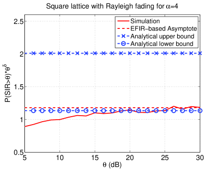
Figure 6: Scaled success probability $p_{\rm s}(\theta)\theta^{\delta}$ for the square lattice point process with Rayleigh fading and $\alpha=4$. The asymptote (dashed line) is $\sqrt{\mathsf{EFIR}}\approx 1.19$ and is tight as $\theta\to\infty$.

As $\alpha$ increases ($\delta\to 0$), the upper and lower bounds approach each other and thus both bounds get tight.

The success probability multiplied by $\theta^{\delta}$, the $\mathsf{EFIR}$ asymptote and its bounds (41) for a square lattice process are plotted in Figure 6 for $\alpha=4$. We observe that the lower bound, which is 1.29, is indeed a good approximation to the numerically obtained value $\mathsf{EFIR}\approx 1.40$, and that for $\theta>15$ dB, the ccdf is already quite close to the asymptote.

For the square and triangular lattices, Fig. 7 shows the gain as a function of $\theta$ and the asymptotic gains $G_{0}$ and $G_{\infty}$ for Rayleigh fading. Interestingly, the behavior of the gap is not monotone. It decreases first and then (re)increases to $G_{\infty}$. It appears that $G(\theta)\leq\max\{G_{0},G_{\infty}\}$. If this holds in general, a shift by the maximum of the two asymptotic gains always results in an upper bound on the SIR ccdf.

Fig. 8 shows the dependence of $G_{0}$ and $G_{\infty}$ on $\alpha$. As pointed out in Subs. IV-D, $G_{0}$ is very insensitive to $\alpha$. $G_{\infty}$ appears to increase slightly and linearly with $\alpha$ in this range.

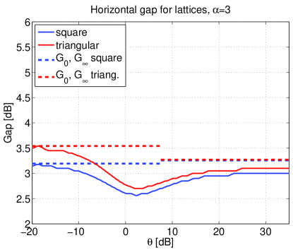
(a) $\alpha=3$

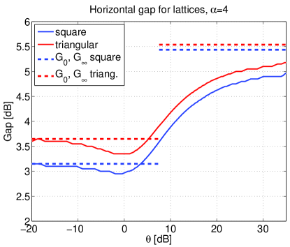
(b) $\alpha=4$

Figure 7: Gains $G(\theta)$ for the square and triangular lattices and asymptotic gains $G_{0}$ and $G_{\infty}$ (dashed) for Rayleigh fading and $\alpha=3$ and $\alpha=4$.

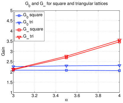
Figure 8: Asymptotic gains $G_{0}$ and $G_{\infty}$ (linear scale) for square and triangular lattices for Rayleigh fading as a function of $\alpha$.

VI-B Determinantal point processes

Determinantal (fermion) point processes (DPPs) [20] exhibit repulsion and thus can be used to model the fact that BSs have a minimum separation. The kernel of the DPP $\Phi$ is denoted by $K(x,y)$ and—due to stationarity—is of the form $K(x-y)$. Its determinants yield the product densities of the DPP, hence the name. The reduced Palm measure $\mu^{x_{o}}$ pertaining to a DPP with kernel $K^{x_{o}}$ is defined as

$$K^{x_{o}}(x,y)\triangleq\frac{1}{K(x_{o},x_{o})}\det\left(\begin{array}[]{ll}K(x,y)&K(x,x_{o})\\ K(x_{o},y)&K(x_{o},x_{o})\end{array}\right),$$ (42)

whenever $K(x_{o},x_{o})>0$. Let $K^{o}(x,y)$ denote the kernel associated with the reduced Palm distribution of the DPP process. The reduced probability generating functional for a DPP is given by [20]

$$\mathcal{G}^{!}_{o}[f(\cdot)]\triangleq\mathbb{E}^{!}_{o}\left[\prod_{x\in\Phi}f(x)\right]=\operatorname{detf}(\mathbf{1}-(1-f)K^{o}),$$ (43)

where $\operatorname{detf}$ is the Fredholm determinant and $\mathbf{1}$ is the identity operator. The next lemma characterizes the EFIR a general DPP with Rayleigh fading.

Lemma 8.

When the BSs are distributed as a stationary DPP, the EFIR with Rayleigh fading is

$$\mathsf{EFIR}=\left(\lambda\int_{\mathbb{R}^{2}}\operatorname{detf}(\mathbf{1}-(1-{\Delta}(x,\cdot))K^{o}){\rm d}x\right)^{1/\delta}.$$ (44)

Proof:

Follows from Corollary 6 and (43). ∎

Ginibre point processes: Ginibre point processes (GPPs) are determinantal point processes with density $\lambda=c/\pi$ and kernel

$$K(x,y)\triangleq\frac{c}{\pi}e^{-\frac{c}{2}(|x|^{2}+|y|^{2})}e^{cx\bar{y}}.$$

Using the properties of GPPs [21], it can be shown that

$$\mathbb{E}^{!}_{o}(e^{-sI_{\infty}})=\prod_{k=1}^{\infty}\int_{0}^{\infty}\mathcal{L}_{h}(sr^{-\alpha/2})\frac{r^{k-1}e^{-cr}}{c^{-k}\Gamma(k)}{\rm d}r,$$

from which $\mathbb{E}^{!}_{o}(I^{-\delta})$ can be evaluated using (37).

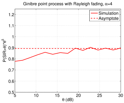
Figure 9: Scaled success probability $p_{\rm s}(\theta)\theta^{\delta}$ for the GPP for Rayleigh fading with $\alpha=4$. The asymptote (dashed line) is at $\sqrt{\mathsf{EFIR}}\approx 0.89$.

In Fig. 9, the scaled success probability $\theta^{\delta}p_{\rm s}(\theta)$ and the asymptote $\mathsf{EFIR}^{\delta}$ are plotted as a function of $\theta$ for the GPP. We observe a close match even for modest values of $\theta$. Fig. 10 shows the simulated values of the gains $G_{0}$ and $G_{\infty}$ for the GPP as a function of the path loss exponent $\alpha$. $G_{0}\approx 1.5$ for all values of $\alpha$, while $G_{\infty}\approx\alpha/2$.

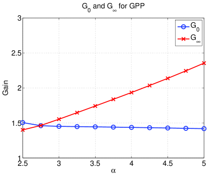
Figure 10: Simulated gains $G_{0}$ and $G_{\infty}$ for the GPP with Rayleigh fading as a function of $\alpha$.

VII Conclusions

This paper established that the asymptotics of the SIR ccdf (or success probability) for arbitrary stationary cellular models are of the form

$$p_{\rm s}(\theta)\sim 1-c_{0}\theta^{m},\;\;\;\theta\to 0;\;\;\quad p_{\rm s}(\theta)\sim c_{\infty}\theta^{-\delta},\quad\theta\to\infty$$

for a fading cdf $F_{h}(x)=\Theta(x^{m})$, $x\to 0$. Both constants $c_{0}$ and $c_{\infty}$ depend on the path loss exponent and the point process model, and $c_{0}$ also depends on the fading statistics. Depending on the point process fading may also affect $c_{\infty}$. $c_{0}$ is related to the mean interference-to-signal-ratio (MISR). For $m=1$, $c_{0}=\mathsf{MISR}$, and for $m>1$, $c_{0}$ depends on the generalized MISR. $c_{\infty}$ is related to the expected fading-to-interference ratio (EFIR) through $c_{\infty}=\mathsf{EFIR}^{\delta}$. For the PPP, $c_{\infty}=\operatorname{sinc}\delta$. The study of the MISR is enabled by the relative distance process, which is a novel type of point process that fully captures the SIR statistics. A comparison of $G_{0}$ and $G_{\infty}$ shows that a horizontal shift of the SIR distribution of the PPP by $G_{0}$ provides an excellent approximation of the entire SIR distribution of an arbitrary stationary point process.

For all the point process models investigated so far (which were all repulsive and thus more regular than the PPP), the gains relative to the PPP are between $0$ and about $4$ dB, so the shifts are relatively modest. Higher gains can be achieved using advanced transmission techniques, including adaptive frequency reuse, BS cooperation, MIMO, or interference cancellation. As long as the diversity gain of the network architecture is known and the (generalized) MISR can be calculated (or simulated), the ASAPPP method can be applied to arbitrary cellular architectures. Such extensions will be considered in future work. A generalization to heterogeneous networks (HetNets) is proposed in [22, 23]. The method can be expected to be applicable whenever the MISR is finite. This excludes networks where interferers can be arbitrarily close to the receiver under consideration while the intended transmitter is further away, such as Poisson bipolar networks.

References

- [1] R. K. Ganti and M. Haenggi, “SIR Asymptotics in General Cellular Network Models,” in 2015 IEEE International Symposium on Information Theory (ISIT’15), Hong Kong, Jun. 2015.
- [2] J. G. Andrews, F. Baccelli, and R. K. Ganti, “A Tractable Approach to Coverage and Rate in Cellular Networks,” IEEE Transactions on Communications, vol. 59, no. 11, pp. 3122–3134, Nov. 2011.
- [3] X. Zhang and M. Haenggi, “A Stochastic Geometry Analysis of Inter-cell Interference Coordination and Intra-cell Diversity,” IEEE Transactions on Wireless Communications, vol. 13, no. 12, pp. 6655–6669, Dec. 2014.
- [4] G. Nigam, P. Minero, and M. Haenggi, “Coordinated Multipoint Joint Transmission in Heterogeneous Networks,” IEEE Transactions on Communications, vol. 62, no. 11, pp. 4134–4146, Nov. 2014.
- [5] A. Guo and M. Haenggi, “Asymptotic Deployment Gain: A Simple Approach to Characterize the SINR Distribution in General Cellular Networks,” IEEE Transactions on Communications, vol. 63, no. 3, pp. 962–976, Mar. 2015.
- [6] M. Haenggi, “The Mean Interference-to-Signal Ratio and its Key Role in Cellular and Amorphous Networks,” IEEE Wireless Communications Letters, vol. 3, no. 6, pp. 597–600, Dec. 2014.
- [7] ——, “ASAPPP: A Simple Approximative Analysis Framework for Heterogeneous Cellular Networks,” Dec. 2014, Keynote presentation at the 2014 Workshop on Heterogeneous and Small Cell Networks (HetSNets’14). Available at http://www.nd.edu/~mhaenggi/talks/hetsnets14.pdf.
- [8] N. Miyoshi and T. Shirai, “A Cellular Network Model with Ginibre Configured Base Stations,” Advances in Applied Probability, vol. 46, no. 3, pp. 832–845, Aug. 2014.
- [9] B. Blaszczyszyn and H. P. Keeler, “Studying the SINR process of the typical user in Poisson networks by using its factorial moment measures,” IEEE Transactions on Information Theory, vol. 61, pp. 6774–6794, Dec. 2015.
- [10] D. Stoyan, W. S. Kendall, and J. Mecke, Stochastic Geometry and its Applications. John Wiley & Sons, 1995, 2nd Ed.
- [11] M. Haenggi, Stochastic Geometry for Wireless Networks. Cambridge University Press, 2012.
- [12] K.-H. Hanisch, “On inversion formulae for -fold Palm distributions of point processes in LCS-spaces,” Mathematische Nachrichten, vol. 106, no. 1, pp. 171–179, 1982.
- [13] W. P. Johnson, “The curious history of Faá di Bruno’s formula,” American Math. Monthly, vol. 109, pp. 217–234, Mar. 2002.
- [14] S. T. Veetil, K. Kuchi, A. K. Krishnaswamy, and R. K. Ganti, “Coverage and rate in cellular networks with multi-user spatial multiplexing,” in 2013 IEEE International Conference on Communications (ICC’13), Budapest, Hungary, Jun. 2013.
- [15] S. A. Orszag and C. Bender, Advanced mathematical methods for scientists and engineers. McGraw-Hill, 1978.
- [16] M. Haenggi and R. K. Ganti, “Interference in Large Wireless Networks,” Foundations and Trends in Networking, vol. 3, no. 2, pp. 127–248, 2008, available at http://www.nd.edu/~mhaenggi/pubs/now.pdf.
- [17] G. Folland, Real analysis: modern techniques and their applications. John Wiley & Sons, 2013.
- [18] W. Feller, An introduction to probability theory and its applications?, 2nd ed. Wiley, 1970, vol. 2.
- [19] R. Giacomelli, R. K. Ganti, and M. Haenggi, “Outage Probability of General Ad Hoc Networks in the High-Reliability Regime,” IEEE/ACM Transactions on Networking, vol. 19, no. 4, pp. 1151–1163, Aug. 2011.
- [20] J. B. Hough, M. Krishnapur, Y. Peres, and B. Virág, Zeros of Gaussian Analytic Functions and Determinantal Point Processes, ser. University Lecture Series 51. American Mathematical Society, 2009.
- [21] N. Deng, W. Zhou, and M. Haenggi, “The Ginibre Point Process as a Model for Wireless Networks with Repulsion,” IEEE Transactions on Wireless Communications, vol. 14, no. 1, pp. 107–121, Jan. 2015.
- [22] H. Wei, N. Deng, W. Zhou, and M. Haenggi, “A Simple Approximative Approach to the SIR Analysis in General Heterogeneous Cellular Networks,” in IEEE Global Communications Conference (GLOBECOM’15), San Diego, CA, Dec. 2015.
- [23] ——, “Approximate SIR Analysis in General Heterogeneous Cellular Networks,” IEEE Transactions on Communications, 2015, submitted. Available at http://www.nd.edu/~mhaenggi/pubs/tcom15b.