Large Fluctuations and Singular Behavior of Nonequilibrium Systems

Abstract

We present a general geometrical approach to the problem of escape from a metastable state in the presence of noise. The accompanying analysis leads to a simple condition, based on the norm of the drift field, for determining whether caustic singularities alter the escape trajectories when detailed balance is absent. We apply our methods to systems lacking detailed balance, including a nanomagnet with a biaxial magnetic anisotropy and subject to a spin transfer torque. The approach described within allows determination of the regions of experimental parameter space that admit caustics.

Introduction. A noisy dynamical system will occasionally experience large fluctuations that can dramatically alter its state. These fluctuations are responsible for a wide variety of interesting behaviors, including stochastic resonance stochres ; Loffstedt , transport via Brownian ratchets ratchets ; Millonas , logarithmic susceptibility in driven non-adiabatic systems SmelyanskiyPRL , and Brownian vortices Bo1 ; Bo2 . In the limit of weak noise, the system’s dynamical response is determined by its optimal paths, i.e., the paths along which it moves with maximum probability FW ; DykRev .

When the system’s stationary probability distribution lacks detailed balance, the optimal paths can exhibit unusual behavior. In particular, singularities known as caustics can develop in the action of the quasistationary density Millonas ; Dyk3 ; Maier1992 ; Maier1993b ; Kogan2011 resulting from folds and cusps in the projection of the Lagrangian manifold of escape trajectories onto the original space of the dynamical variables Dyk3 . Such singularities cannot occur in the presence of detailed balance, but in its absence their presence can significantly alter the behavior of noise-induced escape from a static metastable state Dyk3 ; Maier1993b or a limit cycle SmelyanskiyPRE ; Maier1996 . Optimal trajectories avoid caustics Dyk3 , so appearance of a caustic in the vicinity of a stable or saddle point can dramatically alter the escape behavior Maier1993b .

In this Letter, we reformulate the escape problem and in so doing determine conditions under which singularities in the optimal escape trajectories can appear. This leads to a new approach, based on a simple feature of the deterministic (i.e., zero-noise) dynamics, toward determining the presence and behavior of caustics. We apply our approach, first to a previously studied system Maier1993b in which caustics are known to dramatically affect the escape dynamics, and then to a system not studied from this perspective, namely magnetic reversal in a biaxial nanomagnet subject to both thermal noise and spin transfer torque. For the latter system we determine the experimental parameter ranges for which caustics are likely (and unlikely) to occur.

Escape in a noisy dynamical system. Consider an overdamped particle with position vector ${\mathbf{x}}(t)$ in an $n$-dimensional space. If the particle is subject to both deterministic and random forces, its time evolution in the general case is described by the Langevin equation

$$\dot{\mathbf{x}}=\mathbf{F}(\mathbf{x})+\sqrt{2\epsilon}\mathbf{\hat{H}}\cdot\dot{\mathbf{W}}\,,$$ (1)

where $\mathbf{F}(\mathbf{x})$ denotes the drift field, $\dot{\mathbf{W}}$ represents a white noise process, and the tensor $\mathbf{\hat{H}}(\mathbf{x})$ and scalar $\epsilon$ characterize the noise anisotropy and strength, respectively. We take $\epsilon$ to be sufficiently small so the timescale of a successful escape is much longer than that of a single excursion from the stable point.

Diagonalizing (1), we let $\mathbf{\hat{G}}$ be the diagonal matrix with $\hat{G}_{ii}=g_{i}^{2}$ corresponding to $\mathbf{\hat{H}}$; the associated drift field vector then has components $f_{i}=F_{i}/g_{i}^{2}$. The quasi-stationary distribution $\rho(\mathbf{x})\propto\exp[-S(\mathbf{x})/2\epsilon]$ is given to leading order in the zero-noise limit FW by the solution of the variational problem $S=\min\int_{-\infty}^{\infty}L_{FW}\;\mathrm{d}t$, with the Friedlin-Wentzell (FW) Lagrangian and associated Hamiltonian given by

$$L_{FW} = \frac{1}{2}(\dot{\mathbf{x}}-\mathbf{F})\cdot\hat{G}^{-1}\cdot(\dot{\mathbf{x}}-\mathbf{F})$$ (2)

$$H_{FW} = \frac{1}{2}\left[(\mathbf{p}+\mathbf{f})\cdot\hat{G}\cdot(\mathbf{p}+\mathbf{f})-\mathbf{f}\cdot\hat{G}\cdot\mathbf{f}\right]\,.$$ (3)

Where $\mathbf{p}$ is the FW canonical momentum with elements $p_{i}=\partial_{\dot{x}_{i}}L_{FW}$.

Suppose now that the drift field contains one or more stable fixed points, and that the system’s initial state lies within the basin of attraction of one of these. It can be seen by inspection of (3) that the fluctuational dynamics can be mapped onto the problem of a particle with unit electrical charge moving on a Riemannian manifold with (positive definite) metric tensor $\mathbf{\hat{G}}$, under the combined influence of a magnetic vector potential $\mathbf{A}=-\mathbf{f}$ Dykman1983 and electric scalar potential $\phi=-\mathbf{f}\cdot\hat{G}\cdot\mathbf{f}=-|\mathbf{f}|^{2}_{\mathbf{\hat{G}}}$ note . Hamilton’s equations of motion are then:

$$\dot{\mathbf{x}} = \hat{G}\cdot\mathbf{p}+\mathbf{F}=\hat{G}\cdot(\mathbf{p}+\mathbf{f})$$ (4)

$$\dot{\mathbf{p}} = -\nabla_{\mathbf{x}}H_{FW}\,.$$ (5)

The optimal escape paths are zero energy trajectories, that is, those along which the Hamiltonian (3) vanishes (see, for example, Maier2 ). For any state vector $\mathbf{x}$, the set of momenta satisfying the zero-energy condition $H_{FW}=0$ can be seen to describe an $n$-dimensional ellipse in momentum space centered at $\mathbf{p}=-\mathbf{f}$ and with axes $a_{i}=\sqrt{\mathbf{f}\cdot\hat{G}\cdot\mathbf{f}/g_{i}^{2}}$.

The momentum ellipse. For simplicity we now confine our considerations to two dimensions; the procedure presented below is straightforwardly generalized to higher dimensions by parametrizing an $n$-dimensional ellipse. The $2D$ momentum ellipse can be parametrized as:

$$p_{x}(\gamma) = \frac{|\mathbf{f}|_{\hat{G}}}{g_{x}}\cos\gamma-f_{x}$$ (6)

$$p_{y}(\gamma) = \frac{|\mathbf{f}|_{\hat{G}}}{g_{y}}\sin\gamma-f_{y}\,.$$ (7)

This momentum ellipse defines all possible least-action motions accessible to the particle at $\mathbf{x}$ traveling along an escape trajectory. The usual anti-instanton trajectories ($\bar{p}=0$) characterizing zero-noise drift correspond to $\gamma=\gamma_{0}\equiv-\arctan(\frac{f_{y}}{f_{x}}\frac{g_{y}}{g_{x}})$; instanton trajectories for systems satisfying detailed balance correspond to motion antiparallel to the drift fields ($\bar{p}=-2\bar{f}$) FW ; Maier2 ; Marder , which here corresponds to $\gamma=\pi+\gamma_{0}$. Fig. 1 shows a typical diagram of such a momentum ellipse.

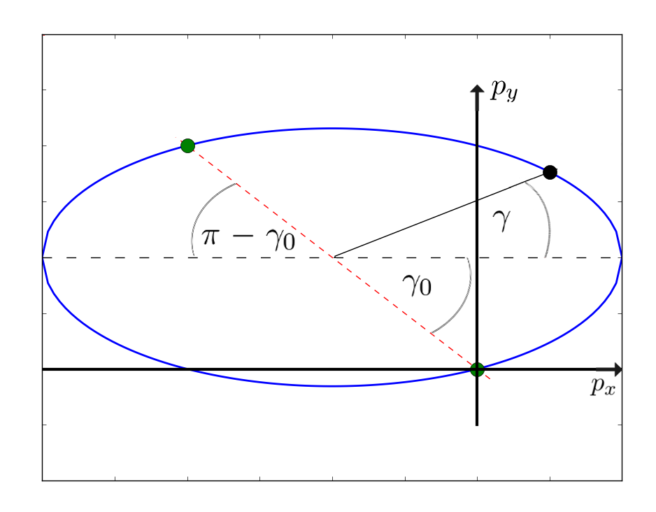
Figure 1: Diagram of momentum ellipse parametrized by $\gamma$. $\gamma_{0}$ and $\pi+\gamma_{0}$ correspond to instanton and anti-instanton solutions respectively.

Because the angle $\gamma$ parametrizes momentum at each point in configuration space, it is convenient to express the equations of motion of the particle trajectories solely as a function of $\mathbf{x}$ and $\gamma$. Substituting (6) and (7) into the Hamiltonian equations of motion (4) and (5) , we find

$$\dot{x} = g_{x}|\mathbf{f}|_{\mathbf{\hat{G}}}\cos\gamma$$

$$\dot{y} = g_{y}|\mathbf{f}|_{\mathbf{\hat{G}}}\sin\gamma.$$ (8)

The role of $\gamma$ in characterizing the direction of escape is apparent. The slope of the escape trajectory is found by dividing the second of Eqs. (Large Fluctuations and Singular Behavior of Nonequilibrium Systems) by the first to yield

$$\partial y/\partial x=(g_{y}/g_{x})\tan\gamma\,.$$ (9)

The nature of fluctuational trajectories. Eqs. (Large Fluctuations and Singular Behavior of Nonequilibrium Systems) show that thermally driven dynamics evolve at the rate of the deterministic dynamics rescaled by the noise-induced metric, i.e. $|\dot{x}|_{\mathbf{\hat{G}}^{-1}}^{2}=|\mathbf{f}|_{\mathbf{\hat{G}}}^{2}=|\mathbf{F}|_{\mathbf{\hat{G}}^{-1}}^{2}$. The two rates become trivially identical for isotropic noise ($\mathbf{\hat{G}}\equiv\mathbf{\hat{1}}$) where detailed balance is satisfied, because the instanton $\dot{\mathbf{x}}=-\mathbf{f}$ and anti-instanton $\dot{\mathbf{x}}=\mathbf{f}$ trajectories are simply sign-reversed. It is somewhat surprising, however, to see that it holds more generally. This result can alternatively be derived by writing down the effective Lorentz dynamics for a charged particle traveling in both electric and magnetic fields

$$\ddot{\mathbf{x}}=\nabla|\mathbf{f}|^{2}-\dot{\mathbf{x}}\times(\nabla\times\mathbf{f})$$ (10)

and noting that upon multiplying by $\dot{\mathbf{x}}$ one obtains $\partial_{t}|\dot{\mathbf{x}}|^{2}=\partial_{t}|\mathbf{f}|^{2}$, again implying that the dynamical speed of a particle moving under the influence of noise is equal to the norm of the zero-noise drift field. This notion has been employed in the literature Heymann2008 to construct an efficient numerical scheme (the gMAM method) capable of computing transition pathways via geometric minimization of the FW action, improving on the older String method Weinan2002 ; Ren2007 .

Using these results, the Friedlin-Wentzel Lagrangian can be rewritten as:

$$\begin{split}L_{FW}=\frac{1}{2}|\dot{\mathbf{x}}-\mathbf{F}|_{\mathbf{\hat{G}}^{-1}}^{2}&=\frac{1}{2}\left[|\dot{\mathbf{x}}|_{\mathbf{\hat{G}}^{-1}}^{2}+|\mathbf{F}|_{\mathbf{\hat{G}}^{-1}}^{2}-2\dot{\mathbf{x}}\cdot\mathbf{\hat{G}^{-1}}\cdot\mathbf{F}\right]\\ &=|\mathbf{f}|_{\mathbf{\hat{G}}}^{2}-\dot{\mathbf{x}}\cdot\mathbf{f}\\ &=|\mathbf{f}|_{\mathbf{\hat{G}}}^{2}\left(1-\cos\Psi\right)\end{split}$$ (11)

where we have employed the identities $\mathbf{F}=\mathbf{\hat{G}}\cdot\mathbf{f}$ and $\dot{\mathbf{x}}\cdot\mathbf{\hat{G}}^{-1}\cdot\dot{\mathbf{x}}=|\mathbf{f}|_{\mathbf{\hat{G}}}^{2}$, and defined

$$\Psi\equiv\mathrm{arccos}\left(\frac{\dot{\mathbf{x}}\cdot\mathbf{f}}{|\mathbf{f}|_{\mathbf{\hat{G}}}^{2}}\right)$$ (12)

as the angle between the instantaneous escape velocity $\dot{\mathbf{x}}$ and the deterministic drift field $\mathbf{f}$ at $\mathbf{x}$. Eq. (12) shows that, as long as $\Psi$ does not vary too much over the course of the escape trajectory, the effective action $S(\mathbf{x})=\int_{-\infty}^{\infty}L_{FW}dt$ will be dominated by the behavior of $|\mathbf{f}|_{\mathbf{\hat{G}}}$, implying that the norm of the drift field alone captures much of the structure of the system’s action. This is the central result of the paper.

To characterize better the relative importance of $|\mathbf{f}|$ vs. $\Psi$ on the escape dynamics, consider a closed fluctuational path ${\cal C}$ that moves from a stable fixed point $\mathbf{x_{S}}$ to some other point $\mathbf{x_{0}}$ within its attractive basin, subsequently returning (along the anti-instanton trajectory $\dot{\mathbf{x}}=\mathbf{f}$) to the fixed point. Using $\mathbf{\Omega_{\cal C}}$ to denote the surface enclosed by $\mathbf{\cal C}$, we find

$$S_{\cal C}=\oint_{\cal C}\left(|\mathbf{f}|_{\mathbf{\hat{G}}}^{2}-\dot{\mathbf{x}}\cdot\mathbf{f}\right)\mathrm{d}t=\oint_{\cal C}\mathrm{d}s|\mathbf{f}|_{\mathbf{\hat{G}}}-\int\mathrm{d}\mathbf{\Omega_{\cal C}}\cdot\left(\nabla\times\mathbf{f}\right)\,.$$ (13)

In the second equality we changed integration variables from $t$ to $s$, where $s$ denotes distance traveled along the trajectory, and used the earlier result that $|\dot{\mathbf{x}}|=|\mathbf{f}|$ for all systems. We also used Stokes’ theorem to rewrite the effect of the geometrical phase due to $\Psi$ in terms of its equivalent surface integral. This equation shows how the presence of a nongradient field (which possesses nonzero curl) contributes to the action, and therefore helps determine the trajectory, of an optimal path. While enclosing a larger ‘magnetic flux’ $\int\mathrm{d}\mathbf{\Omega_{\cal C}}\cdot(\nabla\times\mathbf{f})$ acts to reduce the path’s action (where the flux term is positive), doing so can also move the particle into regions of configuration space with larger $|\mathbf{f}|$, which acts to increase the action. The least action trajectory therefore optimizes the relative balance between these two terms.

There are two immediate consequences of (13). The first is that in gradient systems, where $\mathbf{f}=-\mathbf{\nabla}_{\mathbf{x}}{U}$ for some smooth potential function $U(\mathbf{x})$ (so $\nabla\times\mathbf{f}=0$), and where the instanton trajectory satisfies $\dot{\mathbf{x}}=-\mathbf{f}$, we recover the well-known action (see, for example, Maier2 ) for the entire trajectory: $S_{\cal C}=2\Big{[}U(\mathbf{x_{0}})-U(\mathbf{x_{S}})\Big{]}$. The second, more general consequence is that any sudden change in $|\mathbf{f}|$, as system parameters are varied, can dramatically alter the balance between the drift norm and the magnetic flux, and hence the structure of the optimal paths.

Applications. It has been observed Maier1993b ; Dyk3 that noisy systems with nongradient deterministic dynamics containing tunable parameters can dramatically change their escape behaviors, in a way reminiscent of a broken symmetry transition, when certain critical parameter thresholds are crossed. Consider, for example, the following well-studied system Maier1993b with a tunable parameter $\alpha$:

$$\dot{x} = x(1-x^{2}-\alpha y^{2})+\sqrt{\epsilon}\dot{W}_{x}$$ (14)

$$\dot{y} = -y(1+x^{2})+\sqrt{\epsilon}\dot{W}_{y},$$ (15)

where the additive white noise is isotropic and the drift field is nongradient for all $\alpha\neq 1$. For any $\alpha$, the system has two stable fixed points at $(\pm 1,0)$ and one hyperbolic (saddle) fixed point at $(0,0)$. We consider the optimal escape trajectory from $(1,0)$ to $(0,0)$, which flows along the $x$-axis for $\alpha<4$. Above $\alpha=4$, however, caustics appear in the basin of attraction of the stable point Maier1993b , focusing to a point on the $x$-axis between 0 and 1, as shown in Fig. 2. As a consequence, the optimal escape trajectory bifurcates into two off-axis trajectories.

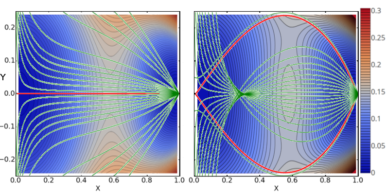
Figure 2: Contour plot of the norm of the drift field from Maier1993b , for $\alpha=3$ (left) and $\alpha=5$ (right). Optimal escape trajectories are shown in red, and other instanton trajectories in green. For $\alpha=3$, instanton trajectories do not cross, and the escape trajectory lies along the $x$-axis. Correspondingly, two global minima in the norm of the drift field are present at the unstable $(0,0)$ and stable $(1,0)$ equilibria, respectively, along with a saddle close to the midpoint of the x-axis. For $\alpha=5$, instanton trajectories cross, indicating the presence of a caustic (not shown). Correspondingly, the saddle in the norm of the drift field for $\alpha=3$ is now a local maximum, with two new local minima appearing off the $x$-axis. Consequently, there are now two symmetrical off-axis optimal escape trajectories that follow the new off-axis minima in the norm of the drift field (and in so doing avoid the caustic).

Analysis of the norm of the drift field reveals that in transitioning across the critical threshold $\alpha_{C}=4$, the structure of the extrema of $\mathbf{f}$ changes abruptly. For $\alpha<4$, the norm exhibits two global minima at $(1,0)$ and $(0,0)$, along with a saddle near the midpoint of the $x$-axis. For $\alpha>4$, however, two local minima appear symmetrically displaced off the $x$-axis, with the previous on-axis saddle now a local maximum (Fig. 2). According to (11), these new minima lower the effective action of off-axis escape trajectories, in accordance with observations. Deviation of the escape trajectories from the exact minima are due to the ‘magnetic flux’ term in (13).

A more interesting application is to a physically relevant model lacking detailed balance: the stochastic Landau-Lifshitz-Gilbert-Slonczewski (sLLGS) equation governing the evolution of a unit magnetization vector subject to a combination of both gradient and non-gradient torques. This equation reads:

$$\dot{m}_{i}=A_{i}(\mathbf{m})+B_{ik}(\mathbf{m})\circ H_{th,k},$$ (16)

where the drift vector $\mathbf{A}(\mathbf{m})$ and diffusion matrix $\hat{\mathbf{B}}(\mathbf{m})$ are given by

$$\mathbf{A}(\mathbf{m}) = \mathbf{m}\times\mathbf{h}_{\mathrm{eff}}-\alpha\mathbf{m}\times\left(\mathbf{m}\times\mathbf{h}_{\mathrm{eff}}\right)$$ (17)

$$- \alpha I\mathbf{m}\times\left(\mathbf{m}\times\mathbf{\hat{n}}_{p}\right),$$

$$B_{ik}(\mathbf{m}) = \sqrt{C}[-\epsilon_{ijk}m_{j}-\alpha(m_{i}m_{k}-\delta_{ik})]$$ (18)

and the equation is interpreted in the Stratonovich sense. The first term in $\mathbf{A}(\mathbf{m})$ corresponds to magnetization precession about a local magnetic field, with $\mathbf{h}_{\mathrm{eff}}=-\nabla_{\mathbf{m}}\epsilon(\mathbf{m})$ a conservative vector field. Here $\epsilon(\mathbf{m})$ is the energy landscape of the magnetic system under study. The second term in $\mathbf{A}(\mathbf{m})$ is a phenomenological damping term, with the damping constant $\alpha$ typically $\sim O(10^{-2})$. The third is a nongradient term corresponding to spin-angular momentum per unit time injected via a current $I$ into the macrospin along an arbitrary polarization direction $\mathbf{\hat{n}}_{p}$ notealpha . Although the diffusion matrix $\hat{\mathbf{B}}(\mathbf{m})$ (with $C$ the diffusion constant) appears state-dependent, it can be shown (e.g., by rewriting the dynamics in spherical coordinates) to correspond to isotropic, state-independent noise.

In the absence of applied currents ($I=0$), the fluctuational trajectories are determined by the energy landscape $\epsilon(\mathbf{m})$ and do not cross. In the presence of a nonvanishing current $I$, however, detailed balance is absent, and it therefore becomes important to determine how this new feature may — or may not — alter the escape dynamics. The methods developed above allow us to analyze this problem by examining the norm of the total drift field governing the macrospin dynamics. To lowest order in $\alpha$, it is

$$|\mathbf{A}(\mathbf{m})|^{2}=|\mathbf{m}\times\mathbf{h}_{\mathrm{eff}}|^{2}+2\alpha I\,\mathbf{\hat{n}}_{p}\cdot(\mathbf{m}\times\mathbf{h}_{\mathrm{eff}})+O(\alpha^{2})\,.$$ (19)

We wish to determine under which conditions the conservative precessional contribution dominates the nongradient contribution. When this occurs, the extrema of $|\mathbf{A}(\mathbf{m})|^{2}$ corresponding to $I=0$ do not change significantly when $I>0$. By the approach developed above, this implies that the most probable escape paths should not differ significantly from the reverse-drift instanton paths of the purely gradient case.

We consider for simplicity the case of a biaxial macrospin subject to the energy landscape

$$\epsilon(\mathbf{m})=Dm_{x}^{2}-m_{z}^{2}\,,$$ (20)

defined on the surface of the unit sphere ($|\mathbf{m}|=1$). Here $D\geq 0$ is the ratio of hard axis to easy axis anisotropies Pinna2013 ; PSK14 .

The calculation analyzing the relative contributions of the gradient and nongradient terms in (19) is done in detail in the Supplementary Notes supp . We find that the presence of caustics is determined by the fixed tilt angle $\omega$ that $\mathbf{\hat{n}}_{p}$ makes with the $z$-axis. For any $D$, the escape dynamics are unaffected by caustics for a wide energy range in the small tilt case ($\tan\omega\ll\alpha^{-1}$), but in principle the large tilt case ($\tan\omega\gg\alpha^{-1}$) can show substantially different behavior.

We tested these predictions by numerically integrating the FW dynamics associated with the stochastic process (16) for several different cases. Results for $D=0$ are shown in the Supplementary Notes supp . The absence of caustics, for both zero and small tilt, is apparent. Here we present the more interesting case of nonvanishing $D$. Fig. 3 shows results for $D=20$, $I=0.8\,I_{C}$, and three tilts $\omega=0$, $0.1$ and $0.25\,\theta_{C}$, where $\theta_{C}=\arctan(1/\sqrt{D})$ supp and $I_{C}$ is the critical applied current above which the entire $m_{z}>0$ region becomes unstable, eliminating the bistability of the magnetic system. These tilt values (and even larger ones) can be realized in current experiments on orthogonal spin-valve devices Li . The optimal trajectories change as tilt is increased, even though the exit point remains essentially unchanged. However, numerical results for larger tilts, up to the critical tilt, do not exhibit crossing of escape trajectories, suggesting that caustics have not formed near escape paths. The only major difference is the number of precessions the system undergoes before reaching the separatrix (i.e., the boundary of the domain of attraction of the stable fixed point, which here corresponds to $\epsilon=0$ supp ).

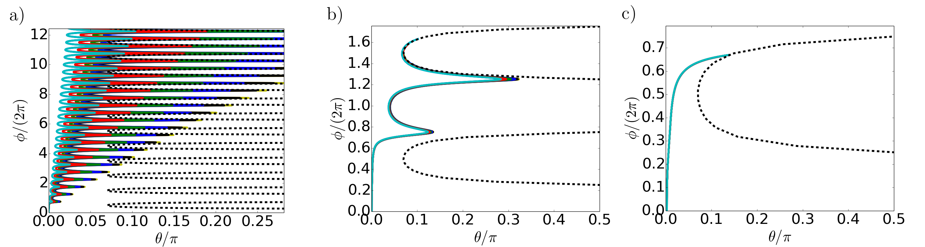
Figure 3: Escape trajectory for macrospin model with $\alpha=0.01$, $D=20$, $I=0.8\,I_{C}$ and varying tilts: (a) $\omega=0$, (b) $\omega=0.1\,\theta_{C}$, (c) $\omega=0.25\,\theta_{C}$. Different color trajectories correspond to different initial conditions of the FW dynamics. Dashed black lines correspond to the $\epsilon=0$ separatrices. In all scenarios, escape trajectories never cross, indicating the absence of caustics.

To summarize, an analysis of the norm of the drift field indicates that for most tilts, caustics do not appear within the escape region, and so — perhaps surprisingly — the loss of detailed balance does not qualitatively alter the escape dynamics. However, on closer examination one finds that for any tilt, there remain regions — where $m_{z}\approx 1$ or, separately, where $\epsilon\approx 0$ — where this conclusion breaks down, because the precessional contribution to the drift norm vanishes at $m_{z}=1$ and at $\epsilon=0$. That is, two regions will always exist in the magnet’s configuration space where the (nongradient) spin transfer torque term dominates the (gradient) precessional term. We compute the width of these regions in the Supplementary Notes and show that they are sufficiently small that their effect on the escape dynamics is negligible.

In the case when the tilt is large ($\tan\omega\gg\alpha^{-1}$), however, the nongradient term dominates the gradient term in all of configuration space, and so caustics may appear. In order to determine whether they do requires a more lengthy analysis, in which the fixed point structure of the drift field norm must be analyzed to determine whether it changes. We defer such an analysis to future work.

- (1) L. Gammaitoni, P. Hänggi, P. Jung, F. Marchesoni, Rev. Mod. Phys. 70, 223–87 (1998).
- (2) R. Löfstedt and S.N. Coppersmith, Phys. Rev. Lett. 72, 1947 (1994).
- (3) M.O. Magnasco, Phys. Rev. Lett. 71, 1477 (1993).
- (4) M. Millonas and M.I. Dykman, Phys. Lett. A 185, 65 (1994).
- (5) V.N. Smelyanskiy, M.I. Dykman, H. Rabitz, and B.E. Vugmeister, Phys. Rev. Lett 79, 3113 (1997).
- (6) B. Sun, J. Lin, E. Darby,A.Y. Grosberg and D.G. Grier, Phys. Rev. E 80, 010401R (2009).
- (7) B. Sun, D.G. Grier and A.Y. Grosberg, Phys. Rev. E 82, 021123 (2010).
- (8) M. I. Freidlin and A. D. Wentzell Random Perturbations of Dynamical Systems (Springer, New York, 1984).
- (9) M.I. Dykman and K. Lindenberg, Contemporary problems in statistical physics, p. 41, G. Weiss (SIAM, Philadelphia, 1994).
- (10) M.I. Dykman, M. Millonas and V.N. Smelyanskiy, Phys. Lett. A 195, 53 (1994).
- (11) R.S. Maier and D.L. Stein, Phys. Rev. Lett. 69, 3691 (1992).
- (12) R.S. Maier and D.L. Stein, Phys. Rev. Lett. 71, 1783 (1993).
- (13) O. Kogan, arXiv:1110.2820 (2011).
- (14) V.N. Smelyanskiy, M.I. Dykman, and R.S. Maier, Phys. Rev. E 55, 2369 (1997).
- (15) R.S. Maier and D.L. Stein, Phys. Rev. Lett. 77, 4860 (1996).
- (16) M.I. Dykman and M.A. Krivoglaz, in Synergetics and Cooperative Phenomena in Solids and Macromolecules (Valgus, Tallin 1983), pp. 33-44.
- (17) Given a Riemannian metric , we will denote the inner product of two vectors and as . Analogously, the inner product on of a vector with itself will be written .
- (18) R.S. Maier and D.L. Stein, Phys. Rev. E 48, 931 (1993).
- (19) M. Marder, Phys. Rev. Lett. 74, 4547 (1995).
- (20) M. Heymann and E. Vanden-Eijnden, Phys. Rev. Lett. 100, 140601 (2008).
- (21) W. E, W. Ren and E. Vanden-Eijnden, Phys. Rev. B 66, 052301 (2002).
- (22) W. E, W. Ren and E. Vanden-Eijnden, J. Chem. Phys 126, 164104 (2007).
- (23) The usual formulation of the spin-torque term does not include a factor of ; it is not a dissipative term. We include it here because it is convenient to define the current in terms of : , where is the spin current pumped into the system per unit time. The reason for doing this is so the critical current for switching (defined in the text two paragraphs below Eq. (20)) is independent of : .
- (24) D. Pinna, A.D. Kent and D.L. Stein, Phys. Rev. B 88, 104405 (2013).
- (25) D. Pinna, D.L. Stein, and A.D. Kent, Phys. Rev. B 90, 174405 (2014).
- (26) See Supplemental Material at [URL will be supplied by publisher] for (S1) the analysis leading to the conclusions concerning the conditions under which an applied current can qualitatively alter the escape dynamics of a biaxial macrospin system, and (S2) the analytic solution of the case in the presence of an applied current.
- (27) L. Ye, G. Wolf, D. Pinna, G.D. Chaves, A.D. Kent, arXiv:1408.4494 (2014).