Scaling properties of generalized two-dimensional Kuramoto-Sivashinsky equations

Abstract

This paper presents numerical results for the two-dimensional isotropic Kuramoto-Sivashinsky equation (KSE) with an additional nonlinear term and a single independent parameter. Surfaces generated by this equation exhibit a certain dependence of the average saturated roughness on the system size that indicates power-law shape of the surface spectrum for small wave numbers. This leads to a conclusion that although cellular surface patterns of definite scale dominate in the range of short distances, there are also scale-free long-range height variations present in the large systems. The dependence of the spectral exponent on the equation parameter gives some insight into the scaling behavior for large systems.

I Introduction

The Kuramoto-Sivashinsky equation (KSE) in its dimensionless form for some field $h$ can be written as article:sivashinsky_1979 ; article:kuramoto_tsuzuki_1976 ; article:procaccia_et.al_1992 ; article:jayaprakash_et.al_1993

$$\partial_{t}h=-\nabla^{2}h-\nabla^{4}h+(\nabla h)^{2}\,.$$ (1)

This equation stands as a paradigmatic model for chaotic spatially extended systems and can be used to study the connections between chaotic dynamics at small scales and apparent stochastic behavior at large scales. It is an example of an extended, deterministic dynamical system that exhibits complex spatio-temporal phenomena. The KSE has been derived for the purpose of describing the intrinsic instabilities in laminar flame fronts article:sivashinsky_1979 and phase-dynamics in reaction-diffusion systems article:kuramoto_tsuzuki_1976 . The equation (1) in one- and two-dimensional cases has been a subject of active research for about three decades, and its scaling properties have even been an object of some controversy article:procaccia_et.al_1992 ; article:jayaprakash_et.al_1993 .

This paper presents some results obtained from a less researched generalized version of KSE. There have been many different generalizations of the KSE used for different purposes. Some of them involve adding damping terms to (1) article:sivashinsky_1979 ; article:paniconi_et.al_1997 , some introduce spatial anisotropy article:krug_et.al_1995 or additive random noise article:lauritsen_et.al_1996 .

In the case presented here, there is an additional nonlinear term $\nabla^{2}(\nabla h)^{2}$ introduced to the KSE (1). The two-dimensional generalized Kuramoto-Sivashinsky equation of this form with an additive Gaussian white noise has been used as a model equation for amorphous solid surface growth article:linz_et.al_exp_2000 ; article:linz_et.al_2001 . The equation in this model originally has five parameters that are needed in order to reproduce the experimental data in the simulations and to examine the correspondence with microscopic properties of the surface growth process article:linz_et.al_exp_2000 . However, for theoretical investigations of the long-time and large-scale behavior of the system, the noise term can be neglected and the remaining deterministic equation can be rescaled into the dimensionless form with only one independent parameter $\alpha$:

$$\partial_{t}h=-\nabla^{2}h-\nabla^{4}h-\alpha\nabla^{2}(\nabla h)^{2}+(\nabla h)^{2}\,.$$ (2)

Equation (2) has also been used as a model for nano-scale pattern formation induced by ion beam sputtering article:cuerno_et.al_2006 ; article:cuerno_et.al_2011 .

The two-dimensional generalized Kuramoto-Sivashinsky equation (GKSE) (2) in the context of this paper describes the evolution of a (2+1)-dimensional surface, i.e., a surface which is defined as a function on a two-dimensional plane and is growing in the direction perpendicular to that plane. The surface profile $h(\boldsymbol{r},t)$ is defined as the surface height $h$ at the position $\boldsymbol{r}=(x,y)$ on the square $[0,L]^{2}$ of size $L$ in the plane $\mathbb{R}^{2}$ at time $t$ or, more generally, as a function:

$$h:\quad[0,L]^{2}\times\mathbb{R}^{+}\rightarrow\mathbb{R}\,.$$ (3)

We solve the equation (2) for different values of the parameter $\alpha$ using the finite difference method with periodic boundary conditions, the time step $\Delta t=0.005$, spatial discretization step $\Delta x=0.71086127010534\,$. Such a seemingly bizarre number for the discretization step $\Delta x$ is actually a good approximation of the value that is needed in order for the system with periodic boundary conditions to be able to contain ordered patterns that appear in some other versions of the generalized KSE. The equation is solved for system sizes $L$ ranging from about 45 to about 1000 (i.e., on the $N\times N$ lattices with $N$ from 63 to 1400, where $L=N\,\Delta x$) and in two cases up to about 1422 ($N=2000$). The methods of numerical solution for (2) are presented and compared in article:linz_et.al_numerik_2002 .

II Kinetics of the surface roughness

The surface roughness $w(t)$, also called the surface width, is one of the most important characteristics of a surface book:barabasi . It is defined as the standard deviation, or, synonymously, root mean square (rms) deviation, of the surface height $h(\boldsymbol{r},t)$ from its average value $\bar{h}(t):=\langle h(\boldsymbol{r},t)\rangle_{\boldsymbol{r}}$, at some time $t$:

$$w(t):=\sqrt{\Big{\langle}\big{(}h(\boldsymbol{r},t)-\bar{h}(t)\big{)}^{2}\Big{\rangle}_{\boldsymbol{r}}}\,.$$ (4)

Here and throughout the whole paper we denote the averaging by $\langle\cdots\rangle$ with some subscript that shows over what entities the averaging takes place. $\langle\cdots\rangle_{\boldsymbol{r}}$ denotes spatial average over the whole surface, $\langle\cdots\rangle_{t}$ temporal average, $\langle\cdots\rangle_{\eta}$ ensemble average, $\langle\cdots\rangle_{|\boldsymbol{r}|=r}$ spatial average over all $\boldsymbol{r}$ whose length is $r$ etc.

For smaller values of parameter $\alpha$ (say, $\alpha<5$) the kinetics of $w(t)$ due to the evolution of the surface resulting from (2) seems to follow a distinct pattern. Starting from a random surface with some small initial roughness $w(t=0)\ll 1$, the roughness begins to grow almost exponentially, but at some time $t_{\times}\approx 100$ this growth slows down and later on crosses over to a stationary regime where it oscillates about its average (saturation) value $w_{\mathrm{sat}}$ (see Fig. 1).

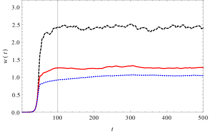
Figure 1: Kinetics of the surface roughness $w(t)$ for short times ($t<500$) for surfaces with initial roughness $w(0)=10^{-4}$ evolving according to (2) with parameter values $\alpha=0$ (black, dashed line), $\alpha=0.5$ (red, continuous line), $\alpha=1$ (blue, dotted line). System size $L\approx 355$ (in lattice units, $N=500$).

In the saturation regime, the dynamics of $w(t)$ becomes a statistically stationary process with time independent average and other statistical characteristics that are the same for different realizations (different realizations differ in the initial surface profile, as the evolution equation itself is deterministic). However, in order to consider the long time behavior (after saturation) of a statistically stationary process, it is important to take time averages over sufficiently long time intervals, having in mind that the minimal required averaging time must be at least several times longer than the correlation time of the process, defined as the time lag value at which the normalized autocorrelation function of $w(t)$ effectively falls to zero. This correlation time might strongly depend on the parameter $\alpha$ and the system size $L$.

In the stationary regime the roughness is chaotically oscillating about some average value which we denote $w_{\mathrm{sat}}$ and call saturated roughness. This value is calculated as the time average of $w(t)$ in the stationary regime and is virtually the same when averaged over different time intervals of the stationary regime (given that these intervals are sufficiently long) and for different realizations.

This saturated surface roughness can be theoretically defined as a time average over an time interval of length $T$ that goes to infinity, starting from the time $t_{0}$ where the saturation regime is surely reached:

$$w_{\mathrm{sat}}=\lim_{T\rightarrow\infty}\big{\langle}w(t)\big{\rangle}_{t\in[t_{0},\,t_{0}+T)}\,.$$ (5)

Our numerical investigation shows that, for system sizes $N$ and parameter values $\alpha$ considered in this paper, it is sufficient to take $t_{0}\geq 3000$ and $T\geq 10000$ to get the saturation values $w_{\mathrm{sat}}$ that differ less than $5\%$ for different realizations. For most of the results presented here, we have used the values $w_{\mathrm{sat}}$ obtained using $t_{0}\geq 9000$ and $T=11000$ and, furthermore, we used the averaged values of several (from 3 to 10) realizations:

$$w:=\Big{\langle}\big{\langle}w(t)\big{\rangle}_{t\in[9\cdot 10^{3},2\cdot 10^{4}]}\Big{\rangle}_{\eta}\,.$$ (6)

In this paper we are interested in the surface patterns produced by GKSE (2) and the dependence of the saturated surface roughness on parameter $\alpha$ and system size $L$.

III Resulting surfaces

The surfaces, generated by Eq. (2) in the stationary regime have a disordered cellular structure with cells whose sizes are in a quite narrow interval (see Figs. 2–4). The resulting patterns seem to have similar appearance for different system sizes $L$ (for sizes that are at least several times larger than the typical cell diameter).

The usual way to investigate the surface patterns is by calculating the surface height correlation function $C(\boldsymbol{r})$, which is the two-dimensional autocorrelation function of the surface height $h(\boldsymbol{r})$:

$$C(\boldsymbol{r})=\big{\langle}(h(\boldsymbol{r^{\prime}})-\bar{h})\,(h(\boldsymbol{r^{\prime}}+\boldsymbol{r})-\bar{h})\big{\rangle}_{\boldsymbol{r^{\prime}}}\,.$$ (7)

Since the equation (2) is isotropic, the correlation functions (7) $C(\boldsymbol{r})$ of the resulting surfaces should statistically be independent of the direction of $\boldsymbol{r}$ and, thus, depend only on its absolute value $r=|\boldsymbol{r}|$. We therefore define the isotropic height correlation function $C(r)$ as averaged over all directions of $\boldsymbol{r}$:

$$C(r)=\Big{\langle}\big{\langle}(h(\boldsymbol{r^{\prime}})-\bar{h})\,(h(\boldsymbol{r^{\prime}}+\boldsymbol{r})-\bar{h})\big{\rangle}_{\boldsymbol{r^{\prime}}}\Big{\rangle}_{|\boldsymbol{r}|=r}\,.$$ (8)

Fig. 2 shows resulting surface patterns for system size $L\approx 178$ (or, in lattice units, $N=250$) and different values of parameter $\alpha$ in (2) and the corresponding normalized height correlation functions (8). We see that for the surfaces generated by (2) with $\alpha=0$, corresponding to the KSE (1) case, the height correlation function (8) has no maximum (right panel of Fig. 2), just an area of slower decay at distances $r$ corresponding to the approximate sizes of cells in the pattern. For $\alpha>0$, the height correlation function obtains a maximum whose distance corresponds to the average size of cells. We see that this the distance of this maximum increases with $\alpha$, meaning that the cell size increases as the parameter $\alpha$ is increased.

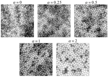
Figure 2: Left panel: Surfaces $h(\boldsymbol{r},t)$ (values of $h$ coded in gray-scale) evolving according to (2) at system size $N=250$ ($L\approx 178$) with parameters $\alpha=0,\,0.25,\,0.5,\,1,\,2$ at time $t=5000$ (in the stationary regime). Right panel: Normalized autocorrelation functions $C(r)$ as defined in (7) of the surfaces that are shown on the left panel.

Another thing that can be seen in Fig. 2 is that the normalized correlation functions $C(r)/w^{2}$ decrease slowly for small values of $\alpha\geq 0$ and faster for larger values. That is the first indication of the influence of parameter $\alpha$ on long-range height correlations.

Large-scale height variations in surfaces produced by Eq. (2) become more distinct as the system size is chosen to be many times larger than the typical cell size. The examples for some values of $\alpha$ can be seen in Fig. 3 and Fig. 4.

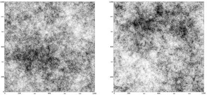
Figure 3: Surfaces (values of $h$ coded in gray-scale) at system size $N=1200$ ($L\approx 853$) evolving according to (2) with parameters $\alpha=0$ (left panel) and $\alpha=0.25$ (right panel) at time $t=6000$ (in the stationary regime).

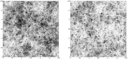
Figure 4: Surfaces (values of $h$ coded in gray-scale) at system size $N=1200$ ($L\approx 853$) evolving according to (2) with parameters $\alpha=0.5$ (left panel) and $\alpha=1$ (right panel) at time $t=6000$ (in the stationary regime).

By repeating the simulations with different system sizes $L$, one notices a slight dependence of the average saturation value of the surface roughness $w_{\mathrm{sat}}$ on the system size. Indeed, the results show that the resulting roughness increases when the system size is increased. This shows that the resulting surface profile contains spatial Fourier components of ever smaller wave number $k$ (and correspondingly larger wavelength $\lambda$). Although for small scales (large wave numbers) the structures of definite size occur, for larger distances (small wave numbers) we get the height variations with long-range dependence, and (as will be shown in the next two sections) this dependence has a scale free character.

IV Power-law surface spectra and scaling of roughness

This section presents some general considerations about the spatial power-spectral densities (PSD) of surfaces, their connection to the surface roughness $w$, and the effects introduced by the finite system size. The scaling behavior of $w$ when the PSD has a power-law shape is derived. These theoretical results are compared to the numerically calculated scaling properties of $w$ for the surfaces generated by (2) in the next section.

IV.1 Surface PSD and roughness

A two-dimensional surface $h(\boldsymbol{r})$ is a single valued function on the plane $\boldsymbol{r}=(x,y)\in\mathbb{R}^{2}$. In order to avoid the zero frequency component in the spectrum, we calculate the spectrum of the surface profile $h_{c}(\boldsymbol{r})$ with zero mean:

$$h_{c}(\boldsymbol{r}):=h(\boldsymbol{r})-\bar{h}\,,$$ (9)

where $\bar{h}\equiv\langle h(\boldsymbol{r})\rangle_{\boldsymbol{r}}$ is the average height of the surface. Fourier transformation $H(\boldsymbol{k})$ of this ’centered’ surface profile $h_{c}(\boldsymbol{r})$:

$$H(\boldsymbol{k})=\int\mathrm{d}^{2}\boldsymbol{r}\,h_{c}(\boldsymbol{r})\,\exp(-\mathrm{i}\boldsymbol{k}\cdot\boldsymbol{r})\,.$$ (10)

Here $\boldsymbol{k}=(k_{x},k_{y})^{T}$ is the wave vector of spatial Fourier components of the surface profile.

The surface power-spectral density (PSD) is then defined as:

$$S_{\boldsymbol{k}}=\frac{1}{L^{2}}|H(\boldsymbol{k})|^{2}\,,$$ (11)

where $L$ is the size of the segment of the surface analyzed, i.e., $\boldsymbol{r}\in[0,L]^{2}$. The integral of the power spectrum $S_{\boldsymbol{k}}$ over all $\boldsymbol{k}$ is equal to the variance of the surface height $\sigma_{h}^{2}$ which by our definition is is equal to the square of the surface roughness $w^{2}$:

$$\frac{1}{(2\pi)^{2}}\int\mathrm{d}^{2}\boldsymbol{k}\,S_{\boldsymbol{k}}=\sigma_{h}^{2}\equiv w^{2}\,.$$ (12)

Since our model is isotropic, $S_{\boldsymbol{k}}$ must depend only on the absolute value $|\boldsymbol{k}|$, and we can get the one-dimensional power spectrum $S(k)$ of the surface by integrating the two-dimensional power spectrum over all wave vectors $\boldsymbol{k}$ of the same absolute value $k$. This can be done by expressing the wave vector $\boldsymbol{k}$ in the polar coordinates $\boldsymbol{k}=(k,\phi)$, and then integrating $S_{\boldsymbol{k}}$ over all angles $\phi$:

$$\frac{1}{(2\pi)^{2}}\int\mathrm{d}^{2}\boldsymbol{k}\,S_{\boldsymbol{k}}=\frac{1}{(2\pi)^{2}}\int\mathrm{d}k\,k\int_{0}^{2\pi}\!\!\mathrm{d}\phi\,S_{\boldsymbol{k}}=\frac{1}{2\pi}\int\mathrm{d}k\,S(k)\,.$$ (13)

From this we get that the one-dimensional PSD of the surface can be expressed as:

$$S(k)=\frac{k}{L^{2}}\,\big{\langle}|H(\boldsymbol{k})|^{2}\big{\rangle}_{|\boldsymbol{k}|=k}=\frac{k}{L^{2}}\,|H(\boldsymbol{k})|^{2}=k\,S_{\boldsymbol{k}}\,\,.$$ (14)

In Eq. (14) we have used the fact that for isotropic surfaces $\langle|H(\boldsymbol{k})|^{2}\rangle_{|\boldsymbol{k}|=k}=|H(\boldsymbol{k})|^{2}$. The integral of this one-dimensional PSD $S(k)$ over all wave numbers $k$ also equals to the square of surface roughness:

$$\frac{1}{2\pi}\int\!\mathrm{d}k\,S(k)=w^{2}\,\,.$$ (15)

IV.2 Effects of finite system size

The surfaces in numerical simulations are represented on a $(N\times N)$ matrix that sets limits to the smallest and the largest possible wave numbers $k_{\mathrm{min}}$ and $k_{\mathrm{max}}$ that can fit into the system, thus, ’filtering’ the theoretically defined PSD $S(k)$. If $\Delta x$ is the spatial step size in the simulation, then the minimal distinguishable wavelength $r_{\mathrm{min}}$ in the system is approximately equal to this discretization step doubled:

$$r_{\mathrm{min}}\approx 2\Delta x\,,$$ (16)

and maximal wavelength that can fit into the system is of about double system size:

$$r_{\mathrm{max}}\approx 2L=2N\Delta x\,.$$ (17)

Since the distance $r$ corresponds to the wave number $k=\frac{2\pi}{r}$, we get the minimal and maximal wave numbers for the system:

$$k_{\mathrm{min}}\approx \frac{2\pi}{r_{\mathrm{max}}}=\frac{\pi}{N\Delta x}\,,$$

$$k_{\mathrm{max}}\approx \frac{2\pi}{r_{\mathrm{min}}}=\frac{\pi}{\Delta x}\,.$$

The square of the numerically calculated surface roughness, expressed according to (15) should then be

$$w^{2}\approx\frac{1}{2\pi}\int_{k_{\mathrm{min}}}^{k_{\mathrm{max}}}\!\!\mathrm{d}k\,S(k)\,\,.$$ (19)

If we keep the discretization step $\Delta x$ constant, assuming that surface patterns for systems of different sizes (up to the smallest wave numbers allowed by the system size) are statistically the same, then, by increasing the system size $N$, according to (LABEL:eq:minmax_wavenumber), we reduce the minimal wavenumber $k_{\mathrm{min}}$ in (19). Therefore the calculated surface roughness must grow with the system size and its scaling behavior $w(N)$ when $N$ is increased should be able to give us information about the shape of the surface PSD $S(k)$ for small wave numbers $k\rightarrow 0$.

IV.3 Power-law spatial spectrum for small wave numbers

Let us assume that the one-dimensional spatial PSD $S(k)$ (14) of a surface has a power-law dependence on $k$ for small wave numbers, smaller than some wavelength $k_{\mathrm{s}}$:

$$S(k)=\left\{\begin{array}[]{ccc}C\,k^{-\gamma}&\mathrm{for}&k<k_{\mathrm{s}}\,,\\ S_{1}(k)&\mathrm{for}&k\geq k_{\mathrm{s}}\,.\\ \end{array}\right.$$ (20)

Here $C$ is some constant, $S_{1}(k)$ is the shape of the PSD spectrum for high wave numbers $k$ that does not interest us, since we are interested in large scale behavior of the system and, furthermore, assume that $S_{1}(k)$ doesn’t change when the system size is increased. We also assume that the power for small wave numbers $\gamma\leq 1$.

Then, for a system of finite size and $k_{\mathrm{min}}<k_{\mathrm{s}}<k_{\mathrm{max}}$, the calculated square of the roughness is expressed by:

$$w^{2}\approx\int_{k_{\mathrm{min}}}^{k_{\mathrm{max}}}\!\!\mathrm{d}k\,S(k)=C\,\int_{k_{\mathrm{min}}}^{k_{\mathrm{s}}}\!\!\mathrm{d}k\,k^{-\gamma}+A\,.$$ (21)

Since $k_{\mathrm{s}}$ and $\gamma$ come from the model and $k_{\mathrm{max}}$ comes from numerical scheme, the only variable is $k_{\mathrm{min}}$ which is inversely proportional to the system size. Therefore the second term in (21) is just a constant which we denoted by $A$:

$$A=\int_{k_{\mathrm{s}}}^{k_{\mathrm{max}}}\!\!\mathrm{d}k\,S_{1}(k)\,.$$ (22)

There are two qualitatively distinct cases. One is $\gamma=1$ which would result in infinite $w^{2}$ for a system of infinite size and another case is $\gamma<1$ for which even a system of infinite size would have a finite height variance $w^{2}$. For $\gamma=1$, the square of the surface roughness $w$ from (21) grows linearly with the logarithm of the system size $N$:

$$w^{2}\approx C\ln\bigg{(}\frac{k_{\mathrm{s}}}{k_{\mathrm{min}}}\bigg{)}+A=C\ln\big{(}N\big{)}+B\,.$$ (23)

Here $C$ and $B=A-\ln(N_{\mathrm{s}})$ with

$$N_{\mathrm{s}}=\frac{\pi}{k_{\mathrm{s}}\Delta x}$$ (24)

being constant. The last expression in (23) is more useful, since we don’t know the exact value of $N_{\mathrm{s}}$. We see that when $\gamma=1$, the surface roughness $w$ goes to infinity for infinite size system ($N\rightarrow\infty$). This means that in this case the influence of long-range height variations grows with the system size.

When $\gamma<1$ , from (21) we get the following scaling relation:

$$w^{2}\approx\frac{C}{1-\gamma}\Big{(}k_{\mathrm{s}}^{1-\gamma}-k_{\mathrm{min}}^{1-\gamma}\Big{)}+A=D\Big{(}1-\big{(}N/N_{\mathrm{s}}\big{)}^{-(1-\gamma)}\Big{)}+A$$ (25)

with constants $A$, as defined above, and $D$, which defined as

$$D=\frac{C}{1-\gamma}\,\Big{(}\frac{\pi}{N_{\mathrm{s}}\Delta x}\Big{)}^{1-\gamma}\,.$$ (26)

Again, since we don’t know the value of $N_{\mathrm{s}}$, we express the scaling of the surface roughness as

$$w^{2}\approx C_{1}-C_{2}\,N^{-(1-\gamma)}$$ (27)

with the constants

$$C_{1}=D+A\,,$$ (28)

and

$$C_{2}=D\,N_{\mathrm{s}}^{1-\gamma}\,.$$ (29)

We see that in this case (for $\gamma<1$) the surface roughness $w$ has a finite value for a system of infinite size:

$$w_{\infty}:=\lim_{N\rightarrow\infty}w(N)=\sqrt{C_{1}}\,.$$ (30)

V Numerical results

In this section we present our numerical results for surfaces generated by (2): the one-dimensional power-spectral densities (PSD) $S(k)$ (14) calculated from the autocorrelation function $C(r)$ (8) for system sizes up to $N=500$ and the scaling of the roughness $w$ which gives shapes of the $S(k)$, based on the considerations of the previous section.

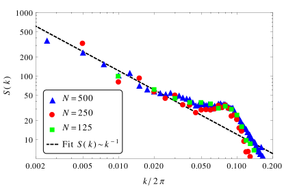
Figure 5: (log-log scale) Numerically calculated PSD of the surfaces at time $t=10^{4}$ produced by (2) with parameter $\alpha=0$ for system sizes (in lattice units) $N=500$ (blue triangles), $N=250$ (red filled circles) and $N=125$ (green squares). The black dashed line represents power-law fit with exponent $\gamma=1.003$.

V.1 Surface spectra

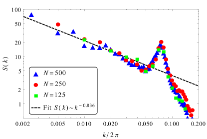
Figure 6: (log-log scale) Numerically calculated PSD of the surfaces at time $t=10^{4}$ produced by (2) with parameter $\alpha=1$ for system sizes (in lattice units) $N=500$ (blue triangles), $N=250$ (red filled circles) and $N=125$ (green squares). The black dashed line represents power-law fit with exponent $\gamma=0.836$.

Since the equation (2) is isotropic, the direction of the wave vector $\boldsymbol{k}$ does not matter in statistical description of height variations, and in spectral analysis of the surface patterns, the wave number $k=|\boldsymbol{k}|$ is sufficient to describe the occurring spatial modes. We can therefore analyze one-dimensional surface spectra $S(k)$, defined in (14).

We calculate the one-dimensional surface spectrum $S(k)$ that depends only on the wave number $k$ using the Wiener-Khinchin theorem which states that the power-spectral density can be obtained from the Fourier transform of the autocorrelation function. Although the height correlation function $C(r)$ (8) depends only on the absolute value $r$ of the shift $\boldsymbol{r}$, it is nevertheless a two-dimensional autocorrelation function of the surface $h(\boldsymbol{r})$. Thus, by applying the two-dimensional Fourier transform on the height correlation function (8), we get the two-dimensional PSD (11) from which we calculate the one-dimensional PSD $S(k)$ using (14).

The numerically calculated height correlation function for an isotropic surface $h(\boldsymbol{r})$ has been defined in (8):

$$C(r)=\Big{\langle}\big{\langle}h_{c}(\boldsymbol{r^{\prime}})\,h_{c}(\boldsymbol{r^{\prime}}+\boldsymbol{r})\big{\rangle}_{\boldsymbol{r^{\prime}}}\Big{\rangle}_{|\boldsymbol{r}|=r}\,.$$

Here, as before, $h_{c}(\boldsymbol{r})=h(\boldsymbol{r})-\bar{h}$ is the surface height with its average value subtracted, the so-called ’centered’ surface profile. The two-dimensional PSD $S_{\boldsymbol{k}}$ is calculated according to (11) with (10):

$$S_{\boldsymbol{k}}=\frac{1}{L^{2}}\int\mathrm{d}^{2}\boldsymbol{r}^{\prime}\,\int\mathrm{d}^{2}\boldsymbol{r}^{\prime\prime}\,h_{c}(\boldsymbol{r}^{\prime})\,h_{c}(\boldsymbol{r}^{\prime\prime})\mathrm{e}^{-\mathrm{i}\boldsymbol{k}\cdot(\boldsymbol{r}^{\prime\prime}-\boldsymbol{r}^{\prime})}\,.$$ (31)

By changing the variable $\boldsymbol{r}^{\prime\prime}\rightarrow\boldsymbol{r}^{\prime}+\boldsymbol{r}$ and switching the order of integration, we get

$$S_{\boldsymbol{k}}=\int\mathrm{d}^{2}\boldsymbol{r}\,\mathrm{e}^{-\mathrm{i}\boldsymbol{k}\cdot\boldsymbol{r}}\frac{1}{L^{2}}\int\mathrm{d}^{2}\boldsymbol{r}^{\prime}\,h_{c}(\boldsymbol{r}^{\prime})\,h_{c}(\boldsymbol{r}^{\prime}+\boldsymbol{r})\,,$$ (32)

where, according to (7),

$$\frac{1}{L^{2}}\int\mathrm{d}^{2}\boldsymbol{r}^{\prime}\,h_{c}(\boldsymbol{r}^{\prime})\,h_{c}(\boldsymbol{r}^{\prime}+\boldsymbol{r})\equiv\big{\langle}h_{c}(\boldsymbol{r^{\prime}})\,h_{c}(\boldsymbol{r^{\prime}}+\boldsymbol{r})\big{\rangle}_{\boldsymbol{r^{\prime}}}=C(\boldsymbol{r})$$ (33)

is the height correlation function of the surface $h(\boldsymbol{r})$.

Since the surfaces $h(\boldsymbol{r})$ generated by (2) are statistically isotropic, the correlation function (33) effectively depends only on $r=|\boldsymbol{r}|$ and can be denoted by $C(r)$. Using this, expressing the two-dimensional integration in (32) over $\boldsymbol{r}$ in the polar coordinates $\boldsymbol{r}=(r,\phi)$ and integrating over the angular part, we get

$$S_{\boldsymbol{k}}=\int\mathrm{d}r\,r\,C(r)\,\int_{0}^{2\pi}\!\mathrm{d}\phi\,\mathrm{e}^{\mathrm{i}kr\cos\phi}\,.$$ (34)

Substituting this into (13) gives the one-dimensional PSD of the surface:

$$S(k)=k\,2\pi\,\int\!\mathrm{d}r\,r\,C(r)\,J_{0}(kr)\,,$$ (35)

Here $J_{0}(kr)$ is the Bessel function of the 1st kind:

$$J_{0}(kr)=\frac{1}{2\pi}\int_{0}^{2\pi}\!\mathrm{d}\phi\,\mathrm{e}^{\mathrm{i}kr\cos\phi}\,.$$ (36)

Figures 5 and 6 show the calculated surface spectra of the surfaces generated by (2) with parameter values $\alpha=0$ (the KSE case) and $\alpha=1$, respectively. In each figure, the spectra for systems of sizes (in lattice units) $N=125$, $N=250$ and $N=500$ are shown. Each spectrum is obtained by averaging over 6 different realizations. The figures confirm the above assumption that increasing the system size does not change the small scale structures, since the spectra at large values of $k$ coincide. The appearance of low wave number modes at larger system sizes and the approximate power-law behavior of the spectrum $S(k)$ can also be seen.

Of course, for larger systems, the numerical calculation of the two-dimensional autocorrelation function (7) and surface spectrum (35) directly can take a very long time. Therefore, the possibility to obtain $S(k)$ from scaling of the surface roughness is very useful.

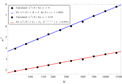
Figure 7: (log-linear scale) Black symbols: numerical results for surfaces evolving according to (2) with $\alpha=0$ (filled circles) and $\alpha=0.25$ (filled squares). Time averaged square of the surface roughness $w^{2}$ plotted as a function of the system size $N$ (in lattice units). Lines: fits of the results for $\alpha=0$ (blue line) and $\alpha=0.25$ (red line) by (23) and (27) respectively, corresponding to the scaling surface spectrum (20). Resulting fit parameters for $\alpha=0.0$: $B=-1.0935$, $C=1.224$; for $\alpha=0.25$: $\gamma=0.991$, $C_{1}=67.770$, $C_{2}=68.284$ .

V.2 Scaling of the surface roughness

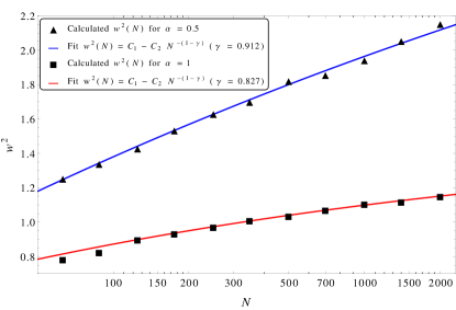
Figure 8: (log-linear scale) Black symbols: numerical results for surfaces evolving according to (2) with $\alpha=0.5$ (filled triangles) and $\alpha=1.0$ (filled squares).Time averaged square of the surface roughness $w^{2}$ plotted as a function of the system size $N$ (in lattice units). Lines: fits of the results for $\alpha=0.5$ (blue line) and $\alpha=1.0$ (red line) by (27) corresponding to the scaling surface spectrum (20). Resulting fit parameters for $\alpha=0.5$: $\gamma=0.912$, $C_{1}=4.554$, $C_{2}=4.768$; for $\alpha=1.0$: $\gamma=0.827$, $C_{1}=1.563$, $C_{2}=1.532$ .

We have investigated the dependence of this saturated surface roughness on the size of the model system for different values of the parameter $\alpha$ in (2). We investigated how the square of $w$ estimated by (6) depends on the system size $N$ (in lattice units) for sizes $N=63$, $N=88$, $N=125$, $N=175$, $N=250$, $N=350$, $N=500$, $N=700$, $N=1000$, $N=1400$, $N=2000$. The results are shown in Fig. 7 for $\alpha=0$ and $\alpha=0.25$, Fig. 8 for $\alpha=0.5$ and $\alpha=1$.

For $\alpha=0$ (the KSE case), the scaling exponent (as introduced in (20)) $\gamma=1$ fits the results best. Thus the dependence of $w^{2}$ on $N$ can be approximated by (23) and the results should form a straight line in the log-linear plot, and, indeed they do as can be seen in Fig. 7 (filled black circles). The blue line in Fig. 7 fitted to data for sizes from $N=88$ to $N=1400$.

For $\alpha=0.25$, the scaling exponent $\gamma\approx 0.991$ fits the results best and the dependence of $w^{2}$ on $N$ can be approximated by (27). Fig. 7 shows the calculated results (filled black rectangles). There seems to be a good agreement between the data and the fitting curve which is fitted to data for sizes from $N=125$ to $N=1400$ (red line in Fig. 7).

The results for $\alpha=0.5$ and $\alpha=1$ give scaling exponents are $\gamma\approx 0.912$ and $\gamma\approx 0.827$, respectively, and the dependence of $w^{2}$ on $N$ can be approximated by (27). Fig. 8 shows the calculated results (black triangles for $\alpha=0.5$ and black rectangles $\alpha=1$) together with their respective fits (blue and red lines in Fig. 8) .

VI Summary and discussion

The generalized Kuramoto-Sivashinsky equation (2) produces surfaces with disordered cellular patterns (Figs. 2, 3 and 4). The size of the average size of a cell depends on equation parameter $\alpha$ and constitutes a definite scale in the surface pattern (see the peaks on the correlation functions in 2). However, in larger systems, the long-range height variations of different character become apparent (Figs. 3 and 4). We investigate these long-range height variations for several values of parameter $\alpha$ by calculating the corresponding scaling relations of the surface roughness.

The square of the surface roughness $w$ (4) which is by definition equal to the variance of the surface height $h(\boldsymbol{r},t)$, $w^{2}\equiv\sigma^{2}_{h}$, can also be expressed as an integral (15) of the one-dimensional power spectral density $S(k)$, given in (14), of the surface over all wave numbers $k$. Since the finite size $L=N\Delta x$ of the system and the discretization step $\Delta x$ in numerical simulations define the approximate lower and upper cut-off values (LABEL:eq:minmax_wavenumber) for the possible wave numbers, the estimated value of $w^{2}$ (19) depends on the system size. As indicated by the surface spectra in Figs. 5 and 6, for systems of increasing size, the small-scale patterns (corresponding to higher wave numbers $k$) remain statistically the same, and, additionally, new lower wave number modes arise in larger systems. Therefore by increasing the size of the system, from the corresponding change in the calculated value of $w^{2}$ (19), the shape of the spatial power spectrum $S(k)$ can be extracted.

If the behavior of $S(k)$ for small wave numbers $k$ (say when $k<k_{\mathrm{s}}$, for some $k_{\mathrm{s}}$) follows the inverse power-law (20), $S(k)\propto k^{-\gamma}$, with $\gamma>0$, this indicates that long-range, scale-free height variations are present. There can be qualitatively distinct cases for different values of the exponent $\gamma$. If $\gamma=1$, then we get the scaling relation (23) which implies that $w$ will grow indefinitely as the system size goes to infinity. If, on the other hand, $\gamma<1$, then we get the scaling relation (27), therefore $w$ will approach finite value (30) as the system size goes to infinity.

For the surfaces generated by numerical simulations of the generalized isotropic Kuramoto-Sivashinsky equation (2), we indeed see the indications that the spatial power spectral density $S(k)$ follows a power-law (20), since the theoretically calculated scaling relations (23) and (27) fit the numerically established scaling of $w^{2}$ well (see Figs. 7 and 8). For the Kuramoto-Sivashinsky equation (1), we get the spectral exponent $\gamma=1$ and the scaling relation (23). For parameter values $\alpha>0$ the scaling exponent $\gamma$ decreases resulting in the scaling relation (27) giving the surfaces of finite roughness as the size of the system goes to infinity, and thus showing that the generalized Kuramoto-Sivashinsky equation (2) with $\alpha>0$ does not belong to the same universality class as the KSE (1).

References

- (1) G. I. Sivashinsky, Acta Astronautica 6, 569 (1979)
- (2) Y. Kuramoto, T. Tsuzuki, Prog. Theor. Phys. 55, 356 (1976)
- (3) I. Procaccia, M. H. Jensen, V. S. L’vov, K. Sneppen, R. Zeitak, Phys. Rev. A 46, 3220 (1992)
- (4) C. Jayaprakash, F. Hayot, R. Pandit, Phys. Rev. Lett. 71, 12 (1993)
- (5) M. Paniconi, K. R. Elder, Phys. Rev. E 56, 2713 (1997)
- (6) M. Rost, J. Krug, Phys. Rev. Lett. 75, 3894 (1995)
- (7) K. B. Lauritsen, R. Cuerno, H. A. Makse, Phys. Rev. E 54, 3577 (1996)
- (8) M. Raible, S. G. Mayr, S. J. Linz, M. Moske, P. Haenggi, K. Samwer, Europhys. Lett. 50, 61 (2000).
- (9) M. Raible, S. J. Linz, P. Haenggi, Phys. Rev. E 64, 031506 (2001).
- (10) R. Gago, R.Vasquez, O. Plantevin, J. A. Sanchez-Garcia, M. Varela, M. C. Ballesteros, J. M. Albella, T. H. Metzger, Phys. Rev. B 73, 155414 (2006).
- (11) R. Cuerno, M. Castro, J. Munoz-Garcia, R. Gago, L. Vasquez, Nucl. Instrum. Methods Phys. Res. B 269, 894 (2011).
- (12) M. Raible, S. J. Linz, P. Haenggi, Acta Physica Polonica B 33, 1049 (2002)
- (13) A.-L. Barabasi, H. E. Stanley, Fractal concepts in surface growth (Cambridge Univ. Press, Cambridge, 1995).
- (14) G. Palasantzas, Phys. Rev. B 48, 14472 (1993)