Local Exponential Methods: a domain decomposition approach to exponential time integration of PDEs

Abstract

A local approach to the time integration of PDEs by exponential methods is proposed, motivated by theoretical estimates by A.Iserles on the decay of off-diagonal terms in the exponentials of sparse matrices. An overlapping domain decomposition technique is outlined, that allows to replace the computation of a global exponential matrix by a number of independent and easily parallelizable local problems. Advantages and potential problems of the proposed technique are discussed. Numerical experiments on simple, yet relevant model problems show that the resulting method allows to increase computational efficiency with respect to standard implementations of exponential methods.

MOX – Modelling and Scientific Computing
Dipartimento di Matematica, Politecnico di Milano
Via Bonardi 9, 20133 Milano, Italy
luca.bonaventura@polimi.it

Keywords: Exponential methods, sparse matrices, stiff partial differential equations, semi-implicit methods, domain decomposition methods.

AMS Subject Classification: 65L04, 65M08, 65M20, 65Z05, 86A10

1 Introduction

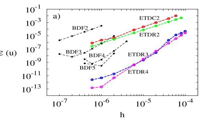
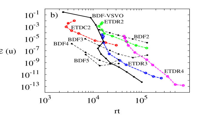
(a) (b)

Figure 1: Errors as a function of time step (a) and computational cost (b) for various IMEX and exponential methods. Reproduced from [12] with the consent of the authors.

The application of exponential time integration methods (EM) to the time discretization of partial differential equations has been the focus of increasing attention over the last two decades. A recent review of these methods is provided e.g. in [15]. EM allow to eliminate almost entirely the time discretization error in the linear case and to reduce it substantially in many nonlinear cases. EM possess stability properties that make them competitive with standard stiff solvers. Furthermore, when wave propagation problems are considered, they also allow to represent faithfully even the fastest linear waves, which are usually damped and distorted by conventional implicit and semi-implicit techniques. After the seminal papers [11], [21], various kinds of exponential methods have been employed by a number of authors in conjunction with different time discretization techniques, see e.g. [1], [6], [12], [18], [19], [22]. In [12], an extensive comparison between IMEX and exponential methods has been carried out. Both kinds of time discretizations have been coupled to a spectral spatial discretization meant for applications to mantle convection problems, but also very similar to numerical techniques widely used in numerical weather prediction and climate modelling. One of the conclusions of this work is highlighted by the graphs in figure 1, that are representative of a large number of numerical simulations carried out in that paper.

While superior in terms of the accuracy achieved when using large time steps, exponential methods appear much more expensive per time step than IMEX methods. Numerical experiments carried out by the author with semi-implicit methids employed in atmospheric modelling point to the same conclusions. The high computational cost is due to the effort in computing the matrix exponential by the Krylov space techniques of [21]. Numerical experiments carried out with other approaches for the exponential matrix computation, such as the Leja points interpolation employed in [19], do not seem to improve things substantially in this respect.

These results motivate the quest for a more economical approach to the computation of the exponentials of sparse matrices typically arising in the space discretization of PDEs. This sparsity corresponds to an effectively finite domain of dependence for the solution of both hyperbolic and parabolic problems. This locality in space of the exact solution of the PDE makes it appear illogical that the exact computation of the spatially discretized solution should be a global operation, involving all the degrees of freedom of the problem, rather than only those that are close to each other in physical space. Such a heuristic consideration has a rigorous counterpart in the results proven in [16] by A.Iserles on the decay of off-diagonal terms in the exponentials of sparse matrices. The bounds proven in [16] imply that, given a sparse matrix ${\bf A}$ representing the spatial discretization of a local, linear differential operator and a vector ${\bf x}$ representing the discrete degrees of freedom, for any node $i$ the contribution to $({\exp({\bf A}\Delta t)}{\bf x})_{i}$ of nodes $j$ that are sufficiently far from $i$ in physical space is small. How far and how small will obviously depend on the time step $\Delta t$ and on the speed of propagation of information in the PDE discretized by ${\bf A}.$ Extensions of this result have been proposed more recently in [3], [4], [5].

Motivated by these considerations, an overlapping domain decomposition technique is proposed here, that allows to replace the computation of a global exponential matrix by a number of independent local matrices. The obvious advantage of such a Local Exponential Method (LEM) is that each local problem can be solved independently in parallel, thus increasing the scalability of the resulting time discretization technique. Furthermore, if the number of degrees of freedom associated to each local domain is small enough, the local exponential matrices can be computed by Padé approximation combined with scaling and squaring (see e.g. [20] for a review of numerical methods for the computation of matrix exponentials) and can be actually stored in memory, thus bypassing the problems that result from having to compute the action $({\exp({\bf A}\Delta t)}{\bf x})$ rather than the exponential matrix itself. The main drawback of the proposed approach is that, in each of the local problems, some of the nodes also associated to other subdomains are updated just for the sake of providing a buffer zone that makes the domain under consideration only marginally affected by the far field. For hyperbolic problems, the size of this buffer zone depends on the Courant number, which clearly implies that the method becomes increasingly inefficient in the limit of very large Courant numbers. However, some situations exist in which the proposed approach seems competitive in spite of this limitation. In some linear problems relevant for many applications, such as the Schrödinger equation, being able to store the local matrices required for approximation of the exponential matrix can significantly reduce the computational cost. In high order finite element methods, high Courant numbers arise easily due to the large number of degrees of freedom per element (see e.g. the related discussion and proposals in [23]), so that a technique that enables to run at Courant numbers of the order of the polynomial degree employed with a more local approach could turn out to be useful. Furthermore, in many environmental applications, such as numerical weather prediction and ocean modelling, strongly anisotropic meshes are employed, with a vertical resolution that is often two or three orders of magnitude smaller than the horizontal one. This results in high vertical Courant numbers, that are often addressed by directional splitting methods. The present approach would allow to achieve the same goal by employing a horizontal domain decomposition approach with minimal overlap among subdomains, such as almost universally used for parallelization of this kind of models, while at the same time avoiding ad hoc solutions that rely on splitting and providing an efficient and robust way to solve the corresponding fluid dynamics equations.

In section 2, the key results of [16] are reviewed and applied to the spatial discretization of a simple model problem. In section 3, an overlapping domain decomposition approach to exponential time integration methods is outlined and the potential advantages and problems of the proposed technique are discussed. In section 4, some numerical results on simple one and two dimensional problems are reported, that show that the proposed approach is able to attain the same accuracy level as either standard time discretization methods or global implementations of exponential integrators. Some conclusions and perspectives for future work are outlined in section 5.

2 Exponentials of sparse matrices and PDEs

The key theoretical result for the development proposed in this paper has been proven in [16] and will be briefly summarized here.

Theorem 1

Consider a sparse, $s-$banded matrix ${\bf A}=(a_{i,j})$ and assume that its non zero entries are bounded by $\max_{i,j}|a_{i,j}|\leq\rho.$ Denoting then $\exp({\bf A})=(e_{i,j})$ one has

$$|e_{i,j}| \leq \Big{(}\frac{\rho s}{|i-j|}\Big{)}^{\frac{|i-j|}{s}}\Big{[}{\rm e}^{\frac{|i-j|}{s}}-\sum_{k=0}^{|i-j|-1}\frac{(|i-j/s|)^{k}}{k!}\Big{]}$$ (1)

$$\approx \Big{(}\frac{\rho s}{|i-j|}\Big{)}^{\frac{|i-j|}{s}}\frac{(|i-j|/s)^{|i-j|}}{|i-j|!}$$

Some remarks on this result are necessary before proceeding to the application to spatial discretizations of PDEs. Firstly, in many exponential matrix it is necessary or convenient to use, rather than the exponential itself, the so called $\phi-$ functions, defined recursively as

$$\phi_{k}(z)=\frac{\exp{(z)}-\sum_{l=0}^{k}z^{l}/l!}{z^{k}}.$$

The function $\phi_{1}$ will be simply denoted as $\phi$ in the following. Although theorem 1 as stated in [16] refers strictly speaking to the exponential function only, the bounds given in the same paper on the size of the entries of powers ${\bf A}^{m}$ could be employed to derive similar decay estimates for the off diagonal terms of $\phi_{k}({\bf A}).$ Here, we do not pursue the rigorous extension of 1 to exponential related functions. Furthermore, theorem 1 is proven strictly speaking only for matrices with limited bandwith, while in spatial discretizations of multidimensional PDEs more complex sparsity patterns easily arise. Here, it will be again assumed heuristically that analogous estimates can be provided also in these more relevant cases, although it is clear that deriving general proofs may be far from easy. Numerical results reported in section 4 seem to provide heuristic evidence that the required generalizations of 1 hold.

Given this caveat, it is possible to argue that theorem 1 has important implications for the application of exponential methods to the time discretization of PDEs. We will consider as a model problem the linear advection diffusion equation and its associated initial and boundary value problem on the spatial domain ${\Omega}$

$$\frac{\partial c}{\partial t}=-{\bf a}(x)\cdot\nabla c+\nu(x)\Delta c,\ \ \ \ t\in[0,T]\ \ \ x\in\Omega$$

$$c(x,0)=c_{0}(x)$$ (2)

with appropriate boundary conditions (taken here for simplicity to be time independent) defined by the linear operator ${\cal B}c=g$ at $\partial\Omega.$ Here ${\bf a}(x)$ denotes the velocity field and $\nu(x)$ the non negative diffusivity. Denote then by ${\cal M}$ a computational mesh with minimum element size $\Delta x$ for the approximation of (2) by some consistent space discretization technique. Denote by ${\bf u}$ the vector of the associated discrete degrees of freedom and by ${\bf A}$ the matrix representing the spatial discretization. Problem (2) will then be approximated by

$$\frac{d{\bf u}}{dt}={\bf A}{\bf u}+{\bf g}$$

$${\bf u}(0)={\bf u}_{0},$$ (3)

where now by a slight abuse of notation ${\bf g}$ denotes the non autonomous forcing resulting from the spatial discretization of the boundary conditions ${\cal B}c=g$ and ${\bf u}_{0}$ denotes the approximation of $c_{0}(x)$ in the chosen finite dimensional setting. The solution of problem 3 is given by

$${\bf u}(t)=\exp{({\bf A}t)}{\bf u}_{0}+\int_{0}^{t}\exp{({\bf A}(t-s))}{\bf g}\ ds={\bf u}_{0}+t\phi\big{(}t{\bf A}\big{)}\Big{(}{\bf A}{\bf u}+{\bf g}\Big{)}.$$

It is well known that this formula is the basis of all exponential methods, that in many cases simply reduce to it for linear problems with constant forcing. For any reasonable, consistent spatial discretization, it will follow that the entries of $\Delta t{\bf A}$ will be bounded by

$$\rho=O\Big{(}C+\mu\Big{)},\ \ \ C=\max_{x\in\Omega}|{\bf a}(x)|\frac{\Delta t}{\Delta x}\ \ \ \ \mu=\max_{x\in\Omega}\nu(x)\frac{\Delta t}{\Delta x^{2}},$$

where $C,\mu$ denote, respectively, the maximum Courant number and the stability parameter of standard explicit discretizations of the heat equation.

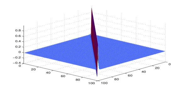
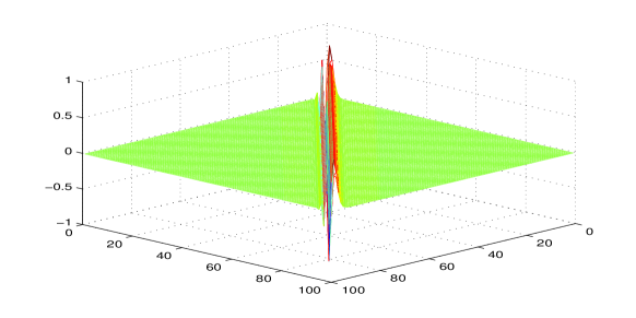
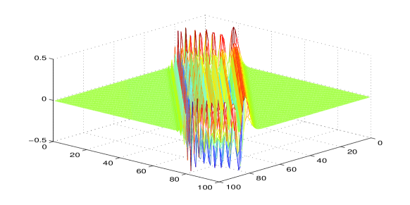
(a) (b) (c)

Figure 2: Visualization of ${\exp}(\Delta t{\bf A})$ in the case of the centered finite difference approximation of advection in 1d at Courant numbers (a) 0.5, (b) 5, (c) 20.

This implies that the degree of sparseness of ${\exp}(\Delta t{\bf A})$ and of the related functions will depend on the magnitude of the usual stability parameters for explicit time discretizations. This can be visualized graphically by considering a simple centered finite difference approximation on a uniform mesh for the one dimensional case with $\mu=0$ with homogeneous Dirichlet boundary conditions. The matrix $\Delta t{\bf A}$ is visualized in figure 2 for Courant numbers $0.5,5,20,$ respectively. Entries away from the diagonal are non zero, but have an absolute value that decays rapidly for bands further away from the diagonal than the Courant number. Even though the diffusion operator has an infinite domain of dependence in the continuous case, a similar pattern is observed for simple discretizations of the diffusive terms. Strategies to obtain optimal bounds for the entries of the exponential are proposed in [16] and the issue of how to estimate rigorously an optimal bound in more general cases is definitely an open one. However, as shown in the practical applications to PDE problems presented in section 4, one can simply rely on the inspection of the standard stability parameters, like the Courant number, to identify the size of the mesh region that is effectively contributing to the change in the solution associated with a given node within one time step. These considerations lead to the idea that the computation of the global exponential matrix required by standard approaches to application of exponential integrators for PDEs can be replaced by the computation of local matrices, associated to the exact solution of the restriction of (3) to appropriate subsets of the computational domain.

3 Local exponential methods: a domain decomposition approach to exponential time integration methods

The theoretical results summarized in the previous section suggest a more local approximation of exponential matrices for time discretization of linear PDEs. One possible approach will be now be introduced and denoted shortly as Local Exponential Method (LEM) in the following. The first step consists in decomposing the mesh in $D$ overlapping regions

$${\cal M}=\bigcup_{i=1}^{D}{\cal M}_{i}\ \ \ {\cal M}_{i}={\cal D}_{i}\cup{\cal B}_{i}.$$

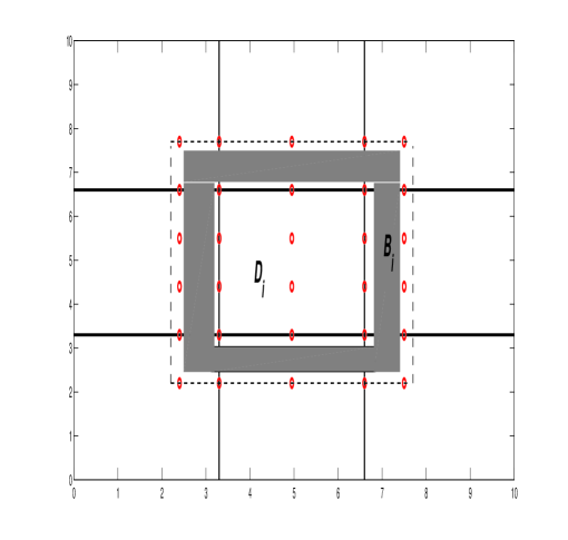
Figure 3: Sketch of a domain ${\cal D}_{i}$ with the corresponding buffer region ${\cal B}_{i}$ highlighted in grey.

Here ${\cal D}_{i}$ denote non overlapping domains, such that ${\cal M}=\bigcup_{i=1}^{D}{\cal D}_{i},$ while ${\cal B}_{i}$ are boundary buffer zones surrounding each ${\cal D}_{i}.$ A visualization of one such region is sketched in figure 3.

Notice that, after the space discretization (3), the mesh is only assumed to include interior nodes, while the effect of boundary conditions is included in the forcing term. One can then denote by ${\bf u}_{{\cal M}_{i}},$ ${\bf u}_{{\cal D}_{i}}$ the set of discrete degrees of freedom associated to ${\cal M}_{i},{\cal D}_{i},$ respectively and by ${\bf A}_{{\cal M}_{i}}$ the restriction of the matrix ${\bf A}$ to the nodes in ${\cal M}_{i}.$ Given these definitions, we now outline the LEM in the case of the simplest exponential method, i.e. the exponential Euler method (see e.g. [15]). The extension to any of the exponential methods described in the literature is immediate. Introduce a discrete set of time levels $t_{n},$ taken for simplicity to be equally spaced and such that $t^{n+1}-t^{n}=\Delta t.$ Then, for each $i=1,\dots,D,$ and $t^{n},$

• consider the local problems restricted to ${\cal M}_{i}$

  $$\frac{d{\bf v}_{{\cal M}_{i}}}{dt}={\bf A}_{{\cal M}_{i}}{\bf v}_{{\cal M}_{i}}+{\bf g}_{{\cal M}_{i}}(t),$$ (4)

  where ${\bf v}_{{\cal M}_{i}}(t^{n})$ is assumed to coincide with ${\bf u}^{n}_{{\cal M}_{i}}$ and ${\bf A}_{{\cal M}_{i}},{\bf g}_{{\cal M}_{i}}(t),$ are modified with respect to the simple restriction of their global counterparts in order to impose Dirichlet boundary conditions along the parts of the boundaries $\partial{\cal B}_{i}$ that belong to some domain ${\cal D}_{j}$ with $j\neq i;$

• compute

  $${\bf v}_{{\cal M}_{i}}^{n+1}={\bf v}_{{\cal M}_{i}}^{n}+\Delta t\phi(\Delta t{\bf A}_{{\cal M}_{i}})\Big{(}{\bf A}_{{\cal M}_{i}}{\bf v}^{n}_{{\cal M}_{i}}+{\bf g}_{{\cal M}_{i}}(t^{n})\Big{)};$$ (5)

• define ${\bf u}_{{\cal D}_{i}}^{n+1}={\bf v}_{{\cal D}_{i}}^{n+1},$ thus overwriting the degrees of freedom belonging to the buffer zones.

It is clear that, if the solution of each local problem (4) is to be a good approximation of the solution of global problem (3), the buffer regions must be chosen in such a way that the contribution to $\phi(\Delta t{\bf A}_{{\cal M}_{i}})$ from nodes $k\notin{\cal M}_{i}$ is negligible. As discussed in the previous section, for discretizations of the model problem (2) it should be sufficient to choose a size that, given a value of $\Delta t,$ is related to the typical stability parameters of explicit time discretizations. In the simple tests described in section 4, on cartesian meshes the size of the buffer regions is taken to be (empirically) related to the maximum between $C$ and $\mu.$

A number of obvious potential advantages of LEM are apparent. First of all, the computation of the local exponential matrices is trivially parallel, thus leading to an algorithm that should scale much better on massively parallel machines than those requiring a global communication step. Furthermore, the size of the exponential matrices to be computed will be smaller, thus implying that, if e.g. Krylov space techniques are employed for their computation, a smaller dimension of the Krylov space would be sufficient for their accurate approximation. Finally, for small enough subdomains ${\cal M}_{i},$ the resulting local matrices could be computed by simpler methods, such as direct Padé approximation (see e.g. [20]), and stored in the local memory. This contrasts with the computation of the action of the exponential matrix that is necessary in standard implementations for large ODE systems deriving from spatial semidiscretization of PDEs. Storage of the local matrices would also allow to to increase the efficiency of methods such as the exponential Rosenbrock methods proposed in [13], by allowing to freeze the Jacobian matrix of the right hand side over a certain number of time steps.

Some disadvantages of the proposed approach are also obvious. The degrees of freedom belonging to the buffer regions only play an auxiliary role and would be updated at least twice (or more, if the corresponding nodes belong to more than two buffer regions). This implies that there is a computational overhead that is proportional to the size of such regions. Considering for simplicity the pure advection problem, this implies that the method is increasingly less efficient in the limit of increasing Courant number, which is exactly the limit in which exponential methods are most advantageous with respect to more standard ones. In which regimes the resulting algorithm could end up in being more efficient than standard ones is not obvious. However, some situations can easily be identified in which the proposed approach seems competitive in spite of this limitation. In high order finite element methods, for example, high Courant numbers arise easily due to the large number of degrees of freedom per element (see e.g. [23]), so that a technique that is able to run at Courant numbers of the order of the polynomial degree employed with a more local approach could turn out to be useful. Furthermore, in many environmental applications, such as numerical weather prediction and ocean modelling, strongly anisotropic meshes are employed, with a vertical resolution that is often two or three orders of magnitude smaller than the horizontal one. This results in high vertical Courant numbers, that are often addressed by directional splitting methods. The present approach would allow to achieve the same goal by employing a horizontal domain decomposition approach with minimal overlap among subdomains, such as almost universally used for parallelization of this kind of models, while at the same time avoiding ad hoc solutions that rely on splitting and providing an efficient and robust way to solve the corresponding fluid dynamics equations. The preliminary numerical results reported in section 4 support the view that an acceptable trade off between locality and efficiency is feasible and motivate further investigation of the application of LEM to fluid dynamics and wave propagation problems. Furthermore, if environmental models with complex physical parameterizations are considered, LEM would provide a completely local approach to include these terms while maintaining high order accuracy in time without extra computational costs. Indeed, if the second order exponential Rosenbrock method is considered, second order accuracy in time would be attainable with a single evaluation of the right hand side, without the need for ad hoc splitting procedures such as those customarily employed in most models of this kind and analysed e.g. in [8], [9], [10].

4 Numerical results

A number of numerical experiments have been carried out with preliminary implementations of the approach outlined in the previous sections. In particular, since the error bounds presented in [16] do not provide a sharp estimate for the error resulting from the proposed domain decomposition approach, the goal of these tests is to assess the effective accuracy of the resulting space-time discretization, as well as to estimate the sensitivity of the results to the choice of the size of the buffer regions. Only simple finite difference and finite volume discretizations have been considered in this work, although it is clear that the results will also depend in general on the chosen spatial discretization. A further goal of these tests is to understand to which extent the proposed method leads to a reduction in computational cost with respect to approaches in which the exponential matrix is computed globally, although, due to the preliminary nature of the implementation, the estimates of the CPU times of each method are to be considered only as rough indications of its computational cost. In all the tests, the exponential Euler-Rosenbrock methods proposed in [14] have been employed, which reduce in the linear case to the exponential Euler method. In the one dimensional tests, the $\phi$ matrix was computed by the scaling and squaring algorithm and Padé approximation. For the linear test cases, the $\phi$ matrices associated to each subdomain were computed only at the first time step. In the nonlinear test cases, the Jacobian of the ODE system and the corresponding $\phi$ matrices were computed at the first time step and later kept constant for a number of time steps chosen empirically for each case.

4.1 One-dimensional, linear tests

In a first set of numerical tests, the simple one-dimensional, constant coefficient, linear advection diffusion equation

$$\frac{\partial{c}}{\partial t}=-u\frac{\partial{c}}{\partial x}+\nu\frac{\partial^{2}c}{\partial x^{2}}$$ (6)

has been considered on a time interval at $[0,T]$ and on an spatial interval $[0,L]$ with periodic boundary conditions, along with the one-dimensional Schrödinger equation with harmonic potential

$$\frac{\partial c}{\partial t}=\frac{i}{2}\frac{\partial^{2}c}{\partial x^{2}}-i\frac{\kappa}{2}x^{2}c$$ (7)

with periodic boundary conditions on an interval $[-L/2,L/2]$ and $\kappa=10.$ In both cases, the differential operators have been approximated by simple centered finite difference formulae and a Gaussian initial datum was considered.

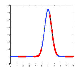
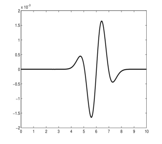
(a) (b)

Figure 4: Approximation of the advection diffusion equation at $T=3$ by local exponential method applied over 8 subdomains with sufficiently large overlap: (a) reference solution by Fourier method and separation of variables (black line) and numerical solution (blue or red symbols depending on the subdomain); (b) absolute error.

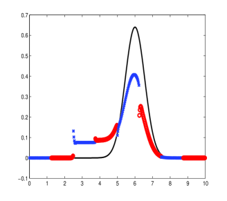
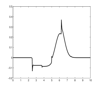
(a) (b)

Figure 5: Approximation of the advection diffusion equation at $T=3$ by local exponential method applied over 8 subdomains with insufficiently large overlap: (a) reference solution by Fourier method and separation of variables (black line) and numerical solution (blue or red symbols depending on the subdomain); (b) absolute error.

The first goal of the tests is to show that the approach outlined in section 3 does not lead in practice to any loss of accuracy, as long as a sufficiently large overlap is allowed among neighboring subdomains. Numerical experiments confirm that this is indeed the case. As an example, the numerical solution of (6) computed at $T=3$ time units on a domain of size $L=10$ is displayed in figure 4. The discretization employs 400 grid points subdivided into 8 identical subdomains. The simulation was run with $u,\nu,$ and $\Delta t$ values resulting in the values $C\approx 4,$ $\mu\approx 4.8$ for the usual stability parameters and using buffer regions of size 18 grid points on each side of the subdomains considered. It can be seen that the error structure is regular in space and only depends on the spatial derivatives of the solution, as expected in the case of a generic time discretizations. As in the case of the standard exponential method, the dominant error component is due to the spatial discretization error, as it can be seen by comparing the result with a reference solution of the ODE system associated to the same spatial semi-discretization obtained by a high order accurate reference solver with automatic error estimation and error tolerance of the order $10^{-9}.$ The errors obtained by the local exponential method are, as long as the buffer region is sufficiently large, essentially identical to those of the standard exponential method applied by global computation of the exponential matrix. On the other hand, the error obviously increases as the buffer region size is reduced, ultimately leading to totally erroneous solutions where the subdomain imprinting is clearly visible, see as an example the same solution displayed before as computed with a buffer region of size 5 gridpoints in figure 5.

In order to assess the potential of the proposed domain decomposition technique for reduction of the computational cost associated to exponential methods, the same test was repeated progressively increasing the time step and changing the number of subdomains employed. The results are displayed in table 1, where $D$ denotes the number of subdomains employed and $B$ the number of grid points in the buffer regions. The case $C=8,B=20,D=20$ was not run, since the subdomains would have been of the same size as the buffer regions. In all the tests reported in this table, relative errors of approximately $3\times 10^{-3}$ were obtained, which is approximately of the same magnitude as that obtained on the same test by an explicit Runge Kutta method of order 3 run at $C=0.5,\mu=0.5.$

	$D=1$	$D=2$	$D=4$	$D=5$	$D=10$	$D=20$
$C=1,\mu=1,B=8$	1.85	0.59	0.39	0.47	0.75	1.35
$C=2,\mu=2,B=12$	2.85	0.65	0.28	0.30	0.65	0.78
$C=4,\mu=4,B=15$	2.89	1.64	0.23	0.77	0.31	0.54
$C=8,\mu=8,B=20$	3.79	1.00	0.23	0.23	0.25	-

Table 1: CPU times (in seconds) for LEM runs in the linear advection diffusion test case, as a function of the time step, the number $D$ of subdomains employed and the number of grid points $B$ in the buffer regions.

Firstly, it must be observed that the CPU times of the standard exponential methods are increasing as a function of the stability parameters. This may seem a paradox, since in this case only one matrix function evaluation is necessary for each run. However, the number of scaling and squaring steps to be performed in the computation of the $\phi$ matrix increases as $\Delta t$ increases, thus leading to a larger computational cost in the case of longer time steps. The potential of the LEM approach is apparent, since CPU times are reduced by a factor ranging from $5$ to $20.$ The domain decomposition approach also seems competitive with standard implicit methods, since for example the CPU time for a Crank Nicolson method run at $C=4,\mu=4$ performed without repeating the matrix evaluation is around $0.3$ seconds, but with an error that is approximately one order of magnitude larger. On the other hand, in this simple case the fastest LEM runs still take approximately 5 times longer than an explicit Runge Kutta method of order 3 run at $C=0.5,\mu=0.5.$

In the case of the Schrödinger equation, a numerical solution of (7) was computed at $T=1$ time units on a domain of size $L=10$ on a mesh with 400 grid points and a reference solution was computed discretizing in space by a pseudospectral Fourier approach and employing a high order accurate reference ODE solver with automatic error estimation and error tolerance of the order $10^{-9}$ for the time discretization. The results are displayed in table 2. In all the tests reported in this table, relative errors of approximately $6\times 10^{-4}$ were obtained, which is approximately of the same magnitude as that obtained on the same test by an explicit Runge Kutta method of order 3 run at $\mu=0.2.$ Notice that, in this case, also the oscillatory term $i\kappa x^{2}/2$ has a major impact on stability of explicit methods.

	$D=1$	$D=2$	$D=4$	$D=5$	$D=10$
$\mu=2,B=20$	8.21	5.74	4.56	4.45	6.32
$\mu=4,B=25$	12.83	3.92	2.65	3.08	5.04

Table 2: CPU times (in seconds) for LEM runs in the Schrödinger equation test case, as a function of the time step, the number $D$ of subdomains employed and the number of grid points $B$ in the buffer regions.

It can be seen that, in this case, the cost reduction is not as impressive as in the case of the advection diffusion problem. However, it is to be remarked that, for this test, the standard implementation of the exponential methods leads to CPU times that are of the same order of that required by the Crank Nicolson method run with the same time step. Furthermore, the fastest LEM runs take in this case approximately 5 times less than an explicit Runge Kutta method of order 3 run at $\mu=0.2.$ As a result, the LEM approach appears to be competitive both with standard explicit and implicit methods in the case of the one dimensional Schrödinger equation.

4.2 One dimensional, nonlinear tests

Several nonlinear tests have also been performed with the proposed discretization approach. As a first nonlinear benchmark, the time discretization of (6) was considered again, with a space discretization given by a second order, monotonized finite volume approach employing a minmod flux limiter. In this case, it is well known (see e.g. [17]) that also the space semi-discretization of a linear advection problem results in a nonlinear ODE system. This model problem is relevant for applications since, in practice, the advection equation is rarely discretized without introducing some analogous monotonization approach. Furthermore, an example of more naturally nonlinear problems, the one-dimensional viscous Burgers equation

$$\frac{\partial{c}}{\partial t}=-\frac{\partial}{\partial x}\left(\frac{c^{2}}{2}\right)+\nu\frac{\partial^{2}c}{\partial x^{2}}$$ (8)

has been considered, whose nonlinearities are typical of computational fluid dynamics problems, along with the nonlinear parabolic equation

$$\frac{\partial{c}}{\partial t}=\frac{\partial^{2}c^{m}}{\partial x^{2}},$$ (9)

for which an exact solution is available (see e.g. [2], [7]), given by

$$u(x,t)=(t+t_{0})^{-k}\left(A^{2}-\frac{k(m-1)|x|^{2}}{2m(t+t_{0})^{2k}}\right)_{+}^{\frac{1}{m-1}}$$ (10)

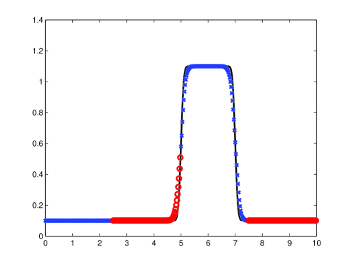
Figure 6: LEM approximation of the solution of the advection diffusion equation discretized in space by a monotonized finite volume method. The solution is shown at $T=3$ as computed over 4 subdomains with sufficiently large overlap: reference solution (black line) and numerical solution (blue or red symbols depending on the subdomain).

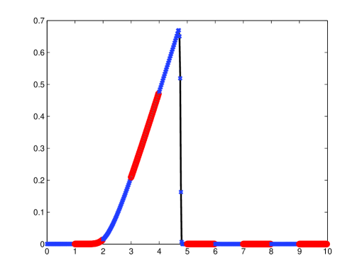
Figure 7: Approximation of the solution of the Burgers equation at $T=6$ by local exponential method applied over 10 subdomains with sufficiently large overlap: reference solution (black line) and numerical solution (blue or red symbols depending on the subdomain).

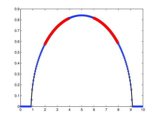
Figure 8: Approximation of the solution of the nonlinear diffusion equation at $T=1$ by local exponential method applied over 5 subdomains with sufficiently large overlap: reference solution (black line) and numerical solution (blue or red symbols depending on the subdomain).

where $t_{0}>0$, $A$ is an arbitrary nonzero constant and $k=1/(m+1).$ A monotonized second order finite volume approach was employed for the spatial discretization also for the Burgers equation, while equation 9 was discretized by simple centered finite differences. In all cases, an interval of size $L=10$ was considered and computational mesh with $400$ control volumes of equal size was employed. Examples of solutions of these equations obtained by LEM discretization employing a third order exponential Rosenbrock method are shown in figures 6, 7, 8, respectively. In the case of the advection diffusion equation, a square wave initial datum was considered, while in the case of the Burgers equation the initial datum was taken to be Gaussian and for equation 9 the initial condition was chosen so as to recover the analytic solution of [2] with $m=3$, $A=1$.

In a first numerical experiment aimed at checking the performance improvements in a purely hyperbolic case, the pure advection equation was considered. CPU times for the LEM discretization with the second order exponential Rosenbrock method are displayed in table 3, while the corresponding times for the third order exponential Rosenbrock method are displayed in table 4. In this test, the final time was taken to be $T=4$ and the Jacobian matrices used by the Rosenbrock exponential methods and the associated $\phi$ matrices were recomputed every 5 time steps. Notice that in this test with non smooth initial datum (and solution), time steps resulting in Courant numbers larger than approximately 1.6 result in violations of monotonicity for the numerical solution. In all these tests, the relative $l_{\infty}$ and $l_{2}$ errors are approximately 0.39 and 0.12, respectively. The error is mostly associated to the spatial discretization error, as it can be seen comparing to solutions obtained by the same spatial discretization coupled to a reference solver with small error tolerance. As a comparison, explicit Runge Kutta methods of order 2 and 3 run yield analogous errors when run at Courant numbers between $C=0.2$ and $C=0.3,$ respectively, with corresponding CPU times approximately 0.8 and 1 seconds. On the other hand, a Crank-Nicolson time discretization run at Courant numbers $C=1$ and $C=1.6,$ yields relative $l_{\infty}$ errors of 0.45 and 0.5 and CPU times of 11.24 and 6.84 seconds, respectively.

	$D=1$	$D=2$	$D=4$	$D=5$	$D=8$	$D=10$
$C=0.5,B=5$	31.7	17.24	13.00	9.72	8.81	9.11
$C=1,B=10$	28.77	8.96	5.59	5.46	5.47	5.48
$C=1.6,B=15$	18.04	5.58	3.90	3.95	3.90	4.26

Table 3: CPU times (in seconds) for LEM runs with second order exponential Rosenbrock method in the advection test case with monotonized finite volume discretization, as a function of the time step, the number $D$ of subdomains employed and the number of grid points $B$ in the buffer regions.

	$D=1$	$D=2$	$D=4$	$D=5$	$D=8$	$D=10$
$C=0.5,B=5$	32.73	15.83	10.53	9.11	9.24	9.66
$C=1,B=10$	15.66	8.21	5.77	5.54	5.13	6.32
$C=1.6,B=15$	9.9	6.59	4.55	4.26	4.42	5.28

Table 4: CPU times (in seconds) for LEM runs with third order exponential Rosenbrock method in the advection test case with monotonized finite volume discretization, as a function of the time step, the number $D$ of subdomains employed and the number of grid points $B$ in the buffer regions.

In the case of the Burgers equation, a viscosity of $\nu=0.05$. A reference solution was computed in this case by the same spatial discretization coupled to a reference solver with small error tolerance. Therefore, in this case only an estimate of the time discretization error of the different methods is available. CPU times for the LEM discretization with the second order exponential Rosenbrock method are displayed in table 5, while the corresponding times for the third order exponential Rosenbrock method are displayed in table 6. In this test, the final time was taken to be $T=5$ and the Jacobian matrices used by the Rosenbrock exponential methods and the associated $\phi$ matrices were recomputed every 5 time steps.

	$D=1$	$D=2$	$D=4$	$D=5$	$D=8$	$D=10$
$C=0.4,\mu=0.8,B=8$	58.26	15.77	11.06	9.06	10.32	9.76
$C=1,\mu=2,B=15$	50.91	11.46	4.70	4.49	4.53	5.03
$C=2,\mu=4,B=20$	36.35	7.93	2.80	3.19	3.29	3.13

Table 5: CPU times (in seconds) for LEM runs with second order exponential Rosenbrock method in the Burgers test case, as a function of the time step, the number $D$ of subdomains employed and the number of grid points $B$ in the buffer regions.

	$D=1$	$D=2$	$D=4$	$D=5$	$D=8$	$D=10$
$C=0.4,\mu=0.8,B=5$	25.89	13.46	10.63	10.30	10.09	10.42
$C=1,\mu=2,B=15$	30.07	9.02	4.70	4.72	4.78	5.49
$C=2,\mu=4,B=20$	26.77	6.57	2.87	3.24	3.05	3.13

Table 6: CPU times (in seconds) for LEM runs with third order exponential Rosenbrock method in the Burgers test case, as a function of the time step, the number $D$ of subdomains employed and the number of grid points $B$ in the buffer regions.

4.3 Two dimensional tests

In a preliminary assessment of the performance of the proposed method in two dimensions, an advection diffusion problem was again considered, formulated as

$$\frac{\partial c}{\partial t}=-\nabla\cdot({\bf a}(x)c)+\nu\Delta c,\ \ \ \ t\in[0,T]\ \ \ x\in\Omega$$

$$c(x,0)=c_{0}(x)$$ (11)

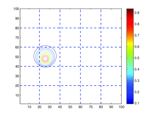
Figure 9: Approximation of the solution of the advection diffusion equation in a solid body rotation test. The subdomains employed are indicated by dashed blue lines.

where ${\bf a}(x)$ is a divergence free velocity field. As in sections 4.1 and 4.2, either simple centered finite differences or a monotonized finite volume method were employed for spatial discretization. For the approximation of the $\phi$ functions, the Krylov space method of [21] was employed for the reference implementation of the standard exponential method. In the case of LEM, the action of the local $\phi$ functions was computed, in the present preliminary implementation, also by the Krylov space method. A an example of result in this test case is displayed in figure 9, where 25 subdomains have been employed. Concerning a first quantitative assessment, the errors of the second order exponential Rosenbrock method run at Courant number 7 where analogous to those obtained by an explicit Runge Kutta method of order 4.

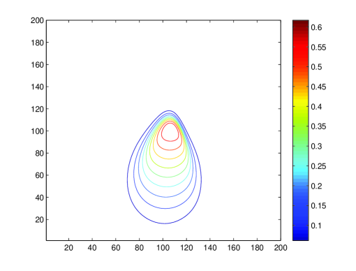
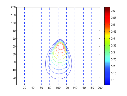
(a) (b)

Figure 10: Approximation of the solution of the two-dimensional viscous Burgers equation, computed (a) by a single domain approach (b) by a multidomain approach. The subdomains employed are indicated by dashed blue lines.

A nonlinear example was also considered, given by a two dimensional extension of a nonlinear Burgers equation. This problem was solved on an anisotropic finite volume mesh with vertical spacing much smaller than the horizontal one. A result obtained by the second order exponential Rosenbrock method, run at Courant number 6 in the vertical direction and Courant number below one in the horizontal direction, is shown in figure 10. In this case, a column-wise domain decomposition was employed, which allowed to minimize the overlap in the horizontal direction.

5 Conclusions and future work

An overlapping domain decomposition technique has been proposed, motivated by the results of A.Iserles [16], that allows to approximate the global matrices employed in exponential time integration methods for time dependent PDEs by smaller ones that are related to the spatial subdomains in which the mesh is decomposed. The resulting Local Exponential Method (LEM) requires only the solution of local problems that can be easily parallelized, thus increasing the scalability of the resulting time discretization technique. Furthermore, if the number of degrees of freedom associated to each local subdomain is small enough, the local exponential matrix can be computed by simple Padé approximation and can be stored, thus bypassing the problems that result from having to compute the action rather than the exponential matrix itself. The main drawback of the proposed approach is that, in each of the local problems, a portion of the local degrees of freedom is only playing an auxiliary role. As a result, their update is recomputed multiple times, so that there is an significant overhead with respect to a standard time discretization, which is proportional to the size of the buffer regions. In spite of this overlap, preliminary numerical simulations show a significant reduction in computational cost with respect to standard exponential methods.

The results obtained so far appear to justify the further investigation of this approach in the framework of more complex spatial discretizations and model problems. Several situations exist in which the proposed approach could be useful in spite of its limitation. In high order finite element methods, high Courant numbers arise easily due to the large number of degrees of freedom per element, so that a technique that enables to run at Courant numbers of the order of the polynomial degree employed with a more local approach should be competitive. Furthermore, in many environmental applications, such as numerical weather prediction and ocean modelling, strongly anisotropic meshes are employed, with a vertical resolution that is often two or three orders of magnitude smaller than the horizontal one. This results in high vertical Courant numbers, that are often addressed by directional splitting methods. The present approach would allow to achieve the same goal by employing a horizontal domain decomposition approach with minimal overlap among subdomains, such as almost universally used for parallelization of this kind of models, while at the same time avoiding ad hoc solutions that rely on splitting and providing an efficient and robust way to solve the corresponding fluid dynamics equations. This would be especially useful for models including complex physical parameterizations. Indeed, LEM would provide a completely local approach to account for these terms while maintaining high order accuracy in time without extra computational costs. For this reason, the application of LEM to high order adaptive DG discretizations will be studied, in order to compare their accuracy and efficiency to that of the semi-implicit, semi-Lagrangian techniques introduced e.g. in [23].

References

- [1] R. Archibald, K.J. Evans, J. Drake, and J.B. White III. Multiwavelet Discontinuous Galerkin-Accelerated Exact Linear Part (elp) Method for the Shallow Water Equations on the Cubed Sphere. Monthly Weather Review, 139:457–473, 2011.
- [2] G. I. Barenblatt. On self-similar motions of a compressible fluid in a porous medium. Akad. Nauk SSSR. Prikl. Mat. Meh, 16(6):79–6, 1952.
- [3] M. Benzi and P. Boito. Decay properties for functions of matrices over -algebras. Linear Algebra and its Applications, 456:174–198, 2014.
- [4] M. Benzi and V. Simoncini. Approximation of functions of large matrices with Kronecker structure. Technical Report 1503.02615, arXiv, 2015.
- [5] M. Benzi and V. Simoncini. Decay bounds for functions of matrices with banded or Kronecker structure. Technical Report 1501.07376, arXiv, 2015.
- [6] G. Beylkin, J. M. Keiser, and L. Vozovoi. A new class of time discretization schemes for the solution of nonlinear PDEs. Journal of Computational Physics, 147:362–387, 1998.
- [7] L. Bonaventura and R. Ferretti. Semi-Lagrangian methods for parabolic problems in divergence form. SIAM Journal of Scientific Computing, 36:A2458 – A2477, 2014.
- [8] M.J.P Cullen and D.J. Salmond. On the use of a predictor-corrector scheme to couple the dynamics with the physical parametrizations in the ECMWF model. Quarterly Journal of the Royal Meteorological Society, 129:1217–1236, 2003.
- [9] M. Dubal, N. Wood, and A. Staniforth. Mixed parallel-sequential-split schemes for time-stepping multiple physical parameterizations. Monthly Weather Review, 133:989–1002, 2005.
- [10] M. Dubal, N. Wood, and A. Staniforth. Some numerical properties of approaches to physics-dynamics coupling for NWP. Quarterly Journal of the Royal Meteorological Society, 132:27–42, 2006.
- [11] E. Gallopoulos and Y. Saad. Efficient solution of parabolic equations by krylov approximation methods. SIAM Journal of Scientific Computing, 13:1236–1264, 1992.
- [12] F. Garcia, L. Bonaventura, M. Net, and J. Sánchez. Exponential versus IMEX high-order time integrators for thermal convection in rotating spherical shells. Journal of Computational Physics, 264:41–54, 2014.
- [13] M. Hochbruck and C. Lubich. Exponential integrators for large systems of differential equations. SIAM Journal of Scientific Computing, 19:1552–1574, 1998.
- [14] M. Hochbruck, C. Lubich, and H. Selhoffer. On Krylov subspace approximations to the matrix exponential operator. SIAM Journal of Numerical Analysis, 34:1911–1925, 1997.
- [15] M. Hochbruck and A. Ostermann. Exponential integrators. Acta Numerica, 19:209–286, 2010.
- [16] A. Iserles. How large is the exponential of a banded matrix? Journal of the New Zealand Mathematical Society, 29:177–192, 2000.
- [17] R. J. LeVeque. Finite Volume Methods for Hyperbolic Problems. Cambridge University Press, 2002.
- [18] E. Madaule, M. Restelli, and E. Sonnendrücker. Energy conserving DG spectral element method for the Vlasov-Poisson system. Journal of Computational Physics, 279:261–288, 2014.
- [19] A. Martinez, L. Bergamaschi, M. Caliari, and M. Vianello. A massively parallel exponential integrator for advection-diffusion models. Journal of Computational and Applied Mathematics, 231:82–91, 2009.
- [20] C. Moler and C. Van Loan. 19 dubious ways to compute the exponential of a matrix, 25 years later. SIAM Review, 45:3–49, 2003.
- [21] Y. Saad. Analysis of some Krylov subspace approximations to the matrix exponential operator. SIAM Journal of Numerical Analysis, 29:209–228, 1992.
- [22] J.C. Schulze, P.J. Schmid, and J.L. Sesterhenn. Exponential time integration using Krylov subspaces. International Journal of Numerical Methods in Fluids, 60:591–609, 2009.
- [23] G. Tumolo, L. Bonaventura, and M. Restelli. A semi-implicit, semi-lagrangian, p-adaptive discontinuous Galerkin method for the shallow water equations. Journal of Computational Physics, 232:46–67, January 2013.
(a)
(b)
(b)
(a)
(b)
(b)
(c)
(c)
(a)
(b)
(b)
(a)
(b)
(b)
(a)
(b)
(b)