Geometry of logarithmic strain measures in solid mechanics

Abstract

We consider the two logarithmic strain measures

$$\omega_{\mathrm{iso}}=\lVert\operatorname{dev}_{n}\log U\rVert=\lVert\operatorname{dev}_{n}\log\sqrt{F^{T}F}\rVert\quad\text{ and }\quad\omega_{\mathrm{vol}}=\lvert\operatorname{tr}(\log U)\rvert=\lvert\operatorname{tr}(\log\sqrt{F^{T}F})\rvert=\lvert\log(\det U)\rvert\,,$$

which are isotropic invariants of the Hencky strain tensor $\log U$, and show that they can be uniquely characterized by purely geometric methods based on the geodesic distance on the general linear group $\operatorname{GL}(n)$. Here, $F$ is the deformation gradient, $U=\sqrt{F^{T}F}$ is the right Biot-stretch tensor, $\log$ denotes the principal matrix logarithm, $\lVert\,.\,\rVert$ is the Frobenius matrix norm, $\operatorname{tr}$ is the trace operator and $\operatorname{dev}_{n}X=X-\frac{1}{n}\,\operatorname{tr}(X)\cdot\@macros@idbb{1}$ is the $n$-dimensional deviator of $X\in\mathbb{R}^{n\times n}$. This characterization identifies the Hencky (or true) strain tensor as the natural nonlinear extension of the linear (infinitesimal) strain tensor $\varepsilon=\operatorname{sym}\nabla u$, which is the symmetric part of the displacement gradient $\nabla u$, and reveals a close geometric relation between the classical quadratic isotropic energy potential

$$\mu\,\lVert\operatorname{dev}_{n}\operatorname{sym}\nabla u\rVert^{2}+\frac{\kappa}{2}\,[\operatorname{tr}(\operatorname{sym}\nabla u)]^{2}=\mu\,\lVert\operatorname{dev}_{n}\varepsilon\rVert^{2}+\frac{\kappa}{2}\,[\operatorname{tr}(\varepsilon)]^{2}$$

in linear elasticity and the geometrically nonlinear quadratic isotropic Hencky energy

$$\mu\,\lVert\operatorname{dev}_{n}\log U\rVert^{2}+\frac{\kappa}{2}\,[\operatorname{tr}(\log U)]^{2}=\mu\,\omega_{\mathrm{iso}}^{2}+\frac{\kappa}{2}\,\omega_{\mathrm{vol}}^{2}\,,$$

where $\mu$ is the shear modulus and $\kappa$ denotes the bulk modulus. Our deduction involves a new fundamental logarithmic minimization property of the orthogonal polar factor $R$, where $F=R\,U$ is the polar decomposition of $F$. We also contrast our approach with prior attempts to establish the logarithmic Hencky strain tensor directly as the preferred strain tensor in nonlinear isotropic elasticity.

Key words: nonlinear elasticity, finite isotropic elasticity, Hencky strain, logarithmic strain, Hencky energy, differential geometry, Riemannian manifold, Riemannian metric, geodesic distance, Lie group, Lie algebra, strain tensors, strain measures, rigidity
AMS 2010 subject classification: 74B20, 74A20, 74D10, 53A99, 53Z05, 74A05

1 Introduction

1.1 What’s in a strain?

The concept of strain is of fundamental importance in elasticity theory. In linearized elasticity, one assumes that the Cauchy stress tensor $\sigma$ is a linear function of the symmetric infinitesimal strain tensor

$$\varepsilon=\operatorname{sym}\nabla u=\operatorname{sym}(\nabla\varphi-\@macros@idbb{1})=\operatorname{sym}(F-\@macros@idbb{1})\,,$$

where $\varphi\colon\Omega\to\mathbb{R}^{n}$ is the deformation of an elastic body with a given reference configuration $\Omega\subset\mathbb{R}^{n}$, $\varphi(x)=x+u(x)$ with the displacement $u$, $F=\nabla\varphi$ is the deformation gradient, $\operatorname{sym}\nabla u=\frac{1}{2}(\nabla u+(\nabla u)^{T})$ is the symmetric part of the displacement gradient $\nabla u$ and $\@macros@idbb{1}\in\operatorname{GL}^{\!+}(n)$ is the identity tensor in the group of invertible tensors with positive determinant. In geometrically nonlinear elasticity models, it is no longer necessary to postulate a linear connection between some stress and some strain. However, nonlinear strain tensors are often used in order to simplify the stress response function, and many constitutive laws are expressed in terms of linear relations between certain strains and stresses [15, 16, 24] (cf. Appendix A.2 for examples).

There are many different definitions of what exactly the term “strain” encompasses: while Truesdell and Toupin [204, p. 268] consider “any uniquely invertible isotropic second order tensor function of [the right Cauchy-Green deformation tensor $C=F^{T}F$]” to be a strain tensor, it is commonly assumed [106, p. 230] (cf. [107, 108, 23, 159]) that a (material or Lagrangian) strain takes the form of a primary matrix function of the right Biot-stretch tensor $U=\sqrt{F^{T}F}$ of the deformation gradient $F\in\operatorname{GL}^{\!+}(n)$, i.e. an isotropic tensor function $E\colon\operatorname{Sym^{+}}(n)\to\operatorname{Sym}(n)$ from the set of positive definite tensors to the set of symmetric tensors of the form

$$E(U)=\sum_{i=1}^{n}\mathrm{e}(\lambda_{i})\cdot e_{i}\otimes e_{i}\quad\text{ for }\quad U=\sum_{i=1}^{n}\lambda_{i}\cdot e_{i}\otimes e_{i}$$ (1.1)

with a scale function $\mathrm{e}\colon(0,\infty)\to\mathbb{R}$, where $\otimes$ denotes the tensor product, $\lambda_{i}$ are the eigenvalues and $e_{i}$ are the corresponding eigenvectors of $U$. However, there is no consensus on the exact conditions for the scale function $\mathrm{e}$; Hill (cf. [107, p. 459] and [108, p. 14]) requires $\mathrm{e}$ to be “suitably smooth” and monotone with $\mathrm{e}(1)=0$ and $\mathrm{e}^{\prime}(1)=1$, whereas Ogden [162, p. 118] also requires $\mathrm{e}$ to be infinitely differentiable and $\mathrm{e}^{\prime}>0$ to hold on all of $(0,\infty)$.

The general idea underlying these definitions is clear: strain is a measure of deformation (i.e. the change in form and size) of a body with respect to a chosen (arbitrary) reference configuration. Furthermore, the strain of the deformation gradient $F\in\operatorname{GL}^{\!+}(n)$ should correspond only to the non-rotational part of $F$. In particular, the strain must vanish if and only if $F$ is a pure rotation, i.e. if and only if $F\in\operatorname{SO}(n)$, where $\operatorname{SO}(n)=\{Q\in\operatorname{GL}(n)\,|\,Q^{T}Q=\@macros@idbb{1},\,\det Q=1\}$ denotes the special orthogonal group. This ensures that the only strain-free deformations are rigid body movements:

$$F^{T}F\equiv\@macros@idbb{1}\quad \Longrightarrow\quad \nabla\varphi(x) =F(x)=R(x)\in\operatorname{SO}(n)$$ (1.2)

$$\Longrightarrow\quad \varphi(x) =\overline{Q}\,x+\overline{b}\quad\text{for some fixed $\overline{Q}\in\operatorname{SO}(n),\,\overline{b}\in\mathbb{R}^{n}$,}$$

where the last implication is due to the rigidity [174] inequality $\lVert\operatorname{Curl}R\rVert^{2}\geq c^{+}\,\lVert\nabla R\rVert^{2}$ for $R\in\operatorname{SO}(n)$ (with a constant $c^{+}>0$), cf. [151]. A similar connection between vanishing strain and rigid body movements holds for linear elasticity: if $\varepsilon\equiv 0$ for the linearized strain $\varepsilon=\operatorname{sym}\nabla u$, then $u$ is an infinitesimal rigid displacement of the form

$$u(x)=\overline{A}\,x+\overline{b}\quad\text{with fixed $\overline{A}\in\operatorname{\mathfrak{so}}(n),\,\overline{b}\in\mathbb{R}^{n}$,}$$

where $\operatorname{\mathfrak{so}}(n)=\{A\in\mathbb{R}^{n\times n}:A^{T}=-A\}$ denotes the space of skew symmetric matrices. This is due to the inequality $\lVert\operatorname{Curl}A\rVert^{2}\geq c^{+}\,\lVert\nabla A\rVert^{2}$ for $A\in\operatorname{\mathfrak{so}}(n)$, cf. [151].

In the following, we will use the term strain tensor (or, more precisely, material strain tensor) to refer to an injective isotropic tensor function $U\mapsto E(U)$ of the right Biot-stretch tensor $U$ mapping $\operatorname{Sym^{+}}(n)$ to $\operatorname{Sym}(n)$ with

$$E(Q^{T}U\,Q)=Q^{T}E(U)\,Q\qquad\text{for all $Q\in\operatorname{O}(n)$}$$ (isotropy)

and $$E(U)=0\quad\Longleftrightarrow\quad U=\@macros@idbb{1}\,;$$

where $\operatorname{O}(n)=\{Q\in\operatorname{GL}(n)\,|\,Q^{T}Q=\@macros@idbb{1}\}$ is the orthogonal group and $\@macros@idbb{1}$ denotes the identity tensor. In particular, these conditions ensure that $\@macros@idbb{1}=U=\sqrt{F^{T}F}$ if and only if $F\in\operatorname{SO}(n)$. Note that we do not require the mapping to be of the form (1.1).

Among the most common examples of material strain tensors used in nonlinear elasticity is the Seth-Hill family [190]

$$E_{r}(U)=\begin{cases}\frac{1}{2\,r}(U^{2r}-\@macros@idbb{1})\quad&:\;r\in\mathbb{R}\setminus\{0\}\\ \log U&:\;r=0\end{cases}$$ (1.3)

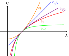
Figure 1: Scale functions $\mathrm{e}_{r},\tilde{\mathrm{e}}_{r}$ associated with the strain tensors $E_{r}$ and $\widetilde{E}_{r}=\frac{1}{2}(E_{r}-E_{-r})$ via eigenvalue $\lambda$.

of material strain tensors, which includes the Biot strain tensor $E_{1\!/\!\!\;2}(U)=U-\@macros@idbb{1}$, the Green-Lagrangian strain tensor $E_{1}(U)=\frac{1}{2}(C-\@macros@idbb{1})=\frac{1}{2}(U^{2}-\@macros@idbb{1})$, where $C=F^{T}F=U^{2}$ is the right Cauchy-Green deformation tensor, the (material) Almansi strain tensor [2] $E_{-1}(U)=\frac{1}{2}(\@macros@idbb{1}-C^{-1})$ and the (material) Hencky strain tensor $E_{0}(U)=\log U$, where $\log\colon\operatorname{Sym^{+}}(n)\to\operatorname{Sym}(n)$ is the principal matrix logarithm [105, p. 20] on the set $\operatorname{Sym^{+}}(n)$ of positive definite symmetric matrices. The Hencky (or logarithmic) strain tensor has often been considered the natural or true strain in nonlinear elasticity [198, 197, 75, 88]. It is also of great importance to so-called hypoelastic models, as is discussed in [210, 76] (cf. Section 4.2.1). A very useful approximation of the material Hencky strain tensor was given by Bažant [17] (cf. [165, 1, 49]):

$$\widetilde{E}_{1\!/\!\!\;2}(U)\;\mathrel{\mathchoice{\vbox{\hbox{$\displaystyle:$}}}{\vbox{\hbox{$\textstyle:$}}}{\vbox{\hbox{$\scriptstyle:$}}}{\vbox{\hbox{$\scriptscriptstyle:$}}}{=}}\;\tfrac{1}{2}\,[E_{1\!/\!\!\;2}(U)+E_{-1\!/\!\!\;2}(U)]\;=\;\tfrac{1}{2}\,(U-U^{-1})\,.$$ (1.4)

Additional motivations of the logarithmic strain tensor were also given by Vallée [205, 206], Rougée [182, p. 302] and Murphy [142]. An extensive overview of the properties of the logarithmic strain tensor and its applications can be found in [209] and [154].

All strain tensors, by the definition employed here, can be seen as equivalent: since the mapping $U\mapsto E(U)$ is injective, for every pair $E,E^{\prime}$ of strain tensors there exists a mapping $\psi\colon\operatorname{Sym}(n)\to\operatorname{Sym}(n)$ such that $E^{\prime}(U)=\psi(E(U))$ for all $U\in\operatorname{Sym^{+}}(n)$. Therefore, every constitutive law of elasticity can – in principle – be expressed in terms of any strain tensor and no strain tensor can be inherently superior to any other strain tensor. Note that this invertibility property also holds if the definition by Hill or Ogden is used: if the strain is given via a scale function $\mathrm{e}$, the strict monotonicity of $\mathrm{e}$ implies that the mapping $U\mapsto E(U)$ is strictly monotone [130], i.e.

$$\langle E(U_{1})-E(U_{2}),U_{1}-U_{2}\rangle>0$$

for all $U_{1},U_{2}\in\operatorname{Sym^{+}}(n)$ with $U_{1}\neq U_{2}$, where $\langle X,Y\rangle=\operatorname{tr}(X^{T}Y)$ denotes the Frobenius inner product on $\operatorname{Sym}(n)$ and $\operatorname{tr}(X)=\sum_{i=1}^{n}X_{i,i}$ is the trace of $X\in\mathbb{R}^{n\times n}$. This monotonicity in turn ensures that the mapping $U\mapsto E(U)$ is injective.

In contrast to strain or strain tensor, we use the term strain measure to refer to a nonnegative real-valued function $\omega\colon\operatorname{GL}^{\!+}(n)\to[0,\infty)$ depending on the deformation gradient which vanishes if and only if $F$ is a pure rotation, i.e. $\omega(F)=0$ if and only if $F\in\operatorname{SO}(n)$.

Note that the terms “strain tensor” and “strain measure” are sometimes used interchangeably in the literature (e.g. [108, 159]). A simple example of a strain measure in the above sense is the mapping $F\mapsto\lVert E(\sqrt{F^{T}F})\rVert$ of $F$ to an orthogonally invariant norm of any strain tensor $E$.

There is a close connection between strain measures and energy functions in isotropic hyperelasticity: an isotropic energy potential [84] is a function $W$ depending on the deformation gradient $F$ such that

$$W(F) \geq 0\,,$$ (normalization)

$$W(QF) =W(F)\,,$$ (frame-indifference)

$$W(FQ) =W(F)$$ (material symmetry: isotropy)

for all $F\in\operatorname{GL}^{\!+}(n),\,Q\in\operatorname{SO}(n)$ and

$$W(F)=0\quad\text{ if and only if }\quad F\in\operatorname{SO}(n)\,.$$ (stress-free reference configuration)

While every such energy function can be taken as a strain measure, many additional conditions for “proper” energy functions are discussed in the literature, such as constitutive inequalities [202, 106, 107, 11, 44, 127], generalized convexity conditions [10, 13] or monotonicity conditions to ensure that “stress increases with strain” [154, Section 2.2]. Apart from that, the main difference between strain measures and energy functions is that the former are purely mathematical expressions used to quantitatively assess the extent of strain in a deformation, whereas the latter postulate some physical behaviour of materials in a condensed form: an elastic energy potential, interpreted as the elastic energy per unit volume in the undeformed configuration, induces a specific stress response function, and therefore completely determines the physical behaviour of the modelled hyperelastic material. The connection between “natural” strain measures and energy functions will be further discussed later on.

In particular, we will be interested in energy potentials which can be expressed in terms of certain strain measures. Note carefully that, in contrast to strain tensors, strain measures cannot simply be used interchangeably: for two different strain measures (as defined above) $\omega_{1},\omega_{2}$, there is generally no function $f\colon\mathbb{R}^{+}\to\mathbb{R}^{+}$ such that $\omega_{2}(F)=f(\omega_{1}(F))$ for all $F\in\operatorname{GL}^{\!+}(n)$. Compared to “full” strain tensors, this can be interpreted as an unavoidable loss of information for strain measures (which are only scalar quantities).

Sometimes a strain measure is employed only for a particular kind of deformation. For example, on the group of simple shear deformations (in a fixed plane) consisting of all $F_{\gamma}\in\operatorname{GL}^{\!+}(3)$ of the form

$$F_{\gamma}=\left(\begin{smallmatrix}1&\gamma&0\\ 0&1&0\\ 0&0&1\end{smallmatrix}\right)\,,\quad\gamma\in\mathbb{R}\,,$$

we could consider the mappings

$$F_{\gamma}\mapsto\frac{1}{2}\,\gamma^{2}\,,\qquad F_{\gamma}\mapsto\frac{1}{\sqrt{3}}\,\lvert\gamma\rvert\qquad\text{ or }\qquad F_{\gamma}\mapsto\frac{2}{\sqrt{3}}\,\ln\left(\frac{\gamma}{2}+\sqrt{1+\frac{\gamma^{2}}{4}}\right);$$

We will come back to these partial strain measures in Section 3.2.

In the following we consider the question of what strain measures are appropriate for the theory of nonlinear isotropic elasticity. Since, by our definition, a strain measure attains zero if and only if $F\in\operatorname{SO}(n)$, a simple geometric approach is to consider a distance function on the group $\operatorname{GL}^{\!+}(n)$ of admissible deformation gradients, i.e. a function $\operatorname{dist}\colon\operatorname{GL}^{\!+}(n)\times\operatorname{GL}^{\!+}(n)\to[0,\infty)$ with $\operatorname{dist}(A,B)=\operatorname{dist}(B,A)$ which satisfies the triangle inequality and vanishes if and only if its arguments are identical. Such a distance function induces a “natural” strain measure on $\operatorname{GL}^{\!+}(n)$ by means of the distance to the special orthogonal group $\operatorname{SO}(n)$:

$$\omega(F)\mathrel{\mathchoice{\vbox{\hbox{$\displaystyle:$}}}{\vbox{\hbox{$\textstyle:$}}}{\vbox{\hbox{$\scriptstyle:$}}}{\vbox{\hbox{$\scriptscriptstyle:$}}}{=}}\operatorname{dist}(F,\operatorname{SO}(n))\mathrel{\mathchoice{\vbox{\hbox{$\displaystyle:$}}}{\vbox{\hbox{$\textstyle:$}}}{\vbox{\hbox{$\scriptstyle:$}}}{\vbox{\hbox{$\scriptscriptstyle:$}}}{=}}\inf_{Q\in\operatorname{SO}(n)}\operatorname{dist}(F,Q)\,.$$ (1.5)

In this way, the search for an appropriate strain measure reduces to the task of finding a natural, intrinsic distance function on $\operatorname{GL}^{\!+}(n)$.

1.2 The search for appropriate strain measures

The remainder of this article is dedicated to this task: after some simple (Euclidean) examples in Section 2, we consider the geodesic distance on $\operatorname{GL}^{\!+}(n)$ in Section 3. Our main result is stated in Theorem 3.3: if the distance on $\operatorname{GL}^{\!+}(n)$ is induced by a left-$\operatorname{GL}(n)$-invariant, right-$\operatorname{O}(n)$-invariant Riemannian metric on $\operatorname{GL}(n)$, then the distance of $F\in\operatorname{GL}^{\!+}(n)$ to $\operatorname{SO}(n)$ is given by

$$\operatorname{dist}_{\mathrm{geod}}^{2}(F,\operatorname{SO}(n))=\operatorname{dist}_{\mathrm{geod}}^{2}(F,R)=\mu\,\lVert\operatorname{dev}_{n}\log U\rVert^{2}+\frac{\kappa}{2}\,[\operatorname{tr}(\log U)]^{2}\,,$$

where $F=R\,U$ with $U=\sqrt{F^{T}F}\in\operatorname{Sym^{+}}(n)$ and $R\in\operatorname{SO}(n)$ is the polar decomposition of $F$. Section 3 also contains some additional remarks and corollaries which further expand upon this Riemannian strain measure.

In Section 4, we discuss a number of different approaches towards motivating the use of logarithmic strain measures and strain tensors, whereas applications of our results and further research topics are indicated in Section 5.

Our main result (Theorem 3.3) has previously been announced in a Comptes Rendus Mécanique article [147] as well as in Proceedings in Applied Mathematics and Mechanics [148].

The idea for this paper was conceived in late 2006. However, a number of technical difficulties had to be overcome (cf. [29, 156, 118, 129, 145]) in order to prove our results. The completion of this article might have taken more time than was originally foreseen, but we adhere to the old German saying: Gut Ding will Weile haben.

2 Euclidean strain measures

2.1 The Euclidean strain measure in linear isotropic elasticity

An approach similar to the definition of strain measures via distance functions on $\operatorname{GL}^{\!+}(n)$, as stated in equation (1.5), can be employed in linearized elasticity theory: let $\varphi(x)=x+u(x)$ with the displacement $u$. Then the infinitesimal strain measure may be obtained by taking the distance of the displacement gradient $\nabla u\in\mathbb{R}^{n\times n}$ to the set of linearized rotations $\operatorname{\mathfrak{so}}(n)=\{A\in\mathbb{R}^{n\times n}:A^{T}=-A\}$, which is the vector space of skew symmetric matrices. An obvious choice for a distance measure on the linear space $\mathbb{R}^{n\times n}\cong\mathbb{R}^{n^{2}}$ of $n\times n$-matrices is the Euclidean distance induced by the canonical Frobenius norm

$$\lVert X\rVert=\sqrt{\operatorname{tr}(X^{T}X)}=\sqrt{\smash{\sum_{i,j=1}^{n}}\vphantom{\sum^{n}}X_{ij}^{2}\,.}\vphantom{\sum_{i,j=1}^{n}}$$

We use the more general weighted norm defined by

$${\lVert X\rVert}_{\mu,\mu_{c},\kappa}^{2}=\mu\,\lVert\operatorname{dev}_{n}\operatorname{sym}X\rVert^{2}+\mu_{c}\,\lVert\mathop{\mathrm{skew}}\nolimits X\rVert^{2}+\frac{\kappa}{2}\,[\operatorname{tr}(X)]^{2}\,,\quad\mu,\mu_{c},\kappa>0\,,$$ (2.1)

which separately weights the deviatoric (or trace free) symmetric part $\operatorname{dev}_{n}\operatorname{sym}X=\operatorname{sym}X-\frac{1}{n}\operatorname{tr}(\operatorname{sym}X)\cdot\@macros@idbb{1}$, the spherical part $\frac{1}{n}\operatorname{tr}(X)\cdot\@macros@idbb{1}$, and the skew symmetric part $\mathop{\mathrm{skew}}\nolimits X=\frac{1}{2}(X-X^{T})$ of $X$; note that ${\lVert X\rVert}_{\mu,\mu_{c},\kappa}=\lVert X\rVert$ for $\mu=\mu_{c}=1,\kappa=\frac{2}{n}$, and that ${\lVert\,.\,\rVert}_{\mu,\mu_{c},\kappa}$ is induced by the inner product

$$\langle X,Y\rangle_{\mu,\mu_{c},\kappa}=\mu\,\langle\operatorname{dev}_{n}\operatorname{sym}X,\operatorname{dev}_{n}\operatorname{sym}Y\rangle+\mu_{c}\,\langle\mathop{\mathrm{skew}}\nolimits X,\mathop{\mathrm{skew}}\nolimits Y\rangle+\tfrac{\kappa}{2}\operatorname{tr}(X)\operatorname{tr}(Y)$$ (2.2)

on $\mathbb{R}^{n\times n}$, where $\langle X,Y\rangle=\operatorname{tr}(X^{T}Y)$ denotes the canonical inner product. In fact, every isotropic inner product on $\mathbb{R}^{n\times n}$, i.e. every inner product $\langle\cdot,\cdot\rangle_{\mathrm{iso}}$ with

$$\langle Q^{T}X\,Q,\;Q^{T}Y\,Q\rangle_{\mathrm{iso}}=\langle X,Y\rangle_{\mathrm{iso}}$$

for all $X,Y\in\mathbb{R}^{n\times n}$ and all $Q\in\operatorname{O}(n)$, is of the form (2.2), cf. [50]. The suggestive choice of variables $\mu$ and $\kappa$, which represent the shear modulus and the bulk modulus, respectively, will prove to be justified later on. The remaining parameter $\mu_{c}$ will be called the spin modulus.

Of course, the element of best approximation in $\operatorname{\mathfrak{so}}(n)$ to $\nabla u$ with respect to the weighted Euclidean distance $\operatorname{dist}_{\mathrm{Euclid,}\mu,\mu_{c},\kappa}(X,Y)={\lVert X-Y\rVert}_{\mu,\mu_{c},\kappa}$ is given by the associated orthogonal projection of $\nabla u$ to $\operatorname{\mathfrak{so}}(n)$, cf. Figure 2. Since $\operatorname{\mathfrak{so}}(n)$ and the space $\operatorname{Sym}(n)$ of symmetric matrices are orthogonal with respect to $\langle\cdot,\cdot\rangle_{\mu,\mu_{c},\kappa}$, this projection is given by the continuum rotation, i.e. the skew symmetric part $\mathop{\mathrm{skew}}\nolimits\nabla u=\frac{1}{2}(\nabla u-(\nabla u)^{T})$ of $\nabla u$, the axial vector of which is $\operatorname{curl}u$. Thus the distance is

$$\operatorname{dist}_{\mathrm{Euclid,}\mu,\mu_{c},\kappa}(\nabla u,\operatorname{\mathfrak{so}}(n)) =\inf_{A\in\operatorname{\mathfrak{so}}(n)}{\lVert\nabla u-A\rVert}_{\mu,\mu_{c},\kappa}$$/

$$={\lVert\nabla u-\mathop{\mathrm{skew}}\nolimits\nabla u\rVert}_{\mu,\mu_{c},\kappa}={\lVert\operatorname{sym}\nabla u\rVert}_{\mu,\mu_{c},\kappa}\,.$$ (2.3)

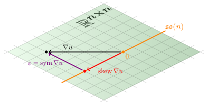
Figure 2: The Euclidean distance $\operatorname{dist}_{\mathrm{Euclid,}\mu,\mu_{c},\kappa}^{2}(\nabla u,\operatorname{\mathfrak{so}}(n))=\mu\,\lVert\operatorname{dev}_{n}\varepsilon\rVert^{2}+\frac{\kappa}{2}\,[\operatorname{tr}(\varepsilon)]^{2}$ of $\nabla u$ to $\operatorname{\mathfrak{so}}(n)$ in $\mathbb{R}^{n\times n}$ in the infinitesimal strain setting. The strain tensor $\varepsilon=\operatorname{sym}\nabla u$ is orthogonal to the infinitesimal continuum rotation $\mathop{\mathrm{skew}}\nolimits\nabla u$.

We therefore find

$$\operatorname{dist}_{\mathrm{Euclid,}\mu,\mu_{c},\kappa}^{2}(\nabla u,\operatorname{\mathfrak{so}}(n)) ={\lVert\operatorname{sym}\nabla u\rVert}_{\mu,\mu_{c},\kappa}^{2}$$

$$=\mu\,\lVert\operatorname{dev}_{n}\operatorname{sym}\nabla u\rVert^{2}+\frac{\kappa}{2}\,[\operatorname{tr}(\operatorname{sym}\nabla u)]^{2}$$

$$=\mu\,\lVert\operatorname{dev}_{n}\varepsilon\rVert^{2}+\frac{\kappa}{2}\,[\operatorname{tr}(\varepsilon)]^{2}=W_{\textrm{lin}}(\nabla u)$$

for the linear strain tensor $\varepsilon=\operatorname{sym}\nabla u$, which is the quadratic isotropic elastic energy, i.e. the canonical model of isotropic linear elasticity with

$$\sigma=D_{\nabla u}W_{\textrm{lin}}(\nabla u)=2\mu\,\operatorname{dev}_{n}\varepsilon+\kappa\operatorname{tr}(\varepsilon)\cdot\@macros@idbb{1}\,.$$ (2.4)

This shows the aforementioned close connection of the energy potential to geometrically motivated measures of strain. Note also that the so computed distance to $\operatorname{\mathfrak{so}}(n)$ is independent of the parameter $\mu_{c}$, the spin modulus, weighting the skew-symmetric part in the quadratic form (2.1). We will encounter the (lack of) influence of the parameter $\mu_{c}$ subsequently again.

Furthermore, this approach motivates the symmetric part $\varepsilon=\operatorname{sym}\nabla u$ of the displacement gradient as the strain tensor in the linear case: instead of postulating that our strain measure should depend only on $\varepsilon$, the above computations deductively characterize $\varepsilon$ as the infinitesimal strain tensor from simple geometric assumptions alone.

2.2 The Euclidean strain measure in nonlinear isotropic elasticity

In order to obtain a strain measure in the geometrically nonlinear case, we must compute the distance

$$\operatorname{dist}(\nabla\varphi,\operatorname{SO}(n))=\operatorname{dist}(F,\operatorname{SO}(n))=\inf_{Q\in\operatorname{SO}(n)}\operatorname{dist}(F,Q)$$

of the deformation gradient $F=\nabla\varphi\in\operatorname{GL}^{\!+}(n)$ to the actual set of pure rotations $\operatorname{SO}(n)\subset\operatorname{GL}^{\!+}(n)$. It is therefore necessary to choose a distance function on $\operatorname{GL}^{\!+}(n)$; an obvious choice is the restriction of the Euclidean distance on $\mathbb{R}^{n\times n}$ to $\operatorname{GL}^{\!+}(n)$. For the canonical Frobenius norm $\lVert\,.\,\rVert$, the Euclidean distance between $F,P\in\operatorname{GL}^{\!+}(n)$ is

$$\operatorname{dist}_{\mathrm{Euclid}}(F,P)=\lVert F-P\rVert=\sqrt{\operatorname{tr}[(F-P)^{T}(F-P)]}\,.$$

Now let $Q\in\operatorname{SO}(n)$. Since $\lVert\,.\,\rVert$ is orthogonally invariant, i.e. $\lVert{\widehat{Q}}X\rVert=\lVert X{\widehat{Q}}\rVert=\lVert X\rVert$ for all $X\in\mathbb{R}^{n\times n}$, ${\widehat{Q}}\in\operatorname{O}(n)$, we find

$$\operatorname{dist}_{\mathrm{Euclid}}(F,Q)=\lVert F-Q\rVert=\lVert Q^{T}(F-Q)\rVert=\lVert Q^{T}F-\@macros@idbb{1}\rVert\,.$$ (2.5)

Thus the computation of the strain measure induced by the Euclidean distance on $\operatorname{GL}^{\!+}(n)$ reduces to the matrix nearness problem [104]

$$\operatorname{dist}_{\mathrm{Euclid}}(F,\operatorname{SO}(n))=\inf_{Q\in\operatorname{SO}(n)}\lVert F-Q\rVert=\min_{Q\in\operatorname{SO}(n)}\lVert Q^{T}F-\@macros@idbb{1}\rVert\,.$$

By a well-known optimality result discovered by Giuseppe Grioli [82] (cf. [150, 83, 131, 31]), also called “Grioli’s Theorem” by Truesdell and Toupin [204, p. 290], this minimum is attained for the orthogonal polar factor $R$.

Theorem 2.1 (Grioli’s Theorem [82, 150, 204]).

Let $F\in\operatorname{GL}^{\!+}(n)$. Then

$$\min_{Q\in\operatorname{SO}(n)}\lVert Q^{T}F-\@macros@idbb{1}\rVert=\lVert R^{T}F-\@macros@idbb{1}\rVert=\lVert\sqrt{F^{T}F}-\@macros@idbb{1}\rVert=\lVert U-\@macros@idbb{1}\rVert\,,$$

where $F=R\,U$ is the polar decomposition of $F$ with $R=\operatorname{polar}(F)\in\operatorname{SO}(n)$ and $U=\sqrt{F^{T}F}\in\operatorname{Sym^{+}}(n)$. The minimum is uniquely attained at the orthogonal polar factor $R$.

Remark 2.2.

The minimization property stated in Theorem 2.1 is equivalent to [132]

$$\max_{Q\in\operatorname{SO}(n)}\operatorname{tr}(Q^{T}F)=\max_{Q\in\operatorname{SO}(n)}\langle Q^{T}F,\@macros@idbb{1}\rangle=\langle R^{T}F,\@macros@idbb{1}\rangle=\langle U,\@macros@idbb{1}\rangle\,.$$

Thus for nonlinear elasticity, the restriction of the Euclidean distance to $\operatorname{GL}^{\!+}(n)$ yields the strain measure

$$\operatorname{dist}_{\mathrm{Euclid}}(F,\operatorname{SO}(n))=\lVert U-\@macros@idbb{1}\rVert\,.$$

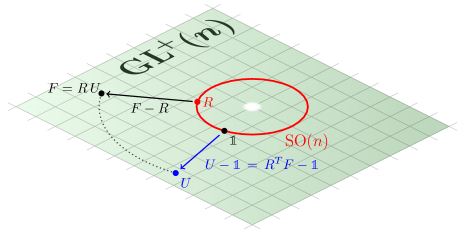
Figure 3: The “flat” interpretation of $\operatorname{GL}^{\!+}(n)\subset\mathbb{R}^{n\times n}$ endowed with the Euclidean distance. Note that $\lVert F-R\rVert=\lVert R\,(U-\@macros@idbb{1})\rVert=\lVert U-\@macros@idbb{1}\rVert$ by orthogonal invariance of the Frobenius norm, where $F=R\,U$ is the polar decomposition of $F$.

In analogy to the linear case, we obtain

$$\operatorname{dist}_{\mathrm{Euclid}}^{2}(F,\operatorname{SO}(n))=\lVert U-\@macros@idbb{1}\rVert^{2}=\lVert E_{1\!/\!\!\;2}\rVert^{2}\,,$$ (2.5)

where $E_{1\!/\!\!\;2}=U-\@macros@idbb{1}$ is the Biot strain tensor. Note the similarity between this expression and the Saint-Venant-Kirchhoff energy [117]

$${\lVert E_{1}\rVert}_{\mu,\mu_{c},\kappa}^{2}=\mu\,\lVert\operatorname{dev}_{3}E_{1}\rVert^{2}+\frac{\kappa}{2}\,[\operatorname{tr}(E_{1})]^{2}\,,$$ (2.6)

where $E_{1}=\frac{1}{2}(C-\@macros@idbb{1})=\frac{1}{2}(U^{2}-\@macros@idbb{1})$ is the Green-Lagrangian strain.

The squared Euclidean distance of $F$ to $\operatorname{SO}(n)$ is often used as a lower bound for more general elastic energy potentials. Friesecke, James and Müller [78], for example, show that if there exists a constant $C>0$ such that

$$W(F)\geq C\cdot\operatorname{dist}_{\mathrm{Euclid}}^{2}(F,\operatorname{SO}(3))$$ (2.7)

for all $F\in\operatorname{GL}^{\!+}(3)$ in a large neighbourhood of $\@macros@idbb{1}$, then the elastic energy $W$ shows some desirable properties which do not otherwise depend on the specific form of $W$. As a starting point for nonlinear theories of bending plates, Friesecke et al. also use the weighted squared norm

$${\lVert\sqrt{F^{T}F}-\@macros@idbb{1}\rVert}_{\mu,\mu_{c},\kappa}^{2}=\mu\,\lVert\operatorname{dev}_{3}(U-\@macros@idbb{1})\rVert^{2}+\frac{\kappa}{2}\,[\operatorname{tr}(U-\@macros@idbb{1})]^{2}=\mu\,\lVert U-\@macros@idbb{1}\rVert^{2}+\frac{\lambda}{2}\,[\operatorname{tr}(U-\@macros@idbb{1})]^{2}\,,$$

where $\lambda$ is the first Lamé parameter, as an energy function satisfying (2.7). The same energy, also called the Biot energy [149], has been recently motivated by applications in digital geometry processing [43].

However, the resulting strain measure $\omega(U)=\operatorname{dist}_{\mathrm{Euclid}}(F,\operatorname{SO}(n))=\lVert U-\@macros@idbb{1}\rVert$ does not truly seem appropriate for finite elasticity theory: for $U\to 0$ we find $\lVert U-\@macros@idbb{1}\rVert\to\lVert\@macros@idbb{1}\rVert=\sqrt{n}<\infty$, thus singular deformations do not necessarily correspond to an infinite measure $\omega$. Furthermore, the above computations are not compatible with the weighted norm introduced in Section 2.1: in general [149, 70, 71],

$$\min_{Q\in\operatorname{SO}(n)}{\lVert F-Q\rVert}_{\mu,\mu_{c},\kappa}^{2}\neq\min_{Q\in\operatorname{SO}(n)}{\lVert Q^{T}F-\@macros@idbb{1}\rVert}_{\mu,\mu_{c},\kappa}^{2}\neq{\lVert\sqrt{F^{T}F}-\@macros@idbb{1}\rVert}_{\mu,\mu_{c},\kappa}^{2}\,,$$ (2.8)

thus the Euclidean distance of $F$ to $\operatorname{SO}(n)$ with respect to ${\lVert\,.\,\rVert}_{\mu,\mu_{c},\kappa}$ does not equal ${\lVert\sqrt{F^{T}F}-\@macros@idbb{1}\rVert}_{\mu,\mu_{c},\kappa}$ in general. In these cases, the element of best approximation is not the orthogonal polar factor $R=\operatorname{polar}(F)$.

In fact, the expression on the left-hand side of (2.8) is not even well defined in terms of linear mappings $F$ and $Q$ [149]: the deformation gradient $F=\nabla\varphi$ at a point $x\in\Omega$ is a two-point tensor and hence, in particular, a linear mapping between the tangent spaces $T_{x}\Omega$ and $T_{\varphi(x)}\varphi(\Omega)$. Since taking the norm

$${\lVert X\rVert}_{\mu,\mu_{c},\kappa}=\mu\,\lVert\operatorname{dev}_{n}\operatorname{sym}X\rVert^{2}+\mu_{c}\,\lVert\mathop{\mathrm{skew}}\nolimits X\rVert^{2}+\frac{\kappa}{2}\,[\operatorname{tr}(X)]^{2}$$

of $X$ requires the decomposition of $X$ into its symmetric and its skew symmetric part, it is only well defined if $X$ is an endomorphism on a single linear space. Therefore ${\lVert F-Q\rVert}_{\mu,\mu_{c},\kappa}$, while being a valid expression for arbitrary matrices $F,Q\in\mathbb{R}^{n\times n}$, is not an admissible term in the setting of finite elasticity.

We also observe that the Euclidean distance is not an intrinsic distance measure on $\operatorname{GL}^{\!+}(n)$: in general, $A-B\notin\operatorname{GL}^{\!+}(n)$ for $A,B\in\operatorname{GL}^{\!+}(n)$, hence the term $\lVert A-B\rVert$ depends on the underlying linear structure of $\mathbb{R}^{n\times n}$. Since it is not a closed subset of $\mathbb{R}^{n\times n}$, $\operatorname{GL}^{\!+}(n)$ is also not complete with respect to $\operatorname{dist}_{\mathrm{Euclid}}$; for example, the sequence $\left(\frac{1}{n}\cdot\@macros@idbb{1}\right)_{n\in\mathbb{N}}$ is a Cauchy sequence which does not converge.

Most importantly, because $\operatorname{GL}^{\!+}(n)$ is not convex, the straight line $\{A+t\,(B-A)\,|\,t\in[0,1]\}$ connecting $A$ and $B$ is not necessarily contained in $\operatorname{GL}^{\!+}(n)$, which shows that the characterization of the Euclidean distance as the length of a shortest connecting curve is also not possible in a way intrinsic to $\operatorname{GL}^{\!+}(n)$, as the intuitive sketches in Figures 4 and 5 indicate.

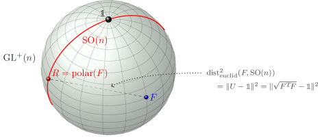
Figure 4: The Euclidean distance as an extrinsic measure on $\operatorname{GL}^{\!+}(n)$.

These issues amply demonstrate that the Euclidean distance can only be regarded as an extrinsic distance measure on the general linear group. We therefore need to expand our view to allow for a more appropriate, truly intrinsic distance measure on $\operatorname{GL}^{\!+}(n)$.

3 The Riemannian strain measure in nonlinear isotropic elasticity

3.1 $\operatorname{GL}^{\!+}(n)$ as a Riemannian manifold

In order to find an intrinsic distance function on $\operatorname{GL}^{\!+}(n)$ that alleviates the drawbacks of the Euclidean distance, we endow $\operatorname{GL}(n)$ with a Riemannian metric. Such a metric $g$ is defined by an inner product

$$g_{A}\colon T_{A}\operatorname{GL}(n)\times T_{A}\operatorname{GL}(n)\to\mathbb{R}$$

on each tangent space $T_{A}\operatorname{GL}(n)$, $A\in\operatorname{GL}(n)$. Then the length of a sufficiently smooth curve $\gamma\colon[0,1]\to\operatorname{GL}(n)$ is given by

$$L(\gamma)=\int_{0}^{1}\sqrt{g_{\gamma(t)}(\dot{\gamma}(t),\dot{\gamma}(t))}\;{\mathrm{d}t}\,,$$

where $\dot{\gamma}(t)=\frac{\mathrm{d}}{\mathrm{d}t}\,\gamma(t)$, and the geodesic distance (cf. Figure 5) between $A,B\in\operatorname{GL}^{\!+}(n)$ is defined as the infimum over the lengths of all (twice continuously differentiable) curves connecting $A$ to $B$:

$$\operatorname{dist}_{\mathrm{geod}}(A,B)=\inf\{L(\gamma)\,|\,\gamma\in C^{2}([0,1];\operatorname{GL}^{\!+}(n)),\;\gamma(0)=A,\;\gamma(1)=B\}\,.$$

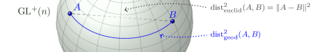
Figure 5: The geodesic (intrinsic) distance compared to the Euclidean (extrinsic) distance.

Our search for an appropriate strain measure is thereby reduced to the task of finding an appropriate Riemannian metric on $\operatorname{GL}(n)$. Although it might appear as an obvious choice, the metric ${\check{g}}$ with

$${\check{g}}_{A}(X,Y)\mathrel{\mathchoice{\vbox{\hbox{$\displaystyle:$}}}{\vbox{\hbox{$\textstyle:$}}}{\vbox{\hbox{$\scriptstyle:$}}}{\vbox{\hbox{$\scriptscriptstyle:$}}}{=}}\langle X,Y\rangle\quad\text{ for all }A\in\operatorname{GL}^{\!+}(n),\;X,Y\in\mathbb{R}^{n\times n}$$ (3.1)

provides no improvement over the already discussed Euclidean distance on $\operatorname{GL}^{\!+}(n)$: since the length of a curve $\gamma$ with respect to ${\check{g}}$ is the classical (Euclidean) length

$$L(\gamma)=\int_{0}^{1}\sqrt{{\check{g}}_{\gamma(t)}(\dot{\gamma}(t),\dot{\gamma}(t))}\,{\mathrm{d}t}=\int_{0}^{1}\lVert\dot{\gamma}(t)\rVert\,{\mathrm{d}t}\,,$$

the shortest connecting curves with respect to ${\check{g}}$ are straight lines of the form $t\mapsto A+t(B-A)$ with $A,B\in\operatorname{GL}^{\!+}(n)$. Locally, the geodesic distance induced by ${\check{g}}$ is therefore equal to the Euclidean distance. However, as discussed in the previous section, not all straight lines connecting arbitrary $A,B\in\operatorname{GL}^{\!+}(n)$ are contained within $\operatorname{GL}^{\!+}(n)$, thus length minimizing curves with respect to ${\check{g}}$ do not necessarily exist (cf. Figure 6). Many of the shortcomings of the Euclidean distance therefore apply to the geodesic distance induced by ${\check{g}}$ as well.

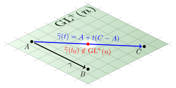
Figure 6: The shortest connecting (geodesic) curves in $\operatorname{GL}^{\!+}(n)$ with respect to the Euclidean metric are straight lines, thus not every pair $A,B\in\operatorname{GL}^{\!+}(n)$ can be connected by curves of minimal length. The length of the straight line $\gamma\colon t\mapsto A+t(B-A)$ connecting $A$ to $B$ is given by $\int_{0}^{1}\sqrt{{\check{g}}_{\gamma(t)}(\dot{\gamma}(t),\dot{\gamma}(t))}\,{\mathrm{d}t}=\lVert B-A\rVert$, whereas the curve $\widehat{\gamma}$ connecting $A$ to $C$ is not contained in $\operatorname{GL}^{\!+}(n)$; its length is therefore not well defined.

In order to find a more viable Riemannian metric $g$ on $\operatorname{GL}(n)$, we consider the mechanical interpretation of the induced geodesic distance $\operatorname{dist}_{\mathrm{geod}}$: while our focus lies on the strain measure induced by $g$, that is the geodesic distance of the deformation gradient $F$ to the special orthogonal group $\operatorname{SO}(n)$, the distance $\operatorname{dist}_{\mathrm{geod}}(F_{1},F_{2})$ between two deformation gradients $F_{1},F_{2}$ can also be motivated directly as a measure of difference between two linear (or homogeneous) deformations $F_{1},F_{2}$ of the same body $\Omega$. More generally, we can define a difference measure between two inhomogeneous deformations $\varphi_{1},\varphi_{2}:\Omega\subset\mathbb{R}^{n}\to\mathbb{R}^{n}$ via

$$\operatorname{dist}(\varphi_{1},\varphi_{2})\mathrel{\mathchoice{\vbox{\hbox{$\displaystyle:$}}}{\vbox{\hbox{$\textstyle:$}}}{\vbox{\hbox{$\scriptstyle:$}}}{\vbox{\hbox{$\scriptscriptstyle:$}}}{=}}\int_{\Omega}\operatorname{dist}_{\mathrm{geod}}(\nabla\varphi_{1}(x),\nabla\varphi_{2}(x))\,{\mathrm{d}x}$$ (3.2)

under suitable regularity conditions for $\varphi_{1},\varphi_{2}$ (e.g. if $\varphi_{1},\varphi_{2}$ are sufficiently smooth with $\det\nabla\varphi_{i}>0$ up to the boundary). This extension of the distance to inhomogeneous deformations is visualized in Figure 7.

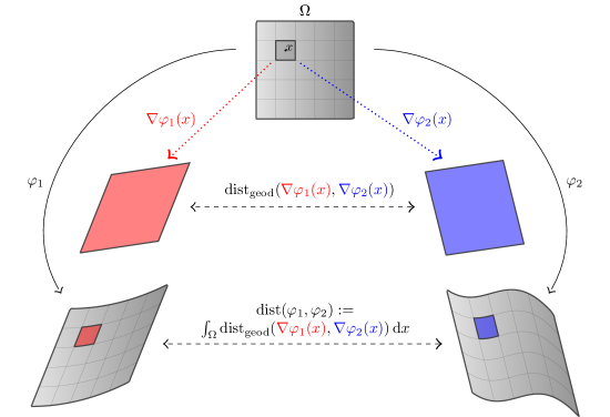
Figure 7: The distance $\operatorname{dist}(\varphi_{1},\varphi_{2})\mathrel{\mathchoice{\vbox{\hbox{$\displaystyle:$}}}{\vbox{\hbox{$\textstyle:$}}}{\vbox{\hbox{$\scriptstyle:$}}}{\vbox{\hbox{$\scriptscriptstyle:$}}}{=}}\int_{\Omega}\operatorname{dist}_{\mathrm{geod}}(\nabla\varphi_{1}(x),\nabla\varphi_{2}(x))\,{\mathrm{d}x}$ measures how much two deformations $\varphi_{1},\varphi_{2}$ of a body $\Omega$ differ from each other via integration over the pointwise geodesic distances between $\nabla\varphi_{1}(x)$ and $\nabla\varphi_{2}(x)$.

In order to find an appropriate Riemannian metric $g$ on $\operatorname{GL}(n)$, we must discuss the required properties of this “difference measure”. First, the requirements of objectivity (left-invariance) and isotropy (right-invariance) suggest that the metric $g$ should be bi-$\operatorname{O}(n)$-invariant, i.e. satisfy

$$\mathrlap{\underbrace{g_{QA}(QX,QY)=g_{A}(X,Y)}_{\text{objectivity}}}\phantom{g_{QA}(QX,QY)=}\overbrace{\phantom{g_{A}(X,Y)}=g_{AQ}(XQ,YQ)}^{\smash{\text{isotropy}}}$$ (3.3)

for all $Q\in\operatorname{O}(n)$, $A\in\operatorname{GL}(n)$ and $X,Y\in T_{A}\operatorname{GL}(n)$, to ensure that $\operatorname{dist}_{\mathrm{geod}}(A,B)=\operatorname{dist}_{\mathrm{geod}}(Q\,A,Q\,B)=\operatorname{dist}_{\mathrm{geod}}(A\,Q,B\,Q)$.

However, these requirements do not sufficiently determine a specific Riemannian metric. For example, (3.3) is satisfied by the metric ${\check{g}}$ defined in (3.1) as well as by the metric ${\check{\check{g}}}$ with ${\check{\check{g}}}_{A}(X,Y)=\langle A^{T}\,X,A^{T}\,Y\rangle$. In order to rule out unsuitable metrics, we need to impose further restrictions on $g$. If we consider the distance measure $\operatorname{dist}(\varphi_{1},\varphi_{2})$ between two deformations $\varphi_{1},\varphi_{2}$ introduced in (3.2), a number of further invariances can be motivated: if we require that the distance is not changed by the superposition of a homogeneous deformation, i.e. that

$$\operatorname{dist}(B\cdot\varphi_{1},B\cdot\varphi_{2})=\operatorname{dist}(\varphi_{1},\varphi_{2})$$

for all constant $B\in\operatorname{GL}(n)$, then $g$ must be left-$\operatorname{GL}(n)$-invariant, i.e.

$$g_{BA}(B\,X,B\,Y)=g_{A}(X,Y)$$ (3.4)

for all $A,B\in\operatorname{GL}(n)$ and $X,Y\in T_{A}\operatorname{GL}(n)$. The physical interpretation of this invariance requirement is readily visualized in Figure 8.

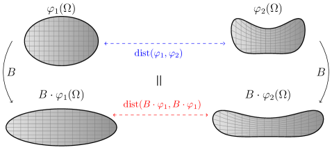
Figure 8: The distance between two deformations should not be changed by the composition with an additional homogeneous transformation $B$: $\operatorname{dist}(\varphi_{1},\varphi_{2})=\operatorname{dist}(B\cdot\varphi_{1},B\cdot\varphi_{2})$.

It can easily be shown [129] that a Riemannian metric $g$ is left-$\operatorname{GL}(n)$-invariant as well as right-$\operatorname{O}(n)$-invariant if and only if $g$ is of the form

$$g_{A}(X,Y)=\langle A^{-1}X,A^{-1}Y\rangle_{\mu,\mu_{c},\kappa}\,,$$ (3.5)

where $\langle\cdot,\cdot\rangle_{\mu,\mu_{c},\kappa}$ is the fixed inner product on the tangent space $\operatorname{\mathfrak{gl}}(n)=T{1}\operatorname{GL}(n)=\mathbb{R}^{n\times n}$ at the identity with

$$\langle X,Y\rangle_{\mu,\mu_{c},\kappa} =\mu\,\langle\operatorname{dev}_{n}\operatorname{sym}X,\operatorname{dev}_{n}\operatorname{sym}Y\rangle+\mu_{c}\langle\mathop{\mathrm{skew}}\nolimits X,\mathop{\mathrm{skew}}\nolimits Y\rangle+\tfrac{\kappa}{2}\operatorname{tr}(X)\operatorname{tr}(Y)$$ (3.6)

for constant positive parameters $\mu,\mu_{c},\kappa>0$, and where $\langle X,Y\rangle=\operatorname{tr}(X^{T}Y)$ denotes the canonical inner product on $\operatorname{\mathfrak{gl}}(n)=\mathbb{R}^{n\times n}$. A Riemannian metric $g$ defined in this way behaves in the same way on all tangent spaces: for every $A\in\operatorname{GL}^{\!+}(n)$, $g$ transforms the tangent space $T_{A}\operatorname{GL}^{\!+}(n)$ at $A$ to the tangent space $T{1}\operatorname{GL}^{\!+}(n)=\operatorname{\mathfrak{gl}}(n)$ at the identity via the left-hand multiplication with $A^{-1}$ and applies the fixed inner product $\langle\cdot,\cdot\rangle_{\mu,\mu_{c},\kappa}$ on $\operatorname{\mathfrak{gl}}(n)$ to the transformed tangents, cf. Figure 9.

In the following, we will always assume that $\operatorname{GL}(n)$ is endowed with a Riemannian metric of the form (3.5) unless indicated otherwise.

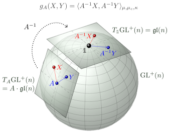
Figure 9: A left-$\operatorname{GL}(n)$-invariant Riemannian metric on $\operatorname{GL}(n)$ transforms the tangent space at $A\in\operatorname{GL}^{\!+}(n)$ to the tangent space $T{1}\operatorname{GL}^{\!+}(n)=\operatorname{\mathfrak{gl}}(n)$ at the identity and applies a fixed inner product on $\operatorname{\mathfrak{gl}}(n)$ to the transformed tangents. Thus no tangent space is treated preferentially.

In order to find the geodesic distance

$$\operatorname{dist}_{\mathrm{geod}}(F,\operatorname{SO}(n))=\inf_{Q\in\operatorname{SO}(n)}\operatorname{dist}_{\mathrm{geod}}(F,Q)$$

of $F\in\operatorname{GL}^{\!+}(n)$ to $\operatorname{SO}(n)$, we need to consider the geodesic curves on $\operatorname{GL}^{\!+}(n)$. It has been shown [129, 134, 87, 5] that every geodesic on $\operatorname{GL}^{\!+}(n)$ with respect to the left-$\operatorname{GL}(n)$-invariant Riemannian metric induced by the inner product (3.6) is of the form

$$\gamma_{F}^{\xi}(t)=F\,\exp(t(\operatorname{sym}\xi-\tfrac{\mu_{c}}{\mu}\mathop{\mathrm{skew}}\nolimits\xi))\,\exp(t(1+\tfrac{\mu_{c}}{\mu})\mathop{\mathrm{skew}}\nolimits\xi)$$ (3.7)

with $F\in\operatorname{GL}^{\!+}(n)$ and some $\xi\in\operatorname{\mathfrak{gl}}(n)$, where $\exp$ denotes the matrix exponential. These curves are characterized by the geodesic equation

$$\dot{\zeta}=\tfrac{\mu+\mu_{c}}{2\mu}(\zeta^{T}\zeta-\zeta\zeta^{T})\,,\qquad\zeta\mathrel{\mathchoice{\vbox{\hbox{$\displaystyle:$}}}{\vbox{\hbox{$\textstyle:$}}}{\vbox{\hbox{$\scriptstyle:$}}}{\vbox{\hbox{$\scriptscriptstyle:$}}}{=}}\gamma^{-1}\dot{\gamma}\,.$$ (3.8)

Since the geodesic curves are defined globally, $\operatorname{GL}^{\!+}(n)$ is geodesically complete with respect to the metric $g$. We can therefore apply the Hopf-Rinow theorem [111, 129] to find that for all $F,P\in\operatorname{GL}^{\!+}(n)$ there exists a length minimizing geodesic $\gamma_{F}^{\xi}$ connecting $F$ and $P$. Without loss of generality, we can assume that $\gamma_{F}^{\xi}$ is defined on the interval $[0,1]$. Then the end points of $\gamma_{F}^{\xi}$ are

$$\gamma_{F}^{\xi}(0)=F\quad\text{ and }\quad P=\gamma_{F}^{\xi}(1)=F\,\exp(\operatorname{sym}\xi-\tfrac{\mu_{c}}{\mu}\mathop{\mathrm{skew}}\nolimits\xi)\,\exp((1+\tfrac{\mu_{c}}{\mu})\mathop{\mathrm{skew}}\nolimits\xi)\,,$$

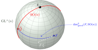
Figure 11: The geodesic (intrinsic) distance to $\operatorname{SO}(n)$; neither the element ${\widehat{Q}}$ of best approximation nor the initial tangent $F\,\xi\in T_{F}\operatorname{GL}^{\!+}(n)$ of the connecting geodesic is known beforehand.

and the length of the geodesic $\gamma_{F}^{\xi}$ starting in $F$ with initial tangent $F\,\xi\in T_{F}\operatorname{GL}^{\!+}(n)$ (cf. (3.7) and Figure 11) is given by [129]

$$L(\gamma_{F}^{\xi})={\lVert\xi\rVert}_{\mu,\mu_{c},\kappa}\,.$$

The geodesic distance between $F$ and $P$ can therefore be characterized as

$$\operatorname{dist}_{\mathrm{geod}}(F,P)=\min\{{\lVert\xi\rVert}_{\mu,\mu_{c},\kappa}\,|\,\;\xi\in\operatorname{\mathfrak{gl}}(n):\,\gamma_{F}^{\xi}(1)=P\}\,,$$

that is the minimum of ${\lVert\xi\rVert}_{\mu,\mu_{c},\kappa}$ over all $\xi\in\operatorname{\mathfrak{gl}}(n)$ which connect $F$ and $P$, i.e. satisfy

$$\exp(\operatorname{sym}\xi-\tfrac{\mu_{c}}{\mu}\mathop{\mathrm{skew}}\nolimits\xi)\,\exp((1+\tfrac{\mu_{c}}{\mu})\mathop{\mathrm{skew}}\nolimits\xi)=F^{-1}P\,.$$ (3.9)

Although some numerical computations have been employed [215] to approximate the geodesic distance in the special case of the canonical left-$\operatorname{GL}(n)$-invariant metric, i.e. for $\mu=\mu_{c}=1$, $\kappa=\frac{2}{n}$, there is no known closed form solution to the highly nonlinear system (3.9) in terms of $\xi$ for given $F,P\in\operatorname{GL}^{\!+}(n)$ and thus no known method of directly computing $\operatorname{dist}_{\mathrm{geod}}(F,P)$ in the general case exists. However, this parametrization of the geodesic curves will still allow us to obtain a lower bound on the distance of $F$ to $\operatorname{SO}(n)$.

3.2 The geodesic distance to $\operatorname{SO}(n)$

Having defined the geodesic distance on $\operatorname{GL}^{\!+}(n)$, we can now consider the geodesic strain measure, which is the geodesic distance of the deformation gradient $F$ to $\operatorname{SO}(n)$:

$$\operatorname{dist}_{\mathrm{geod}}(F,\operatorname{SO}(n))=\inf_{Q\in\operatorname{SO}(n)}\operatorname{dist}_{\mathrm{geod}}(F,Q)\,.$$ (3.10)

Without explicit computation of this distance, the left-$\operatorname{GL}(n)$-invariance and the right-$\operatorname{O}(n)$-invariance of the metric $g$ immediately allow us to show the inverse deformation symmetry of the geodesic strain measure:

$$\operatorname{dist}_{\mathrm{geod}}(F,\operatorname{SO}(n)) =\inf_{Q\in\operatorname{SO}(n)}\operatorname{dist}_{\mathrm{geod}}(F,Q) =\inf_{Q\in\operatorname{SO}(n)}\operatorname{dist}_{\mathrm{geod}}(F^{-1}F,F^{-1}Q)$$

$$=\inf_{Q\in\operatorname{SO}(n)}\operatorname{dist}_{\mathrm{geod}}(\@macros@idbb{1},F^{-1}Q)\; =\inf_{Q\in\operatorname{SO}(n)}\operatorname{dist}_{\mathrm{geod}}(Q^{T}Q,F^{-1}Q)$$

$$=\inf_{Q\in\operatorname{SO}(n)}\operatorname{dist}_{\mathrm{geod}}(Q^{T},F^{-1}) =\;\operatorname{dist}_{\mathrm{geod}}(F^{-1},\operatorname{SO}(n))\,.$$ (3.11)

This symmetry property demonstrates at once that the Eulerian (spatial) and the Lagrangian (referential) points of view are equivalent with respect to the geodesic strain measure: in the Eulerian setting, the inverse $F^{-1}$ of the deformation gradient appears more naturally, whereas $F$ is used in the Lagrangian frame (cf. Figure 10). Equality (3.11) shows that both points of view can equivalently be taken if the geodesic strain measure is used. As we will see later on (Remark 3.5), the equality $\operatorname{dist}_{\mathrm{geod}}(B,\operatorname{SO}(n))=\operatorname{dist}_{\mathrm{geod}}(C,\operatorname{SO}(n))$ also holds for the right Cauchy-Green deformation tensor $C=F^{T}F=U^{2}$ and the Finger tensor $B=FF^{T}=V^{2}$, further indicating the independence of the geodesic strain measure from the chosen frame of reference. This property is, however, not unique to geodesic (or logarithmic) strain measures; for example, the Frobenius norm

$$\lVert\widetilde{E}_{1\!/\!\!\;2}(U)\rVert=\tfrac{1}{2}\lVert U-U^{-1}\rVert=\tfrac{1}{2}\lVert V-V^{-1}\rVert$$

of the Bažant approximation $\widetilde{E}_{1\!/\!\!\;2}=\frac{1}{2}\,(U-U^{-1})$, cf. (1.4) and [17], which can be considered a “quasilogarithmic” strain measure, fulfils the inverse deformation symmetry as well. However, it is not satisfied for the Euclidean distance to $\operatorname{SO}(n)$: in general,

$$\lVert U-\@macros@idbb{1}\rVert=\operatorname{dist}_{\mathrm{Euclid}}(F,\operatorname{SO}(n))\neq\operatorname{dist}_{\mathrm{Euclid}}(F^{-1},\operatorname{SO}(n))=\lVert V^{-1}-\@macros@idbb{1}\rVert\,.$$ (3.12)

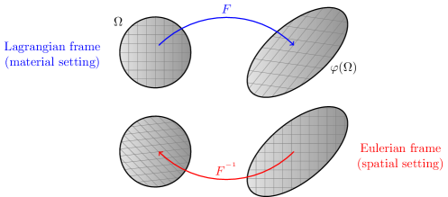
Figure 10: The Lagrangian and the Eulerian point of view are equivalently represented by the geodesic strain measure: $\operatorname{dist}_{\mathrm{geod}}(F,\operatorname{SO}(n))=\operatorname{dist}_{\mathrm{geod}}(F^{-1},\operatorname{SO}(n))$.

Now, let $F=R\,U$ denote the polar decomposition of $F$ with $U\in\operatorname{Sym^{+}}(n)$ and $R\in\operatorname{SO}(n)$. In order to establish a simple upper bound on the geodesic distance $\operatorname{dist}_{\mathrm{geod}}(F,\operatorname{SO}(n))$, we construct a particular curve $\gamma_{R}$ connecting $F$ to its orthogonal factor $R\in\operatorname{SO}(n)$ and compute its length $L(\gamma_{R})$. For

$$\gamma_{R}(t)\mathrel{\mathchoice{\vbox{\hbox{$\displaystyle:$}}}{\vbox{\hbox{$\textstyle:$}}}{\vbox{\hbox{$\scriptstyle:$}}}{\vbox{\hbox{$\scriptscriptstyle:$}}}{=}}R\,\exp((1-t)\,\log U)\,,$$

where $\log U\in\operatorname{Sym}(n)$ is the principal matrix logarithm of $U$, we find

$$\gamma_{R}(0)=R\,\exp(\log U)=R\,U=F\qquad\text{ and }\qquad\gamma_{R}(1)=R\,\exp(0)=R\in\operatorname{SO}(n)\,.$$

It is easy to confirm that $\gamma_{R}$ is in fact a geodesic as given in (3.7) with $\xi=\log U\in\operatorname{Sym}(n)$. Since

$$\gamma_{R}^{-1}(t)\dot{\gamma}_{R}(t)=(R\,\exp((1-t)\,\log U))^{-1}\;R\,\exp((1-t)\,\log U)\cdot(-\log U)=-\log U\,,$$

the length of $\gamma_{R}$ is given by

$$L(\gamma_{R}) =\int_{0}^{1}\sqrt{g_{\gamma_{R}(t)}(\dot{\gamma}_{R}(t),\dot{\gamma}_{R}(t))}\;{\mathrm{d}t}$$ (3.13)

$$=\int_{0}^{1}\sqrt{\langle\gamma_{R}(t)^{-1}\dot{\gamma}_{R}(t),\gamma_{R}(t)^{-1}\dot{\gamma}_{R}(t)\rangle_{\mu,\mu_{c},\kappa}}\;{\mathrm{d}t}$$

$$=\int_{0}^{1}\sqrt{\langle-\log U,-\log U\rangle_{\mu,\mu_{c},\kappa}}\;{\mathrm{d}t}=\int_{0}^{1}{\lVert\log U\rVert}_{\mu,\mu_{c},\kappa}\,{\mathrm{d}t}={\lVert\log U\rVert}_{\mu,\mu_{c},\kappa}\,.$$

We can thereby establish the upper bound

$$\operatorname{dist}_{\mathrm{geod}}^{2}(F,\operatorname{SO}(n)) =\inf_{Q\in\operatorname{SO}(n)}\operatorname{dist}_{\mathrm{geod}}^{2}(F,Q)\leq\operatorname{dist}_{\mathrm{geod}}^{2}(F,R)$$ (3.14)

$$\leq L^{2}(\gamma_{R})={\lVert\log U\rVert}_{\mu,\mu_{c},\kappa}^{2}=\mu\,\lVert\operatorname{dev}_{n}\log U\rVert^{2}+\frac{\kappa}{2}\,[\operatorname{tr}(\log U)]^{2}$$ (3.15)

for the geodesic distance of $F$ to $\operatorname{SO}(n)$.

Our task in the remainder of this section is to show that the right hand side of inequality (3.15) is also a lower bound for the (squared) geodesic strain measure, i.e. that, altogether,

$$\operatorname{dist}_{\mathrm{geod}}^{2}(F,\operatorname{SO}(n))=\mu\,\lVert\operatorname{dev}_{n}\log U\rVert^{2}+\frac{\kappa}{2}\,[\operatorname{tr}(\log U)]^{2}\,.$$

However, while the orthogonal polar factor $R$ is the element of best approximation in the Euclidean case (for $\mu=\mu_{c}=1$, $\kappa=\frac{2}{n}$) due to Grioli’s Theorem, it is not clear whether $R$ is indeed the element in $\operatorname{SO}(n)$ with the shortest geodesic distance to $F$ (and thus whether equality holds in (3.14)). Furthermore, it is not even immediately obvious that the geodesic distance between $F$ and $R$ is actually given by the right hand side of (3.15), since a shorter connecting geodesic might exist (and hence inequality might hold in (3.15)).

Nonetheless, the following fundamental logarithmic minimization property of the orthogonal polar factor, combined with the computations in Section 3.1, allows us to show that (3.15) is indeed also a lower bound for $\operatorname{dist}_{\mathrm{geod}}(F,\operatorname{SO}(n))$.

Proposition 3.1.

Let $F=R\,\sqrt{F^{T}F}$ be the polar decomposition of $F\in\operatorname{GL}^{\!+}(n)$ with $R\in\operatorname{SO}(n)$ and let $\lVert\,.\,\rVert$ denote the Frobenius norm on $\mathbb{R}^{n\times n}$. Then

$$\inf_{Q\in\operatorname{SO}(n)}\lVert\operatorname{sym}\operatorname{Log}(Q^{T}F)\rVert=\lVert\operatorname{sym}\log(R^{T}F)\rVert=\lVert\log\sqrt{F^{T}F}\rVert\,,$$

where

$$\inf_{Q\in\operatorname{SO}(n)}\lVert\operatorname{sym}\operatorname{Log}(Q^{T}F)\rVert\mathrel{\mathchoice{\vbox{\hbox{$\displaystyle:$}}}{\vbox{\hbox{$\textstyle:$}}}{\vbox{\hbox{$\scriptstyle:$}}}{\vbox{\hbox{$\scriptscriptstyle:$}}}{=}}\inf_{Q\in\operatorname{SO}(n)}\inf\{\lVert\operatorname{sym}X\rVert\;\,|\,\;X\in\mathbb{R}^{n\times n}\,,\;\exp(X)=Q^{T}F\}$$

is defined as the infimum of $\lVert\operatorname{sym}\,.\,\rVert$ over “all real matrix logarithms” of $Q^{T}F$.

Proposition 3.1, which can be seen as the natural logarithmic analogue of Grioli’s Theorem (cf. Section 2.2), was first shown for dimensions $n=2,3$ by Neff et al. [156] using the so-called sum-of-squared-logarithms inequality [29, 170, 48, 30]. A generalization to all unitarily invariant norms and complex logarithms for arbitrary dimension was given by Lankeit, Neff and Nakatsukasa [118]. We also require the following corollary involving the weighted Frobenius norm, which is not orthogonally invariant.

Corollary 3.2.

Let

$${\lVert X\rVert}_{\mu,\mu_{c},\kappa}^{2}=\mu\,\lVert\operatorname{dev}_{n}\operatorname{sym}X\rVert^{2}+\mu_{c}\,\lVert\mathop{\mathrm{skew}}\nolimits X\rVert^{2}+\frac{\kappa}{2}\,[\operatorname{tr}(X)]^{2}\,,\qquad\mu,\mu_{c},\kappa>0\,,$$

for all $X\in\mathbb{R}^{n\times n}$, where $\lVert\,.\,\rVert$ is the Frobenius matrix norm. Then

$$\inf_{Q\in\operatorname{SO}(n)}{\lVert\operatorname{sym}\operatorname{Log}(Q^{T}F)\rVert}_{\mu,\mu_{c},\kappa}={\lVert\log\sqrt{F^{T}F}\rVert}_{\mu,\mu_{c},\kappa}\,.$$

Proof.

We first note that the equality $\det\exp(X)=e^{\operatorname{tr}(X)}$ holds for all $X\in\mathbb{R}^{n\times n}$. Since $\det Q=1$ for all $Q\in\operatorname{SO}(n)$, this implies that for all $X\in\mathbb{R}^{n\times n}$ with $\exp(X)=Q^{T}F$,

$$\operatorname{tr}(\operatorname{sym}X)=\operatorname{tr}(X)=\ln(\det(\exp(X)))=\ln(\det(Q^{T}F))=\ln(\det F)\,.$$

Therefore

$${\lVert\operatorname{sym}X\rVert}_{\mu,\mu_{c},\kappa}^{2} =\mu\,\lVert\operatorname{dev}_{n}\operatorname{sym}X\rVert^{2}+\frac{\kappa}{2}\,[\operatorname{tr}(\operatorname{sym}X)]^{2}$$

$$=\mu\,\lVert\operatorname{sym}X\rVert^{2}+\frac{n\,\kappa-2\mu}{2n}\,[\operatorname{tr}(\operatorname{sym}X)]^{2}=\mu\,\lVert\operatorname{sym}X\rVert^{2}+\frac{n\,\kappa-2\mu}{2n}\,(\ln(\det F))^{2}$$

and finally

$$\inf_{Q\in\operatorname{SO}(n)}{\lVert\operatorname{sym}\operatorname{Log}(Q^{T}F)\rVert}_{\mu,\mu_{c},\kappa}^{2}$$ (3.16)

$$=\inf_{Q\in\operatorname{SO}(n)}\inf\{{\lVert\operatorname{sym}X\rVert}_{\mu,\mu_{c},\kappa}^{2}\,|\,X\in\mathbb{R}^{n\times n}\,,\;\exp(X)=Q^{T}F\}$$

$$=\inf_{Q\in\operatorname{SO}(n)}\inf\{\mu\,\lVert\operatorname{sym}X\rVert^{2}+\frac{n\,\kappa-2\mu}{2n}\,(\ln(\det F))^{2}\,|\,X\in\mathbb{R}^{n\times n}\,,\;\exp(X)=Q^{T}F\}$$

$$=\mu\inf_{Q\in\operatorname{SO}(n)}\inf\{\lVert\operatorname{sym}X\rVert^{2}\,|\,X\in\mathbb{R}^{n\times n}\,,\;\exp(X)=Q^{T}F\}+\frac{n\,\kappa-2\mu}{2n}\,(\ln(\det F))^{2}$$

$$=\mu\lVert\log\sqrt{F^{T}F}\rVert^{2}+\frac{n\,\kappa-2\mu}{2n}\,(\ln(\det F))^{2}$$

$$=\mu\lVert\log\sqrt{F^{T}F}\rVert^{2}+\frac{n\,\kappa-2\mu}{2n}\,[\operatorname{tr}(\log\sqrt{F^{T}F})]^{2}$$

$$=\mu\,\lVert\operatorname{dev}_{n}\log\sqrt{F^{T}F}\rVert^{2}+\frac{\kappa}{2}\,[\operatorname{tr}(\log\sqrt{F^{T}F})]^{2}={\lVert\log\sqrt{F^{T}F}\rVert}_{\mu,\mu_{c},\kappa}^{2}\,.\qed$$

Note that Corollary 3.2 also implies the slightly weaker statement

$$\inf_{Q\in\operatorname{SO}(n)}{\lVert\operatorname{Log}(Q^{T}F)\rVert}_{\mu,\mu_{c},\kappa}={\lVert\log\sqrt{F^{T}F}\rVert}_{\mu,\mu_{c},\kappa}$$

by using the simple estimate ${\lVert X\rVert}_{\mu,\mu_{c},\kappa}^{2}\geq{\lVert\operatorname{sym}X\rVert}_{\mu,\mu_{c},\kappa}^{2}$.
We are now ready to prove our main result.

Theorem 3.3.

Let $g$ be the left-$\operatorname{GL}(n)$-invariant, right-$\operatorname{O}(n)$-invariant Riemannian metric on $\operatorname{GL}(n)$ defined by

$$g_{A}(X,Y)=\langle A^{-1}X,A^{-1}Y\rangle_{\mu,\mu_{c},\kappa}\,,\qquad\mu,\mu_{c},\kappa>0\,,$$

for $A\in\operatorname{GL}(n)$ and $X,Y\in\mathbb{R}^{n\times n}$, where

$$\langle X,Y\rangle_{\mu,\mu_{c},\kappa}=\mu\,\langle\operatorname{dev}_{n}\operatorname{sym}X,\operatorname{dev}_{n}\operatorname{sym}Y\rangle+\mu_{c}\langle\mathop{\mathrm{skew}}\nolimits X,\mathop{\mathrm{skew}}\nolimits Y\rangle+\tfrac{\kappa}{2}\operatorname{tr}(X)\operatorname{tr}(Y)\,.$$ (3.17)

Then for all $F\in\operatorname{GL}^{\!+}(n)$, the geodesic distance of $F$ to the special orthogonal group $\operatorname{SO}(n)$ induced by $g$ is given by

$$\operatorname{dist}_{\mathrm{geod}}^{2}(F,\operatorname{SO}(n))=\mu\,\lVert\operatorname{dev}_{n}\log U\rVert^{2}+\frac{\kappa}{2}\,[\operatorname{tr}(\log U)]^{2}\,,$$ (3.18)

where $\log$ is the principal matrix logarithm, $\operatorname{tr}(X)=\sum_{i=1}^{n}X_{i,i}$ denotes the trace and $\operatorname{dev}_{n}X=X-\frac{1}{n}\operatorname{tr}(X)\cdot\@macros@idbb{1}$ is the $n$-dimensional deviatoric part of $X\in\mathbb{R}^{n\times n}$. The orthogonal factor $R\in\operatorname{SO}(n)$ of the polar decomposition $F=R\,U$ is the unique element of best approximation in $\operatorname{SO}(n)$, i.e.

$$\operatorname{dist}_{\mathrm{geod}}(F,\operatorname{SO}(n))=\operatorname{dist}_{\mathrm{geod}}(F,R)=\operatorname{dist}_{\mathrm{geod}}(R^{T}F,\@macros@idbb{1})=\operatorname{dist}_{\mathrm{geod}}(U,\@macros@idbb{1})\,.$$

In particular, the geodesic distance does not depend on the spin modulus $\mu_{c}$.

Remark 3.4 (Uniqueness of the metric).

We remark once more that the Riemannian metric considered in Theorem 3.3 is not chosen arbitrarily: every left-$\operatorname{GL}(n)$-invariant, right-$\operatorname{O}(n)$-invariant Riemannian metric on $\operatorname{GL}(n)$ is of the form given in (3.17) for some choice of parameters $\mu,\mu_{c},\kappa>0$ [129]. $\square$

Remark 3.5.

Since the weighted Frobenius norm on the right hand side of equation (3.18) only depends on the eigenvalues of $U=\sqrt{F^{T}F}$, the result can also be expressed in terms of the left Biot-stretch tensor $V=\sqrt{FF^{T}}$, which has the same eigenvalues as $U$:

$$\operatorname{dist}_{\mathrm{geod}}^{2}(F,\operatorname{SO}(n))=\mu\,\lVert\operatorname{dev}_{n}\log V\rVert^{2}+\frac{\kappa}{2}\,[\operatorname{tr}(\log V)]^{2}\,.$$ (3.19)

Applying the above formula to the case $F=P$ with $P\in\operatorname{Sym^{+}}(n)$, we find $\sqrt{P^{T}P}=\sqrt{PP^{T}}=P$ and therefore

$$\operatorname{dist}^{2}(P,\operatorname{SO}(n))=\operatorname{dist}^{2}(P,\,\@macros@idbb{1})=\mu\,\lVert\operatorname{dev}_{n}\log P\rVert^{2}+\frac{\kappa}{2}\,[\operatorname{tr}(\log P)]^{2}\,,$$ (3.20)

since $\@macros@idbb{1}$ is the orthogonal polar factor of $P$. For the tensors $U$ and $V$, the right Cauchy-Green deformation tensor $C=F^{T}F=U^{2}$ and the Finger tensor $B=FF^{T}=V^{2}$, we thereby obtain the equalities

$$\operatorname{dist}_{\mathrm{geod}}(B,\operatorname{SO}(n)) =\operatorname{dist}_{\mathrm{geod}}(B,\@macros@idbb{1}) =\operatorname{dist}_{\mathrm{geod}}(B^{-1},\@macros@idbb{1})$$ (3.21)

$$=\operatorname{dist}_{\mathrm{geod}}(C,\@macros@idbb{1}) =\operatorname{dist}_{\mathrm{geod}}(C^{-1},\@macros@idbb{1}) =\operatorname{dist}_{\mathrm{geod}}(C,\operatorname{SO}(n))$$

and $$\operatorname{dist}_{\mathrm{geod}}(V,\operatorname{SO}(n)) =\operatorname{dist}_{\mathrm{geod}}(V,\@macros@idbb{1}) =\operatorname{dist}_{\mathrm{geod}}(V^{-1},\@macros@idbb{1})$$ (3.22)

$$=\operatorname{dist}_{\mathrm{geod}}(U,\@macros@idbb{1}) =\operatorname{dist}_{\mathrm{geod}}(U^{-1},\@macros@idbb{1}) =\operatorname{dist}_{\mathrm{geod}}(U,\operatorname{SO}(n))\,.$$

Note carefully that, although (3.20) for $P\in\operatorname{Sym^{+}}(n)$ immediately follows from Theorem 3.3, it is not trivial to compute the distance $\operatorname{dist}_{\mathrm{geod}}(P,\,\@macros@idbb{1})$ directly: while the curve given by $\exp(t\,\log P)$ for $t\in[0,1]$ is in fact a geodesic [87] connecting $\@macros@idbb{1}$ to $P$ with squared length $\mu\,\lVert\operatorname{dev}_{n}\log P\rVert^{2}+\frac{\kappa}{2}\,[\operatorname{tr}(\log P)]^{2}$, it is not obvious whether or not a shorter connecting geodesic might exist. Our result ensures that this is in fact not the case. $\square$

Proof of Theorem 3.3.

Let $F\in\operatorname{GL}^{\!+}(n)$ and ${\widehat{Q}}\in\operatorname{SO}(n)$. Then according to our previous considerations (cf. Section 3.1) there exists $\xi\in\operatorname{\mathfrak{gl}}(n)$ with

$$\exp(\operatorname{sym}\xi-\tfrac{\mu_{c}}{\mu}\mathop{\mathrm{skew}}\nolimits\xi)\,\exp((1+\tfrac{\mu_{c}}{\mu})\mathop{\mathrm{skew}}\nolimits\xi)=F^{-1}{\widehat{Q}}$$ (3.23)

and

$${\lVert\xi\rVert}_{\mu,\mu_{c},\kappa}=\operatorname{dist}_{\mathrm{geod}}(F,{\widehat{Q}})\,.$$ (3.24)

In order to find a lower estimate on ${\lVert\xi\rVert}_{\mu,\mu_{c},\kappa}$ (and thus on $\operatorname{dist}_{\mathrm{geod}}(F,{\widehat{Q}})$), we compute

$$\exp(\operatorname{sym}\xi-\tfrac{\mu_{c}}{\mu}\mathop{\mathrm{skew}}\nolimits\xi)\,\exp((1+\tfrac{\mu_{c}}{\mu})\mathop{\mathrm{skew}}\nolimits\xi) =F^{-1}{\widehat{Q}}$$

$$\Longrightarrow\quad \exp((1+\tfrac{\mu_{c}}{\mu})\mathop{\mathrm{skew}}\nolimits\xi)^{-1}\,\exp(\operatorname{sym}\xi-\tfrac{\mu_{c}}{\mu}\mathop{\mathrm{skew}}\nolimits\xi)^{-1} ={\widehat{Q}}^{T}F$$

$$\Longrightarrow\quad \exp(-\operatorname{sym}\xi+\tfrac{\mu_{c}}{\mu}\mathop{\mathrm{skew}}\nolimits\xi) =\exp(\,\underbrace{(1+\tfrac{\mu_{c}}{\mu})\mathop{\mathrm{skew}}\nolimits\xi}_{\in\operatorname{\mathfrak{so}}(n)}\,)\,{\widehat{Q}}^{T}F\,.$$

Since $\exp(W)\in\operatorname{SO}(n)$ for all skew symmetric $W\in\operatorname{\mathfrak{so}}(n)$, we find

$$\exp(\underbrace{-\operatorname{sym}\xi+\tfrac{\mu_{c}}{\mu}\mathop{\mathrm{skew}}\nolimits\xi}_{\mathrel{{=}\mathchoice{\vbox{\hbox{$\displaystyle:$}}}{\vbox{\hbox{$\textstyle:$}}}{\vbox{\hbox{$\scriptstyle:$}}}{\vbox{\hbox{$\scriptscriptstyle:$}}}}Y})=Q_{\xi}^{T}F$$ (3.25)

with $Q_{\xi}={\widehat{Q}}\,\exp(-(1+\tfrac{\mu_{c}}{\mu})\mathop{\mathrm{skew}}\nolimits\xi\,)\in\operatorname{SO}(n)$; note that $\operatorname{sym}Y=-\operatorname{sym}\xi$. According to (3.25), $Y=-\operatorname{sym}\xi+\tfrac{\mu_{c}}{\mu}\mathop{\mathrm{skew}}\nolimits\xi$ is “a logarithm” of $Q_{\xi}^{T}F$. The weighted Frobenius norm of the symmetric part of  $Y=-\operatorname{sym}\xi+\tfrac{\mu_{c}}{\mu}\mathop{\mathrm{skew}}\nolimits\xi$ is therefore bounded below by the infimum of ${\lVert\operatorname{sym}X\rVert}_{\mu,\mu_{c},\kappa}$ over “all logarithms” $X$ of $Q_{\xi}^{T}F$:

$${\lVert\operatorname{sym}\xi\rVert}_{\mu,\mu_{c},\kappa} ={\lVert\operatorname{sym}Y\rVert}_{\mu,\mu_{c},\kappa}$$

$$\overset{\mathclap{\eqref{eq:termIsLogOfQTxiF}}}{\geq}\hphantom{\inf_{Q\in\operatorname{SO}(n)}}\inf\{{\lVert\operatorname{sym}X\rVert}_{\mu,\mu_{c},\kappa}\,|\,X\in\mathbb{R}^{n\times n}\,,\;\exp(X)=Q_{\xi}^{T}F\}$$

$$\geq\inf_{Q\in\operatorname{SO}(n)}\inf\{{\lVert\operatorname{sym}X\rVert}_{\mu,\mu_{c},\kappa}\,|\,X\in\mathbb{R}^{n\times n}\,,\;\exp(X)=Q^{T}F\}$$

$$=\inf_{Q\in\operatorname{SO}(n)}{\lVert\operatorname{sym}\operatorname{Log}(Q^{T}F)\rVert}_{\mu,\mu_{c},\kappa}\,.$$ (3.26)

We can now apply Corollary 3.2 to find

$$\operatorname{dist}_{\mathrm{geod}}^{2}(F,{\widehat{Q}})={\lVert\xi\rVert}_{\mu,\mu_{c},\kappa}^{2} =\mu\,\lVert\operatorname{dev}_{n}\operatorname{sym}\xi\rVert^{2}+\mu_{c}\,\lVert\mathop{\mathrm{skew}}\nolimits\xi\rVert^{2}+\frac{\kappa}{2}\,[\operatorname{tr}(\operatorname{sym}\xi)]^{2}$$

$$\geq\mu\,\lVert\operatorname{dev}_{n}\operatorname{sym}\xi\rVert^{2}+\frac{\kappa}{2}\,[\operatorname{tr}(\operatorname{sym}\xi)]^{2}$$ (3.27)

$$={\lVert\operatorname{sym}\xi\rVert}_{\mu,\mu_{c},\kappa}^{2}$$

$$\overset{\mathclap{\eqref{eq:inequalityForSymXi}}}{\geq}\inf_{Q\in\operatorname{SO}(n)}{\lVert\operatorname{sym}\operatorname{Log}(Q^{T}F)\rVert}_{\mu,\mu_{c},\kappa}^{2}$$

$$\overset{\mathclap{\text{Corollary \ref{cor:infLogWeighted}}}}{=}\qquad\mu\,{\lVert\log\sqrt{F^{T}F}\rVert}_{\mu,\mu_{c},\kappa}^{2}=\mu\,\lVert\operatorname{dev}_{n}\log U\rVert^{2}+\frac{\kappa}{2}\,[\operatorname{tr}(\log U)]^{2}$$

for $U=\sqrt{F^{T}F}$. Since this inequality is independent of ${\widehat{Q}}$ and holds for all ${\widehat{Q}}\in\operatorname{SO}(n)$, we obtain the desired lower bound

$$\operatorname{dist}_{\mathrm{geod}}^{2}(F,\operatorname{SO}(n))=\inf_{{\widehat{Q}}\in\operatorname{SO}(n)}\operatorname{dist}_{\mathrm{geod}}^{2}(F,{\widehat{Q}})\geq\mu\,\lVert\operatorname{dev}_{n}\log U\rVert^{2}+\frac{\kappa}{2}\,[\operatorname{tr}(\log U)]^{2}$$

on the geodesic distance of $F$ to $\operatorname{SO}(n)$. Together with the upper bound

$$\operatorname{dist}_{\mathrm{geod}}^{2}(F,\operatorname{SO}(n))\leq\operatorname{dist}_{\mathrm{geod}}^{2}(F,R)\leq\mu\,\lVert\operatorname{dev}_{n}\log U\rVert^{2}+\frac{\kappa}{2}\,[\operatorname{tr}(\log U)]^{2}$$

already established in (3.15), we finally find

$$\operatorname{dist}_{\mathrm{geod}}^{2}(F,\operatorname{SO}(n))=\operatorname{dist}_{\mathrm{geod}}^{2}(F,R)=\mu\,\lVert\operatorname{dev}_{n}\log U\rVert^{2}+\frac{\kappa}{2}\,[\operatorname{tr}(\log U)]^{2}\,.$$ (3.28)

By equation (3.28), apart from computing the geodesic distance of $F$ to $\operatorname{SO}(n)$, we have shown that the orthogonal polar factor $R=\operatorname{polar}(F)$ is an element of best approximation to $F$ in $\operatorname{SO}(n)$. However, it is not yet clear whether there exists another element of best approximation, i.e. whether there is a ${\widehat{Q}}\in\operatorname{SO}(n)$ with ${\widehat{Q}}\neq R$ and $\operatorname{dist}_{\mathrm{geod}}(F,{\widehat{Q}})=\operatorname{dist}_{\mathrm{geod}}(F,R)=\operatorname{dist}_{\mathrm{geod}}(F,\operatorname{SO}(n))$. For this purpose, we need to compare geodesic distances corresponding to different parameters $\mu,\mu_{c},\kappa$. We therefore introduce the following notation: for fixed $\mu,\mu_{c},\kappa>0$, let $\operatorname{dist}_{\mathrm{geod},\mu,\mu_{c},\kappa}$ denote the geodesic distance on $\operatorname{GL}^{\!+}(n)$ induced by the left-$\operatorname{GL}(n)$-invariant, right-$\operatorname{O}(n)$-invariant Riemannian metric $g$ (as introduced in (3.5)) with parameters $\mu,\mu_{c},\kappa$. Furthermore, the length of a curve $\gamma$ with respect to this metric will be denoted by $L_{\mu,\mu_{c},\kappa}(\gamma)$.

Assume that ${\widehat{Q}}\in\operatorname{SO}(n)$ is an element of best approximation to $F$ with respect to $g$ for some fixed parameters $\mu,\mu_{c},\kappa>0$. Then there exists a length minimizing geodesic $\gamma\colon[0,1]\to\operatorname{GL}^{\!+}(n)$ connecting ${\widehat{Q}}$ to $F$ of the form

$$\gamma(t)={\widehat{Q}}\,\exp(t(\operatorname{sym}\xi-\tfrac{\mu_{c}}{\mu}\mathop{\mathrm{skew}}\nolimits\xi))\,\exp(t(1+\tfrac{\mu_{c}}{\mu})\mathop{\mathrm{skew}}\nolimits\xi)$$

with $\xi\in\mathbb{R}^{n\times n}$, and the length of $\gamma$ is given by

$$L_{\mu,\mu_{c},\kappa}^{2}(\gamma)={\lVert\xi\rVert}_{\mu,\mu_{c},\kappa}^{2}=\mu\,\lVert\operatorname{dev}_{n}\operatorname{sym}\xi\rVert^{2}+\mu_{c}\,\lVert\mathop{\mathrm{skew}}\nolimits\xi\rVert^{2}+\frac{\kappa}{2}\,[\operatorname{tr}(\xi)]^{2}\,.$$

We first assume that $\mathop{\mathrm{skew}}\nolimits\xi\neq 0$. We choose $\tilde{\mu}_{c}>0$ with $\tilde{\mu}_{c}<\mu_{c}$ and find

$$\operatorname{dist}_{\mathrm{geod},\mu,\tilde{\mu}_{c},\kappa}^{2}(F,\operatorname{SO}(n)) =\inf_{Q\in\operatorname{SO}(n)}\operatorname{dist}_{\mathrm{geod},\mu,\tilde{\mu}_{c},\kappa}^{2}(F,Q)$$ (3.29)

$$\leq\operatorname{dist}_{\mathrm{geod},\mu,\tilde{\mu}_{c},\kappa}^{2}(F,{\widehat{Q}})\;\leq\;L_{\mu,\tilde{\mu}_{c},\kappa}^{2}(\gamma)\,,$$

since $\gamma$ is a curve connecting $F$ to ${\widehat{Q}}\in\operatorname{SO}(n)$; note that although $\gamma$ is a shortest connecting geodesic with respect to parameters $\mu,\mu_{c},\kappa$ by assumption, it must not necessarily be a length minimizing curve with respect to parameters $\mu,\tilde{\mu}_{c},\kappa$. Obviously, ${\lVert\xi\rVert}_{\mu,\tilde{\mu}_{c},\kappa}<{\lVert\xi\rVert}_{\mu,\mu_{c},\kappa}$ if $\mathop{\mathrm{skew}}\nolimits\xi\neq 0$, and therefore

$$L_{\mu,\tilde{\mu}_{c},\kappa}^{2}(\gamma)={\lVert\xi\rVert}_{\mu,\tilde{\mu}_{c},\kappa}^{2}<{\lVert\xi\rVert}_{\mu,\mu_{c},\kappa}^{2}=L_{\mu,\mu_{c},\kappa}^{2}(\gamma)=\operatorname{dist}_{\mathrm{geod},\mu,\mu_{c},\kappa}^{2}(F,{\widehat{Q}})\,.$$ (3.30)

By assumption, ${\widehat{Q}}$ is an element of best approximation to $F$ in $\operatorname{SO}(n)$ for parameters $\mu,\mu_{c},\kappa$, thus

$$\operatorname{dist}_{\mathrm{geod},\mu,\mu_{c},\kappa}^{2}(F,{\widehat{Q}}) =\operatorname{dist}_{\mathrm{geod},\mu,\mu_{c},\kappa}^{2}(F,\operatorname{SO}(n))$$ (3.31)

$$=\mu\,\lVert\operatorname{dev}_{n}\log U\rVert^{2}+\frac{\kappa}{2}\,[\operatorname{tr}(\log U)]^{2}=\operatorname{dist}_{\mathrm{geod},\mu,\tilde{\mu}_{c},\kappa}^{2}(F,\operatorname{SO}(n))\,,$$

where the last equality utilizes the fact that the distance from $F$ to $\operatorname{SO}(n)$ is independent of the second parameter ($\mu_{c}$ or $\tilde{\mu}_{c}$). Combining (3.29), (3.30) and (3.31), we thereby obtain the contradiction

$$\operatorname{dist}_{\mathrm{geod},\mu,\tilde{\mu}_{c},\kappa}^{2}(F,\operatorname{SO}(n))\leq L_{\mu,\tilde{\mu}_{c},\kappa}^{2}(\gamma)<\operatorname{dist}_{\mathrm{geod},\mu,\mu_{c},\kappa}^{2}(F,{\widehat{Q}})=\operatorname{dist}_{\mathrm{geod},\mu,\tilde{\mu}_{c},\kappa}^{2}(F,\operatorname{SO}(n))\,,$$

hence we must have $\mathop{\mathrm{skew}}\nolimits\xi=0$. But then

$$\gamma(1)={\widehat{Q}}\,\exp(\operatorname{sym}\xi-\tfrac{\mu_{c}}{\mu}\mathop{\mathrm{skew}}\nolimits\xi)\,\exp((1+\tfrac{\mu_{c}}{\mu})\mathop{\mathrm{skew}}\nolimits\xi)={\widehat{Q}}\,\exp(\operatorname{sym}\xi)\,,$$

and since $\exp(\operatorname{sym}\xi)\in\operatorname{Sym^{+}}(n)$, the uniqueness of the polar decomposition $F=R\,U$ yields $\exp(\operatorname{sym}\xi)=U$ and, finally, ${\widehat{Q}}=R$. ∎

The fact that the orthogonal polar factor $R=\operatorname{polar}(F)$ is the unique element of best approximation to $F$ in $\operatorname{SO}(n)$ with respect to the geodesic distance corresponds directly to the linear case (cf. equality (2.3) in Section 2.1), where the skew symmetric part $\mathop{\mathrm{skew}}\nolimits\nabla u$ of the displacement gradient $\nabla u$ is the element of best approximation with respect to the Euclidean distance: for $F=\@macros@idbb{1}+\nabla u$ we have

$$U=\@macros@idbb{1}+\operatorname{sym}\nabla u+\mathcal{O}(\lVert\nabla u\rVert^{2})\qquad\text{and}\qquad R=\@macros@idbb{1}+\mathop{\mathrm{skew}}\nolimits\nabla u+\mathcal{O}(\lVert\nabla u\rVert^{2})\,,$$

hence the linear approximation of the orthogonal and the positive definite factor in the polar decomposition is given by $\mathop{\mathrm{skew}}\nolimits\nabla u$ and $\operatorname{sym}\nabla u$, respectively. The geometric connection between the geodesic distance on $\operatorname{GL}^{\!+}(n)$ and the Euclidean distance on the tangent space $\mathbb{R}^{n\times n}=\operatorname{\mathfrak{gl}}(n)$ at $\@macros@idbb{1}$ is illustrated in Figure 12.

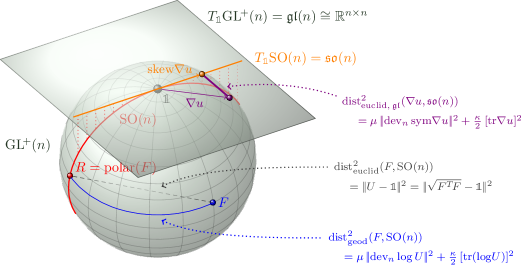
Figure 12: The isotropic Hencky energy of $F$ measures the geodesic distance between $F$ and $\operatorname{SO}(n)$. The linear Euclidean strain measure is obtained as the linearization via the tangent space $\operatorname{\mathfrak{gl}}(n)$ at $\@macros@idbb{1}$.

Remark 3.6.

Using a similar proof, exactly the same result can be shown for the geodesic distance $\operatorname{dist}_{\mathrm{geod,right}}$ induced by the right-$\operatorname{GL}(n)$-invariant, left-$\operatorname{O}(n)$-invariant Riemannian metric [207]

$$g^{\mathrm{right}}_{A}(X,Y)=\langle XA^{-1},YA^{-1}\rangle_{\mu,\mu_{c},\kappa}$$

on $\operatorname{GL}(n)$:

$$\operatorname{dist}_{\mathrm{geod,right}}^{2}(F,\operatorname{SO}(n))=\operatorname{dist}_{\mathrm{geod}}^{2}(F,\operatorname{SO}(n))=\mu\,\lVert\operatorname{dev}_{n}\log U\rVert^{2}+\frac{\kappa}{2}\,[\operatorname{tr}(\log U)]^{2}\,.$$

The right-$\operatorname{GL}(n)$-invariant Riemannian metric can be motivated in a way similar to the left-$\operatorname{GL}(n)$-invariant case: it corresponds to the requirement that the distance between two deformations $F_{1}$ and $F_{2}$ should not depend on the initial shape of $\Omega$, i.e. should not be changed if $\Omega$ is homogeneously deformed beforehand (cf. Figure 13). A similar independence from prior deformations (and so-called “pre-stresses”), called “elastic determinacy” by L. Prandtl [171], was postulated by H. Hencky in the deduction of his elasticity model; cf. [100, p. 618], [146, p. 19] and Section 4.2. $\square$

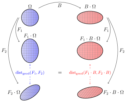
Figure 13: The right-$\operatorname{GL}(n)$-invariance of a distance measure on $\operatorname{GL}(n)$: the distance between two homogeneous deformations $F_{1},F_{2}$ is not changed by a prior homogeneous deformation $B$, i.e. $\operatorname{dist}_{\mathrm{geod}}(F_{1},F_{2})=\operatorname{dist}_{\mathrm{geod}}(F_{1}\cdot B,F_{2}\cdot B)$.

According to Theorem 3.3, the squared geodesic distance between $F$ and $\operatorname{SO}(n)$ with respect to any left-$\operatorname{GL}(n)$-invariant, right-$\operatorname{O}(n)$-invariant Riemannian metric on $\operatorname{GL}(n)$ is the isotropic quadratic Hencky energy

$$W_{\textrm{H}}(F)=\mu\,\lVert\operatorname{dev}_{n}\log U\rVert^{2}+\frac{\kappa}{2}\,[\operatorname{tr}(\log U)]^{2}\,,$$

where the parameters $\mu,\kappa>0$ represent the shear modulus and the bulk modulus, respectively. The Hencky energy function was introduced in 1929 by H. Hencky [101], who derived it from geometrical considerations as well: his deduction was based on a set of axioms including a law of superposition (cf. Section 4.2) for the stress response function [146], an approach previously employed by G. F. Becker [18, 152] in 1893 and later followed in a more general context by H. Richter [176], cf. [177, 175, 178]. A different constitutive model for uniaxial deformations based on logarithmic strain had previously been proposed by Imbert [114] and Hartig [89]. While Ludwik is often credited with the introduction of the uniaxial logarithmic strain, his ubiquitously cited article [124] (which is even referenced by Hencky himself [102, p. 175]) does not provide a systematic introduction of such a strain measure.

While the energy function $W_{\textrm{H}}(F)=\operatorname{dist}_{\mathrm{geod}}^{2}(F,\operatorname{SO}(n))$ already defines a measure of strain as described in Section stress-free reference configuration, we are also interested in characterizing the two terms $\lVert\operatorname{dev}_{n}\log U\rVert$ and $\lvert\operatorname{tr}(\log U)\rvert$ as separate partial strain measures.

Theorem 3.7 (Partial strain measures).

Let

$$\omega_{\mathrm{iso}}(F)\mathrel{\mathchoice{\vbox{\hbox{$\displaystyle:$}}}{\vbox{\hbox{$\textstyle:$}}}{\vbox{\hbox{$\scriptstyle:$}}}{\vbox{\hbox{$\scriptscriptstyle:$}}}{=}}\lVert\operatorname{dev}_{n}\log\sqrt{F^{T}F}\rVert\quad\text{ and }\quad\omega_{\mathrm{vol}}(F)\mathrel{\mathchoice{\vbox{\hbox{$\displaystyle:$}}}{\vbox{\hbox{$\textstyle:$}}}{\vbox{\hbox{$\scriptstyle:$}}}{\vbox{\hbox{$\scriptscriptstyle:$}}}{=}}\lvert\operatorname{tr}(\log\sqrt{F^{T}F})\rvert\,.$$

Then

$$\omega_{\mathrm{iso}}(F) =\operatorname{dist}_{\mathrm{geod,}\operatorname{SL}(n)}\left(\frac{F}{\det F^{1\!/\!\!\;n}},\;\operatorname{SO}(n)\right)$$

and

$$\omega_{\mathrm{vol}}(F) =\sqrt{n}\cdot\operatorname{dist}_{\mathrm{geod,}\,\mathbb{R}^{+}\!\cdot\@macros@idbb{1}}\left((\det F)^{1\!/\!\!\;n}\cdot\@macros@idbb{1},\;\@macros@idbb{1}\right)\,,$$

where the geodesic distances $\operatorname{dist}_{\mathrm{geod,}\operatorname{SL}(n)}$ and $\operatorname{dist}_{\mathrm{geod,}\,\mathbb{R}^{+}\!\cdot\@macros@idbb{1}}$ on the Lie groups $\operatorname{SL}(n)=\{A\in\operatorname{GL}(n)\,|\,\det A=1\}$ and $\mathbb{R}^{+}\cdot\@macros@idbb{1}$ are induced by the canonical left-invariant metric

$$\bar{g}_{A}(X,Y)=\langle A^{-1}X,A^{-1}Y\rangle=\operatorname{tr}(X^{T}A^{-T}A^{-1}Y)\,.$$

Remark 3.8.

Theorem 3.7 states that $\omega_{\mathrm{iso}}$ and $\omega_{\mathrm{vol}}$ appear as natural measures of the isochoric and volumetric strain, respectively: if $F=F_{\mathrm{iso}}\,F_{\mathrm{vol}}$ is decomposed multiplicatively [73] into an isochoric part $F_{\mathrm{iso}}=(\det F)^{-1\!/\!\!\;n}\cdot F$ and a volumetric part $F_{\mathrm{vol}}=(\det F)^{1\!/\!\!\;n}\cdot\@macros@idbb{1}$, then $\omega_{\mathrm{iso}}(F)$ measures the $\operatorname{SL}(n)$-geodesic distance of $F_{\mathrm{iso}}$ to $\operatorname{SO}(n)$, whereas $\frac{1}{\sqrt{n}}\,\omega_{\mathrm{vol}}(F)$ gives the geodesic distance of $F_{\mathrm{vol}}$ to the identity $\@macros@idbb{1}$ in the group $\mathbb{R}^{+}\cdot\@macros@idbb{1}$ of purely volumetric deformations. $\square$

Proof.

First, observe that the canonical left-invariant metrics on $\operatorname{SL}(n)$ and $\mathbb{R}^{+}\cdot\@macros@idbb{1}$ are obtained by choosing $\mu=\mu_{c}=1$ and $\kappa=\frac{2}{n}$ and restricting the corresponding metric $g$ on $\operatorname{GL}^{\!+}(n)$ to the submanifolds $\operatorname{SL}(n)$, $\mathbb{R}^{+}\cdot\@macros@idbb{1}$ and their respective tangent spaces. Then for this choice of parameters, every curve in $\operatorname{SL}(n)$ or $\mathbb{R}^{+}\cdot\@macros@idbb{1}$ is a curve of equal length in $\operatorname{GL}^{\!+}(n)$ with respect to $g$. Since the geodesic distance is defined as the infimal length of connecting curves, this immediately implies

$$\operatorname{dist}_{\mathrm{geod,}\operatorname{SL}(n)}\left(F_{\mathrm{iso}},\;\operatorname{SO}(n)\right)\geq\operatorname{dist}_{\mathrm{geod,}\operatorname{GL}^{\!+}(n)}\left(F_{\mathrm{iso}},\;\operatorname{SO}(n)\right)$$

as well as

$$\operatorname{dist}_{\mathrm{geod,}\,\mathbb{R}^{+}\!\cdot\@macros@idbb{1}}\left(F_{\mathrm{vol}},\;\@macros@idbb{1}\right)\geq\operatorname{dist}_{\mathrm{geod,}\operatorname{GL}^{\!+}(n)}\left(F_{\mathrm{vol}},\;\@macros@idbb{1}\right)\geq\operatorname{dist}_{\mathrm{geod,}\operatorname{GL}^{\!+}(n)}\left(F_{\mathrm{vol}},\;\operatorname{SO}(n)\right)$$

for $F_{\mathrm{iso}}\mathrel{\mathchoice{\vbox{\hbox{$\displaystyle:$}}}{\vbox{\hbox{$\textstyle:$}}}{\vbox{\hbox{$\scriptstyle:$}}}{\vbox{\hbox{$\scriptscriptstyle:$}}}{=}}(\det F)^{-1\!/\!\!\;n}\cdot F$ and $F_{\mathrm{vol}}\mathrel{\mathchoice{\vbox{\hbox{$\displaystyle:$}}}{\vbox{\hbox{$\textstyle:$}}}{\vbox{\hbox{$\scriptstyle:$}}}{\vbox{\hbox{$\scriptscriptstyle:$}}}{=}}(\det F)^{1\!/\!\!\;n}\cdot\@macros@idbb{1}$. We can therefore use Theorem 3.3 to obtain the lower bounds

$$\operatorname{dist}_{\mathrm{geod,}\operatorname{SL}(n)}^{2}\left(F_{\mathrm{iso}},\;\operatorname{SO}(n)\right)$$

$$\geq\operatorname{dist}_{\mathrm{geod,}\operatorname{GL}^{\!+}(n)}^{2}\left(F_{\mathrm{iso}},\;\operatorname{SO}(n)\right)$$

$$=\lVert\operatorname{dev}_{n}\log\left(\sqrt{F_{\mathrm{iso}}^{T}F_{\mathrm{iso}}}\right)\rVert^{2}+\frac{1}{n}\left[\operatorname{tr}\left(\log\sqrt{F_{\mathrm{iso}}^{T}F_{\mathrm{iso}}}\right)\right]^{2}$$

$$=\lVert\log\left(\left(\det\sqrt{F_{\mathrm{iso}}^{T}F_{\mathrm{iso}}}\right)^{-1\!/\!\!\;n}\sqrt{F_{\mathrm{iso}}^{T}F_{\mathrm{iso}}}\right)\rVert^{2}+\frac{1}{n}\,\left[\ln\left(\;\smash{\overbrace{\det\sqrt{F_{\mathrm{iso}}^{T}F_{\mathrm{iso}}}}^{=1}}\vphantom{\det\sqrt{F_{\mathrm{iso}}^{T}F_{\mathrm{iso}}}}\;\right)\right]^{2}$$

$$=\lVert\log\left(\sqrt{F_{\mathrm{iso}}^{T}F_{\mathrm{iso}}}\right)\rVert^{2}=\lVert\log\left((\det F)^{-1\!/\!\!\;n}\sqrt{F^{T}F}\right)\rVert^{2}=\omega_{\mathrm{iso}}^{2}(F)$$ (3.32)

and

$$\operatorname{dist}_{\mathrm{geod,}\,\mathbb{R}^{+}\!\cdot\@macros@idbb{1}}^{2}\left(F_{\mathrm{vol}},\;\@macros@idbb{1}\right) \geq\operatorname{dist}_{\mathrm{geod,}\operatorname{GL}^{\!+}(n)}^{2}\left(F_{\mathrm{vol}},\;\operatorname{SO}(n)\right)$$

$$=\lVert\operatorname{dev}_{n}\log\left(\sqrt{F_{\mathrm{vol}}^{T}F_{\mathrm{vol}}}\right)\rVert^{2}+\frac{1}{n}\,[\operatorname{tr}(\log\left(\sqrt{F_{\mathrm{vol}}^{T}F_{\mathrm{vol}}}\right))]^{2}$$ (3.33)

$$=\lVert\operatorname{dev}_{n}\left(\ln((\det F)^{1\!/\!\!\;n})\cdot\@macros@idbb{1}\right)\rVert^{2}+\frac{1}{n}\,[\ln(\det\left((\det F)^{1\!/\!\!\;n}\cdot\@macros@idbb{1}\right))]^{2}$$

$$=\frac{1}{n}\,[\ln(\det\sqrt{F^{T}F})]^{2}=\frac{1}{n}\,[\operatorname{tr}(\log\sqrt{F^{T}F})]^{2}=\frac{1}{n}\,\omega_{\mathrm{vol}}^{2}(F)\,.$$

To obtain an upper bound on the geodesic distances, we define the two curves

$$\gamma_{\mathrm{iso}}\colon[0,1]\to\operatorname{SL}(n)\,,\quad \gamma_{\mathrm{iso}}(t)=R\,\exp(t\,\operatorname{dev}_{n}\log U)$$

and

$$\gamma_{\mathrm{vol}}\colon[0,1]\to\mathbb{R}^{+}\cdot\@macros@idbb{1}\,,\quad \gamma_{\mathrm{vol}}(t)=e^{\frac{t}{n}\operatorname{tr}(\log U)}\cdot\@macros@idbb{1}\,,$$

where $F=R\,U$ with $R\in\operatorname{SO}(n)$ and $U\in\operatorname{Sym^{+}}(n)$ is the polar decomposition of $F$. Then $\gamma_{\mathrm{iso}}$ connects $(\det F)^{-1\!/\!\!\;n}\cdot F$ to $\operatorname{SO}(n)$:

$$\gamma_{\mathrm{iso}}(0) =R\in\operatorname{SO}(n)\,,$$

$$\gamma_{\mathrm{iso}}(1) =R\,\exp(\operatorname{dev}_{n}\log U) =R\,\exp(\log U-\tfrac{\operatorname{tr}(\log U)}{n}\cdot\@macros@idbb{1})$$

$$=R\,\exp(\log U)\,\exp(-\tfrac{\operatorname{tr}(\log U)}{n}\cdot\@macros@idbb{1})$$

$$=R\,U\,\exp(-\tfrac{\ln\det U}{n}\cdot\@macros@idbb{1})=(\det U)^{-1\!/\!\!\;n}\cdot F=(\det F)^{-1\!/\!\!\;n}\cdot F\,,$$

while $\gamma_{\mathrm{vol}}$ connects $(\det F)^{1\!/\!\!\;n}\cdot\@macros@idbb{1}$ and $\@macros@idbb{1}$:

$$\gamma_{\mathrm{vol}}(0) =\@macros@idbb{1}\,,\quad\gamma_{\mathrm{vol}}(1) =e^{\frac{1}{n}\operatorname{tr}(\log U)}\cdot\@macros@idbb{1}=e^{\frac{1}{n}\ln(\det U)}\cdot\@macros@idbb{1}=(\det U)^{1\!/\!\!\;n}\cdot\@macros@idbb{1}=(\det F)^{1\!/\!\!\;n}\cdot\@macros@idbb{1}\,.$$

The lengths of the curves compute to

$$L(\gamma_{\mathrm{iso}}) =\int_{0}^{1}\lVert\gamma_{\mathrm{iso}}(t)^{-1}{\dot{\gamma}}_{\mathrm{iso}}(t)\rVert\,{\mathrm{d}t}$$ (3.34)

$$=\int_{0}^{1}\lVert(R\,\exp(t\,\operatorname{dev}_{n}\log U))^{-1}\,R\,\exp(t\,\operatorname{dev}_{n}\log U)\,\operatorname{dev}_{n}\log U\rVert\,{\mathrm{d}t}$$

$$=\int_{0}^{1}\lVert\operatorname{dev}_{n}\log U\rVert\,{\mathrm{d}t}=\lVert\operatorname{dev}_{n}\log\sqrt{F^{T}F}\rVert=\omega_{\mathrm{iso}}(F)$$

as well as

$$L(\gamma_{\mathrm{vol}}) =\int_{0}^{1}\lVert\gamma_{\mathrm{vol}}(t)^{-1}{\dot{\gamma}}_{\mathrm{vol}}(t)\rVert\,{\mathrm{d}t}$$ (3.35)

$$=\int_{0}^{1}\lVert(e^{\frac{t}{n}\operatorname{tr}(\log U)}\cdot\@macros@idbb{1})^{-1}\cdot\tfrac{\operatorname{tr}(\log U)}{n}\cdot e^{\frac{t}{n}\operatorname{tr}(\log U)}\cdot\@macros@idbb{1}\rVert\,{\mathrm{d}t}$$

$$=\int_{0}^{1}\lVert\tfrac{\operatorname{tr}(\log U)}{n}\cdot\@macros@idbb{1}\rVert\,{\mathrm{d}t}=\frac{\lvert\operatorname{tr}(\log U)\rvert}{n}\cdot\lVert\@macros@idbb{1}\rVert=\frac{1}{\sqrt{n}}\;\lvert\operatorname{tr}(\log\sqrt{F^{T}F})\rvert=\frac{1}{\sqrt{n}}\;\omega_{\mathrm{vol}}(F)\,,$$

showing that

$$\operatorname{dist}_{\mathrm{geod,}\operatorname{SL}(n)}^{2}\left((\det F)^{-1\!/\!\!\;n}\cdot F,\;\operatorname{SO}(n)\right) \leq L^{2}(\gamma_{\mathrm{iso}})=\omega_{\mathrm{iso}}^{2}(F)$$

and

$$\operatorname{dist}_{\mathrm{geod,}\,\mathbb{R}^{+}\!\cdot\@macros@idbb{1}}^{2}\left((\det F)^{1\!/\!\!\;n}\cdot\@macros@idbb{1},\;\@macros@idbb{1}\right) \leq L^{2}(\gamma_{\mathrm{vol}})=\frac{1}{n}\cdot\omega_{\mathrm{vol}}^{2}(F)\,,$$

which completes the proof. ∎

Remark 3.9.

In addition to the isochoric (distortional) part $F_{\mathrm{iso}}=(\det F)^{-1\!/\!\!\;n}\cdot F$ and the volumetric part $F_{\mathrm{vol}}=(\det F)^{1\!/\!\!\;n}\cdot\@macros@idbb{1}$, we may also consider the cofactor $\operatorname{Cof}F=(\det F)\cdot F^{-T}$ of $F\in\operatorname{GL}^{\!+}(n)$. Theorem 3.3 allows us to directly compute (cf. Appendix A.4) the distance

$$\operatorname{dist}_{\mathrm{geod}}^{2}(\operatorname{Cof}F,\operatorname{SO}(n))=\mu\,\lVert\operatorname{dev}_{n}\log U\rVert^{2}+\frac{\kappa\,(n-1)^{2}}{2}\,[\operatorname{tr}(\log U)]^{2}\,.$$

4 Alternative motivations for the logarithmic strain

4.1 Riemannian geometry applied to $\operatorname{Sym^{+}}(n)$

Extensive work on the use of Lie group theory and differential geometry in continuum mechanics has already been done by Rougée [181, 180, 182, 183], Moakher [137, 139], Bhatia [26] and, more recently, by Fiala [64, 65, 66, 67, 68] (cf. [119, 120, 163, 167, 166]). They all endowed the convex cone $\operatorname{Sym^{+}}(3)$ of positive definite symmetric $(3\times 3)$-tensors with the Riemannian metric

$${\widetilde{g}}_{C}(X,Y)=\operatorname{tr}(C^{-1}XC^{-1}Y)=\langle XC^{-1},C^{-1}Y\rangle=\langle C^{-1\!/\!\!\;2}\,X\,C^{-1\!/\!\!\;2},C^{-1\!/\!\!\;2}\,Y\,C^{-1\!/\!\!\;2}\rangle\,,$$ (4.1)

where $C\in\operatorname{Sym^{+}}(3)$ and $X,Y\in\operatorname{Sym}(3)=T_{C}\operatorname{Sym^{+}}(3)$. Fiala and Rougée deduced a motivation of the logarithmic strain tensor $\log U$ via geodesic curves connecting elements of $\operatorname{Sym^{+}}(n)$. However, their approach differs markedly from our method employed in the previous sections: the manifold $\operatorname{Sym^{+}}(n)$ already corresponds to metric states $C=F^{T}F$, whereas we consider the full set $\operatorname{GL}^{\!+}(n)$ of deformation gradients $F$ (cf. Appendix A.3 and Table 1 in Section 6). This restriction can be viewed as the nonlinear analogue of the a priori restriction to $\varepsilon=\operatorname{sym}\nabla u$ in the linear case, i.e. the nature of the strain measure is not deduced but postulated. Note also that the metric ${\widetilde{g}}$ cannot be obtained by restricting our left-$\operatorname{GL}(3)$-invariant, right-$\operatorname{O}(3)$-invariant metric $g$ to $\operatorname{Sym^{+}}(3)$. Furthermore, while Fiala and Rougée aim to motivate the Hencky strain tensor $\log U$ directly, our focus lies on the strain measures $\omega_{\mathrm{iso}}$, $\omega_{\mathrm{vol}}$ and the isotropic Hencky strain energy $W_{\textrm{H}}$.

The geodesic curves on $\operatorname{Sym^{+}}(n)$ with respect to ${\widetilde{g}}$ are of the simple form

$$\gamma(t)\;=\;C_{1}^{1\!/\!\!\;2}\,\exp(t\cdot C_{1}^{-1\!/\!\!\;2}\,M\,C_{1}^{-1\!/\!\!\;2})\,C_{1}^{1\!/\!\!\;2}$$ (4.2)

with $C_{1}\in\operatorname{Sym^{+}}(n)$ and $M\in\operatorname{Sym}(n)=T_{C_{1}}\!\operatorname{Sym^{+}}(n)$. These geodesics are defined globally, i.e. $\operatorname{Sym^{+}}(n)$ is geodesically complete. Furthermore, for given $C_{1},C_{2}\in\operatorname{Sym^{+}}(n)$, there exists a unique geodesic curve connecting them; this easily follows from the representation formula (4.2) or from the fact that the curvature of $\operatorname{Sym^{+}}(n)$ with ${\widetilde{g}}$ is constant and negative [65, 116, 25]. Note that this implies that, in contrast to $\operatorname{GL}^{\!+}(n)$ with our metric $g$, there are no closed geodesics on $\operatorname{Sym^{+}}(n)$.

An explicit formula for the corresponding geodesic distance was given by Moakher:

$$\operatorname{dist}_{\mathrm{geod,}\operatorname{Sym^{+}}(n)}(C_{1},C_{2})=\lVert\log(C_{2}^{-1\!/\!\!\;2}\,C_{1}\,C_{2}^{-1\!/\!\!\;2})\rVert\,.$$ (4.3)

In the special case $C_{2}=\@macros@idbb{1}$, this distance measure is equal to our geodesic distance on $\operatorname{GL}^{\!+}(n)$ induced by the canonical inner product: Theorem 3.3, applied with parameters $\mu=\mu_{c}=1$ and $\kappa=\frac{2}{n}$ to $R=\@macros@idbb{1}$ and $U=C_{1}$, shows that

$$\operatorname{dist}_{\mathrm{geod,}\operatorname{GL}^{\!+}(n)}(C_{1},\@macros@idbb{1})=\lVert\log C_{1}\rVert=\operatorname{dist}_{\mathrm{geod,}\operatorname{Sym^{+}}(n)}(C_{1},\@macros@idbb{1})\,.$$

More generally, assume that the two metric states $C_{1},C_{2}\in\operatorname{Sym^{+}}(n)$ commute. Then $C_{2}^{-1}C_{1}\in\operatorname{Sym^{+}}(n)$, and the left-$\operatorname{GL}(n)$-invariance of the geodesic distance implies

$$\operatorname{dist}_{\mathrm{geod,}\operatorname{GL}^{\!+}(n)}(C_{1},C_{2}) =\operatorname{dist}_{\mathrm{geod,}\operatorname{GL}^{\!+}(n)}(C_{2}^{-1}C_{1},\@macros@idbb{1})=\lVert\log(C_{2}^{-1}C_{1})\rVert$$

$$=\lVert\log(C_{2}^{-1\!/\!\!\;2}\,C_{2}^{-1\!/\!\!\;2}\,C_{1})\rVert=\lVert\log(C_{2}^{-1\!/\!\!\;2}\,C_{1}\,C_{2}^{-1\!/\!\!\;2})\rVert$$ (4.4)

$$=\operatorname{dist}_{\mathrm{geod,}\operatorname{Sym^{+}}(n)}(C_{1},C_{2})\,.$$

However, since $C_{2}^{-1}C_{1}\notin\operatorname{Sym^{+}}(n)$ in general, this equality does not hold on all of $\operatorname{Sym^{+}}(n)$.

A different approach towards distance functions on the set $\operatorname{Sym^{+}}(n)$ was suggested by Arsigny et al. [8, 9, 7] who, motivated by applications of geodesic and logarithmic distances in diffusion tensor imaging, directly define their Log-Euclidean metric on $\operatorname{Sym^{+}}(n)$ by

$$\operatorname{dist}_{\text{\rm{Log-Euclid}}}(C_{1},C_{2})\mathrel{\mathchoice{\vbox{\hbox{$\displaystyle:$}}}{\vbox{\hbox{$\textstyle:$}}}{\vbox{\hbox{$\scriptstyle:$}}}{\vbox{\hbox{$\scriptscriptstyle:$}}}{=}}\lVert\log C_{1}-\log C_{2}\rVert\,,$$ (4.5)

where $\lVert\,.\,\rVert$ is the Frobenius matrix norm. If $C_{1}$ and $C_{2}$ commute, this distance equals the geodesic distance on $\operatorname{GL}^{\!+}(n)$ as well:

$$\operatorname{dist}_{\mathrm{geod,}\operatorname{GL}^{\!+}(n)}(C_{1},C_{2}) =\lVert\log(C_{2}^{-1}C_{1})\rVert$$

$$=\lVert\log(C_{2}^{-1})+\log(C_{1})\rVert$$ (4.6)

$$=\lVert\log C_{1}-\log C_{2}\rVert=\operatorname{dist}_{\text{\rm{Log-Euclid}}}(C_{1},C_{2})\,,$$

where equality in (4.6) holds due to the fact that $C_{1}$ and $C_{2}^{-1}$ commute. Again, this equality does not hold for arbitrary $C_{1}$ and $C_{2}$.

Using a similar Riemannian metric, geodesic distance measures can also be applied to the set of positive definite symmetric fourth-order elasticity tensors, which can be identified with $\operatorname{Sym^{+}}(6)$. Norris and Moakher applied such a distance function in order to find an isotropic elasticity tensor $\mathbb{C}\colon\operatorname{Sym}(3)\to\operatorname{Sym}(3)$ which best approximates a given anisotropic tensor [138, 157].

The connection between geodesic distances on the metric states in $\operatorname{Sym^{+}}(n)$ and logarithmic distance measures was also investigated extensively by the late Albert Tarantola [197], a lifelong advocate of logarithmic measures in physics. In his view [197, 4.3.1], “…the configuration space is the Lie group $\operatorname{GL}^{\!+}(3)$, and the only possible measure of strain (as the geodesics of the space) is logarithmic.”

4.2 Further mechanical motivations for the quadratic isotropic Hencky model based on logarithmic strain tensors

“At the foundation of all elastic theories lies the definition of strain, and before introducing a new law of elasticity we must explain how finite strain is to be measured.”

Heinrich Hencky: The elastic behavior of vulcanized rubber [103].    
Apart from the geometric considerations laid out in the previous sections, the Hencky strain tensor $E_{0}=\log U$ can be characterized via a number of unique properties.

For example, the Hencky strain is the only strain tensor (for a suitably narrow definition, cf. [152]) that satisfies the law of superposition for coaxial deformations:

$$E_{0}(U_{1}\cdot U_{2})=E_{0}(U_{1})+E_{0}(U_{2})$$ (4.7)

for all coaxial stretches $U_{1}$ and $U_{2}$, i.e. $U_{1},U_{2}\in\operatorname{Sym^{+}}(n)$ such that $U_{1}\cdot U_{2}=U_{2}\cdot U_{1}$. This characterization was used by Heinrich Hencky [196, 97, 102, 103] in his original introduction of the logarithmic strain tensor [99, 101, 100, 146] and, indeed much earlier, by the geologist George Ferdinand Becker [133], who postulated a similar law of superposition in order to deduce a logarithmic constitutive law of nonlinear elasticity [18, 152] (cf. Appendix A.2).

In the case $n=1$, this superposition principle simply amounts to the fact that the logarithm function $f=\log$ satisfies Cauchy’s [40] well-known functional equation

$$f(\lambda_{1}\cdot\lambda_{2})=f(\lambda_{1})+f(\lambda_{2})\,,$$ (4.8)

i.e. that the logarithm is an isomorphism between the multiplicative group $(\mathbb{R}_{+},\cdot)$ and the additive group $(\mathbb{R},+)$. This means that for a sequence of incremental one-dimensional deformations, the logarithmic strains $\mathrm{e}_{\mathrm{log}}^{i}$ can be added in order to obtain the total logarithmic strain $\mathrm{e}_{\mathrm{log}}^{\mathrm{tot}}$ of the composed deformation [72]:

$$\mathrm{e}_{\mathrm{log}}^{1}+\mathrm{e}_{\mathrm{log}}^{2}+\ldots+\mathrm{e}_{\mathrm{log}}^{n}=\log\frac{L_{1}}{L_{0}}+\log\frac{L_{2}}{L_{1}}+\ldots+\log\frac{L_{n}}{L_{n-1}}=\log\frac{L_{n}}{L_{0}}=\mathrm{e}_{\mathrm{log}}^{\mathrm{tot}}\,,$$

where $L_{i}$ denotes the length of the (one-dimensional) body after the $i$-th elongation. This property uniquely characterizes the logarithmic strain $\mathrm{e}_{\mathrm{log}}$ among all differentiable one-dimensional strain mappings $\mathrm{e}\colon\mathbb{R}^{+}\to\mathbb{R}$ with $\mathrm{e}^{\prime}(1)=1$.

Since purely volumetric deformations of the form $\lambda\cdot\@macros@idbb{1}$ with $\lambda>0$ are coaxial to every stretch $U\in\operatorname{Sym^{+}}(n)$, the decomposition property (4.7) allows for a simple additive volumetric-isochoric split of the Hencky strain tensor [176]:

$$\log U=\,\log\bigg{[}\underbrace{\frac{U}{(\det U)^{1\!/\!\!\;n}}}_{\text{isochoric}}\>\cdot\>\underbrace{\vphantom{\frac{U}{(\det U)^{1\!/\!\!\;n}}}(\det U)^{1\!/\!\!\;n}\cdot\@macros@idbb{1}}_{\text{volumetric}}\bigg{]} =\,\log\bigg{[}\frac{U}{(\det U)^{1\!/\!\!\;n}}\bigg{]}\>+\>\log\Big{[}(\det U)^{1\!/\!\!\;n}\cdot\@macros@idbb{1}\Big{]}$$

$$=\,\underbrace{\vphantom{\frac{U}{(\det U)^{1\!/\!\!\;n}}}\operatorname{dev}_{n}\log U}_{\text{isochoric}}\>+\>\underbrace{\vphantom{\frac{U}{(\det U)^{1\!/\!\!\;n}}}\frac{1}{n}\operatorname{tr}(\log U)\cdot\@macros@idbb{1}}_{\text{volumetric}}\,.$$

In particular, the incompressibility condition $\det F=1$ can be easily expressed as $\operatorname{tr}(\log U)=0$ in terms of the logarithmic strain tensor.

4.2.1 From Truesdell’s hypoelasticity to Hencky’s hyperelastic model

As indicated in Section 1.1, the quadratic Hencky energy is also of great importance to the concept of hypoelasticity [83, Chapter IX]. It was found that the Truesdell equation [199, 201, 200, 76]

$$\frac{\mathrm{d}}{\mathrm{d}t}^{\!\!\square}[\tau]=2\,\mu\,D+\lambda\,\operatorname{tr}(D)\cdot\@macros@idbb{1}\,,\qquad D=\operatorname{sym}(\dot{F}\,F^{-1})\,,$$ (4.9)

with constant Lamé coefficients $\mu,\lambda>0$, under the assumption that the stress rate $\frac{\mathrm{d}}{\mathrm{d}t}^{\!\!\square}$ is objective and corotational, is satisfied if and only if $\frac{\mathrm{d}}{\mathrm{d}t}^{\!\!\square}$ is the so-called logarithmic corotational rate $\frac{\mathrm{d}}{\mathrm{d}t}^{\!\!\mathrm{log}}$ and $\tau=2\,\mu\,\log V+\lambda\,\operatorname{tr}(\log V)\cdot\@macros@idbb{1}$ [211, 209, 158, 172, 173, 212, 213, 214], i.e. if and only if the hypoelastic model is exactly Hencky’s hyperelastic constitutive model. Here, $\tau=\det F\cdot\sigma(V)$ denotes the Kirchhoff stress tensor and $D$ is the unique rate of stretching tensor (i.e. the symmetric part of the velocity gradient in the spatial setting). A rate $\frac{\mathrm{d}}{\mathrm{d}t}^{\!\!\square}$ is called corotational if it is of the special form

$$\frac{\mathrm{d}}{\mathrm{d}t}^{\!\!\square}[X]=\dot{X}-\Omega X+X\Omega\quad\text{ with $\Omega\in\operatorname{\mathfrak{so}}(3)$}\,,$$ (4.10)

which means that the rate is computed with respect to a frame that is rotated. This extra rate of rotation is defined only by the underlying spins of the problem. Upon specialisation, for $\mu=1$, $\lambda=0$ we obtain [34, eq. 71]

$$\frac{\mathrm{d}}{\mathrm{d}t}^{\!\!\mathrm{log}}[\log V]=D$$

as the unique solution to (4.9) with a corotational rate. Note that this characterization of the spatial logarithmic strain tensor $\log V$ is by no means exceptional. For example, it is well known that [90, p. 49, Theorem 1.8] (cf. [35])

$$\frac{\mathrm{d}}{\mathrm{d}t}^{\!\!\vartriangle}[A]=\dot{A}+L^{T}A+AL=D\,,$$

where $A={\widehat{E}}_{-1}=\frac{1}{2}(\@macros@idbb{1}-B^{-1})$ is the spatial Almansi strain tensor and $\frac{\mathrm{d}}{\mathrm{d}t}^{\!\!\vartriangle}$ is the upper Oldroyd rate (as defined in (4.14)).

The quadratic Hencky model

$$\tau=2\,\mu\,\log V+\lambda\,\operatorname{tr}(\log V)\cdot\@macros@idbb{1}=D_{\log V}W_{\textrm{H}}(\log V)$$ (4.11)

was generalized in Hill’s generalized linear elasticity laws [108, eq. (2.69)]

$$T_{r}=2\,\mu\,E_{r}+\lambda\,\operatorname{tr}(E_{r})\cdot\@macros@idbb{1}$$ (4.12)

with work-conjugate pairs $(T_{r},E_{r})$ based on the Lagrangian strain measures given in (1.3); cf. Appendix A.2 for examples. The concept of work-conjugacy was introduced by Hill [106] via an invariance requirement; the spatial stress power must be equal to its Lagrangian counterpart:

$$\det F\cdot\langle\sigma,D\rangle=\langle T_{r},\dot{E}_{r}\rangle\,,$$ (work-conjugacy)

by means of which a material stress tensor is uniquely linked to its (material rate) conjugate strain tensor. Hence it generalizes the virtual work principle and is the foundation of derived methods like the finite element method.

For the case of isotropic materials, Hill [106, p. 242] (cf. [109]) shows by spectral decomposition techniques that the work-conjugate stress to $\log U$ is the back-rotated Cauchy stress $\sigma$ multiplied by $\det F$, hence $\langle\sigma,D\rangle=\langle R^{T}\,\sigma\,R,\;\frac{\mathrm{d}}{\mathrm{d}t}\log U\rangle$, which is a generalization of Hill’s earlier work [106, 108]. Sansour [185] additionally found that the Eshelby-like stress tensor $\Sigma=CS_{2}$ is equally conjugate to $\log U$; here, $S_{2}$ denotes the second Piola-Kirchhoff stress tensor. For anisotropy, however, the conjugate stress exists but follows a much more complex format than for isotropy [109]. The logarithm of the left stretch $\log V$ in contrast exhibits a work conjugate stress tensor only for isotropic materials, namely the Kirchhoff stress tensor $\tau=\det F\cdot\sigma$ [162, 109].

While hyperelasticity in its potential format avoids rate equations, the use of stress rates (i.e. stress increments in time) may be useful for the description of inelastic material behavior at finite strains. Since the material time derivative of an Eulerian stress tensor is not objective, rates for a tensor $X$ were developed, like the (objective and corotational) Zaremba-Jaumann rate

$$\frac{\mathrm{d}}{\mathrm{d}t}^{\!\!\circ}[X]=\dot{X}-WX+XW\,,\qquad W=\mathop{\mathrm{skew}}\nolimits L\,,\quad L=\dot{F}F^{-1}\,,$$ (4.13)

or the (objective but not corotational) lower and upper Oldroyd rates

$$\frac{\mathrm{d}}{\mathrm{d}t}^{\!\!\triangledown}[X]=\dot{X}+L^{T}X+XL\qquad\text{and}\qquad\frac{\mathrm{d}}{\mathrm{d}t}^{\!\!\vartriangle}[X]=\dot{X}-LX-XL^{T}\,,$$ (4.14)

to name but a few (cf. [90, Section 1.7] and [186]). Which one of these or the great number of other objective rates should be used seems to be rather a matter of taste, hence of arbitrariness or heuristics, but not a matter of theory.

The concept of dual variables as introduced by Tsakmakis and Haupt in [91] into continuum mechanics overcame the arbitrariness of the chosen rate in that it uniquely connects a particular (objective) strain rate to a stress tensor and, analogously, a stress rate to a strain tensor. The rational rule is that, when stress and strain tensors operate on configurations other than the reference configurations, the physically significant scalar products $\langle S_{2},\dot{E}_{1}\rangle$, $\langle\dot{S}_{2},E_{1}\rangle$, $\langle S_{2},E_{1}\rangle$ and $\langle{\dot{S}}_{2},\dot{E}_{1}\rangle$ (with the second Piola-Kirchhoff stress tensor $S_{2}$ and its work-conjugate Green strain tensor $E_{1}$) must remain invariant, see [91, 90].

4.2.2 Advantageous properties of the quadratic Hencky energy

For modelling elastic material behavior there is no theoretical reason to prefer one strain tensor over another one, and the same is true for stress tensors. As discussed in Section 1.1, stress and strain are immaterial. Primary experimental data (forces, displacements) in material testing are sufficient to calculate any strain tensor and any stress tensor and to display any combination thereof in stress-strain curves, while only work-conjugate pairs are physically meaningful.

However, for modelling finite-strain elasticity, the quadratic Hencky model

$$W_{\textrm{H}} =\mu\,\lVert\operatorname{dev}_{n}\log V\rVert^{2}+\frac{\kappa}{2}\,[\operatorname{tr}(\log V)]^{2}=\mu\,\lVert\operatorname{dev}_{n}\log U\rVert^{2}+\frac{\kappa}{2}\,[\operatorname{tr}(\log U)]^{2}\,,$$

$$\tau =2\,\mu\,\operatorname{dev}_{n}\log V+\kappa\,\operatorname{tr}(\log V)\,\@macros@idbb{1}\,,$$ (4.15)

exhibits a number of unique, favorable properties, including its functional simplicity and its dependency on only two material parameters $\mu$ and $\kappa$ that are determined in the infinitesimal strain regime and remain constant over the entire strain range. In view of the linear dependency of stress from logarithmic strain in (4.15), it is obvious that any nonlinearity in the stress-strain curves can only be captured in Hencky’s model by virtue of the nonlinearity in the strain tensor itself. There is a surprisingly large number of different materials, where Hencky’s elasticity relation provides a very good fit to experimental stress-strain data, which is true for different length scales and strain regimes. In the following we substantiate this claim with some examples.

Nonlinear elasticity on macroscopic scales for a variety of materials.  Anand [3, 4] has shown that the Hencky model is in good agreement with experiments on a wide class of materials, e.g. vulcanized natural rubber, for principal stretches between $0.7$ and $1.3$. More precisely, this refers to the characteristic that in tensile deformation the stiffness becomes increasingly smaller compared with the stiffness at zero strain, while for compressive deformation the stiffness becomes increasingly larger.

Nonlinear elasticity in the very small strain regime.  We mention in passing that a qualitatively similar dependency of material stiffness on the sign of the strain has been made much earlier in the regime of extremely small strains ($10^{-6}$–$10^{-3}$). In Hartig’s law [89] from 1893 this dependency was expressed as $\frac{\mathrm{d}\sigma}{\mathrm{d}\varepsilon}=E^{0}+b\,\sigma$, where $E^{0}$ is the elasticity modulus at zero stress and $b<0$ is a dimensionless constant, cf. the book of Bell [19] and [126] in the context of linear elasticity with initial stress. Hartig also observed that the stress-stretch relation should have negative curvature in the vicinity of the identity, as shown in Figure 14.

Crystalline elasticity on the nanoscale.  Quite in contrast to the strictly stress-based continuum constitutive modelling, atomistic theories are based on a concept of interatomic forces. These forces are derived from potentials $\mathcal{V}$ according to the potential relation $f_{a}=-\partial_{x_{a}}\mathcal{V}$, which endows the model with a variational structure. A further discussion of hybrid, atomistic-continuum coupling can be found in [60]. Thereby the discreteness of matter at the nanoscale and the nonlocality of atomic interactions are inherently captured. Here, atomistic stress is neither a constitutive agency nor does it enter a balance equation. Instead, it optionally can be calculated following the virial stress theorem [195, Chapter 8] to illustrate the state of the system.

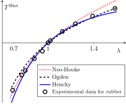
Figure 14: The Biot stress $T^{\mathrm{Biot}}$ corresponding to uniaxial stretches by factor $\lambda$ of incompressible materials fitted to experimental measurements by Jones and Treloar [115]. The curvature in $\lambda=1$ suggests negative third order constants ($b<0$), which has also been postulated by Grioli [84, eq. (32)].

With their analyses in [53] and [54], Dłużewski and coworkers aim to link the atomistic world to the macroscopic world of continuum mechanics. They search for the “best” strain measure with a view towards crystalline elasticity on the nanoscale. The authors consider the deformation of a crystal structure and compare the atomistic and continuum approaches. Atomistic calculations are made using the Stillinger-Weber potential. The stress-strain behaviour of the best-known anisotropic hyperelastic models are compared with the behaviour of the atomistic one in the uniaxial deformation test. The result is that the anisotropic energy based on the Hencky strain energy $\frac{1}{2}\,\langle\mathbb{C}.\log U,\log U\rangle$, where $\mathbb{C}$ is the anisotropic elasticity tensor from linear elasticity, gives the best fit to atomistic simulations. More in detail, this best fit manifests itself in the observation that for considerable compression (up to $\approx 20\%$) the material stiffness is larger than the reference stiffness at zero strain, and for considerable tension (up to $\approx 20\%$) it is smaller than the zero-strain stiffness, again in good agreement with the atomistic result. This is also corroborated by comparing tabulated experimentally determined third order elastic constants [53].

Elastic energy potentials based on logarithmic strain have also recently been motivated via molecular dynamics simulations [93] by Henann and Anand [94].

5 Applications and ongoing research

5.1 The exponentiated Hencky energy

As indicated in Section stress-free reference configuration and shown in Sections 2.1 and 3, strain measures are closely connected to isotropic energy functions in nonlinear hyperelasticity: similarly to how the linear elastic energy may be obtained as the square of the Euclidean distance of $\nabla u$ to $\operatorname{\mathfrak{so}}(n)$, the nonlinear quadratic Hencky strain energy is the squared Riemannian distance of $\nabla\varphi$ to $\operatorname{SO}(n)$. For the partial strain measures $\omega_{\mathrm{iso}}(F)=\lVert\operatorname{dev}_{n}\log\sqrt{F^{T}F}\rVert$ and $\omega_{\mathrm{vol}}(F)=\lvert\operatorname{tr}(\log\sqrt{F^{T}F})\rvert$ defined in Theorem 3.7, the Hencky strain energy $W_{\textrm{H}}$ can be expressed as

$$W_{\textrm{H}}(F)=\mu\,\omega_{\mathrm{iso}}^{2}(F)+\frac{\kappa}{2}\,\omega_{\mathrm{vol}}^{2}(F)\,.$$ (5.1)

However, it is not at all obvious why this weighted squared sum should be viewed as the “canonical” energy associated with the geodesic strain measures: while it is reasonable to view the elastic energy as a quantity depending on some strain measure alone, the specific form of this dependence must not be determined by purely geometric deductions, but must take into account physical constraints as well as empirical observations.

For a large number of materials, the Hencky energy does indeed provide a very accurate model up to moderately large elastic deformations [3, 4], i.e. up to stretches of about $40\%$, with only two constant material parameters which can be easily determined in the small strain range. For very large strains, however, the subquadratic growth of the Hencky energy in tension is no longer in agreement with empirical measurements. In a series of articles [154, 155, 153, 80], Neff et al. have therefore introduced the exponentiated Hencky energy

$$W_{\textrm{eH}}(F)\; =\;\frac{\mu}{k}\,e^{k\,\omega_{\mathrm{iso}}^{2}(F)}+\frac{\kappa}{2\hat{k}}\,e^{\hat{k}\,\omega_{\mathrm{vol}}^{2}(F)}\;=\;\frac{\mu}{k}\,e^{k\,\|\operatorname{dev}_{n}\log{U}\|^{2}}+\frac{\kappa}{2\hat{k}}\,e^{\hat{k}\,[\operatorname{tr}(\log U)]^{2}}$$ (5.2)

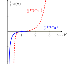
Figure 15: The equation of state (EOS), i.e. the trace of the Cauchy stress corresponding to a purely volumetric deformation (cf. [168]), for the quadratic and the exponentiated Hencky model (with parameter ${\widehat{k}}=4$).

with additional dimensionless material parameters $k\geq\frac{1}{4}$ and ${\widehat{k}}\geq\frac{1}{8}$, which for all values of $k,{\widehat{k}}$ approximates $W_{\textrm{H}}$ for deformation gradients $F$ sufficiently close to the identity $\@macros@idbb{1}$, but shows a vastly different behaviour for $\lVert F\rVert\to\infty$, cf. Figure 16.

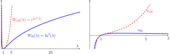
Figure 16: The one-dimensional Hencky energy $W_{\textrm{H}}$ compared to the exponentiated Hencky energy $W_{\textrm{eH}}$ and the corresponding Cauchy stresses $\sigma_{\mathrm{H}}$, $\sigma_{\mathrm{eH}}$ for very large uniaxial stretches $\lambda$. Observe the non-convexity of $W_{\textrm{H}}$ and the non-invertibility of $\sigma_{H}$.

The exponentiated Hencky energy has many advantageous properties over the classical quadratic Hencky energy; for example, $W_{\textrm{eH}}$ is coercive on all Sobolev spaces $W^{1,p}$ for $1\leq p<\infty$, thus cavitation is excluded [12, 143]. In the planar case $n=2$, $W_{\textrm{eH}}$ is also polyconvex [155, 80] and thus Legendre-Hadamard-elliptic [10], whereas the classical Hencky energy is not even LH-elliptic (rank-one convex) outside a moderately large neighbourhood of $\@macros@idbb{1}$ [36, 144] (see also [113], where the loss of ellipticity for energies of the form $\lVert\operatorname{dev}_{3}\log U\rVert^{\beta}$ with hardening index $0<\beta<1$ are investigated). Therefore, many results guaranteeing the existence of energy-minimizing deformations for a variety of boundary value problems can be applied directly to $W_{\textrm{eH}}$ for $n=2$.

Furthermore, $W_{\textrm{eH}}$ satisfies a number of constitutive inequalities [154] such as the Baker-Ericksen inequality [127], the pressure-compression inequality and the tension-extension inequality as well as Hill’s inequality [107, 160, 161], which is equivalent to the convexity of the elastic energy with respect to the logarithmic strain tensor [192].

Moreover, for $W_{\textrm{eH}}$, the Cauchy-stress-stretch relation $V\mapsto\sigma_{\mathrm{eH}}(V)$ is invertible (a property hitherto unknown for other hyperelastic formulations) and pure Cauchy shear stress corresponds to pure shear strain, as is the case in linear elasticity [154]. The physical meaning of Poisson’s ratio [169, 79] $\nu=\frac{3\kappa-2\mu}{2(3\kappa+\mu)}$ is also similar to the linear case; for example, $\nu=\frac{1}{2}$ directly corresponds to incompressibility of the material and $\nu=0$ implies that no lateral extension or contraction occurs in uniaxial tensions tests.

5.2 Related geodesic distances

The logarithmic distance measures obtained in Theorems 3.3 and 3.7 show a strong similarity to other geodesic distance measures on Lie groups. For example, consider the special orthogonal group $\operatorname{SO}(n)$ endowed with the canonical bi-invariant Riemannian metric

$$\hat{g}_{Q}(X,Y)=\langle Q^{T}X,Q^{T}Y\rangle=\langle X,Y\rangle$$

for $Q\in\operatorname{SO}(n)$ and $X,Y\in T_{Q}\operatorname{SO}(n)=Q\cdot\operatorname{\mathfrak{so}}(n)$. Then the geodesic exponential at $\@macros@idbb{1}\in\operatorname{SO}(n)$ is given by the matrix exponential on the Lie algebra $\operatorname{\mathfrak{so}}(n)$, i.e. all geodesic curves are one-parameter groups of the form

$$\widehat{\gamma}(t)=Q\cdot\exp(t\,A)$$

with $Q\in\operatorname{SO}(n)$ and $A\in\operatorname{\mathfrak{so}}(n)$ (cf. [136]). It is easy to show that the geodesic distance between $Q,R\in\operatorname{SO}(n)$ with respect to this metric is given by

$$\operatorname{dist}_{\mathrm{geod,}\operatorname{SO}(n)}(Q,R)=\lVert\log(Q^{T}R)\rVert\,,$$

where $\lVert\,.\,\rVert$ is the Frobenius matrix norm and $\log\colon\operatorname{SO}(n)\to\operatorname{\mathfrak{so}}(n)$ denotes the principal matrix logarithm on $\operatorname{SO}(n)$, which is uniquely defined by the equality $\exp(\log Q)=Q$ and the requirement $\lambda_{i}(\log Q)\in(-\pi,\pi]$ for all $Q\in\operatorname{SO}(n)$ and all eigenvalues $\lambda_{i}(\log Q)$.

This result can be extended to the geodesic distance on the conformal special orthogonal group $\operatorname{CSO}(n)$ consisting of all angle-preserving linear mappings:

$$\operatorname{CSO}(n)\mathrel{\mathchoice{\vbox{\hbox{$\displaystyle:$}}}{\vbox{\hbox{$\textstyle:$}}}{\vbox{\hbox{$\scriptstyle:$}}}{\vbox{\hbox{$\scriptscriptstyle:$}}}{=}}\{c\cdot Q\;|\;c>0\,,\;Q\in\operatorname{SO}(n)\}\,,$$

where the bi-invariant metric $g_{\operatorname{CSO}(n)}$ is given by the canonical inner product:

$$g_{A}^{\operatorname{CSO}(n)}(X,Y)=\langle A^{-1}X,A^{-1}Y\rangle\,.$$ (5.3)

Then

$$\operatorname{dist}_{\mathrm{geod,}\operatorname{CSO}(n)}^{2}(c\cdot Q,d\cdot R)=\lVert\log(Q^{T}R)\rVert^{2}+\frac{1}{n}\left[\ln\left(\frac{c}{d}\right)\right]^{2}\,,$$

where $\log$ again denotes the principal matrix logarithm on $\operatorname{SO}(n)$. Note that the punctured complex plane $\mathbb{C}\setminus\{0\}$ can be identified with $\operatorname{CSO}(2)$ via the mapping

$$z=a+i\,b\quad\mapsto\quad Z\in\operatorname{CSO}(2)=\left\{\begin{pmatrix}a&b\\ -b&a\end{pmatrix}\,\bigg{|}\;a^{2}+b^{2}\neq 0\right\}\,.$$

5.3 Outlook

While first applications of the exponentiated Hencky energy, which is based on the partial strain measures $\omega_{\mathrm{iso}},\,\omega_{\mathrm{vol}}$ introduced here, show promising results, including an accurate modelling of so-called tire-derived material [140], a more thorough fitting of the new parameter set to experimental data is necessary in order to assess the range of applicability of $W_{\textrm{eH}}$ towards elastic materials like vulcanized rubber. A different formulation in terms of the partial strain measures $\omega_{\mathrm{iso}}$ and $\omega_{\mathrm{vol}}$, i.e. an energy function of the form

$$W(F)\;=\;\Psi(\omega_{\mathrm{iso}}(F),\omega_{\mathrm{vol}}(F))\;=\;\Psi(\lVert\operatorname{dev}_{3}\log U\rVert,\,\lvert\operatorname{tr}(\log U)\rvert)$$ (5.4)

with $\Psi\colon[0,\infty)^{2}\to[0,\infty)$, might even prove to be polyconvex in the three-dimensional case. The main open problem of finding a polyconvex (or rank-one convex) isochoric energy function $F\mapsto\widetilde{\Psi}(\lVert\operatorname{dev}_{3}\log U\rVert)$ has also been considered by Sendova and Walton [189]. Note that while every isotropic elastic energy $W$ can be expressed as $W(F)=h(K_{1},K_{2},K_{3})$ with Criscione’s invariants [46, 45, 51, 208]

$$K_{1}=\operatorname{tr}(\log U)\,,\qquad K_{2}=\lVert\operatorname{dev}_{3}\log U\rVert\qquad\text{ and }\qquad K_{3}=\det\left(\frac{\operatorname{dev}_{3}\log U}{\lVert\operatorname{dev}_{3}\log U\rVert}\right)\,,$$ (5.5)

not every elastic energy has a representation of the form (5.4); for example, (5.4) implies the tension-compression symmetry $W(F)=W(F^{-1})$, which is not necessarily satisfied by energy functions in general. In terms of the Shield transformation [191, 39]

$$W^{*}(F)\mathrel{\mathchoice{\vbox{\hbox{$\displaystyle:$}}}{\vbox{\hbox{$\textstyle:$}}}{\vbox{\hbox{$\scriptstyle:$}}}{\vbox{\hbox{$\scriptscriptstyle:$}}}{=}}\det F\cdot W(F^{-1})\,,$$

the tension-compression symmetry amounts to the requirement $\frac{1}{\det F}\,W^{*}(F)=W(F)$ or, for incompressible materials, $W^{*}(F)=W(F)$. Moreover, under the assumption of incompressibility, the symmetry can be immediately extended to arbitrary deformations $\varphi\colon\Omega\to\varphi(\Omega)$ and $\varphi^{-1}\colon\varphi(\Omega)\to\Omega$: if $\det\nabla\varphi\equiv 1$, we can apply the substitution rule to find

$$\int_{\varphi(\Omega)}W(\nabla(\varphi^{-1})(x))\,{\mathrm{d}x} =\int_{\Omega}W(\nabla(\varphi^{-1})(\varphi(x)))\cdot\lvert\det\nabla\varphi(x)\rvert\,{\mathrm{d}x}$$

$$=\int_{\Omega}W(\nabla\varphi(x)^{-1})\,{\mathrm{d}x}=\int_{\Omega}W(\nabla\varphi(x))\,{\mathrm{d}x}$$

if $W(F^{-1})=W(F)$ for all $F\in\operatorname{SL}(n)$, thus the total energies of the deformations $\varphi,\varphi^{-1}$ are equal, cf. Figure 17.

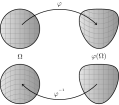
Figure 17: The tension-compression symmetry for incompressible materials: if $\det\nabla\varphi\equiv 1$ and $W(F^{-1})=W(F)$ for all $F\in\operatorname{SL}(n)$, then $\int_{\Omega}W(\nabla\varphi(x))\,{\mathrm{d}x}=\int_{\varphi(\Omega)}W(\nabla(\varphi^{-1})(x))\,{\mathrm{d}x}$.

Since the function

$$F\mapsto e^{\lVert\operatorname{dev}_{2}\log U\rVert^{2}}=e^{\operatorname{dist}_{\mathrm{geod,}\operatorname{SL}(2)}^{2}\left(\frac{F}{\det F^{1\!/\!\!\;2}},\;\operatorname{SO}(2)\right)}$$

in planar elasticity is polyconvex [155, 80], it stands to reason that a similar formulation in the three-dimensional case might prove to be polyconvex as well. A first step towards finding such an energy is to identify where the function $W$ with

$$W(F)=e^{\lVert\operatorname{dev}_{3}\log U\rVert^{2}}=e^{\operatorname{dist}_{\mathrm{geod,}\operatorname{SL}(3)}^{2}\left(\frac{F}{\det F^{1\!/\!\!\;3}},\;\operatorname{SO}(3)\right)}\,,$$ (5.6)

which is not rank-one convex [154], loses its ellipticity properties. For that purpose, it may be useful to consider the quasiconvex hull of $W$. There already are a number of promising results for similar energy functions; for example, the quasiconvex hull of the mapping

$$F\mapsto\operatorname{dist}_{\mathrm{Euclid}}^{2}(F,\operatorname{SO}(2))=\lVert U-\@macros@idbb{1}\rVert^{2}$$

can be explicitly computed [194, 56, 57], and the quasiconvex hull of the similar Saint-Venant-Kirchhoff energy $W_{\textrm{SVK}}(F)=\frac{\mu}{4}\,\lVert C-\@macros@idbb{1}\rVert^{2}+\frac{\lambda}{8}\,[\operatorname{tr}(C-\@macros@idbb{1})]^{2}$ has been given by Le Dret and Raoult [121]. For the mappings

$$F\mapsto\operatorname{dist}_{\mathrm{Euclid}}^{2}(F,\operatorname{SO}(3))\quad\text{ or }\quad F\mapsto\operatorname{dist}_{\mathrm{geod}}^{2}(F,\operatorname{SO}(n))$$

with $n\geq 2$, however, no explicit representation of the quasiconvex hull is yet known, although it has been shown that both expressions are not rank-one convex [24].

It might also be of interest to calculate the geodesic distance $\operatorname{dist}_{\mathrm{geod}}(A,B)$ for a larger class of matrices $A,B\in\operatorname{GL}^{\!+}(n)$: although Theorem 3.3 allows us to explicitly compute the distance $\operatorname{dist}_{\mathrm{geod}}(\@macros@idbb{1},P)$ for $P\in\operatorname{Sym^{+}}(n)$ and local results are available for certain special cases [129], it is an open question whether there is a general formula for the distance $\operatorname{dist}_{\mathrm{geod,}\operatorname{GL}^{\!+}(n)}(Q,R)$ between arbitrary rotations $R,Q\in\operatorname{SO}(n)$ for all parameters $\mu,\mu_{c},\kappa>0$. Since restricting our left-$\operatorname{GL}(n)$-invariant, right-$\operatorname{O}(n)$-invariant metric on $\operatorname{GL}(n)$ to $\operatorname{SO}(n)$ yields a multiple of the canonical bi-$\operatorname{SO}(n)$-invariant metric on $\operatorname{SO}(n)$, we can compute

$$\operatorname{dist}_{\mathrm{geod,}\operatorname{GL}^{\!+}(n)}^{2}(Q,R)=\mu_{c}\cdot\operatorname{dist}_{\mathrm{geod,}\operatorname{SO}(n)}^{2}(Q,R)=\mu_{c}\,\lVert\log(Q^{T}R)\rVert^{2}$$

if for all $Q,R\in\operatorname{SO}(n)$ a shortest geodesic in $\operatorname{GL}^{\!+}(n)$ connecting $Q$ and $R$ is already contained within $\operatorname{SO}(n)$, cf. Figure 18. However, whether this is the case depends on the chosen parameters $\mu,\mu_{c}$; a general closed-form solution for $\operatorname{dist}_{\mathrm{geod,}\operatorname{GL}^{\!+}(n)}$ on $\operatorname{SO}(n)$ is therefore not yet known [128].

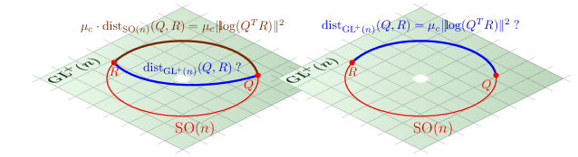
Figure 18: If $\operatorname{SO}(n)$ contains a length minimizing geodesic connecting $Q,R\in\operatorname{SO}(n)$ with respect to our left-$\operatorname{GL}(n)$-invariant, right-$\operatorname{O}(n)$-invariant metric $g$ on $\operatorname{GL}(n)$, then the $\operatorname{GL}^{\!+}(n)$-geodesic distance between $Q$ and $R$ is equal to the well-known $\operatorname{SO}(n)$-geodesic distance $\mu_{c}\,\lVert\log(Q^{T}R)\rVert^{2}$.

Moreover, it is not known whether our result can be generalized to anisotropic Riemannian metrics, i.e. if the geodesic distance to $\operatorname{SO}(n)$ can be explicitly computed for a larger class of left-$\operatorname{GL}(n)$-invariant Riemannian metrics which are not necessarily right-$\operatorname{O}(n)$-invariant. A result in this direction would have immediate impact on the modelling of finite strain anisotropic elasticity [14, 188, 187]. The difficulties with such an extension are twofold: one needs a representation formula for Riemannian metrics which are right-invariant under a given symmetry subgroup of $\operatorname{O}(n)$, as well as an understanding of the corresponding geodesic curves.

6 Conclusion

We have shown that the squared geodesic distance of the (finite) deformation gradient $F\in\operatorname{GL}^{\!+}(n)$ to the special orthogonal group $\operatorname{SO}(n)$ is the quadratic isotropic Hencky strain energy:

$$\operatorname{dist}_{\mathrm{geod}}^{2}(F,\operatorname{SO}(n))=\mu\,\lVert\operatorname{dev}_{n}\log U\rVert^{2}+\frac{\kappa}{2}\,[\operatorname{tr}(\log U)]^{2}\,,$$

if the general linear group is endowed with the left-$\operatorname{GL}(n)$-invariant, right-$\operatorname{O}(n)$-invariant Riemannian metric $g_{A}(X,Y)=\langle A^{-1}X,A^{-1}Y\rangle_{\mu,\mu_{c},\kappa}\,$, where

$$\langle X,Y\rangle_{\mu,\mu_{c},\kappa}=\mu\,\langle\operatorname{dev}_{n}\operatorname{sym}X,\operatorname{dev}_{n}\operatorname{sym}Y\rangle+\mu_{c}\,\langle\mathop{\mathrm{skew}}\nolimits X,\mathop{\mathrm{skew}}\nolimits Y\rangle+\tfrac{\kappa}{2}\operatorname{tr}(X)\operatorname{tr}(Y)$$

with $\langle X,Y\rangle=\operatorname{tr}(X^{T}Y)$. Furthermore, the (partial) logarithmic strain measures

$$\omega_{\mathrm{iso}}=\lVert\operatorname{dev}_{n}\log U\rVert=\lVert\operatorname{dev}_{n}\log\sqrt{F^{T}F}\rVert\quad\text{ and }\quad\omega_{\mathrm{vol}}=\lvert\operatorname{tr}(\log U)\rvert=\lvert\operatorname{tr}(\log\sqrt{F^{T}F})\rvert$$

have been characterized as the geodesic distance of $F$ to the special orthogonal group $\operatorname{SO}(n)$ and the identity tensor $\@macros@idbb{1}$, respectively:

$$\omega_{\mathrm{iso}} =\lVert\operatorname{dev}_{n}\log U\rVert =\operatorname{dist}_{\mathrm{geod,}\operatorname{SL}(n)}\left(\frac{F}{\det F^{1\!/\!\!\;n}},\;\operatorname{SO}(n)\right)\,,$$

$$\omega_{\mathrm{vol}} =\;\;\lvert\operatorname{tr}(\log U)\rvert =\sqrt{n}\cdot\operatorname{dist}_{\mathrm{geod,}\,\mathbb{R}^{+}\!\cdot\@macros@idbb{1}}\left((\det F)^{1\!/\!\!\;n}\cdot\@macros@idbb{1},\;\@macros@idbb{1}\right)\,,$$

where the geodesic distances on $\operatorname{SL}(n)$ and $\mathbb{R}^{+}\cdot\@macros@idbb{1}$ are induced by the canonical left invariant metric $\bar{g}_{A}(X,Y)=\langle A^{-1}X,A^{-1}Y\rangle$.

We thereby show that the two quantities $\omega_{\mathrm{iso}}=\lVert\operatorname{dev}_{n}\log U\rVert$ and $\omega_{\mathrm{vol}}=\lvert\operatorname{tr}(\log U)\rvert$ are purely geometric properties of the deformation gradient $F$, similar to the invariants $\lVert\operatorname{dev}_{n}\varepsilon\rVert$ and $\lvert\operatorname{tr}(\varepsilon)\rvert$ of the infinitesimal strain tensor $\varepsilon$ in the linearized setting.

While there have been prior attempts to deductively motivate the use of logarithmic strain in nonlinear elasticity theory, these attempts have usually focussed on the logarithmic Hencky strain tensor $E_{0}=\log U$ (or ${\widehat{E}}_{0}=\log V$) and its status as the “natural” material (or spatial) strain tensor in isotropic elasticity. We discussed, for example, a well-known characterization of $\log V$ in the hypoelastic context: if the strain rate $\frac{\mathrm{d}}{\mathrm{d}t}^{\!\!\square}$ is objective as well as corotational, and if

$$\frac{\mathrm{d}}{\mathrm{d}t}^{\!\!\square}[{\widehat{E}}]=D\mathrel{\mathchoice{\vbox{\hbox{$\displaystyle:$}}}{\vbox{\hbox{$\textstyle:$}}}{\vbox{\hbox{$\scriptstyle:$}}}{\vbox{\hbox{$\scriptscriptstyle:$}}}{=}}\operatorname{sym}(\dot{F}F^{-1})$$

for some strain tensor ${\widehat{E}}$, then $\frac{\mathrm{d}}{\mathrm{d}t}^{\!\!\square}=\frac{\mathrm{d}}{\mathrm{d}t}^{\!\!\mathrm{log}}$ must be the logarithmic rate and ${\widehat{E}}={\widehat{E}}_{0}=\log V$ must be the spatial Hencky strain tensor.

However, as discussed in Section 1.1, all strain tensors are interchangeable: the choice of a specific strain tensor in which a constitutive law is to be expressed is not a restriction on the available constitutive relations. Such an approach can therefore not be applied to deduce necessary conditions or a priori properties of constitutive laws.

Our deductive approach, on the other hand, directly motivates the use of the strain measures $\omega_{\mathrm{iso}}$ and $\omega_{\mathrm{vol}}$ from purely differential geometric observations. As we have indicated, the requirement that a constitutive law depends only on $\omega_{\mathrm{iso}}$ and $\omega_{\mathrm{vol}}$ has direct implications; for example, the tension-compression symmetry $W(F)=W(F^{-1})$ is satisfied by every hyperelastic potential $W$ which can be expressed in terms of $\omega_{\mathrm{iso}}$ and $\omega_{\mathrm{vol}}$ alone.

Moreover, as demonstrated in Section 4, similar approaches oftentimes presuppose the role of the positive definite factor $U=\sqrt{F^{T}F}$ as the sole measure of the deformation, whereas this independence from the orthogonal polar factor is obtained deductively in our approach (cf. Table 1).

	Measure of deformation deduced	Measure of deformation postulated
linear	$\begin{aligned} &\operatorname{dist}_{\mathrm{Euclid,}\mu,\mu_{c},\kappa}^{2}(\nabla u,\operatorname{\mathfrak{so}}(n))\\ &\quad=\mu\,\lVert\operatorname{dev}_{n}\operatorname{sym}\nabla u\rVert^{2}+\frac{\kappa}{2}\,[\operatorname{tr}(\operatorname{sym}\nabla u)]^{2}\end{aligned}$	$\begin{aligned} &\operatorname{dist}_{\mathrm{Euclid,}\operatorname{Sym}(n),\mu,\kappa}^{2}(\varepsilon,0)\\ &\quad=\mu\,\lVert\operatorname{dev}_{n}\varepsilon\rVert^{2}+\frac{\kappa}{2}\,[\operatorname{tr}(\varepsilon)]^{2}\end{aligned}$
$\begin{aligned} &\text{geometrically}\\ &\;\;\;\text{nonlinear}\end{aligned}$	$\begin{aligned} &\operatorname{dist}_{\mathrm{Euclid}}^{2}(F,\operatorname{SO}(n))=\mu\,\lVert\sqrt{F^{T}F}-\@macros@idbb{1}\rVert^{2}\end{aligned}$	$\begin{aligned} &\operatorname{dist}_{\mathrm{Euclid},\operatorname{Sym}(n)}^{2}(U,\@macros@idbb{1})=\mu\,\lVert U-\@macros@idbb{1}\rVert^{2}\end{aligned}$
$\begin{aligned} &\text{geometrically}\\ &\;\;\;\text{nonlinear}\\ &\;\,\,\text{(weighted)}\end{aligned}$	not well defined	$\begin{aligned} &\operatorname{dist}_{\mathrm{Euclid,}\operatorname{Sym}(n),\mu,\kappa}^{2}(U,\@macros@idbb{1})\\ &\quad=\mu\,\lVert\operatorname{dev}_{n}(U-\@macros@idbb{1})\rVert^{2}+\frac{\kappa}{2}\,[\operatorname{tr}(U-\@macros@idbb{1})]^{2}\end{aligned}$
geodesic	$\begin{aligned} &\operatorname{dist}_{\mathrm{geod,}\mu,\mu_{c},\kappa}^{2}(F,\operatorname{SO}(n))\\ &\quad=\mu\,\lVert\operatorname{dev}_{n}\log(\sqrt{F^{T}F})\rVert^{2}+\frac{\kappa}{2}\,[\operatorname{tr}(\log\sqrt{F^{T}F})]^{2}\end{aligned}$	$\begin{aligned} &\operatorname{dist}_{\mathrm{geod,}\operatorname{Sym^{+}}(n),\mu,\kappa}^{2}(U,\@macros@idbb{1})\\ &\quad=\mu\,\lVert\operatorname{dev}_{n}\log U\rVert^{2}+\frac{\kappa}{2}\,[\operatorname{tr}(\log U)]^{2}\end{aligned}$
log-Euclidean	not well defined	$\begin{aligned} &\operatorname{dist}_{\text{\rm{Log-Euclid}},\mu,\kappa}^{2}(U,\@macros@idbb{1})\\ &\quad=\operatorname{dist}_{\mathrm{Euclid,}\operatorname{Sym}(n),\mu,\kappa}^{2}(\log U,0)\\ &\quad=\mu\,\lVert\operatorname{dev}_{n}\log U\rVert^{2}+\frac{\kappa}{2}\,[\operatorname{tr}(\log U)]^{2}\end{aligned}$

Table 1: Different approaches towards the motivation of different strain tensors and strain measures.

Note also that the specific distance measure $\operatorname{dist}_{\mathrm{geod}}$ on $\operatorname{GL}^{\!+}(n)$ used here is not chosen arbitrarily: the requirements of left-$\operatorname{GL}(n)$-invariance and right-$\operatorname{O}(n)$-invariance, which have been motivated by mechanical considerations, uniquely determine $g$ up to the three parameters $\mu,\mu_{c},\kappa>0$. This uniqueness property further emphasizes the generality of our results, which yet again strongly suggest that Hencky’s constitutive law should be considered the idealized nonlinear model of elasticity for very small strains outside the infinitesimal range.

Conflict of Interest

The authors declare that they have no conflict of interest.

Appendix A Appendix

A.1 Notation

• $\mathbb{R}$ is the set of real numbers,

• $\mathbb{R}^{+}=(0,\infty)$ is the set of positive real numbers,

• $\mathbb{R}^{n}$ is the set of real column vectors of length $n$,

• $\mathbb{R}^{n\times m}$ is the set of real $n\times m$-matrices,

• $\@macros@idbb{1}$ is the identity tensor;

• $X^{T}$ is the transpose of a matrix $X\in\mathbb{R}^{n\times m}$,

• $\operatorname{tr}(X)=\sum_{i=1}^{n}X_{i,i}$ is the trace of $X\in\mathbb{R}^{n\times n}$,

• $\operatorname{Cof}X$ is the cofactor of $X\in\mathbb{R}^{n\times n}$,

• $\langle X,Y\rangle=\operatorname{tr}(X^{T}Y)=\sum_{i,j=1}^{n}X_{i,j}Y_{i,j}$ is the canonical inner product on $\mathbb{R}^{n\times n}$,

• $\lVert X\rVert=\sqrt{\langle X,X\rangle}$ is the Frobenius matrix norm on $\mathbb{R}^{n\times n}$,

• $\operatorname{sym}X=\frac{1}{2}(X+X^{T})$ is the symmetric part of $X\in\mathbb{R}^{n\times n}$,

• $\mathop{\mathrm{skew}}\nolimits X=\frac{1}{2}(X-X^{T})$ is the skew-symmetric part of $X\in\mathbb{R}^{n\times n}$,

• $\operatorname{dev}_{n}X=X-\frac{1}{n}\operatorname{tr}(X)\cdot\@macros@idbb{1}$ is the $n$-dimensional deviator of $X\in\mathbb{R}^{n\times n}$,

• $\langle X,Y\rangle_{\mu,\mu_{c},\kappa}=\mu\,\langle\operatorname{dev}_{n}\operatorname{sym}X,\operatorname{dev}_{n}\operatorname{sym}Y\rangle+\mu_{c}\,\langle\mathop{\mathrm{skew}}\nolimits X,\mathop{\mathrm{skew}}\nolimits Y\rangle+\tfrac{\kappa}{2}\operatorname{tr}(X)\operatorname{tr}(Y)$ is the weighted inner product on $\mathbb{R}^{n\times n}$,

• ${\lVert X\rVert}_{\mu,\mu_{c},\kappa}=\sqrt{\langle X,X\rangle_{\mu,\mu_{c},\kappa}}$ is the weighted Frobenius norm on $\mathbb{R}^{n\times n}$,

• $\operatorname{GL}(n)=\{A\in\mathbb{R}^{n\times n}\,|\,\det A\neq 0\}$ is the general linear group of all invertible $A\in\mathbb{R}^{n\times n}$,

• $\operatorname{GL}^{\!+}(n)=\{A\in\mathbb{R}^{n\times n}\,|\,\det A>0\}$ is the identity component of $\operatorname{GL}(n)$,

• $\operatorname{SL}(n)=\{A\in\mathbb{R}^{n\times n}\,|\,\det A=1\}$ is the special linear group of all $A\in\operatorname{GL}(n)$ with $\det A=1$,

• $\operatorname{O}(n)$ is the orthogonal group of all $Q\in\mathbb{R}^{n\times n}$ with $Q^{T}Q=\@macros@idbb{1}$,

• $\operatorname{SO}(n)$ is the special orthogonal group of all $Q\in\operatorname{O}(n)$ with $\det Q=1$,

• $\operatorname{Sym}(n)$ is the set of symmetric, real $n\times n$-matrices, i.e. $S^{T}=S$ for all $S\in\operatorname{Sym}(n)$,

• $\operatorname{Sym^{+}}(n)$ is the set of positive definite, symmetric, real $n\times n$-matrices, i.e. $x^{T}Px>0$ for all $P\in\operatorname{Sym^{+}}(n),\>0\neq x\in\mathbb{R}^{n}$,

• $\operatorname{\mathfrak{gl}}(n)=\mathbb{R}^{n\times n}$ is the Lie algebra of all real $n\times n$-matrices,

• $\operatorname{\mathfrak{so}}(n)=\{W\in\mathbb{R}^{n\times n}\,|\,W^{T}=-W\}$ is the Lie algebra of skew symmetric, real $n\times n$-matrices,

• $\mathop{\mathfrak{sl}}(n)=\{X\in\mathbb{R}^{n\times n}\,|\,\operatorname{tr}(X)=0\}$ is the Lie algebra of trace free, real $n\times n$-matrices, i.e. $\operatorname{tr}(X)=0$ for all $X\in\mathop{\mathfrak{sl}}(n)$,

• $\Omega\subset\mathbb{R}^{n}$ is the reference configuration of an elastic body,

• $\nabla\varphi=D\varphi$ is the first derivative of a differentiable function $\varphi\colon\Omega\subset\mathbb{R}^{n}\to\mathbb{R}^{n}$, often called the deformation gradient,

• $\operatorname{curl}v$ denotes the curl of a vector valued function $v\colon\mathbb{R}^{3}\to\mathbb{R}^{3}$,

• $\operatorname{Curl}p$ denotes the curl of a matrix valued function $p\colon\mathbb{R}^{3}\to\mathbb{R}^{3\times 3}$, taken row-wise,

• $\varphi\colon\Omega\to\mathbb{R}^{n}$ is a continuously differentiable deformation with $\nabla\varphi(x)\in\operatorname{GL}^{\!+}(n)$ for all $x\in\Omega$,

• $F=\nabla\varphi\in\operatorname{GL}^{\!+}(n)$ is the deformation gradient,

• $U=\sqrt{F^{T}F}\in\operatorname{Sym^{+}}(n)$ is the right Biot-stretch tensor,

• $V=\sqrt{FF^{T}}\in\operatorname{Sym^{+}}(n)$ is the left Biot-stretch tensor,

• $B=FF^{T}=V^{2}$ is the Finger tensor,

• $C=F^{T}F=U^{2}$ is the right Cauchy-Green deformation tensor,

• $F=R\,U=V\,R$ is the polar decomposition of $F$ with $R=\operatorname{polar}(F)\in\operatorname{SO}(n)$,

• $E_{0}=\log U$ is the material Hencky strain tensor,

• ${\widehat{E}}_{0}=\log V$ is the spatial Hencky strain tensor,

• $S_{1}=D_{F}W(F)$ is the first Piola-Kirchhoff stress corresponding to an elastic energy $W=W(F)$,

• $S_{2}=F^{-1}\,S_{1}=2\,D_{C}W(C)$ is the second Piola-Kirchhoff stress corresponding to an elastic energy $W=W(C)$ (Doyle-Ericksen formula),

• $\tau=S_{1}\,F^{T}=D_{\log V}W(\log V)$ [125, p. 116] is the Kirchhoff stress tensor,

• $\sigma=\frac{1}{\det F}\,\tau$ is the Cauchy stress tensor,

• $T^{\mathrm{Biot}}=U\,S_{2}=D_{U}W(U)$ is the Biot stress tensor corresponding to an elastic energy $W=W(U)$,

• $L=\dot{F}F^{-1}$ is the spatial velocity gradient,

• $D=\operatorname{sym}L$ is the rate of stretching or spatial strain rate tensor,

• $W=\mathop{\mathrm{skew}}\nolimits L$ is the spatial continuum spin.

A.2 Linear stress-strain relations in nonlinear elasticity

Many constitutive laws commonly used in applications are expressed in terms of linear relations between certain strains and stresses, including Hill’s family of generalized linear elasticity laws (cf. Section 4.2.1) of the form

$$T_{r}=2\,\mu\,E_{r}+\lambda\,\operatorname{tr}(E_{r})\cdot\@macros@idbb{1}$$ (A.1)

with work-conjugate pairs $(T_{r},E_{r})$ based on the Lagrangian strain measures given in (1.3). A widely known example of such a constitutive law is the hyperelastic Saint-Venant-Kirchhoff model

$$S_{2}=2\,\mu\,E_{1}+\lambda\,\operatorname{tr}(E_{1})\,\@macros@idbb{1}=\mu\,(C-\@macros@idbb{1})+\frac{\lambda}{2}\,\operatorname{tr}(C-\@macros@idbb{1})\cdot\@macros@idbb{1}$$

for $r=1$ and $T_{1}=S_{2}$, where $S_{2}$ denotes the second Piola-Kirchhoff stress tensor. Similarly, a number of elasticity laws can be written in the form

$${\widehat{T}}_{r}=2\,\mu\,{\widehat{E}}_{r}+\lambda\,\operatorname{tr}({\widehat{E}}_{r})\cdot\@macros@idbb{1}$$

with a spatial strain tensor ${\widehat{E}}_{r}$ and a corresponding stress tensor ${\widehat{T}}_{r}$. Examples include the Neo-Hooke type model

$$\sigma=2\,\mu\,{\widehat{E}}_{1}+\lambda\,\operatorname{tr}({\widehat{E}}_{1})\,\@macros@idbb{1}=\mu\,(B-\@macros@idbb{1})+\frac{\lambda}{2}\,\operatorname{tr}(B-\@macros@idbb{1})\cdot\@macros@idbb{1}$$

for $r=1$, where $T_{1}=\sigma$ is the Cauchy stress tensor, the Almansi-Signorini model

$$\sigma=2\,\mu\,{\widehat{E}}_{-1}+\lambda\,\operatorname{tr}({\widehat{E}}_{-1})\,\@macros@idbb{1}=\mu\,(\@macros@idbb{1}-B^{-1})+\frac{\lambda}{2}\,\operatorname{tr}(\@macros@idbb{1}-B^{-1})\cdot\@macros@idbb{1}$$

for $r=-1$ and $T_{-1}=\sigma$, as well as the hyperelastic Hencky model

$$\tau=2\,\mu\,\log V+\lambda\,\operatorname{tr}(\log V)\cdot\@macros@idbb{1}$$

for $r=0$ and ${\widehat{T}}_{0}=\tau$. A thorough comparison of these four constitutive laws can be found in [16].

Another example of a postulated linear stress-strain relation is the model

$$T^{\mathrm{Biot}}=2\,\mu\,\log U+\lambda\,\operatorname{tr}(\log U)\cdot\@macros@idbb{1}\,,$$

where $T^{\mathrm{Biot}}$ denotes the Biot stress tensor, which measures the “stress per unit initial area before deformation” [28]. This constitutive relation was first given in an 1893 article by the geologist G. F. Becker [18, 152], who deduced it from a law of superposition in an approach similar to that of H. Hencky. The same constitutive law was considered by Carroll [38] as an example to emphasize the necessity of a hyperelastic formulation in order to ensure physical plausibility in the description of elastic behaviour. Note that of the constitutive relations listed in this section, only the Hencky model and the Saint-Venant-Kirchhoff model are indeed hyperelastic (cf. [23, Chapter 7.4]).

A.3 Tensors and tangent spaces

In the more general setting of differential geometry, the linear mappings $F,U,C,V,B$ and $R$ as well as various stresses at a single point $x$ in an elastic body $\Omega$ are defined as mappings between different tangent spaces: for a point $x\in\Omega$ and a deformation $\varphi$, we must then distinguish between the two tangent spaces $T_{x}\Omega$ and $T_{\varphi(x)}\varphi(\Omega)$. The domains and codomains of various linear mappings are listed below and indicated in Figure 19. Note that we do not distinguish between tangent and cotangent vector spaces (cf. [63]).

$$F,R :\quad T_{x}\Omega\, \to\,T_{\varphi(x)}\varphi(\Omega)\,,$$

$$U,C :\quad T_{x}\Omega\, \to\,T_{x}\Omega\,,$$

$$V,B :\quad T_{\varphi(x)}\varphi(\Omega)\, \to\,T_{\varphi(x)}\varphi(\Omega)\,.$$

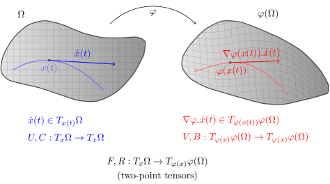
Figure 19: Various linear mappings between the tangent spaces $T_{x}\Omega$ and $T_{\varphi(x)}\varphi(\Omega)$.

The right Cauchy-Green tensor $C=F^{T}F$, in particular, is often interpreted as a Riemannian metric on $\Omega$; Epstein [61, p. 113] explains that “the right Cauchy-Green tensor is precisely the pull-back of the spatial metric to the body manifold”, cf. [127]. If $\Omega$ and $\varphi(\Omega)$ are embedded in the Euclidean space $\mathbb{R}^{n}$, this connection can immediately be seen: while the length of a curve $x\colon[0,1]\to\Omega$ is given by $\int_{0}^{1}\sqrt{\langle{\dot{x}},{\dot{x}}\rangle}\,{\mathrm{d}t}$, where $\langle\cdot,\cdot\rangle$ is the canonical inner product on $\mathbb{R}^{n}$, the length of the deformed curve $\varphi\circ x$ is given by (cf. Figure 19)

$$\int_{0}^{1}\sqrt{\langle\tfrac{\mathrm{d}}{\mathrm{d}t}(\varphi\circ x),\;\tfrac{\mathrm{d}}{\mathrm{d}t}(\varphi\circ x)\rangle}\,{\mathrm{d}t}=\int_{0}^{1}\sqrt{\langle F(x)\,{\dot{x}},\,F(x)\,{\dot{x}}\rangle}\,{\mathrm{d}t}=\int_{0}^{1}\sqrt{\langle C(x)\,{\dot{x}},\,{\dot{x}}\rangle}\,{\mathrm{d}t}\,.$$

The quadratic form $g_{x}(v,v)=\langle C(x)\,v,\,v\rangle$ at $x\in\Omega$ therefore measures the length of the deformed line element $Fv$ at $\varphi(x)\in\varphi(\Omega)$. Thus locally,

$$\operatorname{dist}_{\mathrm{Euclid,}\varphi(\Omega)}(\varphi(x),\varphi(y))=\operatorname{dist}_{\mathrm{geod,}\Omega}(x,y)\,,$$

where $\operatorname{dist}_{\mathrm{Euclid,}\varphi(\Omega)}(\varphi(x),\varphi(y))=\lVert\varphi(x)-\varphi(y)\rVert$ is the Euclidean distance between $\varphi(x),\varphi(y)\in\varphi(\Omega)$ and $\operatorname{dist}_{\mathrm{geod,}\Omega}(x,y)$ denotes the geodesic distance between $x,y\in\Omega$ with respect to the Riemannian metric $g_{x}(v,w)=\langle C(x)\,v,\,w\rangle$.

Moreover, this interpretation characterizes the Green-Lagrangian strain tensor $E_{1}=\frac{1}{2}(C-\@macros@idbb{1})$ as a measure of change in length: the difference between the squared length of a line element $v\in T_{x}\Omega$ in the reference configuration and the squared length of the deformed line element $F(x)\,v\in T_{\varphi(x)}\varphi(\Omega)$ is given by

$$\lVert F(x)\,v\rVert^{2}-\lVert v\rVert^{2}=\langle C(x)\,v,\,v\rangle-\langle v,v\rangle=\langle(C(x)-\@macros@idbb{1})\,v,\,v\rangle=2\,\langle E_{1}(x)\,v,\,v\rangle\,,$$

where $\lVert\,.\,\rVert$ denotes the Euclidean norm on $\mathbb{R}^{n}$. Note that for $F(x)=\@macros@idbb{1}+\nabla u(x)$ with the displacement gradient $\nabla u(x)$, the expression $\lVert F(x)\,v\rVert^{2}$ can be linearized to

$$\lVert F(x)\,v\rVert^{2} =\lVert(\@macros@idbb{1}+\nabla u(x))\,v\rVert^{2}=\langle(\@macros@idbb{1}+\nabla u(x))\,v,\,(\@macros@idbb{1}+\nabla u(x))\,v\rangle$$

$$=\langle v,v\rangle+2\,\langle\nabla u(x)\,v,\,v\rangle+\langle\nabla u(x)\,v,\,\nabla u(x)\,v\rangle$$

$$=\lVert v\rVert^{2}+2\,\langle\operatorname{sym}\nabla u(x)\,v,\,v\rangle+\lVert\nabla u(x)\,v\rVert^{2}$$

$$=\lVert v\rVert^{2}+2\,\langle\operatorname{sym}\nabla u(x)\,v,\,v\rangle+\mathrm{h.o.t.}\,,$$

where $\mathrm{h.o.t.}$ denotes higher order terms with respect to $\nabla u(x)$. Thus

$$\lVert F(x)\,v\rVert^{2}-\lVert v\rVert^{2}=2\,\langle\varepsilon(x)\,v,\,v\rangle+\mathrm{h.o.t.}\,,$$

where $\varepsilon=\operatorname{sym}\nabla u$ is the linear strain tensor.

A.4 Additional computations

Let $\operatorname{Cof}F=(\det F)\cdot F^{-T}$ denote the cofactor of $F\in\operatorname{GL}^{\!+}(n)$. Then the geodesic distance of $\operatorname{Cof}F$ to $\operatorname{SO}(n)$ with respect to the Riemannian metric $g$ introduced in (3.5) can be computed directly by applying Theorem 3.3:

$$\operatorname{dist}_{\mathrm{geod}}^{2}(\operatorname{Cof}F,\operatorname{SO}(n))$$

$$\hskip 19.60008pt=\mu\,\lVert\operatorname{dev}_{n}\log\sqrt{(\operatorname{Cof}F)^{T}\operatorname{Cof}F}\rVert^{2}+\frac{\kappa}{2}\,\Big{[}\operatorname{tr}\Big{(}\log\sqrt{(\operatorname{Cof}F)^{T}\operatorname{Cof}F}\Big{)}\Big{]}^{2}$$

$$\hskip 19.60008pt=\mu\,\lVert\operatorname{dev}_{n}\log\sqrt{(\det F)^{2}\cdot F^{-1}F^{-T}}\rVert^{2}+\frac{\kappa}{2}\,\Big{[}\operatorname{tr}\Big{(}\log\sqrt{(\det F)^{2}\cdot F^{-1}F^{-T}}\Big{)}\Big{]}^{2}$$

$$\hskip 19.60008pt=\mu\,\lVert\operatorname{dev}_{n}\log\sqrt{F^{-1}F^{-T}}\rVert^{2}+\frac{\kappa}{2}\,\Big{[}\operatorname{tr}\Big{(}\log\big{(}(\det F)\cdot\@macros@idbb{1}\big{)}+\log\sqrt{F^{-1}F^{-T}}\Big{)}\Big{]}^{2}$$

$$\hskip 19.60008pt=\mu\,\lVert\operatorname{dev}_{n}\log(U^{-1})\rVert^{2}+\frac{\kappa}{2}\,[\operatorname{tr}\big{(}(\ln\det F)\cdot\@macros@idbb{1}+\log(U^{-1})\big{)}]^{2}$$

$$\hskip 19.60008pt=\mu\,\lVert-\operatorname{dev}_{n}\log U\rVert^{2}+\frac{\kappa}{2}\,[n\cdot(\ln\det U)-\operatorname{tr}(\log U)]^{2}$$

$$\hskip 19.60008pt=\mu\,\lVert\operatorname{dev}_{n}\log U\rVert^{2}+\frac{\kappa\,(n-1)^{2}}{2}\,[\operatorname{tr}(\log U)]^{2}\,.$$

A.5 The principal matrix logarithm on $\operatorname{Sym^{+}}(n)$ and the matrix exponential

The following lemma states some basic computational rules for the matrix exponential $\exp\colon\mathbb{R}^{n\times n}\to\operatorname{GL}^{\!+}(n)$ and the principal matrix logarithm $\log\colon\operatorname{Sym^{+}}(n)\to\operatorname{Sym}(n)$ involving the trace operator $\operatorname{tr}$ and the deviatoric part $\operatorname{dev}_{n}X=X-\frac{\operatorname{tr}(X)}{n}\cdot\@macros@idbb{1}$ of a matrix $X\in\mathbb{R}^{n\times n}$.

Lemma A.1.

Let $X\in\mathbb{R}^{n\times n}$, $P\in\operatorname{Sym^{+}}(n)$ and $c>0$. Then

i) $$\det(\exp(X)) =e^{\operatorname{tr}(X)}\,,$$

ii) $$\exp(\operatorname{dev}_{n}X) =e^{-\frac{\operatorname{tr}(X)}{n}}\cdot\exp(X)\,,$$

iii) $$\log(c\cdot\@macros@idbb{1}) =\ln(c)\cdot\log(\@macros@idbb{1})\,,$$

iv) $$\quad\log((\det P)^{-1\!/\!\!\;n}\cdot P) =\log P-\tfrac{\ln(\det P)}{n}\cdot\@macros@idbb{1}=\operatorname{dev}_{n}\log P\,.$$

Proof.

Equality i) is well known (see e.g. [22]). Equality $iii)$ follows directly from the fact that $\exp\colon\operatorname{Sym}(n)\to\operatorname{Sym^{+}}(n)$ is bijective and that $\exp(\ln(c)\cdot\@macros@idbb{1})=e^{\ln(c)}\cdot\@macros@idbb{1}=c\cdot\@macros@idbb{1}$. Since $AB=BA$ implies $\exp(AB)=\exp(A)\exp(B)$, we find

$$\exp(\operatorname{dev}_{n}X)=\exp(X-\frac{\operatorname{tr}(X)}{n}\cdot\@macros@idbb{1})=\exp(X)\cdot\exp(-\frac{\operatorname{tr}(X)}{n}\cdot\@macros@idbb{1})=\exp(X)\cdot e^{-\frac{\operatorname{tr}(X)}{n}}\cdot\@macros@idbb{1}\,,$$

showing $ii)$. For iv), note that

$$\operatorname{tr}(\log P)=\ln(\det P)\quad\Longrightarrow\quad\log P-\tfrac{\ln(\det P)}{n}\cdot\@macros@idbb{1}=\operatorname{dev}_{n}\log P\,,$$

and

$$\exp(\operatorname{dev}_{n}\log P) =e^{-\frac{\operatorname{tr}(\log P)}{n}}\cdot\exp(\log P)$$

$$=\left(e^{\ln(\det P)}\right)^{-1\!/\!\!\;n}\cdot P=(\det P)^{-1\!/\!\!\;n}\cdot P\,.$$

according to ii). Then the injectivity of the matrix exponential on $\operatorname{Sym}(n)$ shows iv). ∎

A.6 A short biography of Heinrich Hencky

Figure 20: Hencky at MIT, age 45 [135]

Biographical information on Heinrich Hencky, as laid out in [196, 33, 95]:

• November 2, 1885: Hencky is born in Ansbach, Franken, Germany

• 1904: Hencky finishes high school in Speyer

• 1904–1908: Technische Hochschule München

• 1909: Military service with the 3rd Pioneer Battalion in München

• 1912–1913: Ph.D studies at Technische Hochschule Darmstadt

• 1910–1912: Work on the Alsatian Railways

• 1913–1915: Work for a railway company in Kharkov, Ukraine

• 1915–1918: Internment in Kharkov, Ukraine

• 1919–1920: Habilitation at Technische Hochschule Darmstadt

• 1920–1921: Technische Hochschule Dresden

• 1922–1929: Technical University of Delft

• 1930–1932: Massachusetts Institute of Technology (MIT)

• 1933–1936: Potato farming in New Hampshire

• 1936–1938: Academic work in the Soviet Union, first at Kharkov Chemical Technical Institute, then at the Mechanics Institute of Moscow University

• 1938–1950: MAN (Maschinenfabrik Augsburg-Nürnberg) in Mainz

• July 6, 1951: Hencky dies in an avalanche at age 65 during mountain climbing
  

Hencky received his diploma in civil engineering from TH München in 1908 and his Ph.D from TH Darmstadt in 1913. The title of his thesis was “Über den Spannungszustand in rechteckigen, ebenen Platten bei gleichmäßig verteilter und bei konzentrierter Belastung” (“On the stress state in rectangular flat plates under uniformly distributed and concentrated loading”). In 1915, the main results of his thesis were also published in the Zeitschrift für angewandte Mathematik und Physik [96].

After working on plasticity theory and small-deformation elasticity, he began his work on finite elastic deformations in 1928. In 1929 he introduced the logarithmic strain $\mathrm{e}_{\mathrm{log}}=\log\big{(}\frac{\text{final length}}{\text{original length}}\big{)}$ in a tensorial setting [99] and applied it to the description of the elastic behavior of vulcanized rubber [103].

Today, Hencky is mostly known for his contributions to plasticity theory: the article “Über einige statisch bestimmte Fälle des Gleichgewichts in plastischen Körpern” [98] (“On statically determined cases of equilibrium in plastic bodies”), published in 1923, is considered his most famous work [196].

References

- [1] A. H. Al-Mohy, N. J. Higham and S. D. Relton “Computing the Fréchet derivative of the matrix logarithm and estimating the condition number” In SIAM Journal on Scientific Computing 35.4 SIAM, 2013, pp. C394–C410
- [2] E. Almansi “Sulle deformazioni finite dei solidi elastici isotropi” In Rendiconti della Reale Accademia dei Lincei, Classe di scienze fisiche, matematiche e naturali 20 L’Accademia Roma, 1911
- [3] L. Anand “On H. Hencky’s approximate strain energy function for moderate deformations” In Journal of Applied Mechanics 46, 1979, pp. 78–82
- [4] L. Anand “Moderate deformations in extension-torsion of incompressible isotropic elastic materials” In Journal of the Mechanics and Physics of Solids 34, 1986, pp. 293–304
- [5] E. Andruchow, G. Larotonda, L. Recht and A. Varela “The left invariant metric in the general linear group” In Journal of Geometry and Physics 86.0, 2014, pp. 241 –257
- [6] S. S. Antman “Nonlinear problems of elasticity” 107, Applied Mathematical Sciences New York: Springer, 2005
- [7] V. Arsigny, O. Commowick, N. Ayache and X. Pennec “A fast and log-Euclidean polyaffine framework for locally linear registration” In Journal of Mathematical Imaging and Vision 33.2 Springer, 2009, pp. 222–238
- [8] V. Arsigny, P. Fillard, X. Pennec and N. Ayache “Fast and simple calculus on tensors in the log-Euclidean framework” In Medical Image Computing and Computer-Assisted Intervention–MICCAI 2005 Springer, 2005, pp. 115–122
- [9] V. Arsigny, P. Fillard, X. Pennec and N. Ayache “Geometric means in a novel vector space structure on symmetric positive-definite matrices” In SIAM Journal on Matrix Analysis and Applications 29.1 SIAM, 2007, pp. 328–347
- [10] J. M. Ball “Convexity conditions and existence theorems in nonlinear elasticity” In Archive for Rational Mechanics and Analysis 63.4 Springer, 1976, pp. 337–403
- [11] J. M. Ball “Constitutive inequalities and existence theorems in nonlinear elastostatics” In Nonlinear Analysis and Mechanics: Heriot-Watt Symposium 1, 1977, pp. 187–241 Pitman Publishing Ltd. Boston
- [12] J. M. Ball “Discontinuous equilibrium solutions and cavitation in nonlinear elasticity” In Philosophical Transactions of the Royal Society of London. Series A, Mathematical and Physical Sciences 306.1496 The Royal Society, 1982, pp. 557–611
- [13] J. M. Ball “Some open problems in elasticity” In Geometry, Mechanics, and Dynamics Springer, 2002, pp. 3–59
- [14] Daniel Balzani, Patrizio Neff, Jörg Schröder and Gerhard A Holzapfel “A polyconvex framework for soft biological tissues. Adjustment to experimental data” In International Journal of Solids and Structures 43.20 Elsevier, 2006, pp. 6052–6070 DOI: 10.1016/j.ijsolstr.2005.07.048
- [15] R. C. Batra “Linear constitutive relations in isotropic finite elasticity” In Journal of Elasticity 51.3 Springer, 1998, pp. 243–245
- [16] R. C. Batra “Comparison of results from four linear constitutive relations in isotropic finite elasticity” In International Journal of Non-Linear Mechanics 36.3 Elsevier, 2001, pp. 421–432
- [17] Z. P. Bažant “Easy-to-compute tensors with symmetric inverse approximating Hencky finite strain and its rate” In Journal of Engineering Materials and Technology 120.2 American Society of Mechanical Engineers, 1998, pp. 131–136
- [18] G. F. Becker “The Finite Elastic Stress-Strain Function” newly typeset version available at https://www.uni-due.de/imperia/md/content/mathematik/ag_neff/becker_latex_new1893.pdf In American Journal of Science 46, 1893, pp. 337–356
- [19] J.F. Bell and C. Truesdell “Mechanics of Solids: Volume 1: The Experimental Foundations of Solid Mechanics”, Handbuch der Physik Springer, 1973
- [20] E. Benvenuto “An Introduction to the History of Structural Mechanics. Part I: Statics and Resistance of Solids” Springer, 1991
- [21] J. Bernoulli “Véritable hypothèse de la résistance des solides, avec la démonstration de la courbure des corps qui font ressort” In Mémoires de l’Académie des Sciences, 1705
- [22] D. S. Bernstein “Matrix Mathematics: Theory, Facts, and Formulas (Second Edition)”, Princeton reference Princeton University Press, 2009
- [23] A. Bertram “Elasticity and Plasticity of Large Deformations” Springer, 2008
- [24] A. Bertram, T. Böhlke and M. Šilhavỳ “On the rank 1 convexity of stored energy functions of physically linear stress-strain relations” In Journal of Elasticity 86.3 Springer, 2007, pp. 235–243
- [25] R. Bhatia “Positive definite matrices” Princeton University Press, 2009
- [26] R. Bhatia and J. Holbrook “Riemannian geometry and matrix geometric means” In Linear Algebra and its Applications 413.2 Elsevier, 2006, pp. 594–618
- [27] Davide Bigoni “Nonlinear Solid Mechanics: Bifurcation Theory and Material Instability” Cambridge University Press, 2012
- [28] M. A. Biot “Non-linear theory of elasticity and the linearized case for a body under initial stress” In The London, Edinburgh, and Dublin Philosophical Magazine and Journal of Science 27.183 Taylor & Francis, 1939, pp. 468–489
- [29] Mircea Bîrsan, Patrizio Neff and Johannes Lankeit “Sum of squared logarithms - an inequality relating positive definite matrices and their matrix logarithm” In Journal of Inequalities and Applications 2013.1 Springer, 2013, pp. 1–16 DOI: 10.1186/1029-242X-2013-168
- [30] Lev Borisov, Patrizio Neff, Suvrit Sra and Christian Thiel “The sum of squared logarithms inequality in arbitrary dimensions” available at arXiv:1508.04039 In to appear in Linear Algebra and its Applications, 2015
- [31] C. Bouby, D. Fortuné, W. Pietraszkiewicz and C. Vallée “Direct determination of the rotation in the polar decomposition of the deformation gradient by maximizing a Rayleigh quotient” In Zeitschrift für Angewandte Mathematik und Mechanik 85.3 Wiley Online Library, 2005, pp. 155–162
- [32] R. Brannon “Define your strain!” available at www.mech.utah.edu/~brannon/public/strain.pdf
- [33] O. T. Bruhns “Some remarks on the history of plasticity – Heinrich Hencky, a pioneer of the early years” In The History of Theoretical, Material and Computational Mechanics - Mathematics Meets Mechanics and Engineering Springer, 2014, pp. 133–152
- [34] O. T. Bruhns “The Prandtl-Reuss equations revisited” In Zeitschrift für Angewandte Mathematik und Mechanik 94.3, 2014, pp. 187–202
- [35] O. T. Bruhns, A. Meyers and H. Xiao “On non-corotational rates of Oldroyd’s type and relevant issues in rate constitutive formulations” In Proceedings of the Royal Society of London. A. Mathematical and Physical Sciences 460.2043 The Royal Society, 2004, pp. 909–928 DOI: 10.1098/rspa.2003.1184
- [36] O. T. Bruhns, H. Xiao and A. Mayers “Constitutive inequalities for an isotropic elastic strain energy function based on Hencky’s logarithmic strain tensor” In Proceedings of the Royal Society of London. A. Mathematical and Physical Sciences 457, 2001, pp. 2207–2226
- [37] Otto T. Bruhns “The multiplicative decomposition of the deformation gradient in plasticity—origin and limitations” In From Creep Damage Mechanics to Homogenization Methods - A Liber Amicorum to celebrate the birthday of Nobutada Ohno 64 Springer International Publishing, 2015, pp. 37–66
- [38] M. M. Carroll “Must elastic materials be hyperelastic?” In Mathematics and Mechanics of Solids 14.4, 2009, pp. 369–376
- [39] M. M. Carroll and F. J. Rooney “Implications of Shield’s inverse deformation theorem for compressible finite elasticity” In Zeitschrift für angewandte Mathematik und Physik 56.6 Springer, 2005, pp. 1048–1060
- [40] A. L. Cauchy “Cours d’analyse de l’École royale polytechnique: I. Analyse algébrique” available at https://archive.org/details/coursdanalysede00caucgoog Paris: Impr. royale Debure frères, 1821
- [41] A. L. Cauchy “Sur la condensation et la dilatation des corps solides” In Exercices de Mathématiques 2 Chez de Bure frères, 1827, pp. 60–69
- [42] A. L. Cauchy “Mémoire sur les dilatations, les condensations et les rotations produits par un changement de forme dans un système de points matériels” available at http://gallica.bnf.fr/ark:/12148/bpt6k90204r/f346 In Œuvres complètes d’Augustin Cauchy XII Gauthier-Villars, 1841
- [43] I. Chao, U. Pinkall, P. Sanan and P. Schröder “A simple geometric model for elastic deformations” In ACM Transactions on Graphics 29.4, 2010, pp. 38:1–38:6 ACM
- [44] P. G. Ciarlet “Three-Dimensional Elasticity”, Studies in Mathematics and its Applications 1 Elsevier Science, 1988
- [45] J. C. Criscione “Direct tensor expression for natural strain and fast, accurate approximation” In Computers and Structures 80.25 Elsevier, 2002, pp. 1895–1905
- [46] J. C. Criscione, J. D. Humphrey, A. S. Douglas and W. C. Hunter “An invariant basis for natural strain which yields orthogonal stress response terms in isotropic hyperelasticity” In Journal of the Mechanics and Physics of Solids 48.12 Elsevier, 2000, pp. 2445–2465
- [47] A. Curnier and L. Rakotomanana “Generalized strain and stress measures: critical survey and new results” In Engineering Transactions, Polish Academy of Sciences 39.3-4, 1991, pp. 461–538
- [48] Fozi M Dannan, Patrizio Neff and Christian Thiel “On the sum of squared logarithms inequality and related inequalities” availabelt at arXiv:1411.1290 In to appear in JMI: Journal of Mathematical Inequalities, 2014
- [49] H. Darijani and R. Naghdabadi “Constitutive modeling of solids at finite deformation using a second-order stress-strain relation” In International Journal of Engineering Science 48.2, 2010, pp. 223 –236
- [50] C. De Boor “A naive proof of the representation theorem for isotropic, linear asymmetric stress-strain relations” In Journal of Elasticity 15.2 Martinus Nijhoff, The Hague/Kluwer Academic Publishers, 1985, pp. 225–227 DOI: 10.1007/BF00041995
- [51] J. Diani and P. Gilormini “Combining the logarithmic strain and the full-network model for a better understanding of the hyperelastic behavior of rubber-like materials” In Journal of the Mechanics and Physics of Solids 53.11 Elsevier, 2005, pp. 2579–2596
- [52] J.K. Dienes “On the analysis of rotation and stress rate in deforming bodies” In Acta Mechanica. 32, 1979, pp. 217–232
- [53] P. Dłużewski “Anisotropic hyperelasticity based upon general strain measures” In Journal of Elasticity 60, 2000, pp. 119–129
- [54] P. Dłużewski and P. Traczykowski “Numerical simulation of atomic positions in quantum dot by means of molecular statics.” In Archives of Mechanics 55, 2003, pp. 501–514
- [55] A. Dolcetti and D. Pertici “Some differential properties of with the trace metric” In Rivista di Matematica della Università di Parma 6, 2015, pp. 267–286
- [56] G. Dolzmann “Regularity of minimizers in nonlinear elasticity – the case of a one-well problem in nonlinear elasticity” In Technische Mechanik 32, 2012, pp. 189–194
- [57] G. Dolzmann, J. Kristensen and K. Zhang “BMO and uniform estimates for multi-well problems” In Manuscripta Mathematica 140.1-2 Springer, 2013, pp. 83–114
- [58] T. C. Doyle and J. L. Ericksen “Nonlinear elasticity” In Advances in Applied Mechanics 4 Elsevier, 1956, pp. 53–115
- [59] B. Eidel, P. Neff and R. J. Martin “Tractatus mathematicus-mechanicus modis deformationibus sub aspecto geometriae differentialis” In in preparation, 2016
- [60] B. Eidel and A. Stukowski “A variational formulation of the quasicontinuum method based on energy sampling in clusters” In Journal of the Mechanics and Physics of Solids 57.1 Elsevier, 2009, pp. 87–108
- [61] M. Epstein “The Geometrical Language of Continuum Mechanics” Cambridge University Press, 2010
- [62] L. Euler “Methodus inveniendi lineas curvas maximi minimive proprietate gaudentes (appendix, de curvis elasticis)”, 1774
- [63] S. Federico “Some Remarks on Metric and Deformation” In Mathematics and Mechanics of Solids 20, 2015, pp. 522–539
- [64] Z. Fiala “Time derivative obtained by applying the Riemannian manifold of Riemannian metrics to kinematics of continua” In Comptes Rendus Mecanique 332.2 Elsevier, 2004, pp. 97–102
- [65] Z. Fiala “Geometrical setting of solid mechanics” In Annals of Physics 326.8 Elsevier, 2011, pp. 1983–1997
- [66] Z. Fiala “Evolution equation of Lie-type for finite deformations, time-discrete integration, and incremental methods” In Acta Mechanica 226.1 Springer, 2014, pp. 17–35
- [67] Z. Fiala “Discussion of ”On the interpretation of the logarithmic strain tensor in an arbitrary system of representation“ by M. Latorre and F.J. Montáns” In International Journal of Solids and Structures 56–57.0, 2015, pp. 290 –291
- [68] Z. Fiala “Geometry of finite deformations and time-incremental analysis” In International Journal of Non-Linear Mechanics 81, 2016, pp. 230–244
- [69] J. Finger “Das Potential der inneren Kräfte und die Beziehungen zwischen den Deformationen und den Spannungen in elastisch isotropen Körpern bei Berücksichtigung von Gliedern, die bezüglich der Deformationselemente von dritter, beziehungsweise zweiter Ordnung sind” In Sitzungsberichte der Akademie der Wissenschaften in Wien 44 Verlag der Österreichischen Akademie der Wissenschaften, 1894
- [70] Andreas Fischle and Patrizio Neff “The geometrically nonlinear Cosserat micropolar shear-stretch energy. Part I: A general parameter reduction formula and energy-minimizing microrotations in 2D” available at arXiv:1507.05480 In to appear in Zeitschrift für Angewandte Mathematik und Mechanik, 2015
- [71] Andreas Fischle and Patrizio Neff “The geometrically nonlinear Cosserat micropolar shear-stretch energy. Part II: Non-classical energy-minimizing microrotations in 3D and their computational validation” available at arXiv:1509.06236 In submitted, 2015
- [72] J. E. Fitzgerald “A tensorial Hencky measure of strain and strain rate for finite deformations” In Journal of Applied Physics 51.10 AIP Publishing, 1980, pp. 5111–5115
- [73] P. J. Flory “Thermodynamic relations for high elastic materials” In Transactions of the Faraday Society 57 The Royal Society of Chemistry, 1961, pp. 829–838
- [74] R. L. Fosdick and A. S. Wineman “On general measures of deformation” In Acta Mechanica 6.4 Springer, 1968, pp. 275–295
- [75] A. D. Freed “Natural strain” In Journal of Engineering Materials and Technology 117.4 American Society of Mechanical Engineers, 1995, pp. 379–385
- [76] A. D. Freed “Hencky strain and logarithmic rates in Lagrangian analysis” In International Journal of Engineering Science 81 Elsevier, 2014, pp. 135–145
- [77] Alan D. Freed “Soft Solids - A Primer to the Theoretical Mechanics of Materials” Birkhäuser Basel, 2014
- [78] G. Friesecke, R. D. James and S. Müller “A theorem on geometric rigidity and the derivation of nonlinear plate theory from three-dimensional elasticity” In Communications on Pure and Applied Mathematics 55.11 Wiley Subscription Services, Inc., A Wiley Company, 2002, pp. 1461–1506
- [79] H. Gercek “Poisson’s ratio values for rocks” In International Journal of Rock Mechanics and Mining Sciences 44.1 Elsevier, 2007, pp. 1–13
- [80] Ionel-Dumitrel Ghiba, Patrizio Neff and Miroslav Šilhavỳ “The exponentiated Hencky-logarithmic strain energy. Improvement of planar polyconvexity” In International Journal of Non-Linear Mechanics 71 Elsevier, 2015, pp. 48–51 DOI: 10.1016/j.ijnonlinmec.2015.01.009
- [81] G. Green “On the propagation of light in crystallized media” In Transactions of the Cambridge Philosophical Society 7, 1841, pp. 121
- [82] G. Grioli “Una proprieta di minimo nella cinematica delle deformazioni finite.” In Bollettino dell’Unione Matematica Italiana 2, 1940, pp. 252–255
- [83] G. Grioli “Mathematical Theory of Elastic Equilibrium (recent results)” 7, Ergebnisse der angewandten Mathematik Springer, 1962
- [84] G. Grioli “On the thermodynamic potential for continuums with reversible transformations - some possible types” In Meccanica 1.1-2 Springer, 1966, pp. 15–20
- [85] P. Grohs, H. Hardering and O. Sander “Optimal a priori discretization error bounds for geodesic finite elements” In Foundations of Computational Mathematics Springer, 2013, pp. 1–55
- [86] M. E. Gurtin and K. Spear “On the relationship between the logarithmic strain rate and the stretching tensor” In International Journal of Solids and Structures 19.5 Elsevier, 1983, pp. 437–444
- [87] K. Hackl, A. Mielke and D. Mittenhuber “Dissipation distances in multiplicative elastoplasticity” In Analysis and Simulation of Multifield Problems Springer, 2003, pp. 87–100
- [88] M. Hanin and M. Reiner “On isotropic tensor-functions and the measure of deformation” In Zeitschrift für angewandte Mathematik und Physik 7.5 Springer, 1956, pp. 377–393
- [89] E. Hartig “Der Elastizitätsmodul des geraden Stabes als Funktion der spezifischen Beanspruchung” available at www.uni-due.de/imperia/md/content/mathematik/ag_neff/hartig_elastizitaetsmodul.pdf In Der Civilingenieur 39, 1893, pp. 113–138
- [90] P. Haupt “Continuum Mechanics and Theory of Materials.” Heidelberg: Springer, 2000
- [91] P. Haupt and C. Tsakmakis “On the application of dual variables in continuum mechanics.” In Continuum Mechanics and Thermodynamics 1, 1989, pp. 165–196
- [92] D. L. Henann and L. Anand “A large deformation theory for rate-dependent elastic–plastic materials with combined isotropic and kinematic hardening” In International Journal of Plasticity 25.10 Elsevier, 2009, pp. 1833–1878
- [93] D. L. Henann and L. Anand “Fracture of metallic glasses at notches: effects of notch-root radius and the ratio of the elastic shear modulus to the bulk modulus on toughness” In Acta Materialia 57.20 Elsevier, 2009, pp. 6057–6074
- [94] D. L. Henann and L. Anand “A large strain isotropic elasticity model based on molecular dynamics simulations of a metallic glass” In Journal of Elasticity 104.1-2 Springer, 2011, pp. 281–302
- [95] G. R. Hencky “Obituary of Gerhard R. Hencky, son of Heinrich Hencky” Published in San Francisco Chronicle. available at http://www.legacy.com/obituaries/sfgate/obituary.aspx?pid=169558738, 2014
- [96] H. Hencky “Über den Spannungszustand in kreisrunden Platten mit verschwindender Biegungssteifigkeit” In Zeitschrift für Mathematik und Physik 63, 1915, pp. 311–317
- [97] H. Hencky “Über die Beziehungen der Philosophie des ,,Als Ob” zur mathematischen Naturbeschreibung” available at https://www.uni-due.de/imperia/md/content/mathematik/ag_neff/hencky_als_ob.pdf In Annalen der Philosophie 3, 1923, pp. 236–245
- [98] H. Hencky “Über einige statisch bestimmte Fälle des Gleichgewichts in plastischen Körpern” In Zeitschrift für Angewandte Mathematik und Mechanik 3.4, 1923, pp. 241–251
- [99] H. Hencky “Über die Form des Elastizitätsgesetzes bei ideal elastischen Stoffen” available at www.uni-due.de/imperia/md/content/mathematik/ag_neff/hencky1928.pdf In Zeitschrift für technische Physik 9, 1928, pp. 215–220
- [100] H. Hencky “Das Superpositionsgesetz eines endlich deformierten relaxationsfähigen elastischen Kontinuums und seine Bedeutung für eine exakte Ableitung der Gleichungen für die zähe Flüssigkeit in der Eulerschen Form” available at https://www.uni-due.de/imperia/md/content/mathematik/ag_neff/hencky_superposition1929.pdf In Annalen der Physik 394.6, 1929, pp. 617–630
- [101] H. Hencky “Welche Umstände bedingen die Verfestigung bei der bildsamen Verformung von festen isotropen Körpern?” available at www.uni-due.de/imperia/md/content/mathematik/ag_neff/hencky1929.pdf In Zeitschrift für Physik 55, 1929, pp. 145–155
- [102] H. Hencky “The law of elasticity for isotropic and quasi-isotropic substances by finite deformations” available at https://www.uni-due.de/imperia/md/content/mathematik/ag_neff/henckyjrheology31.pdf In Journal of Rheology 2.2, 1931, pp. 169–176
- [103] H. Hencky “The elastic behavior of vulcanized rubber” available at https://www.uni-due.de/imperia/md/content/mathematik/ag_neff/hencky_vulcanized_rubber.pdf In Rubber Chemistry and Technology 6.2, 1933, pp. 217–224
- [104] N. J. Higham “Matrix Nearness Problems and Applications” University of Manchester. Department of Mathematics, 1988
- [105] N. J. Higham “Functions of Matrices: Theory and Computation” Philadelphia, PA, USA: Society for IndustrialApplied Mathematics, 2008
- [106] R. Hill “On constitutive inequalities for simple materials - I” In Journal of the Mechanics and Physics of Solids 11, 1968, pp. 229–242
- [107] R. Hill “Constitutive inequalities for isotropic elastic solids under finite strain” In Proceedings of the Royal Society of London. A. Mathematical and Physical Sciences 314, 1970, pp. 457–472
- [108] R. Hill “Aspects of invariance in solid mechanics” In Advances in Applied Mechanics 18, 1978, pp. 1–75
- [109] A. Hoger “The stress conjugate to logarithmic strain.” In International Journal of Solids and Structures 23, 1987, pp. 1645–1656
- [110] R. Hooke “Lectures de potentia restitutiva, or of Spring, Explaining the Power of Springy Bodies (1678)” In Early Science in Oxford, Volume VIII: The Cutler Lectures of Robert Hooke Oxford University Press, 1931
- [111] H. Hopf and W. Rinow “Über den Begriff der vollständigen differentialgeometrischen Fläche” In Commentarii Mathematici Helvetici 3.1 Springer, 1931, pp. 209–225
- [112] T. Hughes and J. E. Marsden “Some applications of geometry in continuum mechanics” In Reports on Mathematical Physics 12, 1977, pp. 35–44
- [113] J. W. Hutchinson and K. W Neale “Finite Strain -Deformation Theory” In Proceedings of the IUTAM Symposium on Finite Elasticity, 1982, pp. 237–247
- [114] A. Imbert “Recherches théoriques et expérimentales sur l’élasticité du caoutchouc” available at www.uni-due.de/imperia/md/content/mathematik/ag_neff/imbert_rubber.pdf Lyon: Goyard, 1880
- [115] D. F. Jones and L. R. G. Treloar “The properties of rubber in pure homogeneous strain” In Journal of Physics D: Applied Physics 8.11 IOP Publishing, 1975, pp. 1285
- [116] J. Jost “Riemannian Geometry and Geometric Analysis (2nd ed.)” Springer, 1998
- [117] G. R. Kirchhoff “Über die Gleichungen des Gleichgewichtes eines elastischen Körpers bei nicht unendlich kleinen Verschiebungen seiner Theile” In Sitzungsberichte der Mathematisch-Naturwissenschaftlichen Classe der Kaiserlichen Akademie der Wissenschaften in Wien IX Wien: Verlag der Österreichischen Akademie der Wissenschaften, 1852
- [118] Johannes Lankeit, Patrizio Neff and Yuji Nakatsukasa “The minimization of matrix logarithms: On a fundamental property of the unitary polar factor” In Linear Algebra and its Applications 449 Elsevier, 2014, pp. 28–42 DOI: 10.1016/j.laa.2014.02.012
- [119] M. Latorre and F. J. Montáns “On the interpretation of the logarithmic strain tensor in an arbitrary system of representation” In International Journal of Solids and Structures 51.7 Elsevier, 2014, pp. 1507–1515
- [120] M. Latorre and F. J. Montáns “Response to Fiala’s comments on ’On the interpretation of the logarithmic strain tensor in an arbitrary system of representation”’ In International Journal of Solids and Structures, 2015, pp. 292
- [121] H. Le Dret and A. Raoult “The quasiconvex envelope of the Saint Venant–Kirchhoff stored energy function” In Proceedings of the Royal Society of Edinburgh: Section A Mathematics 125.06 Cambridge University Press, 1995, pp. 1179–1192
- [122] T. Lehmann “Anisotrope plastische Formänderungen” In Romanian Journal of Technical Sciences. Applied Mechanics 17, 1972, pp. 1077–1086
- [123] G. W. Leibniz “Letter to Jacob Bernoulli, September 24, 1690” In Leibniz: Sämtliche Schriften und Briefe, Reihe III: Mathematischer, naturwissenschaftlicher und technischer Briefwechsel 4 Berlin: Akademie Verlag, 1995
- [124] P. Ludwik “Elemente der technologischen Mechanik” available at https://www.uni-due.de/~hm0014/ag_neff/ludwik.pdf Berlin: J. Springer, 1909
- [125] A. I. Lurie “Nonlinear Theory of Elasticity” Elsevier, 2012
- [126] C.S. Man “Hartig’s law and linear elasticity with initial stress.” In Inverse Problems. 14, 1998, pp. 313–319.
- [127] J. E. Marsden and T. Hughes “Mathematical Foundations of Elasticity” Courier Dover Publications, 1994
- [128] R. J. Martin and P. Neff “The -geodesic distance on ” In in preparation, 2016
- [129] Robert J. Martin and Patrizio Neff “Minimal geodesics on GL(n) for left-invariant, right-O(n)-invariant Riemannian metrics” available at arXiv:1409.7849 In to appear in The Journal of Geometric Mechanics, 2014
- [130] Robert J. Martin and Patrizio Neff “Some remarks on the monotonicity of primary matrix functions on the set of symmetric matrices” In Archive of Applied Mechanics 85.12 Springer, 2015, pp. 1761–1778 DOI: 10.1007/s00419-015-1017-4
- [131] L. C. Martins and P. Podio-Guidugli “A variational approach to the polar decomposition theorem” In Rendiconti delle sedute dell’Accademia nazionale dei Lincei 66.6, 1979, pp. 487–493
- [132] L. C. Martins and P. Podio-Guidugli “An elementary proof of the polar decomposition theorem” In The American Mathematical Monthly 87, 1980, pp. 288–290
- [133] G. Merrill “Biographical memoir George Ferdinand Becker” In Memoirs National Academy of Science, XXI, 1927
- [134] A. Mielke “Finite elastoplasticity, Lie groups and geodesics on ” In Geometry, Mechanics, and Dynamics - Volume in Honor of the 60th Birthday of J.E. Marsden Springer New York, 2002, pp. 61–90
- [135] P. W. Mitchell “Hencky’s remarkable equation” In Australian Geomechanics 44.4, 2009, pp. 41
- [136] M. Moakher “Means and averaging in the group of rotations” In SIAM Journal on Matrix Analysis and Applications 24.1 Philadelphia, PA, USA: Society for IndustrialApplied Mathematics, 2002, pp. 1–16
- [137] M. Moakher “A differential geometric approach to the geometric mean of symmetric positive-definite matrices” In SIAM Journal on Matrix Analysis and Applications 26.3 SIAM, 2005, pp. 735–747
- [138] M. Moakher and A. N. Norris “The closest elastic tensor of arbitrary symmetry to an elasticity tensor of lower symmetry” In Journal of Elasticity 85.3 Springer, 2006, pp. 215–263
- [139] M. Moakher and M. Zéraï “The Riemannian geometry of the space of positive-definite matrices and its application to the regularization of positive-definite matrix-valued data” In Journal of Mathematical Imaging and Vision 40.2, 2010, pp. 171–187
- [140] Giuseppe Montella, Sanjay Govindjee and Patrizio Neff “The exponentiated Hencky strain energy in modelling tire derived material for moderately large deformations” available at arXiv:1509.06541 In to appear in Journal of Engineering Materials and Technology, Transaction of the ASME, 2015
- [141] A. E. Moyer “Robert Hooke’s ambiguous presentation of “Hooke’s law”” In Isis 68.2 The University of Chicago Press on behalf of The History of Science Society, 1977, pp. 266–275
- [142] J. G. Murphy “Linear isotropic relations in finite hyperelasticity: some general results” In Journal of Elasticity 86.2 Springer, 2007, pp. 139–154
- [143] S. Müller and S. J. Spector “An existence theory for nonlinear elasticity that allows for cavitation” In Archive for Rational Mechanics and Analysis 131.1 Springer-Verlag, 1995, pp. 1–66
- [144] P. Neff “Mathematische Analyse multiplikativer Viskoplastizität. Ph.D. Thesis, Technische Universität Darmstadt.” available at http://www.uni-due.de/~hm0014/Download_files/neffdiss.ps Aachen: Shaker Verlag, 2000
- [145] P. Neff “A new support for using Hencky’s strain measure in finite elasticity - Seminar at the International Research Center for Mathematics and Mechanics of Complex Systems, Cisterna di Latina, Italy. Invitation by F. dell’Isola” Accessed: 2015-03-05, http://memocs.univaq.it/?p=4184, 2013
- [146] P. Neff, B. Eidel and R. J. Martin “The axiomatic deduction of the quadratic Hencky strain energy by Heinrich Hencky (a new translation of Hencky’s original German articles)” In arXiv:1402.4027, 2014
- [147] P. Neff, B. Eidel, F. Osterbrink and R. Martin “A Riemannian approach to strain measures in nonlinear elasticity” In Comptes Rendus Mécanique 342.4, 2014, pp. 254–257
- [148] P. Neff, B. Eidel, F. Osterbrink and R. J. Martin “The Hencky strain energy measures the geodesic distance of the deformation gradient to in the canonical left-invariant Riemannian metric on ” In Proceedings in Applied Mathematics and Mechanics 13.1, 2013, pp. 369–370
- [149] P. Neff, A. Fischle and I. Münch “Symmetric Cauchy-stresses do not imply symmetric Biot-strains in weak formulations of isotropic hyperelasticity with rotational degrees of freedom.” In Acta Mechanica 197, 2008, pp. 19–30
- [150] P. Neff, J. Lankeit and A. Madeo “On Grioli’s minimum property and its relation to Cauchy’s polar decomposition” In International Journal of Engineering Science 80.0, 2014, pp. 209–217
- [151] P. Neff and I. Münch “Curl bounds Grad on .” In ESAIM: Control, Optimisation and Calculus of Variations 14.1, 2008, pp. 148–159
- [152] P. Neff, I. Münch and R. J. Martin “Rediscovering G. F. Becker’s early axiomatic deduction of a multiaxial nonlinear stress-strain relation based on logarithmic strain” available at arXiv:1403.4675 In to appear in Mathematics and Mechanics of Solids, doi: 10.1177/1081286514542296, 2014 DOI: 10.1177/1081286514542296
- [153] Patrizio Neff and Ionel-Dumitrel Ghiba “The exponentiated Hencky-logarithmic strain energy. Part III: Coupling with idealized isotropic finite strain plasticity” In Continuum Mechanics and Thermodynamics 28.1 Springer, 2016, pp. 477–487 DOI: 10.1007/s00161-015-0449-y
- [154] Patrizio Neff, Ionel-Dumitrel Ghiba and Johannes Lankeit “The exponentiated Hencky-logarithmic strain energy. Part I: Constitutive issues and rank-one convexity” In Journal of Elasticity 121.2 Springer, 2015, pp. 143–234 DOI: 10.1007/s10659-015-9524-7
- [155] Patrizio Neff, Johannes Lankeit, Ionel-Dumitrel Ghiba, Robert J. Martin and David J. Steigmann “The exponentiated Hencky-logarithmic strain energy. Part II: coercivity, planar polyconvexity and existence of minimizers” In Zeitschrift für angewandte Mathematik und Physik 66.4 Springer, 2015, pp. 1671–1693 DOI: 10.1007/s00033-015-0495-0
- [156] Patrizio Neff, Yuji Nakatsukasa and Andreas Fischle “A logarithmic minimization property of the unitary polar factor in the spectral and Frobenius norms” In SIAM Journal on Matrix Analysis and Applications 35.3 SIAM, 2014, pp. 1132–1154 DOI: 10.1137/130909949
- [157] A. N. Norris “The isotropic material closest to a given anisotropic material” In Journal of Mechanics of Materials and Structures 1.2, 2006, pp. 223–238
- [158] A. N. Norris “Eulerian conjugate stress and strain” In Journal of Mechanics of Materials and Structures 3.2, 2008, pp. 243–260
- [159] A. N. Norris “Higher derivatives and the inverse derivative of a tensor-valued function of a tensor” In Quarterly of Applied Mathematics 66, 2008, pp. 725–741
- [160] R. W. Ogden “Compressible isotropic elastic solids under finite strain - constitutive inequalities” In The Quarterly Journal of Mechanics and Applied Mathematics 23.4, 1970, pp. 457–468
- [161] R. W. Ogden “On stress rates in solid mechanics with application to elasticity theory” In Mathematical Proceedings of the Cambridge Philosophical Society 75, 1974, pp. 303–319
- [162] R. W. Ogden “Non-Linear Elastic Deformations.”, Mathematics and its Applications Chichester: Ellis Horwood, 1983
- [163] A. Ohara, N. Suda and S. Amari “Dualistic differential geometry of positive definite matrices and its applications to related problems” In Linear Algebra and its Applications 247, 1996, pp. 31–53
- [164] W. A. Oldfather, C. A. Ellis and D. M. Brown “Leonhard Euler’s elastic curves” In Isis 20.1 JSTOR, 1933, pp. 72–160
- [165] M. Ortiz, R. A. Radovitzky and E. A. Repetto “The computation of the exponential and logarithmic mappings and their first and second linearizations” In International Journal for Numerical Methods in Engineering 52.12, 2001, pp. 1431–1441
- [166] X. Pennec “Emerging Trends in Visual Computing” Berlin, Heidelberg: Springer-Verlag, 2009, pp. 347–386
- [167] X. Pennec, P. Fillard and N. Ayache “A Riemannian framework for tensor computing” In International Journal of Computer Vision 66.1, 2006, pp. 41–66
- [168] J. P. Poirier and A. Tarantola “A logarithmic equation of state” In Physics of the Earth and Planetary Interiors 109.1 Elsevier, 1998, pp. 1–8
- [169] S. D. Poisson “Mémoire sur l’équilibre et mouvement des corps élastiques” Paris: L’Académie des sciences, 1829
- [170] Waldemar Pompe and Patrizio Neff “On the generalised sum of squared logarithms inequality” In Journal of Inequalities and Applications 2015.1 Springer, 2015, pp. 1–17 DOI: 10.1186/s13660-015-0623-6
- [171] L. Prandtl “Elastisch bestimmte und elastisch unbestimmte Systeme” In Beiträge zur Technischen Mechanik und Technischen Physik Springer Berlin Heidelberg, 1924, pp. 52–61 DOI: 10.1007/978-3-642-51983-3˙8
- [172] W. D. Reinhardt and R. N. Dubey “Eulerian strain-rate as a rate of logarithmic strain” In Mechanics Research Communications 22.2 Elsevier, 1995, pp. 165–170
- [173] W. D. Reinhardt and R. N. Dubey “Application of objective rates in mechanical modeling of solids” In Journal of applied mechanics 63.3 American Society of Mechanical Engineers, 1996, pp. 692–698
- [174] J. G. Rešetnjak “Liouville’s conformal mapping theorem under minimal regularity hypotheses” In Sibirskii Matematicheskii Zhurnal 8, 1967, pp. 835–840
- [175] H. Richter “Das isotrope Elastizitätsgesetz” available at https://www.uni-due.de/imperia/md/content/mathematik/ag_neff/richter_isotrop_log.pdf In Zeitschrift für Angewandte Mathematik und Mechanik 28.7/8, 1948, pp. 205–209
- [176] H. Richter “Verzerrungstensor, Verzerrungsdeviator und Spannungstensor bei endlichen Formänderungen” available at https://www.uni-due.de/imperia/md/content/mathematik/ag_neff/richter_deviator_log.pdf In Zeitschrift für Angewandte Mathematik und Mechanik 29.3, 1949, pp. 65–75
- [177] H. Richter “Zum Logarithmus einer Matrix” available at https://www.uni-due.de/imperia/md/content/mathematik/ag_neff/richter_log.pdf In Archiv der Mathematik 2.5 Birkhäuser-Verlag, 1949, pp. 360–363 DOI: 10.1007/BF02036865
- [178] H. Richter “Zur Elastizitätstheorie endlicher Verformungen” In Mathematische Nachrichten 8.1, 1952, pp. 65–73
- [179] Ronald S. Rivlin “On the definition of strain” In Some recent developments in rheology : based on the 1949 Bristol Conference of the British Rheologist’s Club London: United Trade Press, 1950, pp. 125–129
- [180] P. Rougée “A new Lagrangian intrinsic approach to large deformations in continuous media” In European Journal of Mechanics - A/Solids 10.1 Elsevier, 1991, pp. 15–39
- [181] P. Rougée “The intrinsic Lagrangian metric and stress variables” In Finite Inelastic Deformations - Theory and Applications, International Union of Theoretical and Applied Mechanics Springer, 1992, pp. 217–226
- [182] P. Rougée “Mécanique des Grandes Transformations” Springer, 1997
- [183] P. Rougée “An intrinsic Lagrangian statement of constitutive laws in large strain” In Computers and Structures 84.17 Elsevier, 2006, pp. 1125–1133
- [184] O. Sander “Geodesic finite elements of higher order” preprint available at http://www.igpm.rwth-aachen.de/Download/reports/pdf/IGPM356_k.pdf In to appear in IMA Journal of Numerical Analysis, 2015
- [185] C. Sansour “On the dual variable of the logarithmic strain tensor, the dual variable of the Cauchy stress tensor, and related issues.” In International Journal of Solids and Structures 38, 2001, pp. 9221–9232
- [186] C. Sansour and H. Bednarczyk “A study on rate-type constitutive equations and the existence of a free energy function” In Acta mechanica 100.3-4 Springer, 1993, pp. 205–221
- [187] J Schröder, P Neff and V Ebbing “Anisotropic polyconvex energies on the basis of crystallographic motivated structural tensors” In Journal of the Mechanics and Physics of Solids 56.12 Elsevier, 2008, pp. 3486–3506 DOI: 10.1016/j.jmps.2008.08.008
- [188] Jörg Schröder, Patrizio Neff and Daniel Balzani “A variational approach for materially stable anisotropic hyperelasticity” In International journal of solids and structures 42.15 Elsevier, 2005, pp. 4352–4371 DOI: 10.1016/j.ijsolstr.2004.11.021
- [189] T. Sendova and J. R. Walton “On strong ellipticity for isotropic hyperelastic materials based upon logarithmic strain” In International Journal of Non-Linear Mechanics 40.2 Elsevier, 2005, pp. 195–212
- [190] B. R. Seth “Generalized strain measure with applications to physical problems”, 1961
- [191] R. T. Shield “Inverse deformation results in finite elasticity” In Zeitschrift für angewandte Mathematik und Physik 18.4 Springer, 1967, pp. 490–500
- [192] F. Sidoroff “Sur les restrictions à imposer à l’énergie de déformation d’un matériau hyperélastique” In Comptes Rendus de l’Académie des Sciences 279, 1974, pp. 379–382
- [193] M. Šilhavỳ “The Mechanics and Thermomechanics of Continuous Media”, Texts and Monographs in Physics Springer, 1997
- [194] M. Šilhavỳ “Rank 1 convex hulls of isotropic functions in dimension 2 by 2” In Mathematica Bohemica 126.2 Institute of Mathematics, Academy of Sciences of the Czech Republic, 2001, pp. 521–529
- [195] E. B. Tadmor and R. E. Miller “Modeling Materials: Continuum, Atomistic and Multiscale Techniques” Cambridge University Press, 2011
- [196] R. I. Tanner and E. Tanner “Heinrich Hencky: a rheological pioneer” In Rheologica Acta 42.1-2 Springer, 2003, pp. 93–101
- [197] A. Tarantola “Elements for Physics: Quantities, Qualities, and Intrinsic Theories.” Heidelberg: Springer, 2006
- [198] A. Tarantola “Stress and strain in symmetric and asymmetric elasticity” In available at arXiv:0907.1833, 2009
- [199] C. Truesdell “Mechanical foundations of elasticity and fluid dynamics” In Journal of Rational Mechanics and Analysis 1, 1952, pp. 125–300
- [200] C. Truesdell “Hypo-elasticity” In Journal of Rational Mechanics and Analysis 4.1, 1955, pp. 83–131
- [201] C. Truesdell “The simplest rate theory of pure elasticity” In Communications on Pure and Applied Mathematics 8.1 Wiley Subscription Services, Inc., A Wiley Company, 1955, pp. 123–132 DOI: 10.1002/cpa.3160080109
- [202] C. Truesdell “Das ungelöste Hauptproblem der endlichen Elastizitätstheorie” In Zeitschrift für Angewandte Mathematik und Mechanik 36.3-4 WILEY-VCH Verlag, 1956, pp. 97–103 DOI: 10.1002/zamm.19560360304
- [203] C. Truesdell and W. Noll “The Non-Linear Field Theories of Mechanics” In Handbuch der Physik III/3 Heidelberg: Springer, 1965
- [204] C. Truesdell and R. Toupin “The Classical Field Theories.” In Handbuch der Physik III/1 Heidelberg: Springer, 1960
- [205] C. Vallée “Lois de comportement élastique isotropes en grandes déformations” In International Journal of Engineering Science 16.7 Elsevier, 1978, pp. 451–457
- [206] C. Vallée, D. Fortuné and C. Lerintiu “On the dual variable of the Cauchy stress tensor in isotropic finite hyperelasticity” In Comptes Rendus Mecanique 336.11 Elsevier, 2008, pp. 851–855
- [207] B. Vandereycken, P.-A. Absil and S. Vandewalle “A Riemannian geometry with complete geodesics for the set of positive semidefinite matrices of fixed rank” In IMA Journal of Numerical Analysis 33, 2013, pp. 481–514
- [208] J. P. Wilber and J. C. Criscione “The Baker-Ericksen inequalities for hyperelastic models using a novel set of invariants of Hencky strain” In International Journal of Solids and Structures 42.5 Elsevier, 2005, pp. 1547–1559
- [209] H. Xiao “Hencky strain and Hencky model: extending history and ongoing tradition” In Multidiscipline Modeling in Materials and Structures 1.1, 2005, pp. 1–52
- [210] H. Xiao, O. T. Bruhns and A. Meyers “Logarithmic strain, logarithmic spin and logarithmic rate” In Acta Mechanica 124.1–4 Springer, 1997, pp. 89–105
- [211] H. Xiao, O. T. Bruhns and A. Meyers “Existence and uniqueness of the integrable-exactly hypoelastic equation and its significance to finite inelasticity” In Acta Mechanica 138.1 Springer, 1999, pp. 31–50
- [212] H Xiao, OT Bruhns and A Meyers “Hypo-elasticity model based upon the logarithmic stress rate” In Journal of Elasticity 47.1 Springer, 1997, pp. 51–68
- [213] H. Xiao and L. S. Chen “Hencky’s elasticity model and linear stress-strain relations in isotropic finite hyperelasticity” In Acta Mechanica 157.1-4 Springer, 2002, pp. 51–60
- [214] Heng Xiao and Liang-Sen Chen “Hencky’s logarithmic strain and dual stress–strain and strain–stress relations in isotropic finite hyperelasticity” In International journal of solids and structures 40.6 Elsevier, 2003, pp. 1455–1463
- [215] E. Zacur, M. Bossa and S. Olmos “Multivariate Tensor-Based Morphometry with a Right-Invariant Riemannian Distance on ” In Journal of Mathematical Imaging and Vision 50 Springer, 2014, pp. 19–31
- [216] P. A. Zhilin, H. Altenbach, E.A. Ivanova and A. Krivtsov “Material strain tensor” In Generalized Continua as Models for Materials Springer, 2013, pp. 321–331