Cooling Requirements for the Vertical Shear Instability in Protoplanetary Disks

Abstract

The vertical shear instability (VSI) offers a potential hydrodynamic mechanism for angular momentum transport in protoplanetary disks (PPDs). The VSI is driven by a weak vertical gradient in the disk’s orbital motion, but must overcome vertical buoyancy, a strongly stabilizing influence in cold disks, where heating is dominated by external irradiation. Rapid radiative cooling reduces the effective buoyancy and allows the VSI to operate. We quantify the cooling timescale $t_{c}$ needed for efficient VSI growth, through a linear analysis of the VSI with cooling in vertically global, radially local disk models. We find the VSI is most vigorous for rapid cooling with $t_{c}<\Omega_{\rm K}^{-1}h|q|/(\gamma-1)$ in terms of the Keplerian orbital frequency, $\Omega_{\rm K}$; the disk’s aspect-ratio, $h\ll 1$; the radial power-law temperature gradient, $q$; and the adiabatic index, $\gamma$. For longer $t_{c}$, the VSI is much less effective because growth slows and shifts to smaller length scales, which are more prone to viscous or turbulent decay. We apply our results to PPD models where $t_{c}$ is determined by the opacity of dust grains. We find that the VSI is most effective at intermediate radii, from $\sim 5$AU to $\sim 50$AU with a characteristic growth time of $\sim 30$ local orbital periods. Growth is suppressed by long cooling times both in the opaque inner disk and the optically thin outer disk. Reducing the dust opacity by a factor of 10 increases cooling times enough to quench the VSI at all disk radii. Thus the formation of solid protoplanets, a sink for dust grains, can impede the VSI.

1. Introduction

Understanding how disks transport mass and angular momentum underlies many problems in astrophysics, including star and planet formation (Armitage, 2011). The turbulence associated with many transport mechanisms is particularly important for dust evolution and planetesimal formation (Youdin & Lithwick, 2007; Chiang & Youdin, 2010).

Magneto-hydrodynamic (MHD) turbulence driven by the magneto-rotational instability (MRI, Balbus & Hawley, 1991) has long been the most promising transport mechanism in low mass disks with weak self-gravity. However, many parts of protoplanetary disks (PPDs) are cold, have low levels of ionization, and do not support the MRI (Blaes & Balbus, 1994; Salmeron & Wardle, 2003). Recent simulations suggest that significant portions of PPDs fail to develop MHD turbulence (e.g. Simon et al., 2013; Lesur et al., 2014; Bai, 2015; Gressel et al., 2015).

A purely hydrodynamic mechanism could circumvent difficulties with non-ideal MHD, but must overcome the strong centrifugal stability imposed by the positive radial specific angular momentum gradient in nearly Keplerian disks (Balbus et al., 1996). One possible route to hydrodynamic turbulence is the vertical shear instability (VSI, Urpin & Brandenburg, 1998; Urpin, 2003; Nelson et al., 2013, hereafter N13). The basic mechanism of the VSI in disks was first identified in the context of differentially rotating stars (Goldreich & Schubert, 1967, hereafter GS67, Fricke, 1968). The VSI arises when vertical shear, i.e. a variation in orbital motion along the rotation axis, destabilizes inertial-gravity waves, which are oscillations with rotation and buoyancy as restoring forces. Vertical shear occurs wherever the disk is baroclinic, i.e. when constant density and constant pressure surfaces are misaligned. Baroclinicity, and thus vertical shear, is practically unavoidable in astrophysical disks, except at special locations like the midplane.

To overcome centrifugal stabilization, the VSI triggers motions which are vertically elongated and radially narrow. Vertical elongation taps the free energy of the vertical shear (Umurhan et al., 2013), but is also subject to the stabilizing effects of vertical buoyancy if the disk is stably stratified. To overcome vertical buoyancy, the VSI requires a short cooling time (GS67; N13). Rapid radiative cooling, i.e. a short thermal relaxation timescale, brings a moving fluid element into thermal equilibrium with its surroundings, thereby diminishing buoyancy. An isothermal equation of state implies instantaneous thermal relaxation, and is the ideal context for studying the VSI (Urpin, 2003; N13; McNally & Pessah, 2014, hereafter MP14; Barker & Latter, 2015, hereafter BL15).

Alternatively, vertical buoyancy can be eliminated by strong internal heating, i.e. by the onset of convection, so that the disk becomes neutrally stratified in the vertical direction (; ). However, realistic PPDs should be vertically stably stratified in the outer regions, beyond $\sim 1$–5 AU, where heating is irradiation dominated (Bitsch et al., 2015). Even in the inner disk, strong vertical buoyancy is possible if accretion heating is weak or is concentrated in surface layers (Gammie, 1996; Lesniak & Desch, 2011).

Understanding the VSI in real disks therefore requires considering finite, non-zero cooling times, $t_{\rm c}$. Non-linear hydrodynamical simulations with a prescribed $t_{\rm c}$ find that VSI turbulence in stably stratified disks requires rapid cooling with $t_{\rm c}$ shorter than orbital timescales (N13). When the cooling time is short enough, the VSI can drive moderately strong transport, with Reynolds stresses of $\alpha\sim 10^{-3}$ times the mean pressure (N13). Simulations with realistic radiative transfer, in lieu of a fixed $t_{\rm c}$, find that the VSI in irradiated disks drive transport with $\alpha\sim 10^{-4}$ in a $\sim 2$ – 10AU PPD model (Stoll & Kley, 2014).

Studying the linear growth of the VSI is necessary for understanding how it can ultimately drive turbulent transport. The pioneering linear analyses of the VSI considered vertically local disturbances (Urpin & Brandenburg, 1998; Urpin, 2003). A vertical global analysis (e.g. ; ; ) is essential for understanding how vertically elongated disturbances interact with the disk’s vertical structure. Moreover a vertically global analysis allows more direct comparisons with modern numerical simulations. This work generalizes previous vertically global analyses by including a finite cooling time.

This paper is organized as follows. In §2 we explain, without derivation, our main result for the critical cooling timescale, beyond which VSI growth is suppressed. We develop our disk model in §3 and derive linearized perturbation equations in §4. Section 5 contains our main analytic results, leading to the derivation of the critical cooling time in §5.3. In §6 we analyze linear VSI growth, and numerically confirm the critical cooling time. We apply our results to PPDs in §7, with cooling times derived from dust opacities. We discuss caveats and extensions in §8. We conclude in §9 with a summary. Some technical and background developments are explained in the appendices.

2. Why must cooling be so fast?

In a stably stratified thin disk, the VSI requires a thermal timescale $t_{c}$ significantly shorter than the disk dynamical timescale,

$$t_{c}\ll\Omega_{\rm K}^{-1},$$ (1)

where $\Omega_{\rm K}$ is the Keplerian frequency (N13). This requirement — that the cooling time be much shorter than an orbital period, which in turn is much smaller than the relevant oscillation period of vertically elongated gravity waves — is quite stringent. It highlights the fact that vertical buoyancy is strongly stabilizing. Rapid radiative damping is thus required to weaken buoyancy and allow the weak vertical shear to drive instability.

To roughly quantify the required smallness of $t_{c}$, we consider a vertically isothermal disk with aspect-ratio $h$, radial temperature profile $T\propto r^{q}$ and adiabatic index $\gamma>1$ so the disk is stably stratified. For a PPD, $h\sim 0.05$, $q\sim-0.5$ and $\gamma\simeq 1.4$.

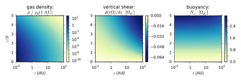
Figure 1.— The radial and vertical structure of a ‘minimum mass’ PPD model showing gas density (left, relative to the midplane density at 1 AU), vertical shear rate (middle) and buoyancy frequency (right).

For a thin disk ($h\ll 1$), the vertical shear rate varies with height, $z$, from the midplane as

$$r\frac{\partial\Omega}{\partial z}\simeq hq\Omega_{\rm K}\left(\frac{z}{2H}\right),$$ (2)

where $H=hr$ is the characteristic disk scale height.

This destabilizing shear competes with the stabilizing vertical buoyancy frequency, $N_{z}$. In a thin disk,

$$N_{z}^{2}\simeq\left(\frac{\gamma-1}{\gamma}\right)\left(\frac{z}{H}\right)^{2}\Omega_{\rm K}^{2}.$$ (3)

Fig. 1 maps the vertical shear rate and buoyancy frequency (as well as the gas density) in a fiducial PPD model, see §7.1.2 for details.

Vertical shear is generally weak compared to buoyancy, suggesting stability. In fact, without any cooling, the Solberg-Hoiland criteria confirms that vertical buoyancy is strong enough to ensure (axisymmetric) stability, see §3.4. With radiative cooling, thermal fluctuations decay which, combined with pressure equilibration, reduces the effective buoyancy.

How short must $t_{c}$ be for vertical shear to prevail? We start with the Richardson number $\mathrm{Ri}=N_{z}^{2}/(r\partial_{z}\Omega)^{2}$, a ratio of buoyant to shear energies. Though not precisely applicable to our problem, non-rotating shear flows are stable if $\mathrm{Ri}>1/4$ (Chandrasekhar, 1961, also see Youdin & Shu, 2002; Lee et al., 2010 for applications to thin dust layers in PPDs). Following Urpin (2003) and Townsend (1958), we reduce the buoyant energy by the ratio of cooling to forcing timescales, $t_{c}|r\partial_{z}\Omega|\leq 1$ (with no reduction in buoyant energy expected when this inequality fails). With this reduction, the Richardson-like criterion for shear instability becomes (Urpin, 2003)

$$t_{c}\lesssim\frac{\left|r\partial\Omega/\partial z\right|}{N_{z}^{2}}.$$ (4)

If we interpret Eq. 4 as a local criterion, then we see that the maximum cooling time which permits instability decreases with height as $1/|z|$; the stabilizing effect of vertical buoyancy increases more rapidly away from the midplane than the destabilizing effect of vertical shear. This finding is relevant to the radiative damping of so called ‘surface modes’, which we consider in §6.

We are more interested, however, in the global instability criterion for disturbances at all heights. Our key result is the cooling requirement

$$t_{c}< \frac{h|q|}{\gamma-1}\Omega_{\rm K}^{-1}$$ (5)

for VSI growth that we derive in §5.3. We can simply (but non-rigorously) obtain Eq. 5 by evaluating Eq. 4 at $|z|=\gamma H/2$.

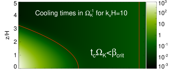
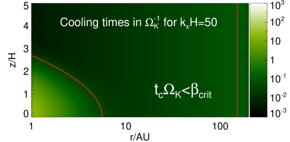
Figure 2.— Estimate of the thermal timescale $t_{c}$ in a fiducial PPD model, the Minimum Mass Solar Nebula. Here, $\beta_{\mathrm{crit}}=h|q|/(\gamma-1)$ is a maximum dimensionless cooling timescale below which the VSI is expected to operate effectively. This corresponds to the region bounded by the red lines.

We now consider whether, and where, thermal timescales in realistic PPDs are short enough to support VSI growth. Fig. 2 plots the thermal timescales in our fiducial PPD model, see §7.1.2 for details. The regions between the red lines satisfy the cooling requirement of Eq. 5. Even without a detailed analysis we can expect VSI growth between $\sim 10$ – 150AU. The inner disk is complicated by the fact that the optically thick midplane has longer cooling times. Thus the cooling criterion fails in the midplane but is satisfied above. This case requires the more detailed analysis of §7.

Fig. 2 also compares two different radial wavenumbers, $k_{x}=10/H$ and $50/H$. In the inner disk, the higher wavenumber mode cools faster, due to radiative diffusion. Thus in the inner disk, shorter wavelength VSI modes are more likely to grow. In the outer disk, the cooling time is the same for different $k_{x}$ and $z$, because optically thin cooling is independent of both lengthscale and density. Thus the outer barrier to growth, beyond $\sim 150$ AU in this model, is independent of wavelength. This example highlights the fact that optically thin cooling sets a lower limit to the cooling time; a fact that is sometimes obscured when the radiative diffusion approximation is made at the outset.

3. Governing equations and disk models

An inviscid, non-self-gravitating disk orbiting a central star of mass $M_{*}$ obeys the three-dimensional fluid equations:

$$\frac{\partial\rho}{\partial t}+\nabla\cdot{\left(\rho\bm{v}\right)}=0,$$ (6)

$$\frac{\partial\bm{v}}{\partial t}+\bm{v}\cdot\nabla\bm{v}=-\frac{1}{\rho}\nabla P-\nabla\Phi_{*},$$ (7)

$$\frac{\partial P}{\partial t}+\bm{v}\cdot\nabla P=-\gamma P\nabla\cdot\bm{v}-\Lambda,$$ (8)

where $\rho$ is the mass density, $\bm{v}$ is the velocity field (the rotation frequency being $\Omega=v_{\phi}/r$), $P$ is the pressure, $\gamma$ is the constant adiabatic index, and $\Phi_{*}=-GM_{*}(r^{2}+z^{2})^{-1/2}$ is the gravitational potential of the central star with $G$ as the gravitational constant. The cylindrical co-ordinates $(r,\phi,z)$ are centered on the star. In the energy equation (Eq. 8) the sink term $\Lambda$ includes non-adiabatic cooling and (negative) heating. The gas temperature $T$ obeys the ideal gas equation of state,

$$P=\frac{\mathcal{R}}{\mu}\rho T,$$ (9)

where $\mathcal{R}$ is the gas constant and $\mu$ is the mean molecular weight.

3.1. Thermal relaxation

We model radiative effects as thermal relaxation with a timescale $t_{c}$, i.e.,

$$\Lambda\equiv\frac{\rho\mathcal{R}}{\mu}\frac{T-T_{\mathrm{eq}}}{t_{c}},$$ (10)

where $T_{\mathrm{eq}}=T_{\mathrm{eq}}(r,z)$ is the equilibrium temperature. We define the dimensionless cooling time

$$\beta\equiv\Omega_{\rm K}t_{c}$$ (11)

relative to the Keplerian frequency, $\Omega_{\rm K}=\sqrt{GM_{*}/r^{3}}$. We use the terms ‘thermal relaxation’ and ‘cooling’ interchangeably throughout this paper.

For most of this paper we will take $\beta$ as a constant input parameter, so that we can vary the thermodynamic response of the disk from isothermal ($\beta\ll 1$) to adiabatic ($\beta\gg 1$) in a controlled manner. However, in §7 we will consider a more realistic model for $\beta$ in PPDs with a dust opacity (as in Fig.  2).

3.2. Baroclinic disk equilibria

The equilibrium disk is steady and axisymmetric with density, pressure and rotation profiles $\rho(r,z)$, $P(r,z)$ and $\Omega(r,z)$, respectively. These functions satisfy

$$0 =\frac{1}{\rho}\frac{\partial P}{\partial z}+\frac{\partial\Phi_{*}}{\partial z},$$ (12a)

$$r\Omega^{2} =\frac{1}{\rho}\frac{\partial P}{\partial r}+\frac{\partial\Phi_{*}}{\partial r}.$$ (12b)

A unique solution requires additional assumptions about disk structure. We choose

$$\rho(r,0) \equiv\rho_{0}(r)=\rho_{00}\left(\frac{r}{r_{0}}\right)^{p},$$ (13a)

$$T(r,0) \equiv T_{0}(r)=T_{00}\left(\frac{r}{r_{0}}\right)^{q},$$ (13b)

$$P(r,z) =K(r)\rho^{\Gamma}(r,z).$$ (13c)

where $r_{0}$ is a fiducial radius and $p$ and $q$ are the standard power-law indices for midplane density and temperature, respectively. Without loss of generality we take $q<0$, as is typical in PPDs. The polytropic index $\Gamma$ parametrizes the vertical stratification with $\Gamma=1$ ($\Gamma=\gamma$) describing vertically isothermal (adiabatic) disks, respectively. The ideal gas law requires $K=\rho_{0}^{1-\Gamma}\mathcal{R}T_{0}/\mu$.

We further define a modified sound speed

$$c_{s}\equiv\sqrt{\Gamma P/\rho},$$ (14)

which in general differs from the isothermal, $c_{\mathrm{iso}}=c_{s}/\sqrt{\Gamma}$, and adiabatic $c_{\mathrm{ad}}=c_{s}\sqrt{\gamma/\Gamma}$, sound speeds. We also introduce the characteristic scale-height, $H=c_{s}(r,0)/\Omega_{\rm K}$ and disk aspect-ratio

$$h(r)\equiv\frac{H}{r}\propto r^{(1+q)/2}$$ (15)

We are interested in thin disks with $h\ll 1$.

3.2.1 Density structure

The equilibrium density field follows from vertical hydrostatic equilibrium (Eq. 12a). The solution for $\Gamma\neq 1$ is

$$\left(\frac{\rho}{\rho_{0}}\right)^{\Gamma-1}=1+\frac{\left(\Gamma-1\right)}{h^{2}}\left(\frac{1}{\sqrt{1+z^{2}/r^{2}}}-1\right).$$ (16)

Note that for $\Gamma>1+h^{2}$ there is a disk surface $H_{s}$ where $\rho(r,H_{s})=0$; and $H_{s}\simeq\sqrt{2/(\Gamma-1)}H$ for $h\ll 1$.

The vertically isothermal case, $\Gamma=1$, can be calculated either as a special case or by taking the limit of Eq. 16 as $\Gamma\to 1$,

$$\frac{\rho(r,z)}{\rho_{0}(r)} =\exp{\left[\frac{1}{h^{2}}\left(\frac{1}{\sqrt{1+z^{2}/r^{2}}}-1\right)\right]},$$ (17a)

$$\simeq\exp{\left(-{z^{2}\over 2H^{2}}\right)}\quad\text{for }|z|\ll r.$$ (17b)

Eq. 17b is the approximate form of the density field in the thin-disk limit. We will primarily focus on vertically isothermal disks, the relevant case for passively irradiated PPDs (Chiang & Goldreich, 1997).

3.2.2 Rotation and vertical shear profiles

The equilibrium rotation field, $\Omega(r,z)$ follows from the density field and centrifugal balance (Eq. 12b), giving

$$\frac{\Omega^{2}(r,z)}{\Omega_{\rm K}^{2}(r)}=1+\frac{p+q}{\Gamma}h^{2}(r)+\frac{s}{\Gamma}\left(1-\frac{1}{\sqrt{1+z^{2}/r^{2}}}\right),$$ (18)

for all $\Gamma$, where $s\equiv q+p(1-\Gamma)$. We also refer to the epicyclic frequency $\kappa$ defined via

$$\kappa^{2}\equiv\frac{1}{r^{3}}\frac{\partial}{\partial r}\left(r^{4}\Omega^{2}\right)=\frac{1}{r^{3}}\frac{\partial j^{2}}{\partial r},$$ (19)

where $j$ is the specific angular momentum.

The vertical shear rate follows from Eq. 18,

$$r\frac{\partial\Omega^{2}}{\partial z}=\frac{sz}{\Gamma r}\frac{\Omega_{\rm K}^{2}}{\left(1+z^{2}/r^{2}\right)^{3/2}}.$$ (20)

For $\Gamma=1$, notice that $s/\Gamma=q$ is the only disk parameter that affects vertical shear. Vertical shear increases linearly with height near the midplane, and $|\partial_{z}\Omega^{2}|$ is maximized at $\mathrm{min}(r/\sqrt{2},H_{s})$, which is expected to limit the maximum VSI growth rate.

A more general expression for vertical shear holds for vertical polytropes (which satisfy Eq. 13c), with no assumed radial structure:

$$r\frac{\partial\Omega^{2}}{\partial z}=-\rho^{\Gamma-1}\frac{\partial\ln\rho}{\partial z}\frac{dK}{dr}=-\frac{g_{z}}{\Gamma}\frac{d\ln K}{dr},$$ (21)

where $g_{z}=\partial_{z}P/\rho$.

3.3. Entropy gradients and vertical buoyancy

The gradients of specific entropy, $S\equiv C_{P}\ln{P^{1/\gamma}/\rho}$, in our disk models are

$$\frac{\partial S}{\partial r}=C_{P}\left[\frac{s}{\gamma r}+\left(\frac{\Gamma}{\gamma}-1\right)\frac{\partial\ln{\rho}}{\partial r}\right],$$ (22a)

$$\frac{\partial S}{\partial z}=C_{P}\left(\frac{\Gamma}{\gamma}-1\right)\frac{\partial\ln{\rho}}{\partial z}={C_{P}g_{z}\over c_{s}^{2}}{\Gamma-\gamma\over\gamma},$$ (22b)

where $C_{P}$ is the heat capacity at constant pressure.

The vertical buoyancy frequency $N_{z}$ is

$$N_{z}^{2}\equiv-C_{P}^{-1}g_{z}\frac{\partial S}{\partial z}={g_{z}^{2}\over c_{s}^{2}}{\gamma-\Gamma\over\gamma}.$$ (23)

We only consider convectively stable disks with with $\Gamma<\gamma$ and $N_{z}^{2}\geq 0$.

3.4. Stability without cooling

In the absence of cooling, axisymmetric stability is ensured if both Solberg-Hoiland criteria are satisfied:

$$\kappa^{2}-\frac{1}{\rho C_{P}}\nabla P\cdot\nabla S >0,$$ (24a)

$$-\frac{\partial P}{\partial z}\left(\frac{\partial j^{2}}{\partial r}\frac{\partial S}{\partial z}-\frac{\partial j^{2}}{\partial z}\frac{\partial S}{\partial r}\right) >0$$ (24b)

(Tassoul, 1978). For rotationally-supported, thin disks the first criterion is easily satisfied. Thus, we consider the second criterion. Without loss of generality (since Eq. 24b is even in $z$), we consider $z>0$ so that $\partial_{z}P<0$. With $\partial_{r}j^{2}\simeq r^{3}\Omega_{\rm K}^{2}$ and using Eq. 21 for $\partial_{z}j^{2}$ we find that

$$\gamma-\Gamma>\frac{h^{2}}{\Gamma}\left(\frac{\rho}{\rho_{0}}\right)^{\Gamma-1}\left[s^{2}-s\left(\gamma-\Gamma\right)\frac{\partial\ln{\rho}}{\partial\ln{r}}\right]$$ (25)

implies stability. For typical model parameters, the right hand side is $O(h^{2})\lesssim 10^{-2}$. The left hand side is positive and order unity in our disk models (with $\gamma-\Gamma\geq 0.1$) implying strong stability to convection, see Eq. 23. This stable stratification is expected for irradiated disks (Chiang & Goldreich, 1997). Thus, adiabatic disturbances in a standard, irradiated disk are stable to a disk’s vertical shear, explaining why the VSI requires cooling.

4. Linear problem

This section presents the two sets of equations we use to study the linear development of the VSI. Both sets are radially local and vertically global with a finite cooling time. The first set, presented in §4.1, is more general and used for numerical calculations. The second set, in §4.2, makes additional approximations about disk structure and wave frequency. This simplified set is used to obtain analytic results.

4.1. Radially local approximation

We consider axisymmetric perturbations to the above disk equilibria. The growth of the VSI is strongest for short radial wavelengths, as compared to the disk radius (; ). We thus perform a standard two step process to obtain linearized equations in the radially local approximation (e.g., Goldreich & Schubert, 1967, who also consider vertically localized perturbations).

We first expand all fluid variables into the equilibrium value plus an Eulerian perturbation denoted by $\delta$, e.g. $\delta\rho$ for the perturbed density, and drop all non-linear perturbations. Second, we perform a Taylor expansion about a fiducial radius $r_{0}$ with the local radial coordinate $x=r-r_{0}$, keeping only the leading order terms in $x/r_{0}$. We also relabel (trivially for axisymmetric perturbations) the azimuthal direction as $y$.

Perturbations take the form of a radial plane wave with arbitrary vertical dependence, e.g.

$$\delta\rho\rightarrow\delta\rho(z)\exp{\left(\mathrm{i}k_{x}x-\mathrm{i}\upsilon t\right)},$$ (26)

where $\upsilon=\omega+\mathrm{i}\sigma$ is a (generally) complex frequency, with $\omega$ and $\sigma$ being the real frequency and growth rate, respectively, and $k_{x}$ is a real radial wavenumber. We take $k_{x}>0$ without loss of generality, assume $k_{x}r_{0}\gg 1$ and neglect curvature terms. Henceforth all unperturbed fluid variables, including gradients such as $\partial_{z}\Omega$, refer to equilibrium values at $(r_{0},z)$.

We further define the perturbation variables $W\equiv\delta P/\rho$ and $Q\equiv c_{s}^{2}\delta\rho/\rho$. With this procedure the linearized system of equations are

$$\mathrm{i}\upsilon\frac{Q}{c_{s}^{2}} =\mathrm{i}k_{x}\delta v_{x}+\frac{d\delta v_{z}}{dz}+\frac{\partial\ln{\rho}}{\partial z}\delta v_{z}+\zeta\frac{\partial\ln{\rho}}{\partial r}\delta v_{x},$$ (27a)

$$\mathrm{i}\upsilon\delta v_{x} =\mathrm{i}k_{x}W-2\Omega\delta v_{y}-\zeta\frac{1}{\rho}\frac{\partial P}{\partial r}\frac{Q}{c_{s}^{2}}$$ (27b)

$$\mathrm{i}\upsilon\delta v_{y} =r_{0}\frac{\partial\Omega}{\partial z}\delta v_{z}+\frac{\kappa^{2}}{2\Omega}\delta v_{x},$$ (27c)

$$\mathrm{i}\upsilon\delta v_{z} =\frac{dW}{dz}+\frac{\partial\ln{\rho}}{\partial z}\left(W-Q\right),$$ (27d)

$$\mathrm{i}\upsilon W =c_{s}^{2}\frac{\partial\ln{\rho}}{\partial z}\delta v_{z}+c_{s}^{2}\frac{\gamma}{\Gamma}\left(\mathrm{i}k_{x}\delta v_{x}+\frac{d\delta v_{z}}{dz}\right)$$

$$+\frac{1}{t_{c}}\left(W-\frac{Q}{\Gamma}\right)+\zeta\frac{1}{\rho}\frac{\partial P}{\partial r}\delta v_{x}.$$ (27e)

This is a set of ordinary differential equations (ODEs) in $z$. Solutions to these are presented in §6 and §7. The coefficient $\zeta=1$ is introduced simply to label terms with explicit radial gradients of the equilibrium state, which again are evaluated at $(r_{0},z)$. For clarity, hereafter we drop the subscript $0$. We will consider the effects of ignoring these radial gradients below.

4.2. Reduced equation for vertically isothermal disks

Our simplified model starts with Eqs. 27 and makes the following additional simplifications:

1. We set $\Gamma=1$, focusing on vertically isothermal disks.

2. We set $\zeta=0$, neglecting terms with an explicit dependence on the radial structure of the equilibrium disk. Vertical shear, which implicitly depends on the radial temperature gradient, is retained. This fully-radially-local approximation is also made in the ‘vertically global shearing box’ of MP14.

3. We make the low frequency approximation, assuming $|\upsilon^{2}|\ll\kappa^{2},\,\Omega^{2}$. Similar to the incompressible (GS67) or anelastic (; ) approximations, the low frequency approximation filters acoustic waves in favor of inertial-gravity waves (Lubow & Pringle, 1993).

4. We make the Keplerian approximation, setting $\Omega\rightarrow\Omega_{\rm K}$ and $\kappa\rightarrow\Omega_{\rm K}$, but retaining the vertical dependence in the crucial vertical shear term, $\partial_{z}\Omega$.

5. We consider thin disks with $h\ll 1$ and use the Gaussian approximation, Eq. 17b, for the equilibrium density field.

In terms of the dimensionless variables

$$\hat{z}=z/H,\quad\hat{k}=k_{x}H,\quad\hat{\upsilon}=\hat{\omega}+\mathrm{i}\hat{\sigma}=\upsilon/\Omega_{\rm K},$$ (28)

where $\hat{\omega}$ and $\hat{\sigma}$ are real, the above approximations lead to a single second order ODE,

$$\delta v_{z}^{\prime\prime}-zA\delta v_{z}^{\prime}+(B-C\hat{z}^{2})\delta v_{z}=0,$$ (29)

where ^′ denotes $d/d\hat{z}$ and

$$A\equiv 1+\mathrm{i}hq\hat{k},$$ (30a)

$$B\equiv\hat{\upsilon}^{2}\left(\chi+\hat{k}^{2}\right)-\left(\chi+\mathrm{i}hq\hat{k}\right),$$ (30b)

$$C\equiv\left(1-\chi\right)\left(\hat{k}^{2}-\mathrm{i}hq\hat{k}\right),$$ (30c)

where

$$\chi=\frac{1-\mathrm{i}\hat{\upsilon}\beta}{1-\mathrm{i}\hat{\upsilon}\beta\gamma}.$$ (31)

The derivation of Eq. 29 is detailed in Appendix A.

In Appendix B we discuss the limits of these approximations. In particular we point out that the fully-radially-local approximation is only valid for short cooling times, $\beta\lesssim O(1)$, which is the regime in which the VSI operates, as demonstrated below. On the other hand, for $\beta\gtrsim O(1)$, this approximation can introduce artificial instability due to the non-self-consistent neglect of global radial gradients (see §B.1).

5. Analytic results with finite cooling times

Previous analytic studies of the VSI have largely focused on isothermal perturbations, with infinitely rapid cooling, as discussed in the introduction. We further explore this $\beta=0$ limit in Appendix C both to further develop intuition for this idealized case and to establish a connection with previous works. However our main interest is the effect of finite cooling times, which we explore analytically in this section.

In §5.1 we show that even an infinitesimal increase in the cooling time, starting from $\beta=0$, slows the growth rate of the VSI. In §5.2 we derive exact solutions to the simplified VSI model developed above (Eq. 29). In §5.3 we reach our main result, the maximum cooling time above which VSI growth is suppressed.

5.1. Introducing a small but finite cooling time

We are interested in finite thermal relaxation timescales $\beta>0$, but it is instructive to first ask the more analytically tractable question: how do the eigenfrequencies and eigenfunctions change when we change $\beta$ from zero to a small but finite value? For sufficiently small $\beta$ we expect the solution to only differ slightly from a case with $\beta\equiv 0$. We thus perturb a solution for $\beta=0$ to see the effect of finite cooling.

For definiteness, let us consider the simple solution

$$\beta\equiv 0,\quad\delta v_{z}=1,\quad\hat{\upsilon}^{2}=\frac{1+\mathrm{i}hq\hat{k}}{1+\hat{k}^{2}},$$ (32)

which solves Eq. 29 since $\delta v_{z}=$constant and $\chi=1$ so that $B=C=0$. This is the lowest order VSI mode, the ‘fundamental corrugation mode’, where the vertical velocity is constant throughout the disk column. Hereafter we shall simply call it the fundamental mode.

The fundamental mode has been observed to dominate numerical simulations (Stoll & Kley, 2014, N13), and are the ones we find to typically dominate in numerical calculations with increasing $\beta$ (§6.2) for moderate values of $\hat{k}$, as well as in PPDs with a realistic estimate for thermal timescales (§7). We will see later that consideration of low order modes in fact provides a useful way to characterize the effect of increasing the thermal timescale on the VSI.

We linearize Eq. 29 about the above solution for $\beta\equiv 0$ and write

$$\beta\to 0+\delta\beta,\,\delta v_{z}\to\delta v_{z}+\delta v_{z1},\,\hat{\upsilon}\to\hat{\upsilon}+\delta\hat{\upsilon},$$ (33)

which implies

$$\chi\to 1+\delta\chi=1+\mathrm{i}\hat{\upsilon}\left(\gamma-1\right)\delta\beta,$$ (34)

with $\delta v_{z}$ and $\hat{\upsilon}$ given by Eq. 32. We may then seek

$$\delta v_{z1}=a\hat{z}^{2}+b,$$ (35)

where $a$, $b$ are constants.

We insert Eq. 33 into Eq. 29, keeping only first order terms, and solve for $\delta\hat{\upsilon}$ using the above expressions for $\delta\chi$ and $\hat{\upsilon}$. We find imaginary part of $\delta\hat{\upsilon}$ is

$$\delta\hat{\sigma}=-\frac{\left(\gamma-1\right)\hat{k}^{2}\left(\hat{k}^{2}-2h^{2}q^{2}\hat{k}^{2}-h^{2}q^{2}\right)}{2\left(1+h^{2}q^{2}\hat{k}^{2}\right)\left(1+\hat{k}^{2}\right)^{2}}\delta\beta.$$ (36)

Since $h\ll 1$, introducing finite cooling $\delta\beta>0$ implies $\delta\hat{\sigma}<0$, i.e. stabilization, since $\gamma>1$.

A finite cooling time allow buoyancy forces to stabilize vertical motions in sub-adiabatically stratified disks. The $\hat{z}^{2}$ dependence in $\delta v_{z1}$ makes sense because it becomes significant at large $|\hat{z}|$, i.e. away from the midplane where the effect of buoyancy first appears as $\beta$ is increased from zero (since $N_{z}^{2}\propto z^{2}$ for a thin disk, see Eq. 23).

5.2. Explicit solutions and dispersion relation

We now solve Eq. 29 explicitly. We first write

$$\delta v_{z}(\hat{z})=g(\hat{z})\exp\left(\frac{\lambda\hat{z}^{2}}{2}\right),$$ (37)

where $\lambda$ is a constant to be chosen for convenience. Inserting Eq. 37 into Eq. 29 gives

$$0=g^{\prime\prime}-\hat{z}\left(A-2\lambda\right)g^{\prime}+\left(B+\lambda\right)g+\left(\lambda^{2}-\lambda A-C\right)\hat{z}^{2}g.$$ (38)

We choose $\lambda$ to make the coefficient of $\hat{z}^{2}g$ vanish, and impose the vertical kinetic energy density $\rho|\delta v_{z}|^{2}\propto|g|^{2}\exp{\left(\operatorname{Re}\lambda-1/2\right)\hat{z}^{2}}$ to remain finite as $|\hat{z}|\to\infty$. Then assuming $g(\hat{z})$ is a polynomial, we require

$$\operatorname{Re}\lambda<\frac{1}{2},$$ (39)

which amounts to choosing

$$\lambda=\frac{1}{2}\left(A-\sqrt{A^{2}+4C}\right).$$ (40)

Eq. 29 becomes

$$0=g^{\prime\prime}-\hat{z}\left(A-2\lambda\right)g^{\prime}+\left(B+\lambda\right)g.$$ (41)

We seek polynomial solutions

$$g(\hat{z})=\sum_{m=0}^{M}b_{m}\hat{z}^{m},$$ (42)

which requires

$$B(\hat{\upsilon})+\lambda(\hat{\upsilon})=M\left[A-2\lambda(\hat{\upsilon})\right].$$ (43)

For ease of analysis, we re-arrange Eq. 43 and square it to obtain a polynomial in $\hat{\upsilon}$,

$$0=\sum_{l=0}^{6}c_{l}\hat{\upsilon}^{l},$$ (44)

where the coefficients $c_{l}$ are given in Appendix D.1. The dispersion relation $\hat{\upsilon}=\hat{\upsilon}(\hat{k})$ is complicated and generally requires a numerical solution. However, simple results may be obtained in limiting cases which we consider below.

5.3. The critical cooling time derived

Here we estimate the maximum thermal relaxation timescale $\beta_{c}$ that allows growth of the VSI. In Appendix D.2 we derive the following relation between $\beta_{c}$ and the wave frequency $\hat{\omega}_{c}$, assuming marginal stability to the VSI:

$$\left(\hat{\omega}_{c}\hat{k}\right)^{4}= \left(\hat{\omega}_{c}\hat{k}\right)^{2}+M(M+1)\left(1-h^{2}q^{2}\hat{k}^{2}\right),$$ (45a)

$$\left(\hat{\omega}_{c}\hat{k}\right)^{2}= \frac{\beta_{c}}{hq}(\gamma-1)(1+2M)^{2}\left(\hat{\omega}_{c}\hat{k}\right)$$ (45b)

$$-2M(M+1).$$

These equations consider $\hat{k}^{2}\gg 1$ and assumes $|\hat{\omega}\hat{k}|$ is $O(1)$ and $\beta_{c}\ll 1$. Note that Eq. 45a reduces to the dispersion relation for low-frequency inertial waves in the absence of vertical shear (see Appendix C.2.1 for details).

We are most interested in the longest cooling time which allows growth for any $M$. In Appendix D.3, we find that if $|hq\hat{k}|\leq 1$, so that marginal stability exists, then $\beta_{c}$ decreases with increasing $M$. The VSI criterion is then set by $\beta_{c}$ for the fundamental mode ($M=0$), for which the exact solution to Eq. 45a — 45b is $\hat{\omega}_{c}\hat{k}=\beta_{c}(\gamma-1)/hq=-1$. We thus find the cooling criterion for VSI growth is

$$\beta<\beta_{\mathrm{crit}}\equiv\frac{h|q|}{\gamma-1}.$$ (46)

The thin disk approximation, $h\ll 1$, indicates that $\beta_{\mathrm{crit}}\ll 1$, as assumed to obtain Eq. 45a—45b. We heuristically explain $\beta_{\mathrm{crit}}$ in §2, and numerically test its validity in §6.3.

6. Numerical results for fixed cooling times

This section investigates the linear growth of the VSI with fixed cooling times, $\beta\Omega_{\rm K}^{-1}$, that are independent of height. We solve the radially local model of Eqs. 27 with $\zeta=1$, i.e. retaining radial gradients of the background disk structure. The equilibrium disk structure given is in §3.2. This numerical study does not make the simplifying approximations used in §5.

We solve the linear problem by expanding the perturbations in Chebyshev polynomials $T_{l}$ up to $l=512$ and discretizing the equations on a grid with $z\in[-z_{\mathrm{max}},z_{\mathrm{max}}]$. Our standard boundary conditions at the vertical boundaries is a free surface,

$$\Delta P\equiv\delta P+\bm{\xi}\cdot\nabla P=0\quad\text{at }z=\pm z_{\mathrm{max}},$$ (47)

where $\bm{\xi}$ is the Lagrangian displacement with meridional components $\xi_{x,z}=\mathrm{i}\delta v_{x,z}/\upsilon$. In some cases we impose a rigid boundary with $\delta v_{z}(\pm z_{\mathrm{max}})=0$.

The above discretization procedure converts the linear system of differential equations to a set of algebraic equations, which we solve using LAPACK matrix routines.

Unless otherwise stated, we adopt fiducial disk parameters $(\gamma,\Gamma)=(1.4,1.011)$, $(p,q,h)=(-1.5,-1,0.05)$, and vertical domain size $z_{\mathrm{max}}=5H$. This setup is effectively vertically isothermal since $c_{s}^{2}(z_{\mathrm{max}})\simeq 0.9c_{s}^{2}(0)$. In Fig. 3 we plot the corresponding equilibrium rotation profile, which shows that $\Omega$ decreases slightly away from the midplane. From Eq. 46, we expect that $\beta<\beta_{\mathrm{crit}}=0.125$ is needed for VSI growth in our fiducial model.

Figure 3.— Equilibrium rotation profile $\Omega(z)$, normalized by its mid-plane value, for the fiducial disk model with $\Gamma=1.011$ and $(p,q,h)=(-1.5,-1,0.05)$.

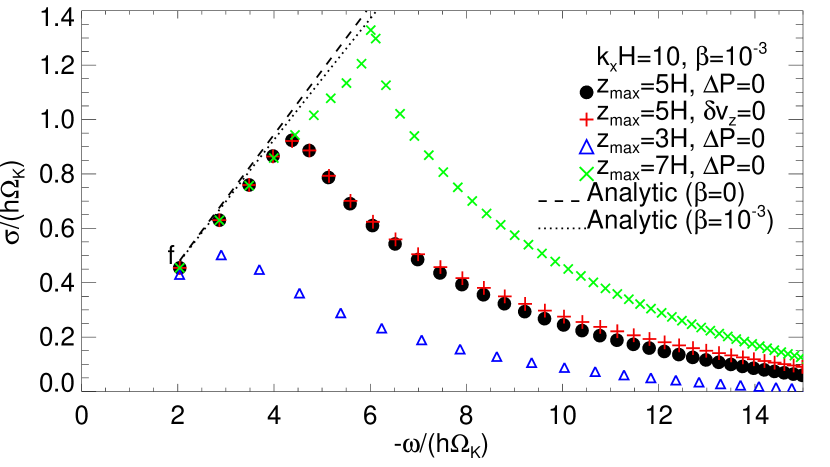
Figure 4.— Growth rate, $\sigma$, vs. oscillation frequency, $\omega$, for VSI modes with wavenumber $k_{x}=\hat{k}/H=10/H$ in the fiducial disk model with rapid cooling, $\beta=10^{-3}$. We investigate the effect of vertical box size, from $z_{\mathrm{max}}=3H$ (blue triangles) to $7H$ (green x’s) with a free surface boundary ($\Delta P=0$). For $z_{\mathrm{max}}=5H$ (black dots) we also compare free surface (black dots) and rigid (red plusses), finding little difference. The fundamental mode is marked by ‘f’. Lines show the analytic predictions for isothermal perturbations ($\beta=0$, dashed) and for $\beta=10^{-3}$ (dotted). See text for discussion.

6.1. Rapid thermal relaxation

We first calculate the VSI in a disk with rapid thermal relaxation by setting $\beta=10^{-3}$. Since $\beta\ll\beta_{\mathrm{crit}}$, this case gives similar results to the well studied case of isothermal perturbations (e.g. ; ; , ). This case allows us to explore and test our finite cooling time model in a familiar context.

Figure 5.— Pseudo-enthalpy perturbation $W$ (top) and vertical velocity perturbation $\delta v_{z}$ of the fundamental VSI with $\hat{k}=10$ in the fiducial disk with rapid thermal relaxation $\beta=10^{-3}$. The real (imaginary) parts of $W$ and $\delta v_{z}$ are plotted as solid (dotted) lines.

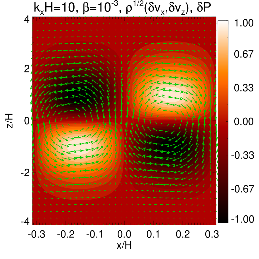
Figure 6.— Visualization of the fundamental VSI mode in Fig. 5. For this plot the mode has been transformed back to real space. Thus, the color scale corresponds to the real pressure perturbation scaled by its maximum value. Arrows show the real meridional flow multiplied by $\sqrt{\rho}$. The horizontal axis has been stretched for clarity.

6.1.1 Case study: $\hat{k}=10$

Fig. 4 maps the growth rates $\sigma$ and wave frequencies $\omega$ of unstable modes for $\hat{k}=10$. Each symbol corresponds to a different order mode, i.e. a different number of vertical node crossings. Lower order modes have smaller $|\omega|$ for fixed radial wavenumber, as expected for inertial-gravity waves (see §C.2.1).

We compare our numerical results to the analytic dispersion relations for $\beta=0$ and $10^{-3}$, from Eqs. C16 and 44, respectively. The analytic models also have discrete modes, which lie on the continuous curves that are plotted for clarity in Fig. 4. While the analytic models have many simplifications, they crucially lack an artificial vertical surface (as they assume an infinite vertical domain).

For our fiducial case (black dots), the lower order and lower frequency modes closely follow the analytic prediction with growth rates increasing with $|\omega|$. However, for $|\omega|\gtrsim 4h\Omega_{\rm K}$ the growth rate declines with $|\omega|$. This break from the analytic prediction is not due the choice of boundary condition, as we demonstrate by considering rigid boundaries (red plusses).

Rather, the decline in growth rate for high order models is due to the vertical box size, as seen by comparing the $z_{\mathrm{max}}/H=3,5$ and 7 cases in Fig. 4. Increasing $z_{\mathrm{max}}$ give better agreement with the analytic theory, which have $z_{\mathrm{max}}\to\infty$. Larger boxes include regions of larger vertical shear (see Eqs. 2 and 20), which higher order modes can tap to give larger growth rates. For the $z_{\mathrm{max}}=7H$ case, we begin to see another branch of modes with the highest growth rates at $\omega\sim-6h\Omega_{\rm K}$. This branch contains the ‘surface modes’ described below.

The need for vertically extended domains to capture the largest VSI growth rates is problematic, especially for hydrodynamic simulations. This complication is mitigated by at least two factors. First, we show below that with slower cooling, the growth of higher order modes is preferentially damped, consistent with the analysis in §5.3. Second, the fastest growing modes may not dominate transport when they operate in very low density surface layers, i.e. at many $H$. Quantifying which modes will contribute most to non-linear transport is an important issue, but beyond the scope of this work.

Fig. 5 shows eigenfunctions $W=\delta P/\rho$ and $\delta v_{z}$ for the lowest order fundamental mode. (In this and similar plots below, we normalize eigenfunctions such that its maximum amplitude is unity with vanishing imaginary part at the lower boundary.) Fig. 6 maps the pressure perturbation and meridional flow, scaled by $\sqrt{\rho}$ to reflect the contribution to kinetic energy. Notice the stretched $x$ axis. Radial velocities are in fact typically much smaller than vertical velocities, as expected for a vertically elongated, anelastic mode (N13). Most of the kinetic energy is contained within $\sim 2H$ of the midplane due to the density stratification.

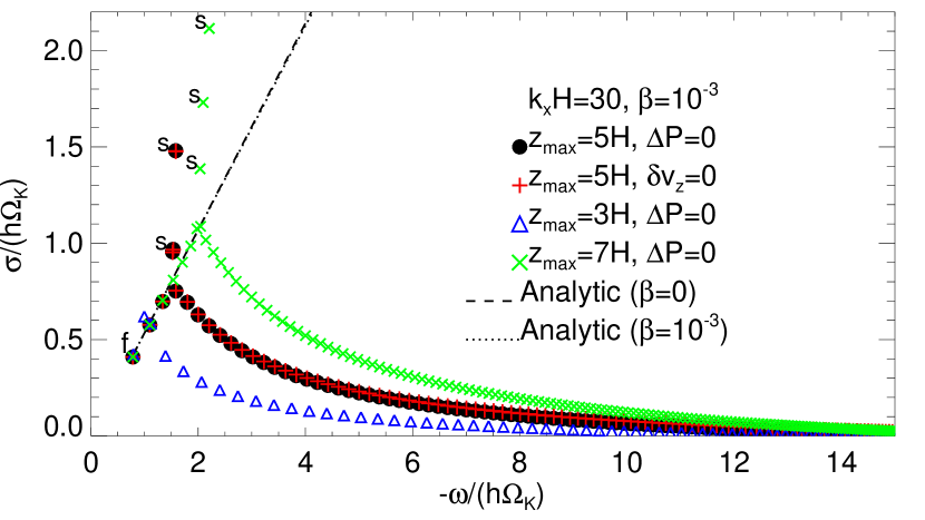
Figure 7.— Same as Fig. 4 but for $\hat{k}=30$. Examples of surface modes are marked by ‘s’.

Figure 8.— Example of a ‘surface mode’ in the fiducial disk model.

6.1.2 Surface modes of the VSI

The surface modes mentioned above are more prominent for larger wavenumbers. Fig. 7 maps the $\hat{k}=30$ eigenvalues, with the surface modes labeled. Surface modes strongly depend on the location of the imposed vertical boundary, and disagree with the analytic models, which lack an imposed surface. We thus discount the physical significance of surface modes for our model, as we explain further below.

Surface modes are a well known feature of the VSI in finite vertical domains (; ). BL15 show that surface modes arise whether the surface is imposed (as in our models) or natural (for disk models with a zero-density surface). BL15 mention the interface between a disk’s interior and corona as a physical boundary that can trigger surface modes. Since vertically isothermal disk models lack a surface, modes which depend on the adopted value of $z_{\mathrm{max}}$ are not physically meaningful.

The possibility of artificial surface modes seeding growth in numerical simulations of the VSI merits further study. Indeed N13 find that the initial growth of perturbations primarily occurs near the vertical boundaries. The motion in surface modes is indeed concentrated near the surface, as shown in Fig. 8, where the density is low. Thus, their contribution to transport might (by themselves) be weak, following the arguments in §6.1.1. Moreover surface modes, like all modes with large wavenumbers, are more prone to viscous damping, as discussed in §8.1.

While the relatively large growth rates of surface modes is tantalizing, we dismiss them in disk models that lack a physical surface.

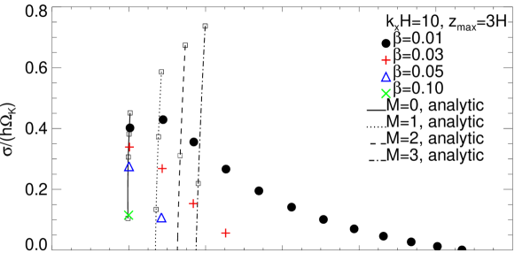
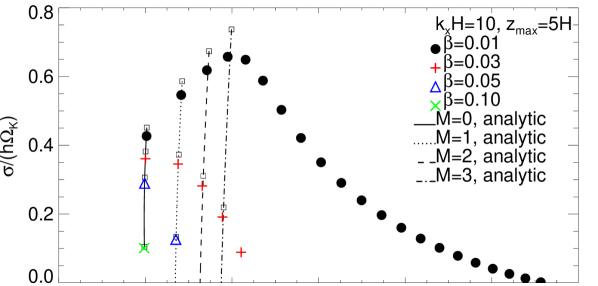
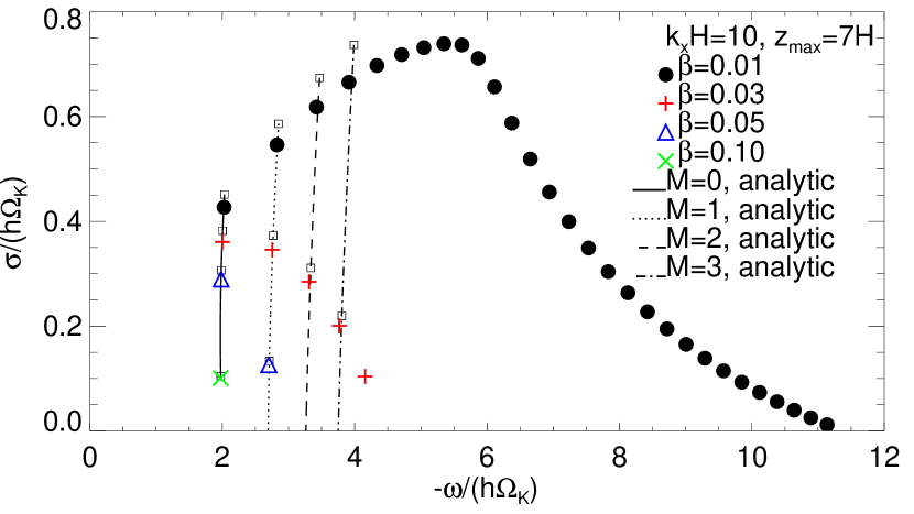
Figure 9.— Unstable modes with $\hat{k}=10$ and thermal relaxation timescales $\beta=0.01$ (black dots), $\beta=0.03$ (red crosses), $\beta=0.05$ (blue triangles) and $\beta=0.1$ (green crosses); for different vertical domain sizes $z_{\mathrm{max}}=3H$ (top), $z_{\mathrm{max}}=5H$ (middle, the fiducial setup) and $z_{\mathrm{max}}=7H$ (bottom). Lines are computed from Eq. 44 for $M=0$ (solid, fundamental mode) and $M=1,\,2,\,3$ (dotted, dashed, dash-dot, respectively). Along each line, $\beta$ increases continuously from $0.01$ to $0.1$ from top to bottom, and squares mark corresponding $\beta$ values with numerical results.

6.2. Slower thermal relaxation

We now consider the effect of longer cooling timescales by gradually increasing $\beta$. We expect VSI growth for $\beta<\beta_{\mathrm{crit}}=0.125$. We also expect that higher order modes will damp at even lower $\beta$ values, as argued in §5.3.

Fig. 9 largely confirms these expectations by plotting eigenvalues for $\hat{k}=10$ and $\beta$ from $0.01$ to $0.1$. The analytic results from Eq. 44 are now plotted as different curves for each mode order $M$, with $\beta$ varying along each curve. We see the standard increase in frequency, $|\omega|$, with mode order.

As expected, the higher order modes are preferentially damped. For $\beta\geq 0.03$ the fundamental ($M=0$) mode is the fastest growing. For $\beta=0.1$, only the $M=0$ mode grows. This growth is slow since $\beta$ is near $\beta_{\mathrm{crit}}$.

Fig. 9 also shows how cooling times affect the dependence on $z_{\mathrm{max}}$, the size of the vertical domain. For all cooling times, the fundamental mode depends only weakly on $z_{\mathrm{max}}$, and there is good agreement with analytic values. This convergence is reassuring given the importance of the fundamental mode at longer cooling times. For higher order modes and short cooling times, however, the eigenvalues vary strongly with $z_{\mathrm{max}}$. The disagreement with analytic theory is strongest for the smallest domain, with $z_{\mathrm{max}}=3H$. For $\beta\geq 0.03$, the $z_{\mathrm{max}}/H=5,7$ and the analytic results are well converged (aided by the fact that only $M<5$ modes grow).

Figure 10.— Same as Fig. 5 but with a thermal relaxation timescale $\beta=0.1$.

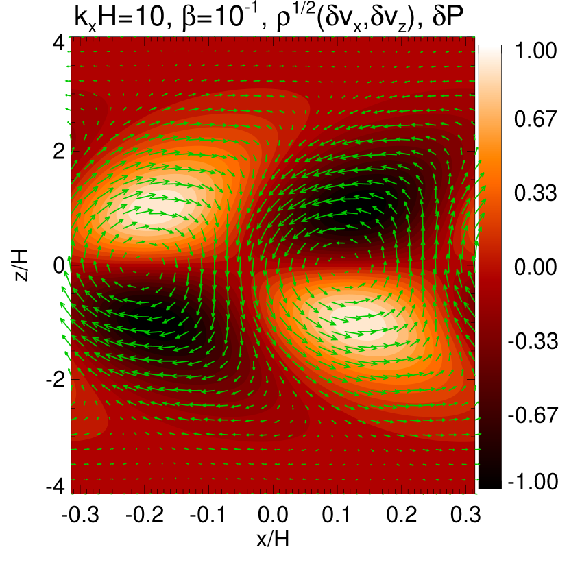
Figure 11.— Same as Fig. 6 but with a thermal relaxation timescale $\beta=0.1$.

Figures 10 and 11 illustrate the eigenfunction of the fundamental mode with $\hat{k}=10$ and $\beta=0.1$. Compared with the small $\beta$ case in Figs. 5 and 6, the eigenfuctions show a more complex variation of phase with height. This dependence yields the ‘tilted’ appearance of pressure field in Fig. 11. Physically, the increased role of buoyancy, which increases with height, explains why larger $\beta$ values produce more complex vertical structure.

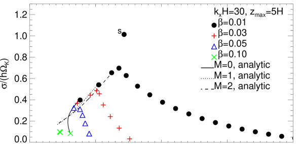
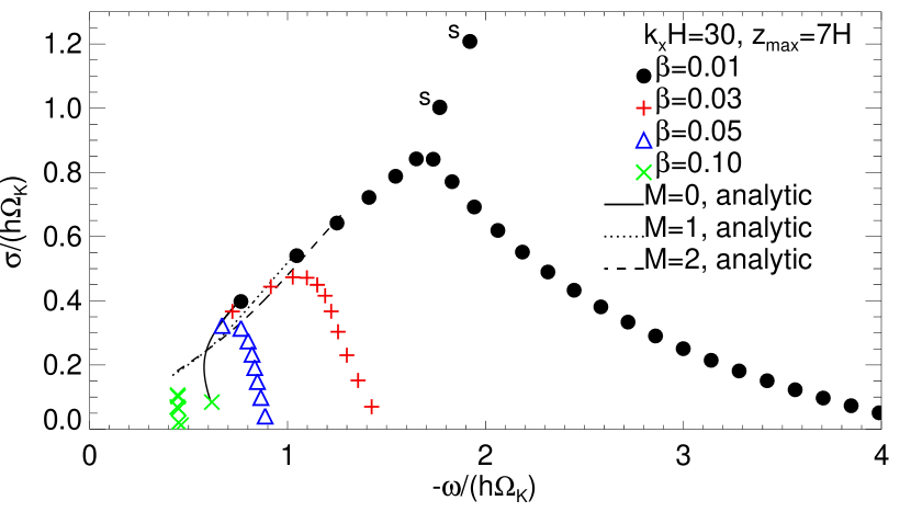
Figure 12.— Same as Fig. 9 but for $\hat{k}=30$ and domain sizes $z_{\mathrm{max}}=5H$ (top) and $7H$ (bottom). Examples of surface modes are marked with ‘s’.

Fig. 12 shows how cooling affects higher wavenumber modes, specifically $\hat{k}=30$. We only show the larger domains with $z_{\mathrm{max}}=5H,7H$. These cases again show good convergence for $\beta\geq 0.03$, which the smaller domain with $z_{\mathrm{max}}=3H$ lacks.

With slower cooling, the wave frequency shows a more complex dependence on mode order, both analytically and numerically. For $\beta=0.1$, the fundamental mode (which lies on the $M=0$ curve) no longer has the smallest $|\omega|$ value.

Moreover, the fundamental mode is no longer the fastest growing mode for $\beta\geq 0.03$, or even for $\beta=0.1$. This complication is not actually surprising since $|hq\hat{k}|=1.5$ is no longer less than unity, as required in the analytic derivation of §5.3. Though inconvenient, given that the fundamental mode is easy to identify and the most numerically converged, this complication is not ultimately significant for the operability of the VSI.

Fig. 12 also demonstrates that artificial surface modes are damped for $\beta\geq 0.03$. We are thus confident that artificial surface modes should not affect our determination of the critical cooling time.

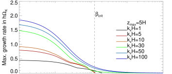
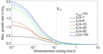
Figure 13.— Maximum VSI growth rates in the fiducial disk model as a function of the thermal relaxation timescale $\beta$, for $z_{\mathrm{max}}=5H$ (top) and $z_{\mathrm{max}}=7H$ (bottom). The vertical line is the critical thermal timescale $\beta_{\mathrm{crit}}$ obtained from Eq. 46.

6.3. Critical thermal relaxation timescale

Having explored the behavior of VSI modes with cooling, we turn to the numerical validity of the analytic cooling criterion for vertically isothermal disks, $\beta<\beta_{\mathrm{crit}}=h|q|/(\gamma-1)$.

Fig. 13 shows how VSI growth rates vary with cooling time in our fiducial model with $\beta_{\mathrm{crit}}=0.125$. Curves are for a fixed horizontal wavenumber, and show the maximum growth rate for all vertical mode orders. The discontinuity in some curves occurs when the fastest growth switches to a different mode order.

For $\hat{k}=5,10$, the growth rate drops to zero at the expected $\beta=\beta_{\mathrm{crit}}$. For longer wavelength modes, with $\hat{k}=1$, growth persists to slightly longer cooling times. This difference is not surprising since our analytic derivation assumed $\hat{k}^{2}\gg 1$, but the change is quantitatively minor.

For shorter wavelengths, with $\hat{k}\geq 30$, growth persists for $\beta$ significantly larger than $\beta_{\mathrm{crit}}$. This tail of growth is partly explained by the breaking of the $\hat{k}<1/|qh|=20$ approximation, used in the analytic derivation. Despite the lack of a clear stability boundary at high $\hat{k}$, the $\beta_{\mathrm{crit}}$ threshold remains useful, since growth rates drop to $\lesssim 10\%$ of their maximum value at $\beta_{\mathrm{crit}}$ and continue to fall for larger $\beta$. Moreover, we expect that longer wavelength modes with $\hat{k}\lesssim 20$ are more significant for disk transport, see §8.1.

Comparing the $z_{\mathrm{max}}/H=5,7$ cases in Fig. 13, we see that the location of the vertical boundary has little effect on the critical cooling time. This agreement occurs despite the fact that peak growth rates differ as $\beta\to 0$. We are thus confident that boundary effects, including surface modes, do not affect our analysis of the critical cooling time.

Our results agree with the vertically isothermal simulations of N13 which used the same disk parameters as our fiducial model. The expected $\beta_{\mathrm{crit}}=0.125$ is consistent with the simulations shown in their Fig. 12. N13 found nonlinear VSI growth for $\beta=0.06<\beta_{\mathrm{crit}}$ but no growth for $\beta=0.6>\beta_{\mathrm{crit}}$.

Figure 14.— Dependence of the upper limit to the thermal relaxation timescale $\beta_{\mathrm{crit}}$ for the fundamental VSI mode on disk parameters. The fiducial setup is $(\gamma,\Gamma=(1.4,1.011)$ and $(p,q,h)=(-1.5,-1,0.05)$. Top: varying $q\in[-1.2,-0.2]$; middle: varying $\gamma\in[1.2,2.0]$; bottom: varying $h\in[0.02,0.1]$. The perturbation wavenumber is $\hat{k}=10$.

Fig. 14 confirms that the numerically determined $\beta_{\mathrm{crit}}$ shows the expected scaling with disk parameters $h$, $q$, and $\gamma$. For this test we fix $\hat{k}=10$ (an appropriate value for all the reasons discussed above) and measure the smallest $\beta$ value where growth vanishes. The agreement with the analytic scaling of Eq. 46 is quite good, confirming the applicability of our critical cooling time in vertically isothermal disks.

6.4. Vertically non-isothermal disk model

We now generalize our critical cooling time by considering disks which are not vertically isothermal. We rely on physical arguments for this generalization. In disks with weaker vertical stratification, i.e. $\Gamma>1$ for fixed $\gamma$, we expect $\beta_{\mathrm{crit}}$ to be larger. We thus transform $1/(\gamma-1)\to 1/(\gamma-\Gamma)$.

We also expect $\beta_{\mathrm{crit}}$ to scale with the vertical shear. In general the vertical shear rate $\partial_{z}\Omega\propto s$, the radial entropy gradient, see Eq. 20. We thus transform $q\to s=q+p(1-\Gamma)$.

Our estimate for the generalized cooling time criterion — valid for both vertically isothermal and non-isothermal disks (cf. Eq. 46) — is thus

$$\beta_{\mathrm{crit}}\to\beta_{\mathrm{crit,gen}}=\frac{h|s|}{\gamma-\Gamma}.$$ (48)

We test $\beta_{\mathrm{crit,gen}}$ using a disk model with $(p,q,h)=(-0.5,-1,0.05)$ and $(\gamma,\Gamma)=(1.4,1.3)$. For this setup, $s=-0.85$ and $\beta_{\mathrm{crit,gen}}=0.425$, which is $\sim 3$ times larger than our fiducial, vertically isothermal disk with $\beta_{\mathrm{crit}}=0.125$.

We set the vertical domain size just inside the physical, zero-density disk surface, $z_{\mathrm{max}}=0.99H_{s}\simeq 2.6H$, see Eq. 16. At this surface, the vertical buoyancy frequency, $N_{z}$, diverges as $|z|\to H_{s}$. While we might expect pathological behavior for this model, we fortunately do not find it.

In Fig. 15 we plot the mode diagram for $\hat{k}=30$ and several values of $\beta$. This plot is qualitatively similar to the vertically isothermal case, Fig. 9. As before, larger $\beta$ values rapidly stabilize higher order modes. For sufficiently large $\beta$ only the fundamental mode is unstable, with a growth rate that decreases as $\beta$ approaches $\beta_{\mathrm{crit,gen}}$.

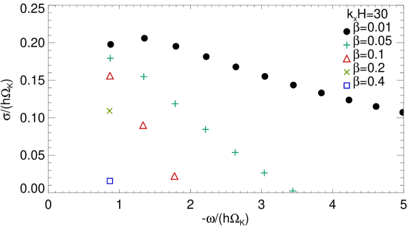
Figure 15.— Unstable modes in a vertically non-isothermal disk with $\hat{k}=30$ and a range of thermal relaxation timescales.

Fig. 16 shows how maximum VSI growth rates vary with $\beta$ in the vertically non-isothermal model. The qualitative behavior is similar to Fig. 13 for the vertically isothermal disk. For $\hat{k}=O(10)$, growth rates drop to zero at the predicted $\beta_{\mathrm{crit,gen}}$. As in the vertically isothermal case, modes with both lower and higher wavenumbers exhibit slow growth rates beyond the critical cooling time. As argued in §6.3, the critical cooling time is useful despite not being an absolute stability limit.

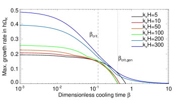
Figure 16.— Maximum VSI growth rates in the vertically non-isothermal disk model as a function of the thermal relaxation timescale $t_{c}=\beta\Omega_{\rm K}^{-1}$. The vertical dashed line is the critical thermal timescale given by Eq. 46. A conjectured critical thermal timescale accounting for a non-isothermal background, given by $\beta_{\mathrm{crit,gen}}=0.425$ (see Eq. 48), is also shown as the vertical dotted line.

The generalized cooling time criterion in Eq. 48 thus appears to be valid. If a disk’s vertical structure is not characterized by a single polytropic index, $\Gamma$, we expect that a density weighted average of $\beta_{\mathrm{crit,gen}}$ should be a good approximation. This expectation remains to be tested.

7. The VSI with realistic protoplanetary disk cooling

To this point we have treated the cooling time, $\beta$, as a free parameter that, moreover, is independent of height. To understand the applicability of the VSI to PPDs, we now consider $\beta$ values that are consistent with PPD models. Section 7.1 develops our PPD cooling law, which depends on disk radius, disk height and perturbation wavelength. We compare these PPD $\beta$ values to $\beta_{\rm crit}$ in §7.2. While this comparison is instructive, it is not complete since $\beta_{\rm crit}$ was derived assuming a vertically constant $\beta$. Thus in §7.3 we analyze the linear growth of VSI with our PPD $\beta$ values.

7.1. Cooling model

7.1.1 Radiative diffusion and Newtonian cooling

The thermal relaxation of a perturbation depends on the relative sizes of the perturbation’s lengthscale, $l$, and the photon mean-free-path,

$$l_{\mathrm{rad}}\equiv\frac{1}{\kappa_{d}\rho}$$ (49)

where $\kappa_{d}$ is the opacity, specifically the dust opacity appropriate for cold PPDs.

In the optically thick limit, $l\gg l_{\mathrm{rad}}$, radiative diffusion smooths out thermal perturbations. In this regime, the linearized cooling function is

$$\delta\Lambda_{\mathrm{diff}}=\frac{P}{\rho TC_{v}}\nabla\cdot\left(k_{\mathrm{rad}}\nabla\delta T\right),$$ (50)

where $k_{\mathrm{rad}}$ is the radiative conduction coefficient defined below, and $C_{v}$ is the specific heat capacity at constant volume.

Since the VSI is characterized by vertically-elongated, radially-narrow disturbances, we retain only the radial derivatives of the perturbations in Eq. 50. Thus, in the radially local approximation, we have

$$\delta\Lambda_{\mathrm{diff}}\simeq-\eta k_{x}^{2}P\frac{\delta T}{T},$$ (51)

where the radiative diffusion coefficient is

$$\eta\equiv{k_{\mathrm{rad}}\over\rho C_{v}}=\frac{16\sigma_{s}T^{3}}{3\kappa_{d}\rho^{2}C_{v}},$$ (52)

and $\sigma_{s}$ is the Stefan-Boltzmann constant. The thermal relaxation timescale (defined in Eq. 10) for radiative diffusion is thus

$$t_{\mathrm{diff}}=\frac{1}{\eta k_{x}^{2}}.$$ (53)

In the optically thin regime, $l\ll l_{\mathrm{rad}}$, thermal relaxation operates by ‘Newtonian cooling’. The cooling time is independent of $l$ and inversely proportional to the opacity, $t_{\mathrm{thin}}\propto 1/\kappa_{d}$. Specifically

$$t_{\mathrm{thin}}=\frac{l_{\mathrm{rad}}^{2}}{3\eta},$$ (54)

and $t_{\mathrm{thin}}$ does not depend on $\rho$ (because our adopted $\kappa_{d}$ depends on $T$ only, see below).

Our general cooling time for all perturbations,

$$t_{c} \equiv t_{\mathrm{thin}}+t_{\mathrm{diff}},$$ (55)

is a simple prescription to smoothly match the optically thick and thin limits.

7.1.2 PPD cooling times

In a vertically isothermal disk with surface density $\Sigma=\rho_{0}\sqrt{2\pi}H$, the dimensionless thermal relaxation time $\beta$ becomes

$$\beta(r,z;\hat{k})\equiv t_{c}\Omega_{\rm K}=\frac{\Sigma^{2}\Omega_{\rm K}}{\eta\rho^{2}}\left[\frac{1}{3\kappa_{d}^{2}\Sigma^{2}}+\frac{\hat{\rho}^{2}(z)}{2\pi\hat{k}^{2}}\right].$$ (56)

where $\hat{\rho}=\rho/\rho_{0}$. The first and second terms in square brackets represent the optically thin and thick cooling regimes, respectively.

We adopt the Minimum Mass Solar Nebula (MMSN) disk model of Chiang & Youdin (2010) which specifies

$$\Sigma =2200r_{\mathrm{AU}}^{-3/2}\mathrm{g}\,\mathrm{cm}^{-2},$$ (57a)

$$T =120r_{\mathrm{AU}}^{-3/7}\mathrm{K},$$ (57b)

with $r_{\mathrm{AU}}\equiv r/\mathrm{AU}$. This model has $q=-3/7$, $p=-39/14$ and $h=0.022r_{\mathrm{AU}}^{2/7}$, using $\mu=2.33$ and the above relation between $\Sigma$ and $\rho_{0}\propto r^{p}$.

For the dust opacity we adopt the Bell & Lin (1994) law with $\kappa_{d}\propto T^{2}$, giving

$$\kappa_{d}=2.88\hat{\kappa}_{d}r_{\mathrm{AU}}^{-6/7}\mathrm{cm}^{2}\,\mathrm{g}^{-1},$$ (58)

where the opacity normalization factor, $\hat{\kappa}_{d}$, scales with the ratio of small dust to gas; $\hat{\kappa}_{d}=1$ is our fiducial case.

For this disk and opacity model, the cooling time becomes

$$\beta(r,z;\hat{k})= 3.9\times 10^{-3}\hat{\kappa}_{d}^{-1}r_{\mathrm{AU}}^{9/14}$$

$$\times\left[1+1.9\times 10^{7}\hat{\kappa}_{d}^{2}\hat{\rho}^{2}(z)r_{\mathrm{AU}}^{-33/7}\hat{k}^{-2}\right].$$ (59)

Perturbations are in the optically thin regime for

$$\hat{k}\gtrsim 2.5\times 10^{3}\hat{\kappa}_{d}\hat{\rho}(z)r_{\mathrm{AU}}^{-33/14}.$$ (60)

In the inner disk, e.g. $r_{\mathrm{AU}}\sim 1$, only extremely small-scale perturbations are in the optically-thin regime near the midplane. However, in the outer disk, e.g. $r_{\mathrm{AU}}\sim 10$, more moderate wavenumbers $\hat{k}\gtrsim 10$ experience optically-thin cooling.

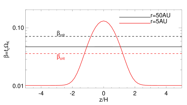
Figure 17.— Thermal relaxation timescales in the fiducial MMSN at $r=50$AU and $r=5$AU for $\hat{k}=30$ (solid lines). The corresponding horizontal dashed lines are the critical thermal relaxation timescales derived in linear theory.

Figure 18.— Dimensionless thermal relaxation timescales $\beta$, evaluated at the midplane (left) and at $z=3H$ (right) in the fiducial PPD. Eq. 7.1.2 is plotted for three values of the perturbation radial wavenumber: $\hat{k}=1$ (dotted), $\hat{k}=10$ (dashed) and $\hat{k}=100$ (dashed-dot), for three values of the opacity relative to the MMSN: $\hat{\kappa}_{d}=0.1$ (top), $\hat{\kappa}_{d}=1$ (middle) and $\hat{\kappa}_{d}=10$ (bottom). The solid line is the critical thermal relaxation timescale $\beta_{\mathrm{crit}}$.

7.2. $\beta$ vs. $\beta_{\mathrm{crit}}$ in PPDs

The simplest way to estimate whether the VSI can operate at a given radius in a PPD is to compare the cooling time (Eq. 7.1.2) to its critical value (Eq. 46), evaluated for the MMSN as

$$\beta_{\mathrm{crit}}=0.024r_{\mathrm{AU}}^{2/7}.$$ (61)

This comparison is strictly valid only for optically thin cooling which is independent of height, as assumed in the derivation of $\beta_{\mathrm{crit}}$. This condition typically holds in the outer disk. Fig. 17 shows that a $\hat{k}=30$ perturbation at 50AU has vertically constant $\beta$. Furthermore, since $\beta<\beta_{\mathrm{crit}}$, the disturbance would be unstable.

For optically thick cooling, $\beta$ varies with height, complicating the comparison with $\beta_{\mathrm{crit}}$. At 5AU, Fig. 17 shows that cooling times are long in the midplane with $\beta>\beta_{\mathrm{crit}}$. However, since $\beta<\beta_{\mathrm{crit}}$ away from the midplane, we require the analysis of §7.3 to determine if the VSI can grow. (That calculation will show that growth is strongly suppressed for this case.) We proceed with the awareness that optically thick regions in the inner disk are a complication, but that we can reasonably expect VSI growth if $\beta<\beta_{\mathrm{crit}}$ at all heights.

In Fig. 18, we compare $\beta$ to $\beta_{\mathrm{crit}}$ across a range of disk radii for different heights, opacity values and wavenumbers. For optically thin cooling in the outer disk, curves for different wavenumbers overlap, as expected from Eq. 7.1.2. Since the (optically thin) slope of $\beta$ is steeper than for $\beta_{\mathrm{crit}}$, VSI growth can be suppressed at large radii (for the chosen opacity law). This effect is seen for $\hat{\kappa}_{d}=1$ in the central panels of Fig. 18, where VSI is damped outside $\sim 150$ AU.

We find that the most important factor for VSI growth is the opacity. With a smaller opacity, $\hat{\kappa}_{d}=0.1$, growth is suppressed at all radii, as shown in the top panels of Fig. 18. Since optically thin cooling is too slow in this case, optically thick cooling — above the floor set by optically thin cooling — is also too slow.

Larger opacities make optically thin cooling much faster than $\beta_{\mathrm{crit}}$, as shown in the top panels of Fig. 18. However with larger opacities, optically thick cooling affects larger disk radii, slowing the cooling. Remarkably, the adopted MMSN value of opacity hits the a sweet spot where optically thin cooling is fast enough, yet slower optically thick can be restricted to inner disk radii.

At smaller disk radii, Fig. 18 shows the hallmark of diffusive cooling, that larger wavenumbers can cool faster, but not below the floor set by optically thin cooling. Optically thick cooling times also rise sharply toward smaller radii (as $\beta\propto r^{-57/14}$) due to high densities and short orbital times. This effect suppresses VSI growth at small radii, but with a strong wavenumber dependence.

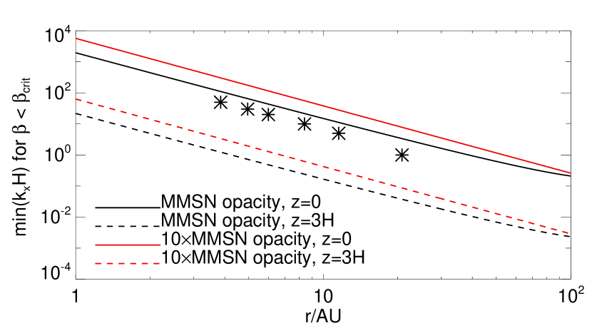
Figure 19.— The minimum perturbation wavenumber $\hat{k}$ in the MMSN such that the associated dimensionless thermal relaxation time $\beta$ at $z=0$ (solid) and $z=3H$ (dashed) is less than the critical timescale $\beta_{\mathrm{crit}}$. Asterisks correspond to the inner cut-off radii shown in Fig. 20.

Fig. 19 highlights this wavenumber dependence by plotting the wavenumbers for which $\beta=\beta_{\mathrm{crit}}$. Above the solid curves (i.e. for larger wavenumbers), $\beta<\beta_{\mathrm{crit}}$ at all disk heights, implying linear VSI growth. Below the dashed curves, VSI growth is strongly suppressed since $\beta>\beta_{\mathrm{crit}}$ for all $|z|<3H$. Between the solid and dashed curves some growth is possible, but only fairly close to the solid curve (according to §7.3). Thus linear growth of the VSI near 1 AU is only possible if $k_{x}\gtrsim 10^{3}/H$. As argued elsewhere, such small-scale disturbances may not drive significant turbulence or transport.

We thus doubt that the VSI is significant at 1 AU in MMSN-like PPDs, for any opacity. At higher opacities, the required wavenumbers become shorter and even more problematic, as shown by the red curves in Fig. 19. At lower opacities, even optically thin cooling (the fastest possible) is too slow, as discussed above.

7.3. VSI growth in the MMSN

We now consider the growth of the VSI in a MMSN disk model. This numerical calculation is similar to §6 but with different disk parameters and with the self-consistent cooling times of Eq. 7.1.2.

We consider the growth timescales of the fundamental mode for a range of wavenumbers and disk radii. We focus on the fundamental, i.e. lowest order vertical, mode because it is the fastest growing mode except for some surface modes at high wavenumbers. We neglect these surface modes for reasons discussed in §6 and §8.1.

Fig. 20 shows that in the MMSN, the VSI is active from $r_{\mathrm{AU}}\sim 5$ to $r_{\mathrm{AU}}\sim 50$ with growth timescales $\sim 30$—40 orbits. A small radius cut-off exists, inside of which growth is strongly suppressed. The cut-off occurs at smaller radii for larger wavenumbers, as expected from Fig. 19. Growth at smaller disk radii is possible for yet larger wavenumbers, but we remain skeptical about the non-linear significance of such short lengthscales.

The growth times rise gradually as $r$ increases towards 100AU in Fig. 20. This trend is expected as the outer radius cutoff at $\sim 150$AU (from Fig. 18) is approached. Our numerical results suggest the VSI is efficient at radii of few tens of AU in the MMSN, consistent with estimates made by N13 using the same disk model.

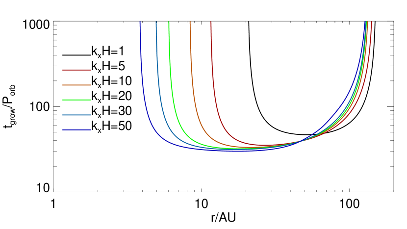
Figure 20.— VSI growth times ($t_{\rm grow}=1/\sigma$) in orbital units ($P_{\mathrm{orb}}=2\pi/\Omega_{\rm K}$) for the reference MMSN disk model with self-consistent dust cooling.

8. Caveats and Neglected Effects

8.1. Viscosity

Our neglect of viscosity is valid in a laminar disk, because molecular viscosity is so small. However, turbulence could act as an effective viscosity which preferentially damps small scale modes. Since the goal of VSI is to drive turbulent transport, the most relevant modes for sustaining the VSI should be able to overcome turbulent damping.

To roughly estimate the wavelengths which are prone to damping, we consider the standard prescription for the kinematic viscosity $\nu=\alpha c_{s}H$ (Shakura & Sunyaev, 1973), in terms of the dimensionless $\alpha$ parameter. The viscous timescale for a perturbation lengthscale $l\sim 1/k_{x}=H/\hat{k}$ is $t_{\mathrm{visc}}=1/\alpha\hat{k}^{2}\Omega$. For significant growth, $t_{\mathrm{visc}}$ should be longer than the characteristic VSI growth timescale $1/(h|q|\Omega)$, i.e. $\hat{k}^{2}\lesssim|q|h/\alpha$. With $h\sim 0.05$, $q=-1$ and $\alpha$ from simulations (N13), we estimate that growth requires $\hat{k}\lesssim 20$ for $\alpha\sim 10^{-4}$ or $\hat{k}\lesssim 70$ for $\alpha\sim 10^{-5}$.

This argument justifies our focus on moderate wavenumbers, $\hat{k}=O(10)$. Future work should consider the viscous effects in more detail, to better understand how the VSI operates in nature and in simulations.

8.2. Convective overstability

The VSI bears some similarity to the ‘convective overstability’ (CONO, Klahr & Hubbard, 2014; Lyra, 2014). Both instabilities rely on thermal relaxation to overcome the stability of disks to adiabatic perturbations, i.e. the Solberg-Hoiland criteria (see §3.4).

The key differences are that the CONO neglects vertical buoyancy and requires an imaginary horizontal buoyancy,

$$N_{r}^{2}\equiv-{1\over\rho C_{P}}{\partial P\over\partial r}{\partial S\over\partial r}<0\,.$$ (62)

Since vertical buoyancy is an important stabilizing influence for the VSI, it should be considered in future studies of CONO.

The sign of $N_{r}^{2}$ depends on disk parameters. To demonstrate that the parameters needed for $N_{r}^{2}<0$ are somewhat extreme, or at least non-standard, we consider the midplane of vertically isothermal disks with $\Sigma\propto r^{n}$ so that $n=p+q/2+3/2$. Using Eqs. 22a and 62 with $\gamma=1.4$, $N_{r}^{2}<0$ requires $n>3(1/2+q)$. For standard disk temperature laws, this requirement implies a flat or rising surface density profile, e.g. $n=3/14$ for $q=-3/7$ or $n=0$ for $q=-1/2$. Since standard $\Sigma$ profiles decline with radius, CONO is most like to operate at special locations, like the outside edges of disk gaps or holes and/or shadowed regions where $q<-1/2$.

Perhaps due to these physical differences, CONO operates in different regimes of parameter space than the VSI. The CONO grows best for longer wavelengths $\hat{k}\lesssim 1$ and longer cooling times $\beta\sim 1$.

Future work should aim to understand these related instabilities in the same framework, thereby explaining the key differences.

8.3. Radiative transfer

Our relatively simple treatment of cooling with an idealized dust opacity could certainly be generalized in future works. In hotter disks, gas phase opacities must be considered. In cold disks, there are many choices for the dust opacity, which varies with grain sizes and compositions. Changing dust properties would alter the viability of the VSI for better or worse. The radiative transfer itself could be calculated with higher levels of sophistication, as is already being done in numerical simulations of the VSI (Stoll & Kley, 2014).

9. Summary and discussion

In this paper we study the vertical shear instability (VSI) with a focus the role of radiative cooling. In turn we assess the viability of the VSI as an angular momentum transport mechanism in protoplanetary disks (PPDs).

Our linear, axisymmetric analysis of the VSI considers (uniquely to our knowledge) finite cooling times in a vertically global model. In order for vertical shear to drive the VSI, short cooling times are needed to weaken the stabilizing effects of vertical buoyancy. Our main analytical finding, which we confirm numerically, is the critical cooling timescale above which VSI growth is suppressed, Eqs. 5 and 46.

Our main focus is irradiated, vertically isothermal disks which have strong vertical buoyancy. The critical cooling time is thus short, shorter than the orbital time by a factor of the disk aspect ratio. This finding is consistent with, and helps explain, the results of recent numerical simulations (N13). We briefly consider vertically non-isothermal disks in §6.4.

In applying our results to PPDs, we pay particular attention to the transition from optically thick radiative diffusion to optically thin Newtonian cooling. The largest obstacle to VSI occurs in high density inner disk, $\lesssim 1$ – 5AU, where radiative diffusion times are slow. Shorter wavelength disturbances cool faster, so long as they remain optically thick. In the inner disk, however, our VSI cooling criterion requires wavelengths that are too short to drive significant transport. The best hope for the VSI in inner disk is a low surface density, which speeds radiative diffusion by lengthening the photon mean free path. This option naturally begs the question of what accretion mechanism lowered the surface density in the first place.

In the outer disk, the VSI tends to cool in the optically thin limit. The main issue is whether the opacity is high enough for optically thin cooling to be sufficiently fast. Our standard opacity assumes a Solar abundances of small dust. In this case, the VSI can operate from $\sim 5$ – 100AU. A factor of 10 reduction in the opacity, for instance by locking small dust into planetesimals and planetary cores (Youdin & Kenyon, 2013), makes cooling times too slow for VSI growth. In this case cooling is too slow not just in the outer disk, but into $<1$ AU.

An enhanced opacity makes optically thin cooling faster and radiative diffusion slower. This shift favors VSI growth in the outer disk at the expense of the inner disk, pushing the inner limit of VSI growth further out. The standard choice — corresponding to Solar abundances in a standard MMSN disk — allows the VSI to grow over the widest range of relevant disk radii.

Our detailed study of the spectrum of VSI modes confirms that some artificial ‘surface modes’ are triggered by imposed vertical boundaries (; ). Domain size convergence studies are thus essential. Fortunately, our results show that longer cooling times stifle the growth of surface modes. Thus, at least in some cases, more realistic radiative transfer also produces more reliable dynamics.

The VSI deserves further study as a viable mechanism to drive at least low levels of accretion in cold disks.

Appendix A Derivation of the approximate equations

Here we detail the derivation of Eq. 29 used in the analytical discussion of §5. Starting with Eqs. 27a — 27e, we set $\Gamma=1$ and $\zeta=0$ for the vertically isothermal limit and the fully-radially-local approximation, respectively. We eliminate the horizontal velocity perturbations ($\delta v_{x},\,\delta v_{y}$) to obtain

$$\mathrm{i}\upsilon\delta v_{z}=\frac{dW}{dz}+\frac{\partial\ln{\rho}}{\partial z}\left(W-Q\right),$$ (A1a)

$$\frac{\upsilon^{2}}{c_{s}^{2}}Q+\frac{\upsilon^{2}k_{x}^{2}}{D}W=\mathrm{i}\upsilon\left(\frac{\mathrm{i}k_{x}r}{D}\frac{\partial\Omega^{2}}{\partial z}-\frac{\partial\ln{\rho}}{\partial z}\right)\delta v_{z}-\mathrm{i}\upsilon\frac{d\delta v_{z}}{dz},$$ (A1b)

$$\upsilon^{2}W-\gamma\upsilon^{2}Q+\frac{\mathrm{i}\upsilon}{t_{c}}\left(W-Q\right)=\mathrm{i}\upsilon c_{s}^{2}\frac{\partial\ln{\rho}}{\partial z}\left(\gamma-1\right)\delta v_{z},$$ (A1c)

where

$$D\equiv\kappa^{2}-\upsilon^{2}.$$ (A2)

Reduction to a single ODE requires $\partial_{z}D=\partial_{z}\kappa^{2}$. At this point we could apply the low frequency and Keplerian approximations to set $D\rightarrow\kappa^{2}\rightarrow\Omega_{\rm K}^{2}$, then $D$ is vertically constant, and we can obtain Eq. 29 more directly. However, to demonstrate that the order of approximation is irrelevant, we will retain $\partial_{z}\kappa^{2}$ initially. Using Eq. 19—21,

$$\frac{\partial\kappa^{2}}{\partial z}=4\frac{\partial\Omega^{2}}{\partial z}+r\frac{\partial}{\partial r}\frac{\partial\Omega^{2}}{\partial z}=-\frac{d\ln\rho}{dz}\frac{qc_{s}^{2}}{r^{2}}\left(\frac{3z^{2}}{r^{2}+z^{2}}-1\right)\equiv-\frac{d\ln\rho}{dz}\frac{qc_{s}^{2}}{r^{2}}F(r,z).$$ (A3)

The function $F$ increases monotonically from $F=-1$ at $z=0$ to $F\to 2$ as $|z|\to\infty$, so $|F|=O(1)$.

We eliminate $W,\,Q$ from Eqs. A1, using Eqs. 31 and A3 to obtain

$$0= \frac{d^{2}\delta v_{z}}{dz^{2}}+\left[1+\frac{\mathrm{i}k_{x}c_{s}^{2}q}{Dr}-\frac{k_{x}^{2}c_{s}^{2}}{\left(k_{x}^{2}c_{s}^{2}+\chi D\right)}\frac{qc_{s}^{2}F}{Dr^{2}}\right]\frac{d\ln\rho}{dz}\frac{d\delta v_{z}}{dz}$$

$$+\left\{\upsilon^{2}\left(\frac{k_{x}^{2}}{D}+\frac{\chi}{c_{s}^{2}}\right)+\left(\chi+\frac{\mathrm{i}k_{x}c_{s}^{2}q}{Dr}\right)\frac{d^{2}\ln\rho}{dz^{2}}-\frac{c_{s}^{2}}{D}\left(\frac{d\ln\rho}{dz}\right)^{2}\left(k_{x}^{2}-\frac{\mathrm{i}k_{x}q}{r}\right)\left[\left(1-\chi\right)+\frac{\chi}{\left(k_{x}^{2}c_{s}^{2}+\chi D\right)}\frac{qc_{s}^{2}F}{r^{2}}\right]\right\}\delta v_{z},$$ (A4)

where we have replaced $\partial/\partial z$ by $d/dz$ for the fully-radially-local treatment. Now we make the low frequency and Keplerian approximations, setting $D\to\Omega_{\rm K}^{2}$, to give

$$\delta v_{z}^{\prime\prime}+\left[1+\mathrm{i}hq\hat{k}-\frac{\hat{k}^{2}}{\left(\hat{k}^{2}+\chi\right)}qh^{2}F\right]\ln\rho^{\prime}\delta v_{z}^{\prime}+\left\{\left(\chi+\mathrm{i}hq\hat{k}\right)\ln\rho^{\prime\prime}-\ln\rho^{\prime 2}\left(\hat{k}^{2}-\mathrm{i}hq\hat{k}\right)\left[1-\chi+\frac{\chi}{\left(\hat{k}^{2}+\chi\right)}qh^{2}F\right]\right\}\delta v_{z}$$

$$=-\hat{\upsilon}^{2}\left(\hat{k}^{2}+\chi\right)\delta v_{z},$$ (A5)

in terms of dimensionless variables of Eq. 28. Retaining terms to first order in the disk aspect ratio, $h\ll 1$, gives

$$0=\delta v_{z}^{\prime\prime}+\left(1+\mathrm{i}hq\hat{k}\right)\ln\rho^{\prime}\delta v_{z}^{\prime}+\left[\hat{\upsilon}^{2}\left(\hat{k}^{2}+\chi\right)+\left(\chi+\mathrm{i}hq\hat{k}\right)\ln\rho^{\prime\prime}-\ln\rho^{\prime 2}\left(\hat{k}^{2}-\mathrm{i}hq\hat{k}\right)\left(1-\chi\right)\right]\delta v_{z}.$$ (A6)

Approximating the density field by Eq. 17b then gives Eq. 29.

We can establish a correspondence between our Eq. 29 and Eq. 41 in Lubow & Pringle (1993), which describes adiabatic axisymmetric waves in a vertically isothermal disk without vertical shear. Accounting for the required change of variables, the correspondence is exact after setting $q=0$ (no vertical shear) and $\chi=1/\gamma$ (adiabatic flow) in our Eq. 29, and applying the approximations in our §4.2 to Lubow & Pringle.

Appendix B Applicability of the fully-radially-local approximation

In the fully-radially-local approximation, background radial gradients are ignored except where it appears implicitly in the expression for the vertical shear rate $\partial_{z}\Omega$ (via Eq. 21). This is done by neglecting the terms proportional to $\zeta$ in Eq. 27a, 27b and 27e, i.e. setting $\zeta=0$. (Nominally $\zeta=1$, which is used in our numerical study.)

For a power-law disk, the neglected radial gradients are $O(r^{-1})$, and they appear in comparison with terms of $O(k_{x})$. The neglected terms therefore have a relative magnitude of $O(h/\hat{k})$, which is small for thin disks ($h\ll 1$) and/or small radial wavelengths ($\hat{k}\gg 1$). We show in the following sections that the fully-radially-local approximation only becomes invalid in the adiabatic limit, which is not the relevant regime for the VSI.

We comment that this approximation is equivalent to that adopted in the vertically global shearing box formalism (VGSB, MP14, ), which is an extension of the standard shearing box (Goldreich & Lynden-Bell, 1965) to background shear flows that are height dependent.

B.1. Spurious growth of adiabatic perturbations when $\zeta=0$

A limitation of the reduced model described in Appendix A, §4.2 and used in §5, is that it cannot be employed for adiabatic flow when there is vertical shear, even if $h/\hat{k}\ll 1$. We explain this by setting $\beta\to\infty$ and hence $\chi=1/\gamma$ in Eq. A6 to give

$$0=\delta v_{z}^{\prime\prime}+\left(1+\mathrm{i}hq\hat{k}\right)\left(\ln\rho^{\prime}\delta v_{z}\right)^{\prime}+\left\{\hat{\upsilon}^{2}\left(\frac{1}{\gamma}+\hat{k}^{2}\right)-\left(\frac{\gamma-1}{\gamma}\right)\left[\ln\rho^{\prime\prime}+\hat{k}^{2}\left(1-\frac{\mathrm{i}hq}{\hat{k}}\right)\ln\rho^{\prime 2}\right]\right\}\delta v_{z}.$$ (B1)

We multiply Eq. B1 by $\rho\delta v_{z}^{*}$ and integrate vertically, assume boundary terms vanish when integrating by parts, to obtain

$$\hat{\upsilon}^{2}\left(\frac{1}{\gamma}+\hat{k}^{2}\right)\int_{\hat{z}_{1}}^{\hat{z}_{2}}\rho|\delta v_{z}|^{2}d\hat{z}= \left(\frac{\gamma-1}{\gamma}\right)\int_{\hat{z}_{1}}^{\hat{z}_{2}}\rho|\delta v_{z}^{\prime}|^{2}d\hat{z}+\frac{1}{\gamma}\int_{\hat{z}_{1}}^{\hat{z}_{2}}\frac{1}{\rho}|(\rho\delta v_{z})^{\prime}|^{2}d\hat{z}$$

$$+\left(\frac{\gamma-1}{\gamma}\right)\hat{k}^{2}\left(1-\frac{\mathrm{i}hq}{\hat{k}}\right)\int_{\hat{z}_{1}}^{\hat{z}_{2}}\rho\ln\rho^{\prime 2}|\delta v_{z}|^{2}d\hat{z}+\mathrm{i}hq\hat{k}\int_{\hat{z}_{1}}^{\hat{z}_{2}}\ln\rho^{\prime}(\rho\delta v_{z}^{*})^{\prime}\delta v_{z}d\hat{z}.$$ (B2)

In the presence of vertical shear $q\neq 0$, Eq. B2 shows that $\hat{\upsilon}^{2}$ is complex for real $\hat{k}$, which indicates instability for any value of $\gamma>1$. This stability condition is inconsistent with the second Solberg-Hoiland criterion (Eq. 25), which states that instability requires the disk to be close to neutral stratification (i.e. $|\gamma-1|\ll 1$ for a vertically isothermal disk). This spurious growth in the $\zeta=0$ model arises because we have retained the global radial temperature gradient to obtain vertical shear, but have ignored it elsewhere in the linear problem (as well as the background radial density gradient). Nevertheless, we demonstrate below that this inconsistency is unimportant for the VSI, which occurs for $\beta\ll 1$, not for adiabatic perturbations.

B.2. Effect of global radial gradients

In Fig. 21, we plot the effect of the global radial gradient terms proportional to $\zeta$ in Eq. 27a—27e by calculating the fundamental VSI growth rates using three approaches. We compute growth rates from the dispersion relation Eq. 44, which assumes $\zeta=0$; from Eq. 27a—27e with $\zeta=0$; and from Eq. 27a—27e with $\zeta=1$.

All three methods give similar behavior, and growth rates are in close agreement for $\beta\lesssim 1$. Differences arise for $\beta\gtrsim 1$, and as $\beta\to\infty$ the fully-radially-local approximation, where $\zeta=0$, gives a (spurious) growth rate as expected from the discussion above. Inclusion of the global radial gradient terms results in the expected behavior ($\sigma\to 0$ as $\beta\to\infty$). Despite this caveat, Fig. 21 shows that provided we consider $\beta\lesssim O(1)$, then setting $\zeta=0$ does not affect the VSI significantly.

Figure 21.— Growth rate of the fundamental VSI mode as a function of the thermal relaxation time $\beta$. The ‘Analytical ($\zeta=0$)’ curve is calculated from the dispersion relation Eq. 44. The ‘Numerical ($\zeta=0$)’ curve is obtained from the numerical solution to Eq. 27a—27e with $\zeta=0$, which neglects explicit dependencies on the radial disk structure. The ‘Numerical ($\zeta=1$)’ curve is obtained from Eq. 27a—27e with $\zeta=1$, which accounts for the radial disk structure self-consistently. The disk parameters are $(\gamma,\Gamma)=(1.4,1.011)$ and $(p,q,h)=(-1.5,-1,0.05)$. The perturbation wavenumber is $\hat{k}=30$.

Appendix C Linear problem in the isothermal limit

Here we summarize selected results for isothermal perturbations ($\beta\equiv 0$) in vertically isothermal disks ($\Gamma=1$) in the fully-radially local approximation ($\zeta=0$). In this case Eq. A1c becomes

$$Q=W$$ (C1)

(i.e. $\delta P=c_{s}^{2}\delta\rho$). For isothermal perturbations it is simpler to work with an equation for $W$ by substituting $Q=W$ into Eq. A1b and using Eq. A1a to eliminate $\delta v_{z}$. In this case, we shall not yet make the low frequency approximation, but first make the Keplerian approximation. We obtain, in terms of dimensionless variables,

$$0=W^{\prime\prime}+\left[\ln\rho^{\prime}-\frac{\mathrm{i}hq\hat{k}f(\hat{z})}{1-\hat{\upsilon}^{2}}\right]W^{\prime}+\hat{\upsilon}^{2}\left(1+\frac{\hat{k}^{2}}{1-\hat{\upsilon}^{2}}\right)W,$$ (C2)

where for discussion purposes we have defined $f(\hat{z})$ such that

$$\frac{d\Omega^{2}}{d\hat{z}}=h^{2}qf(\hat{z})\Omega_{\rm K}^{2}.$$ (C3)

By comparing Eq. C3 with Eq. 20, we see that $f(\hat{z})=\hat{z}\left(1+h^{2}\hat{z}^{2}\right)^{-3/2}$. More generally, though, $f$ may be regarded as a representation of the vertical shear profile. Physically, we expect there is a maximum value of $|d\Omega/dz|$, the existence of which should limit the growth rate of the VSI, as remarked in §3.2.2. We explicitly demonstrate this below.

C.1. Maximum growth rate in the low-frequency limit

Here we consider the low-frequency limit $|\hat{\upsilon}|\ll 1$ and show that the growth rate is limited by the maximum vertical shear rate in the domain. We approximate Eq. C2 as

$$0=W^{\prime\prime}+\left[\ln\rho^{\prime}-\mathrm{i}hq\hat{k}f(\hat{z})\right]W^{\prime}+\hat{\upsilon}^{2}\left(1+\hat{k}^{2}\right)W.$$ (C4)

We multiply Eq. C4 by $\rho W^{*}$ and integrate vertically from $\hat{z}=\hat{z}_{1}$ to $z=\hat{z}_{2}$. We neglect boundary terms when integrating by parts, by assuming $W$ or $W^{\prime}$ vanishes at the boundaries, or that the boundaries are sufficiently far away so that the boundary terms are negligible because of the decaying background density with increasing height. Then,

$$\hat{\upsilon}^{2}\left(1+\hat{k}^{2}\right)\int_{\hat{z}_{1}}^{\hat{z}_{2}}\rho|W|^{2}d\hat{z}=\int_{\hat{z}_{1}}^{\hat{z}_{2}}\rho|W^{\prime}|^{2}d\hat{z}+\mathrm{i}hq\hat{k}\int_{\hat{z}_{1}}^{\hat{z}_{2}}\rho f(\hat{z})W^{*}W^{\prime}d\hat{z}.$$ (C5)

It follows that for instability ($\operatorname{Im}\hat{\upsilon}>0$), it is necessary to have $q\neq 0$ or more generally $d\Omega/dz\neq 0$, i.e. there must be vertical shear.

The real and imaginary parts of Eq. C5 are

$$\left(\hat{\omega}^{2}-\hat{\sigma}^{2}\right)\left(1+\hat{k}^{2}\right)\int_{\hat{z}_{1}}^{\hat{z}_{2}}\rho|W|^{2}d\hat{z}-\int_{\hat{z}_{1}}^{\hat{z}_{2}}\rho|W^{\prime}|^{2}d\hat{z}=\operatorname{Re}\left[\mathrm{i}h\hat{k}q\int_{\hat{z}_{1}}^{\hat{z}_{2}}\rho f(\hat{z})W^{*}W^{\prime}d\hat{z}\right],$$

$$2\hat{\omega}\hat{\sigma}\left(1+\hat{k}^{2}\right)\int_{\hat{z}_{1}}^{\hat{z}_{2}}\rho|W|^{2}d\hat{z}=\operatorname{Im}\left[\mathrm{i}h\hat{k}q\int_{\hat{z}_{1}}^{\hat{z}_{2}}\rho f(\hat{z})W^{*}W^{\prime}d\hat{z}\right],$$ (C6)

where we recall $\hat{\omega}=\operatorname{Re}\hat{\upsilon}$ and $\hat{\sigma}=\operatorname{Im}\hat{\upsilon}$. Adding the square of these equations give

$$\left[|\hat{\upsilon}|^{2}\left(1+\hat{k}^{2}\right)\int_{\hat{z}_{1}}^{\hat{z}_{2}}\rho|W|^{2}d\hat{z}-\int_{\hat{z}_{1}}^{\hat{z}_{2}}\rho\left|W^{\prime}\right|^{2}d\hat{z}\right]^{2}+4\hat{\sigma}^{2}\left(1+\hat{k}^{2}\right)\int_{\hat{z}_{1}}^{\hat{z}_{2}}\rho|W|^{2}d\hat{z}\int_{\hat{z}_{1}}^{\hat{z}_{2}}\rho\left|W^{\prime}\right|^{2}d\hat{z}=\left|\mathrm{i}h\hat{k}q\int_{\hat{z}_{1}}^{\hat{z}_{2}}\rho f(\hat{z})W^{*}W^{\prime}d\hat{z}\right|^{2}.$$ (C7)

It is clear that

$$4\hat{\sigma}^{2}\left(1+\hat{k}^{2}\right)\int_{\hat{z}_{1}}^{\hat{z}_{2}}\rho|W|^{2}d\hat{z}\int_{\hat{z}_{1}}^{\hat{z}_{2}}\rho\left|W^{\prime}\right|^{2}d\hat{z}\leq\left|h\hat{k}q\int_{\hat{z}_{1}}^{\hat{z}_{2}}\rho f(\hat{z})W^{*}W^{\prime}d\hat{z}\right|^{2}.$$ (C8)

On the left hand side of this inequality, we apply the Cauchy-Schwarz inequality to obtain

$$\left(\int_{\hat{z}_{1}}^{\hat{z}_{2}}\rho|W|\left|W^{\prime}\right|d\hat{z}\right)^{2}\leq\int_{\hat{z}_{1}}^{\hat{z}_{2}}\rho|W|^{2}d\hat{z}\int_{\hat{z}_{1}}^{\hat{z}_{2}}\rho\left|W^{\prime}\right|^{2}d\hat{z}.$$ (C9)

On the right hand side of Eq. C8 we have

$$\left|\int_{\hat{z}_{1}}^{\hat{z}_{2}}\rho f(\hat{z})W^{*}W^{\prime}d\hat{z}\right|\leq\int_{\hat{z}_{1}}^{\hat{z}_{2}}\rho\left|f(\hat{z})W^{*}W^{\prime}\right|d\hat{z}\leq\mathrm{max}\left(|f|\right)\int_{\hat{z}_{1}}^{\hat{z}_{2}}\rho|W|\left|W^{\prime}\right|d\hat{z},$$ (C10)

where $\mathrm{max}(|f|)$ is the maximum value of $|f|$ in $\hat{z}\in[\hat{z}_{1},\hat{z}_{2}]$. Inserting these inequalities into Eq. C8 gives

$$|\hat{\sigma}|\leq\frac{h|\hat{k}q|}{2\sqrt{1+\hat{k}^{2}}}\mathrm{max}(|f|)<\frac{h|q|}{2}\mathrm{max}(|f|).$$ (C11)

It follows that the maximum possible growth rate of unstable modes, satisfying the above boundary conditions, is limited by the maximum vertical shear rate in the domain considered,

$$|\sigma|<\mathrm{max}\left|r\frac{d\Omega}{dz}\right|,$$ (C12)

as expected on physical grounds. Note that if the thin-disk approximation is used in an infinite domain, then the maximum growth rate is unbounded (since in that case $\mathrm{max}|f|\to\infty$). However, large growth rates invalidate the low-frequency approximation and the above analysis breaks down.

In practice, one might consider a vertical domain of a few scale heights in a thin disk with $|q|=O(1)$. Then $f\simeq\hat{z}$, so that $\mathrm{max}|f|=O(1)$, implying a maximum growth rate $O(h\Omega_{\rm K})$, consistent with numerical results.

C.2. Explicit solutions in the thin-disk limit

Here we assume a thin disk ($h\ll 1$) so that $\ln\rho\simeq-\hat{z}^{2}/2$ and $f(\hat{z})\simeq\hat{z}$. However, we do not assume low frequency from the onset. Then Eq. C2 becomes

$$W^{\prime\prime}-\left(1+\frac{\mathrm{i}qh\hat{k}}{1-\hat{\upsilon}^{2}}\right)\hat{z}W^{\prime}+\hat{\upsilon}^{2}\left(1+\frac{\hat{k}^{2}}{1-\hat{\upsilon}^{2}}\right)W=0.$$ (C13)

We remark that taking the low frequency limit and considering $\hat{k}^{2}\gg 1$, Eq. C13 becomes equivalent to Eq. 39 in N13 or Eq. 28 in BL15, although we have taken a different route.

We seek power series solutions to Eq. C13,

$$W(\hat{z})=\sum_{l=0}^{\infty}a_{l}\hat{z}^{l}.$$ (C14)

Then the coefficients $a_{l}$ are given by the recurrence relation

$$(l+2)(l+1)a_{l+2}+\left[\hat{\upsilon}^{2}\left(1+\frac{\hat{k}^{2}}{1-\hat{\upsilon}^{2}}\right)-l\left(1+\frac{\mathrm{i}hq\hat{k}}{1-\hat{\upsilon}^{2}}\right)\right]a_{l}=0.$$ (C15)

We demand the series to terminate at $l=L$, i.e. a polynomial of order $L$, so that the vertical kinetic energy density remain bounded as $|\hat{z}|\to\infty$. Then the eigenfrequency $\hat{\upsilon}$ is given via

$$\hat{\upsilon}^{4}-\left(L+1+\hat{k}^{2}\right)\hat{\upsilon}^{2}+L\left(1+\mathrm{i}hq\hat{k}\right)=0.$$ (C16)

Note that we have applied a regularity condition at infinity, since the vertically isothermal disk has no surface. If vertical boundaries are imposed at finite height, as done in numerical calculations, then the above solution needs to be modified to match the desired boundary conditions. This enables the ‘surface modes’ seen in numerical calculations (BL15).

C.2.1 Stability without vertical shear

In the absence of vertical shear $q=0$, Eq. C16 can be written as

$$\hat{\upsilon}^{2}\hat{k}^{2}=\left(L-\hat{\upsilon}^{2}\right)\left(1-\hat{\upsilon}^{2}\right),$$ (C17)

which is just the dispersion relation for axisymmetric isothermal waves in a vertically isothermal disk (e.g. Okazaki et al. 1987; Takeuchi & Miyama 1998; Tanaka et al. 2002; Zhang & Lai 2006; Ogilvie & Latter 2013; Barker & Ogilvie 2014; BL15). In this case the solutions are Hermite polynomials, $W\propto\operatorname{He}_{L}(\hat{z})$. The eigenfrequency $\hat{\upsilon}=\hat{\omega}$ is real and the disk is stable. The low frequency branch of Eq. C17 are inertial waves (Balbus, 2003). For $|\hat{\omega}|\ll 1$ and $L\geq 1$ the dispersion relation is $\hat{\omega}^{2}\hat{k}^{2}=L$, or $\hat{\omega}\propto\hat{k}^{-1}$ for fixed $L$. This inverse relation has been qualitatively observed in numerical simulations of Stoll & Kley (2014). Note that $L=M+1$, where $M\geq 0$ is the mode number used for analytical discussion (§5) based on the reduced equation for $\delta v_{z}$, rather than for $W$ as considered here.

C.2.2 Instability with vertical shear

The VSI corresponds to unstable inertial waves. This is readily obtained for large $\hat{k}^{2}$ by balancing the last two terms of Eq. C16 to give the low frequency branch. Then

$$\hat{\upsilon}^{2}\simeq L\left(\frac{1+\mathrm{i}qh\hat{k}}{L+1+\hat{k}^{2}}\right),$$ (C18)

which is equivalent to Eq. 34 of BL15 in the limit $\hat{k}^{2}\gg L,\,1$. This signifies instability for $L\geq 1$ since we can choose the sign of the square root to make $\operatorname{Im}\hat{\upsilon}>0$. These are the low frequency unstable modes seen in Fig. 4 and Fig. 7, for which $\sigma\propto|\omega|$.

Appendix D Analytic dispersion relation with thermal relaxation

D.1. Coefficients

The coefficients of the dispersion relation Eq. 44 are:

$$c_{0}=M(M+1)A^{2},$$ (D1a)

$$c_{1}=\mathrm{i}\beta\left\{\left(1-\gamma\right)\left[1+\hat{k}^{2}\left(1+2M\right)^{2}-4\mathrm{i}hq\hat{k}M(M+1)\right]-2A^{2}\gamma M(M+1)\right\},$$ (D1b)

$$c_{2}=\left(\hat{k}^{2}+1\right)A+\beta^{2}\left\{(1-\gamma)\left[1+\gamma\hat{k}^{2}(1+2M)^{2}-4\mathrm{i}hq\hat{k}\gamma M(M+1)\right]-\gamma^{2}A^{2}M(M+1)\right\},$$ (D1c)

$$c_{3}=\beta\left\{hq\hat{k}+\gamma\left[\mathrm{i}+hq\hat{k}\left(1+2\hat{k}^{2}\right)\right]-3\mathrm{i}-2\mathrm{i}\hat{k}^{2}\right\},$$ (D1d)

$$c_{4}=\beta^{2}\left(1+\gamma\hat{k}^{2}\right)\left[\gamma\left(1-\mathrm{i}hq\hat{k}\right)-2\right]-\left(1+\hat{k}^{2}\right)^{2},$$ (D1e)

$$c_{5}=2\mathrm{i}\beta\left(1+\hat{k}^{2}\right)\left(1+\gamma\hat{k}^{2}\right),$$ (D1f)

$$c_{6}=\beta^{2}\left(1+\gamma\hat{k}^{2}\right)^{2}.$$ (D1g)

D.2. Finding marginal stability

To investigate marginal stability we set $\hat{\sigma}=0$ so the frequency, $\hat{\upsilon}=\hat{\omega}_{c}$, is real; and $\beta=\beta_{c}$, the cooling time for marginal stability. We take the short radial wavelength limit, $\hat{k}^{2}\gg 1$, of the coefficients in Eq. D1. We consider $M\lesssim O(1)$ and assume $\beta_{c}\ll\hat{k}$. The real and imaginary parts of Eq. 44 then give relations for $\hat{\omega}_{c}$ and $\beta_{c}$ as

$$0= M(M+1)(1-h^{2}q^{2}\hat{k}^{2})+4\beta_{c}hqM(M+1)\left(\hat{\omega}_{c}\hat{k}\right)+\left[1+\gamma\beta_{c}^{2}\left(1-\gamma\right)(1+2M)^{2}\right]\left(\hat{\omega}_{c}\hat{k}\right)^{2}$$ (D2)

$$+2hq\gamma\beta_{c}\left(\hat{\omega}_{c}\hat{k}\right)^{3}-\left(\hat{\omega}_{c}\hat{k}\right)^{4}+\beta_{c}^{2}\gamma^{2}\hat{\omega}_{c}^{2}\left(\hat{\omega}_{c}\hat{k}\right)^{4},$$

$$0= 2hqM(M+1)\hat{k}+\beta_{c}(1-\gamma)(1+2M)^{2}\hat{k}\left(\hat{\omega}_{c}\hat{k}\right)+hq\hat{k}\left(\hat{\omega}_{c}\hat{k}\right)^{2}-2\beta_{c}\hat{\omega}_{c}\left(\hat{\omega}_{c}\hat{k}\right)^{2}-hq\gamma^{2}\beta_{c}^{2}\hat{\omega}_{c}\left(\hat{\omega}_{c}\hat{k}\right)^{3}$$ (D3)

$$+2\beta_{c}\gamma\hat{\omega}_{c}\left(\hat{\omega}_{c}\hat{k}\right)^{4}.$$

We recall that in the low frequency and thin-disk approximations, $h,|\hat{\omega}_{c}|\ll 1$. We note that $|q|=O(1)$ and $\gamma>1$ but is $O(1)$. We assume $|\hat{\omega_{c}}\hat{k}|=O(1)$, since for inertial waves $|\hat{\omega}\hat{k}|\simeq\sqrt{1+M}$. Finally, we further assume $\beta_{c}\ll 1$, to be justified a posteriori, to give Eq. 45a—45b.

D.3. Maximum critical cooling time

Here we show that for sufficiently thin disks the longest critical cooling time is that for the $M=0$ or fundamental mode. This allows us to focus on the fundamental mode to obtain an overall cooling requirement for the VSI.

Consider the simplified dispersion relations for marginal stability, Eq. 45a—45b. We write $X=\hat{\omega}\hat{k}$, $\theta=(hq\hat{k})^{2}$ and treat $M$ as a continuous variable. We find from Eq. 45a that

$$2X\frac{dX}{dM}=\frac{X^{2}(1-\theta)(2M+1)}{X^{2}+2M(M+1)(1-\theta)},$$ (D4)

and from Eq. 45b that

$$2X\frac{dX}{dM}=\left[X^{2}+2M(M+1)\right]\left(\frac{d\ln{\beta_{c}}}{dM}+\frac{4}{2M+1}+\frac{d\ln{X}}{dM}\right)-2(2M+1).$$ (D5)

We eliminate $dX/dM$, making use of Eq. 45a in the process, to obtain

$$(2M+1)\frac{d\ln{\beta_{c}}}{dM}=-\frac{(1-\theta)M(M+1)\left[2(2M+1)^{2}+12X^{2}\right]+(3+\theta)X^{2}}{2\left[X^{2}+2M(M+1)(1-\theta)\right]\left[X^{2}+2M(M+1)\right]}.$$ (D6)

Hence,

$$\frac{d\beta_{c}}{dM}<0,$$ (D7)

for all $M\geq 0$ if $\theta\leq 1$, which imply $\mathrm{max}(\beta_{c})$ occurs at $M=0$. This conclusion may also be reached by explicitly solving Eq. 45a—45b with $\theta$ as a small parameter. For fixed $\hat{k}$ the condition $\theta\leq 1$ can be satisfied for sufficiently small $h$. All such modes are stabilized if $\beta>\beta_{c}(M=0)\equiv\beta_{\mathrm{crit}}$.

This result highlights the importance of the fundamental mode — it is the most difficult mode to stabilize with finite cooling. Furthermore, for $M=0$ we may obtain the expression for $\beta_{\mathrm{crit}}$ from the dispersion relations Eq. D2—D3 without assuming it is much less than unity at the outset or place restrictions on $\theta$.

References

- Armitage (2011) Armitage, P. J. 2011, ARA&A, 49, 195
- Bai (2015) Bai, X.-N. 2015, ApJ, 798, 84
- Balbus (2003) Balbus, S. A. 2003, ARA&A, 41, 555
- Balbus & Hawley (1991) Balbus, S. A., & Hawley, J. F. 1991, ApJ, 376, 214
- Balbus et al. (1996) Balbus, S. A., Hawley, J. F., & Stone, J. M. 1996, ApJ, 467, 76
- Barker & Latter (2015) Barker, A. J., & Latter, H. N. 2015, ArXiv e-prints, arXiv:1503.06953
- Barker & Ogilvie (2014) Barker, A. J., & Ogilvie, G. I. 2014, MNRAS, 445, 2637
- Bell & Lin (1994) Bell, K. R., & Lin, D. N. C. 1994, ApJ, 427, 987
- Bitsch et al. (2015) Bitsch, B., Johansen, A., Lambrechts, M., & Morbidelli, A. 2015, A&A, 575, A28
- Blaes & Balbus (1994) Blaes, O. M., & Balbus, S. A. 1994, ApJ, 421, 163
- Chandrasekhar (1961) Chandrasekhar, S. 1961, Hydrodynamic and hydromagnetic stability
- Chiang & Youdin (2010) Chiang, E., & Youdin, A. N. 2010, Annual Review of Earth and Planetary Sciences, 38, 493
- Chiang & Goldreich (1997) Chiang, E. I., & Goldreich, P. 1997, ApJ, 490, 368
- Fricke (1968) Fricke, K. 1968, ZAp, 68, 317
- Gammie (1996) Gammie, C. F. 1996, ApJ, 457, 355
- Goldreich & Lynden-Bell (1965) Goldreich, P., & Lynden-Bell, D. 1965, MNRAS, 130, 125
- Goldreich & Schubert (1967) Goldreich, P., & Schubert, G. 1967, ApJ, 150, 571
- Gressel et al. (2015) Gressel, O., Turner, N. J., Nelson, R. P., & McNally, C. P. 2015, ArXiv e-prints, arXiv:1501.05431
- Klahr & Hubbard (2014) Klahr, H., & Hubbard, A. 2014, ApJ, 788, 21
- Lee et al. (2010) Lee, A. T., Chiang, E., Asay-Davis, X., & Barranco, J. 2010, ApJ, 718, 1367
- Lesniak & Desch (2011) Lesniak, M. V., & Desch, S. J. 2011, ApJ, 740, 118
- Lesur et al. (2014) Lesur, G., Kunz, M. W., & Fromang, S. 2014, A&A, 566, A56
- Lubow & Pringle (1993) Lubow, S. H., & Pringle, J. E. 1993, ApJ, 409, 360
- Lyra (2014) Lyra, W. 2014, ApJ, 789, 77
- McNally & Pessah (2014) McNally, C. P., & Pessah, M. E. 2014, ArXiv e-prints, arXiv:1406.4864
- Nelson et al. (2013) Nelson, R. P., Gressel, O., & Umurhan, O. M. 2013, MNRAS, 435, 2610
- Ogilvie & Latter (2013) Ogilvie, G. I., & Latter, H. N. 2013, MNRAS, 433, 2420
- Okazaki et al. (1987) Okazaki, A. T., Kato, S., & Fukue, J. 1987, PASJ, 39, 457
- Salmeron & Wardle (2003) Salmeron, R., & Wardle, M. 2003, MNRAS, 345, 992
- Shakura & Sunyaev (1973) Shakura, N. I., & Sunyaev, R. A. 1973, A&A, 24, 337
- Simon et al. (2013) Simon, J. B., Bai, X.-N., Stone, J. M., Armitage, P. J., & Beckwith, K. 2013, ApJ, 764, 66
- Stoll & Kley (2014) Stoll, M. H. R., & Kley, W. 2014, A&A, 572, A77
- Takeuchi & Miyama (1998) Takeuchi, T., & Miyama, S. M. 1998, PASJ, 50, 141
- Tanaka et al. (2002) Tanaka, H., Takeuchi, T., & Ward, W. R. 2002, ApJ, 565, 1257
- Tassoul (1978) Tassoul, J. 1978, Theory of rotating stars
- Townsend (1958) Townsend, A. A. 1958, Journal of Fluid Mechanics, 4, 361
- Umurhan et al. (2013) Umurhan, O. M., Nelson, R. P., & Gressel, O. 2013, in European Physical Journal Web of Conferences, Vol. 46, European Physical Journal Web of Conferences, 3003
- Urpin (2003) Urpin, V. 2003, A&A, 404, 397
- Urpin & Brandenburg (1998) Urpin, V., & Brandenburg, A. 1998, MNRAS, 294, 399
- Youdin & Kenyon (2013) Youdin, A. N., & Kenyon, S. J. 2013, From Disks to Planets, ed. T. D. Oswalt, L. M. French, & P. Kalas, 1
- Youdin & Lithwick (2007) Youdin, A. N., & Lithwick, Y. 2007, Icarus, 192, 588
- Youdin & Shu (2002) Youdin, A. N., & Shu, F. H. 2002, ApJ, 580, 494
- Zhang & Lai (2006) Zhang, H., & Lai, D. 2006, MNRAS, 368, 917