Evaluate and Compare Two Utilization-Based Schedulability-Test Frameworks for Real-Time Systems

Abstract

This report summarizes two general frameworks, namely $\mathbf{k^{2}Q}$ and $\mathbf{k^{2}U}$, that have been recently developed by us. The purpose of this report is to provide detailed evaluations and comparisons of these two frameworks. These two frameworks share some similar characteristics, but they are useful for different application cases. These two frameworks together provide comprehensive means for the users to automatically convert the pseudo polynomial-time tests (or even exponential-time tests) into polynomial-time tests with closed mathematical forms. With the quadratic and hyperbolic forms, $\mathbf{k^{2}Q}$ and $\mathbf{k^{2}U}$ frameworks can be used to provide many quantitive features to be measured and evaluated, like the total utilization bounds, speed-up factors, etc., not only for uniprocessor scheduling but also for multiprocessor scheduling. These frameworks can be viewed as “blackbox” interfaces for providing polynomial-time schedulability tests and response time analysis for real-time applications. We have already presented their advantages for being applied in some models in the previous papers. However, it was not possible to present a more comprehensive comparison between these two frameworks. We hope this report can help the readers and users clearly understand the difference of these two frameworks, their unique characteristics, and their advantages. We demonstrate their differences and properties by using the traditional sporadic real-time task models in uniprocessor scheduling and multiprocessor global scheduling.

1 Introduction

To analyze the worst-case response time or to ensure the timeliness of the system, for each of individual task models, researchers tend to develop dedicated techniques that result in schedulability tests with different computation complexity and accuracy of the analysis. Although many successful results have been developed, after many real-time systems researchers devoted themselves for many years, there does not exist a general framework that can provide efficient and effective analysis for different task models.

A very widely adopted case is the schedulability test of a (constrained-deadline) sporadic real-time task $\tau_{k}$ under fixed-priority scheduling in uniprocessor systems, in which the time-demand analysis (TDA) developed in [21] can be adopted. That is, if

$$\exists t\mbox{ with }0<t\leq D_{k}{\;\;and\;\;}C_{k}+\sum_{\tau_{i}\in hp(\tau_{k})}\left\lceil{\frac{t}{T_{i}}}\right\rceil C_{i}\leq t,$$ (1)

then task $\tau_{k}$ is schedulable under the fixed-priority scheduling algorithm, where $hp(\tau_{k})$ is the set of tasks with higher priority than $\tau_{k}$, $D_{k}$, $C_{k}$, and $T_{i}$ represent $\tau_{k}$’s relative deadline, worst-case execution time, and period, respectively. TDA requires pseudo-polynomial-time complexity to check the time points that lie in $(0,D_{k}]$ for Eq. (1).

However, it is not always necessary to test all possible time points to derive a safe worst-case response time or to provide sufficient schedulability tests. The general and key concept to obtain sufficient schedulability tests in $\mathbf{k^{2}U}$ in [10, 11] and $\mathbf{k^{2}Q}$ in [9, 12] is to test only a subset of such points for verifying the schedulability. Traditional fixed-priority schedulability tests often have pseudo-polynomial-time (or even higher) complexity. The idea implemented in the $\mathbf{k^{2}U}$ and $\mathbf{k^{2}Q}$ frameworks is to provide a general $k$-point schedulability test, which only needs to test $k$ points under any fixed-priority scheduling when checking schedulability of the task with the $k^{th}$ highest priority in the system. Moreover, this concept is further extended in $\mathbf{k^{2}Q}$ to provide a safe upper bound of the worst-case response time. The response time analysis and the schedulability analysis provided by the frameworks can be viewed as “blackbox” interfaces that can result in sufficient utilization-based analysis, in which the utilization of a task is its execution time divided by its period.

The $\mathbf{k^{2}U}$ and $\mathbf{k^{2}Q}$ frameworks are in fact two different important components for building efficient and effective schedulability tests and response time analysis. Even though they come from the same observations by testing only $k$ effective points, they are in fact fundamentally different from mathematical formulations and have different properties. In $\mathbf{k^{2}U}$, all the testings and formulations are based on the task utilizations. In $\mathbf{k^{2}Q}$, the testings are based not only on the task utilizations, but also on the task execution times. The different formulations of testings result in different types of solutions. The natural form of $\mathbf{k^{2}U}$ is a hyperbolic form for testing the schedulability of a task, whereas the natural form of $\mathbf{k^{2}Q}$ is a quadratic form for testing the schedulability or the response time. In general, if the $k$ points can be effectively defined, $\mathbf{k^{2}U}$ has more precise results. However, if these $k$ points cannot be easily defined or there is some ambiguity to fine the effective points, then $\mathbf{k^{2}Q}$ may be more suitable for such models.

There have been several results in the literature with respect to utilization-based, e.g., [23, 17, 19, 24, 18] for the sporadic real-time task model and its generalizations in uniprocessor systems. The novelty of $\mathbf{k^{2}U}$ and $\mathbf{k^{2}Q}$ comes from a different perspective from these approaches [23, 17, 19, 24, 18]. We do not specifically seek for the total utilization bound. Instead, we look for the critical value in the specified sufficient schedulability test while verifying the schedulability of task $\tau_{k}$. The natural condition to test the schedulability of task $\tau_{k}$ is a hyperbolic bound when $\mathbf{k^{2}U}$ is adopted, whereas the nature condition to test task $\tau_{k}$ is a quadratic bound when $\mathbf{k^{2}Q}$ is adopted (to be shown in Section 3). The corresponding total utilization bound can be obtained.

The generality of the $\mathbf{k^{2}Q}$ and $\mathbf{k^{2}U}$ frameworks has been demonstrated in [10, 11, 9, 12]. We believe that these two frameworks, to be used for different cases, have great potential in analyzing many other complex real-time task models, where the existing analysis approaches are insufficient or cumbersome. We have already presented their advantages for being applied in some models in [10, 11, 9, 12]. However, it was not possible to present a more comprehensive comparison between these two frameworks in [10, 11, 9, 12]. We hope this report can help the readers and users clearly understand the difference of these two frameworks, their unique characteristics, and their advantages. Since our focus in this report is only to demonstrate the similarity, the difference and the characteristics of these two frameworks, we will use the simplest setting, i.e., the traditional sporadic real-time task models in uniprocessor scheduling and multiprocessor global scheduling.

For the $\mathbf{k^{2}Q}$ and $\mathbf{k^{2}U}$ frameworks, their characteristics and advantages over other approaches have been already discussed in [10, 11, 9, 12]. However, between these two frameworks, we only gave short sketches and high-level descriptions of their differences and importance. These explanations may seem incomplete in [10, 11, 9, 12] to explain whether both are needed or only one of them is important. Therefore, we would like to present in this report to explain why both frameworks are needed and have to be applied for different cases. Moreover, we would like to emphasize that both frameworks are important. In general, the $\mathbf{k^{2}U}$ framework is more precise by using only the utilization values of the higher-priority tasks. If we can formulate the schedulability tests into the $\mathbf{k^{2}U}$ framework, it is also usually possible to model it into the $\mathbf{k^{2}Q}$ framework. In such cases, the same pseudo-polynomial-time test is used. When we consider the worst-case quantitive metrics like utilization bounds, resource augmentation bounds, or speedup factors, the result derived from the $\mathbf{k^{2}U}$ framework is better for such cases. However, there are also cases, in which formulating the test by using the $\mathbf{k^{2}U}$ framework is not possible. These cases may even start from schedulability tests with exponential-time complexity. We have successfully demonstrated three examples in [9] by using the $\mathbf{k^{2}Q}$ framework to derive polynomial-time tests. In those demonstrated cases, either the $\mathbf{k^{2}U}$ framework cannot be applied or with worse results (since different exponential-time or pseudo-polynomial-time schedulability tests are applied).

Organizations. The rest of this report is organized as follows:

• The basic terminologies and models are presented in Section 2.

• The two frameworks from[10, 11, 9, 12] are summarized and presented in Section 3.

• We demonstrate two different comparisons between the frameworks by using sporadic task systems in uniprocessor systems and multiprocessor systems.

Note that this report does not intend to provide new theoretical results. All the omitted proofs are already provided in [10, 11, 9, 12]. For some simple properties derived from the results in [10, 11, 9, 12], we will explain how such results are derived.

2 Basic Task and Scheduling Models

This report will demonstrate the effectiveness and differences of the two frameworks by using the sporadic real-time task model, even though the frameworks target at more general task models. We define the terminologies in this section for completeness. A sporadic task $\tau_{i}$ is released repeatedly, with each such invocation called a job. The $j^{th}$ job of $\tau_{i}$, denoted $\tau_{i,j}$, is released at time $r_{i,j}$ and has an absolute deadline at time $d_{i,j}$. Each job of any task $\tau_{i}$ is assumed to have execution time $C_{i}$. Here in this report, whenever we refer to the execution time of a job, we mean for the worst-case execution time of the job, since all the analyses we use are safe by only considering the worst-case execution time. The response time of a job is defined as its finishing time minus its release time. Successive jobs of the same task are required to execute in sequence. Associated with each task $\tau_{i}$ are a period $T_{i}$, which specifies the minimum time between two consecutive job releases of $\tau_{i}$, and a deadline $D_{i}$, which specifies the relative deadline of each such job, i.e., $d_{i,j}=r_{i,j}+D_{i}$. The worst-case response time of a task $\tau_{i}$ is the maximum response time among all its jobs. The utilization of a task $\tau_{i}$ is defined as $U_{i}=C_{i}/T_{i}$.

A sporadic task system $\tau$ is said to be an implicit-deadline system if $D_{i}=T_{i}$ holds for each $\tau_{i}$. A sporadic task system $\tau$ is said to be a constrained-deadline system if $D_{i}\leq T_{i}$ holds for each $\tau_{i}$. Otherwise, such a sporadic task system $\tau$ is an arbitrary-deadline system.

A task is said schedulable by a scheduling policy if all of its jobs can finish before their absolute deadlines, i.e., the worst-case response time of the task is no more than its relative deadline. A task system is said schedulable by a scheduling policy if all the tasks in the task system are schedulable. A schedulability test is to provide sufficient conditions to ensure the feasibility of the resulting schedule by a scheduling policy.

Throughout the report, we will focus on fixed-priority preemptive scheduling. That is, each task is associated with a priority level. More specifically, we will only use rate monotonic (RM, i.e., tasks with smaller periods are with higher priority levels) and deadline monotonic (DM, i.e., tasks with smaller relative deadlines are with higher priority levels) in this report. For a uniprocessor system, the scheduler always dispatches the job with the highest priority in the ready queue to be executed. For a multiprocessor system, we consider multiprocessor global scheduling on $M$ identical processors, in which each of them has the same computation power. For global multiprocessor scheduling, there is a global queue and a global scheduler to dispatch the jobs. We consider only global fixed-priority scheduling. At any time, the $M$-highest-priority jobs in the ready queue are dispatched and executed on these $M$ processors.

Note that the above definitions are just for simplifying the presentation flow in this report. The frameworks can still work for non-preemptive scheduling and different types of fixed-priority scheduling.

We will only present the schedulability test of a certain task $\tau_{k}$, that is being analyzed, under the above assumption. For notational brevity, in the framework presentation, we will implicitly assume that there are $k-1$ tasks, says $\tau_{1},\tau_{2},\ldots,\tau_{k-1}$ with higher-priority than task $\tau_{k}$. These $k-1$ higher-priority tasks are assumed to schedulable before we move on to test task $\tau_{k}$. We will use $hp(\tau_{k})$ to denote the set of these $k-1$ higher priority tasks, when their orderings do not matter. Moreover, we only consider the cases when $k\geq 2$, since $k=1$ is pretty trivial.

3 $\mathbf{k^{2}U}$ and $\mathbf{k^{2}Q}$ Frameworks

This section presents the definitions and properties of the $\mathbf{k^{2}U}$ and $\mathbf{k^{2}Q}$ frameworks for testing the schedulability of task $\tau_{k}$ in a given set of real-time task. The construction of the frameworks requires the following definitions:

Definition 1.

A $k$-point effective schedulability test is a sufficient schedulability test of a fixed-priority scheduling policy, that verifies the existence of $t_{j}\in\left\{{t_{1},t_{2},\ldots t_{k}}\right\}$ with $0<t_{1}\leq t_{2}\leq\cdots\leq t_{k}$ such that

$$C_{k}+\sum_{i=1}^{k-1}\alpha_{i}t_{i}U_{i}+\sum_{i=1}^{j-1}\beta_{i}t_{i}U_{i}\leq t_{j},$$ (2)

where $C_{k}>0$, $\alpha_{i}>0$, $U_{i}>0$, and $\beta_{i}>0$ are dependent upon the setting of the task models and task $\tau_{i}$.        

Definition 2 (Last Release Time Ordering).

Let $\pi$ be the last release time ordering assignment as a bijective function $\pi:hp(\tau_{k})\rightarrow\left\{{1,2,\ldots,k-1}\right\}$ to define the last release time ordering of task $\tau_{j}\in hp(\tau_{k})$ in the window of interest. Last release time orderings are numbered from $1$ to $k-1$, i.e., $|hp(\tau_{k})|$, where 1 is the earliest and $k-1$ the latest.        

Definition 3.

A $k$-point last-release schedulability test under a given ordering $\pi$ of the $k-1$ higher priority tasks is a sufficient schedulability test of a fixed-priority scheduling policy, that verifies the existence of $0\leq t_{1}\leq t_{2}\leq\cdots\leq t_{k-1}\leq t_{k}$ such that

$$C_{k}+\sum_{i=1}^{k-1}\alpha_{i}t_{i}U_{i}+\sum_{i=1}^{j-1}\beta_{i}C_{i}\leq t_{j},$$ (3)

where $C_{k}>0$, for $i=1,2,\ldots,k-1$, $\alpha_{i}>0$, $U_{i}>0$, $C_{i}\geq 0$, and $\beta_{i}>0$ are dependent upon the setting of the task models and task $\tau_{i}$.        

Definition 4.

A $k$-point last-release response time analysis is a safe response time analysis of a fixed-priority scheduling policy under a given ordering $\pi$ of the $k-1$ higher-priority tasks by finding the maximum

$$t_{k}=C_{k}+\sum_{i=1}^{k-1}\alpha_{i}t_{i}U_{i}+\sum_{i=1}^{k-1}\beta_{i}C_{i},$$ (4)

with $0\leq t_{1}\leq t_{2}\leq\cdots\leq t_{k-1}\leq t_{k}$ and

$$C_{k}+\sum_{i=1}^{k-1}\alpha_{i}t_{i}U_{i}+\sum_{i=1}^{j-1}\beta_{i}C_{i}>t_{j}, \forall j=1,2,\ldots,k-1,$$ (5)

where $C_{k}>0$, $\alpha_{i}>0$, $U_{i}>0$, $C_{i}\geq 0$, and $\beta_{i}>0$ are dependent upon the setting of the task models and task $\tau_{i}$.        

Throughout the report, we implicitly assume that $0<t_{k}\neq\infty$ when Definition 1 and Definition 3 are used, as $t_{k}$ is usually related to the given relative deadline requirement. Note that $t_{k}$ may still become $\infty$ when Definition 4 for response time analysis is used. Moreover, we only consider non-trivial cases, in which $C_{k}>0$, and $\alpha_{i}>0$, $\beta_{i}>0$, $C_{i}\geq 0$, and $0<U_{i}\leq 1$ for $i=1,2,\ldots,k-1$.

3.1 Comparison of Definition 1 and Definition 3

The definition of the $k$-point last-release schedulability test $C_{k}+\sum_{i=1}^{k-1}\alpha_{i}t_{i}U_{i}+\sum_{i=1}^{j-1}\beta_{i}C_{i}\leq t_{j}$ in Definition 3 only slightly differs from the $k$-point effective schedulability test $C_{k}+\sum_{i=1}^{k-1}\alpha_{i}t_{i}U_{i}+\sum_{i=1}^{j-1}\beta_{i}t_{i}U_{i}\leq t_{j}$ in Definition 1. However, since the tests are different, they are used for different situations and the resulting bounds and properties are also different.

In Definition 1, the $k$-point effective schedulability test is a sufficient schedulability test by testing only $k$ time points, defined by the $k-1$ higher-priority tasks and task $\tau_{k}$. These $k-1$ points defined by the $k-1$ higher-priority tasks can be arbitrary as long as the corresponding $\alpha_{i}>0$ and $\beta_{i}>0$ can be defined. In Definition 3, the $k-1$ points defined by the $k-1$ higher-priority tasks have to be the last release times of the highest-priority tasks, and the $k-1$ higher-priority tasks have to be indexed according to their last release time before $t_{k}$. In Definition 3, the last release time ordering $\pi$ is assumed to be given. In some cases, this ordering can be easily obtained. However, in some of the cases in our demonstrated task models in [9], the last release ordering cannot be defined. It may seem that we have to test all possible last release time orderings and take the worst case. Fortunately, finding the worst-case ordering is not a difficult problem, which requires to sort the $k-1$ higher-priority tasks under a simple criteria. Therefore, before adopting the $\mathbf{k^{2}Q}$ framework, we have to know whether we can obtain the last release time ordering or we have to consider a pessimistic ordering for the higher priority tasks.

The frameworks assume that the corresponding coefficients $\alpha_{i}$ and $\beta_{i}$ in Definitions 1, 3, and 4 are given. How to derive them depends on the task models and the scheduling policies. Provided that these coefficients $\alpha_{i}$, $\beta_{i}$, $C_{i}$, $U_{i}$ for every higher priority task $\tau_{i}\in hp(\tau_{k})$ are given, we can find the worst-case assignments of the values $t_{i}$ for the higher-priority tasks $\tau_{i}\in hp(\tau_{k})$. Therefore, in case Definition 1 is adopted, changing $t_{i}$ affects the values $\alpha_{i}t_{i}U_{i}$ and $\beta_{i}t_{i}U_{i}$; in case Definitions 3 and 4 are adopted, changing $t_{i}$ only affects the value $\alpha_{i}t_{i}U_{i}$. By using the above approach, we can analyze (1) the response time by finding the extreme case for a given $C_{k}$ (under Definition 4), or (2) the schedulability by finding the extreme case for a given $C_{k}$ and $t_{k}$ (under Definitions 1 and Definition 3).

In Section 4, we will give a comparison about the difference of Definition 1 and Definition 3 based on uniprocessor schedulability tests for sporadic tasks.

3.2 Properties of $\mathbf{k^{2}U}$

By using the property defined in Definition 1, we can have the following lemmas in the $\mathbf{k^{2}U}$ framework [10, 11]. All the proofs of the following lemmas are in [10, 11].

Lemma 1.

For a given $k$-point effective schedulability test of a scheduling algorithm, defined in Definition 1, in which $0<t_{k}$ and $0<\alpha_{i}\leq\alpha$, and $0<\beta_{i}\leq\beta$ for any $i=1,2,\ldots,k-1$, task $\tau_{k}$ is schedulable by the scheduling algorithm if the following condition holds

$$\frac{C_{k}}{t_{k}}\leq\frac{\frac{\alpha}{\beta}+1}{\prod_{j=1}^{k-1}(\beta U_{j}+1)}-\frac{\alpha}{\beta}.$$ (6)

Lemma 2.

For a given $k$-point effective schedulability test of a scheduling algorithm, defined in Definition 1, in which $0<t_{k}$ and $0<\alpha_{i}\leq\alpha$ and $0<\beta_{i}\leq\beta$ for any $i=1,2,\ldots,k-1$, task $\tau_{k}$ is schedulable by the scheduling algorithm if

$$\frac{C_{k}}{t_{k}}+\sum_{i=1}^{k-1}U_{i}\leq\frac{(k-1)((\alpha+\beta)^{\frac{1}{k}}-1)+((\alpha+\beta)^{\frac{1}{k}}-\alpha)}{\beta}.$$ (7)

Lemma 3.

For a given $k$-point effective schedulability test of a scheduling algorithm, defined in Definition 1, in which $0<t_{k}$ and $0<\alpha_{i}\leq\alpha$ and $0<\beta_{i}\leq\beta$ for any $i=1,2,\ldots,k-1$, task $\tau_{k}$ is schedulable by the scheduling algorithm if

$$\beta\sum_{i=1}^{k-1}U_{i}\leq\ln(\frac{\frac{\alpha}{\beta}+1}{\frac{C_{k}}{t_{k}}+\frac{\alpha}{\beta}}).$$ (8)

Lemma 4.

For a given $k$-point effective schedulability test of a fixed-priority scheduling algorithm, defined in Definition 1, task $\tau_{k}$ is schedulable by the scheduling algorithm, in which $0<t_{k}$ and $0<\alpha_{i}$ and $0<\beta_{i}$ for any $i=1,2,\ldots,k-1$, if the following condition holds

$$0<\frac{C_{k}}{t_{k}}\leq 1-\sum_{i=1}^{k-1}\frac{U_{i}(\alpha_{i}+\beta_{i})}{\prod_{j=i}^{k-1}(\beta_{j}U_{j}+1)}.$$ (9)

3.3 Properties of $\mathbf{k^{2}Q}$

By using the property defined in Definition 3, we can have the following lemmas in the $\mathbf{k^{2}Q}$ framework [9, 12]. All the proofs of the following lemmas are in [9, 12].

Lemma 5.

For a given $k$-point last-release schedulability test, defined in Definition 3, of a scheduling algorithm, in which $0<\alpha_{i}$, and $0<\beta_{i}$ for any $i=1,2,\ldots,k-1$, $0<t_{k}$, $\sum_{i=1}^{k-1}\alpha_{i}U_{i}\leq 1$, and $\sum_{i=1}^{k-1}\beta_{i}C_{i}\leq t_{k}$, task $\tau_{k}$ is schedulable by the fixed-priority scheduling algorithm if the following condition holds

$$\frac{C_{k}}{t_{k}}\leq 1-\sum_{i=1}^{k-1}\alpha_{i}U_{i}-\frac{\sum_{i=1}^{k-1}(\beta_{i}C_{i}-\alpha_{i}U_{i}(\sum_{\ell=i}^{k-1}\beta_{\ell}C_{\ell}))}{t_{k}}.$$ (10)

It may seem at first glance that we need to test all the possible orderings. Fortunately, with the following lemma, we can safely consider only one specific ordering of the $k-1$ higher priority tasks.

Lemma 6.

The worst-case ordering $\pi$ of the $k-1$ higher-priority tasks under the schedulability condition in Eq. (10) in Lemma 5 is to order the tasks in a non-increasing order of $\frac{\beta_{i}C_{i}}{\alpha_{i}U_{i}}$, in which $0<\alpha_{i}$ and $0<\beta_{i}$ for any $i=1,2,\ldots,k-1$, and $0<t_{k}$.

The analysis in Lemma 5 uses the execution time and the utilization of the tasks in $hp(\tau_{k})$ to build an upper bound of $C_{k}/t_{k}$ for schedulability tests. It is also very convenient in real-time systems to build schedulability tests only based on utilization of the tasks. We explain how to achieve that in the following lemmas under the assumptions that $0<\alpha_{i}\leq\alpha$, and $0<\beta_{i}C_{i}\leq\beta U_{i}t_{k}$ for any $i=1,2,\ldots,k-1$. These lemmas are useful when we are interested to derive utilization bounds, speed-up factors, resource augmentation factors, etc., for a given scheduling policy by defining the coefficients $\alpha$ and $\beta$ according to the scheduling policies independently from the detailed parameters of the tasks. Since the property repeats in all the statements, we make a formal definition before presenting the lemmas.

Definition 5.

Lemmas 7 to 9 are based on the following $k$-point last-release schedulability test of a scheduling algorithm, defined in Definition 3, in which $0<\alpha_{i}\leq\alpha$, and $0<\beta_{i}C_{i}\leq\beta U_{i}t_{k}$ for any $i=1,2,\ldots,k-1$, $0<t_{k}$, $\alpha\sum_{i=1}^{k-1}U_{i}\leq 1$, and $\beta\sum_{i=1}^{k-1}U_{i}\leq 1$.

Lemma 7.

For a given $k$-point last-release schedulability test of a scheduling algorithm, with the properties in Definition 5, task $\tau_{k}$ is schedulable by the scheduling algorithm if the following condition holds

$$\frac{C_{k}}{t_{k}}\leq 1-(\alpha+\beta)\sum_{i=1}^{k-1}U_{i}+\alpha\beta\sum_{i=1}^{k-1}U_{i}(\sum_{\ell=i}^{k-1}U_{\ell})$$ (11)

$$= 1-(\alpha+\beta)\sum_{i=1}^{k-1}U_{i}+0.5\alpha\beta\left((\sum_{i=1}^{k-1}U_{i})^{2}+(\sum_{i=1}^{k-1}U_{i}^{2})\right)$$ (12)

Figure 1: The $\mathbf{k^{2}U}$ and $\mathbf{k^{2}Q}$ frameworks.

Lemma 8.

For a given $k$-point last-release schedulability test of a scheduling algorithm, with the properties in Definition 5, task $\tau_{k}$ is schedulable by the scheduling algorithm if

$$\small\sum_{i=1}^{k-1}U_{i}\leq\left(\frac{k-1}{k}\right)\left(\dfrac{\alpha+\beta-\sqrt{(\alpha+\beta)^{2}-2\alpha\beta(1-\frac{C_{k}}{t_{k}})\frac{k}{k-1}}}{\alpha\beta}\right).$$ (13)

Lemma 9.

For a given $k$-point last-release schedulability test of a scheduling algorithm, with the properties in Definition 5, provided that $\alpha+\beta\geq 1$, then task $\tau_{k}$ is schedulable by the scheduling algorithm if

$$\frac{C_{k}}{t_{k}}+\sum_{i=1}^{k-1}U_{i}\leq$$

$$\begin{cases}\left(\frac{k-1}{k}\right)\left(\dfrac{\alpha+\beta-\sqrt{(\alpha+\beta)^{2}-2\alpha\beta\frac{k}{k-1}}}{\alpha\beta}\right),&\begin{array}[]{l}\mbox{ if }k>\frac{(\alpha+\beta)^{2}-1}{\alpha^{2}+\beta^{2}-1}\\ \mbox{ and }\alpha^{2}+\beta^{2}>1\end{array}\\ 1+\frac{(k-1)((\alpha+\beta-1)-\frac{1}{2}(\alpha+\beta)^{2}+0.5)}{k\alpha\beta}&\mbox{ otherwise}\end{cases}$$ (14)

The right-hand side of Eq. (14) (when $\alpha^{2}+\beta^{2}>1$) decreases with respect to $k$. Similarly, the right-hand side of Eq. (13) also decreases with respect to $k$. Therefore, for evaluating the utilization bounds, it is alway safe to take $k\rightarrow\infty$ as a safe upper bound. The right-hand side of Eq. (13) converges to $\frac{\alpha+\beta-\sqrt{\alpha^{2}+\beta^{2}+2\alpha\beta\frac{C_{k}}{t_{k}}}}{\alpha\beta}$ when $k\rightarrow\infty$. The right-hand side of Eq. (14) (when $\alpha^{2}+\beta^{2}>1$) converges to $\frac{\alpha+\beta-\sqrt{\alpha^{2}+\beta^{2}}}{\alpha\beta}$ when $k\rightarrow\infty$.

The following two lemmas are from the $k$-point last-release response time analysis, defined in Definition 4.

Lemma 10.

For a given $k$-point last-release response time analysis of a scheduling algorithm, defined in Definition 4, in which $0<\alpha_{i}\leq\alpha$, $0<\beta_{i}\leq\beta$ for any $i=1,2,\ldots,k-1$, $0<t_{k}$ and $\sum_{i=1}^{k-1}\alpha_{i}U_{i}<1$, the response time to execute $C_{k}$ for task $\tau_{k}$ is at most

$$\frac{C_{k}+\sum_{i=1}^{k-1}\beta_{i}C_{i}-\sum_{i=1}^{k-1}\alpha_{i}U_{i}(\sum_{\ell=i}^{k-1}\beta_{\ell}C_{\ell})}{1-\sum_{i=1}^{k-1}\alpha_{i}U_{i}}.$$ (15)

Lemma 11.

The worst-case ordering $\pi$ of the $k-1$ higher-priority tasks under the response bound in Eq. (15) in Lemma 10 is to order the tasks in a non-increasing order of $\frac{\beta_{i}C_{i}}{\alpha_{i}U_{i}}$, in which $0<\alpha_{i}$ and $0<\beta_{i}$ for any $i=1,2,\ldots,k-1$, $0<t_{k}$.

4 How to Use the Frameworks

The $\mathbf{k^{2}U}$ and $\mathbf{k^{2}Q}$ frameworks can be used by a wide range of applications, as long as the users can properly specify the corresponding task properties $C_{i}$ (in case of $\mathbf{k^{2}Q}$) and $U_{i}$ and the constant coefficients $\alpha_{i}$ and $\beta_{i}$ of every higher priority task $\tau_{i}$. The choice of the parameters $\alpha_{i}$ and $\beta_{i}$ affects the quality of the resulting schedulability bounds. However, deriving the good settings of $\alpha_{i}$ and $\beta_{i}$ is not the focus of the frameworks. The frameworks do not care how the parameters $\alpha_{i}$ and $\beta_{i}$ are obtained. It simply derives the bounds according to the given parameters $\alpha_{i}$ and $\beta_{i}$, regardless of the settings of $\alpha_{i}$ and $\beta_{i}$. The correctness of the settings of $\alpha_{i}$ and $\beta_{i}$ is not verified by the frameworks. Figure 1 provides an overview of the procedures.

The ignorance of the settings of $\alpha_{i}$ and $\beta_{i}$ actually leads to the elegance and the generality of the frameworks, which work as long as Definitions 1, 3, or 4 can be successfully constructed for the sufficient schedulability test or the response time analysis. The other approaches in [19, 8, 17] also have similar observations by testing only several time points in the TDA schedulability analysis based on Eq. (1) in their problem formulations. However, as these approaches in [19, 8, 17] seek for the total utilization bounds, they have limited applications and are less flexible. For example, they are typically not applicable directly when considering sporadic real-time tasks with arbitrary deadlines or multiprocessor systems.

The $\mathbf{k^{2}U}$ and $\mathbf{k^{2}Q}$ frameworks provide comprehensive means for the users to almost automatically convert the pseudo polynomial-time tests (or even exponential-time tests) into polynomial-time tests with closed mathematical forms. With the availability of the $\mathbf{k^{2}U}$ and $\mathbf{k^{2}Q}$ frameworks, the hyperbolic bounds, quadratic bounds, or speedup factors can be almost automatically derived by adopting the provided lemmas in Section 3 as long as the safe upper bounds $\alpha$ and $\beta$ to cover all the possible settings of $\alpha_{i}$ and $\beta_{i}$ for the schedulability test or the response-time analysis can be derived, regardless of the task model or the platforms.

The above characteristics and advantages over other approaches have been already discussed in [10, 11, 9, 12]. However, between these two frameworks, it is unclear whether both are needed or only one of them is important.

As the simplest example, consider the test of task $\tau_{2}$ with $T_{2}=1$ in an implicit-deadline sporadic task set in uniprocessor RM scheduling. Suppose that task $\tau_{1}$ has utilization $U_{1}=0.3$. If we only use the utilization of the higher-priority tasks as the means of testing, modeling the schedulability test in Definition 3 is less precise since we may have to inflate and set $C_{1}$ properly according to the given priority assignment. Using Definition 1 with $t_{1}=0.7$ leads to $C_{1}=0.21$, but using Definition 3 with any $0<t_{1}\leq 1$ can only be feasible if we set $C_{1}$ to $0.3$. Therefore, for such cases, we can only be safe by putting $C_{i}=t_{k}U_{i}$, and, therefore, using $\mathbf{k^{2}Q}$ is more pessimistic than using $\mathbf{k^{2}U}$.

In the above example, it may seem at first glance that the test in the $\mathbf{k^{2}U}$ framework is better than the test in the $\mathbf{k^{2}Q}$ framework. However, this observation can only hold if a schedulability test can be applicable to satisfy Definition 1 and Definition 3.

We test the above case with different settings of $\frac{T_{1}}{T_{2}}$ with $T_{2}>T_{1}$ when $U_{1}$ is $0.3$. Figure 2 illustrates the maximum utilization of task $\tau_{2}$ by using different tests from the two frameworks. In such a case, we can clearly define $t_{1}$ as $\left\lceil{\frac{T_{2}}{T_{1}}-1}\right\rceil T_{1}$. Therefore, $\alpha_{1}$ is $1$ and $\beta_{1}$ is set to $\frac{1}{\left\lceil{\frac{T_{2}}{T_{1}}-1}\right\rceil}$ when adopting Lemma 1 from $\mathbf{k^{2}U}$. Moreover, $\alpha_{1}$ is $1$ and $\beta_{1}$ is set to $\frac{1}{\left\lceil{\frac{T_{2}}{T_{1}}-1}\right\rceil}$ when adopting Lemma 7 from $\mathbf{k^{2}Q}$.

As shown in Figure 2, when we adopt only utilizations of the higher-priority task, i.e., Lemma 1 from $\mathbf{k^{2}U}$ and Lemma 7 from $\mathbf{k^{2}Q}$, the results from $\mathbf{k^{2}U}$ are always better. However, the results of Lemma 1 from $\mathbf{k^{2}U}$ and Lemma 5 from $\mathbf{k^{2}Q}$ are not comparable.

Therefore, there is no clear dominator between these two frameworks. Moreover, there are also cases, in which formulating the test by using the $\mathbf{k^{2}U}$ framework is not possible (c.f. the results in Theorems 5 and 11). These cases may even start from schedulability tests with exponential-time complexity. We have successfully demonstrated three examples in [9] by using the $\mathbf{k^{2}Q}$ framework to derive polynomial-time tests with approximation guarantees. In those demonstrated cases, either the $\mathbf{k^{2}U}$ framework cannot be applied or with worse results (since different exponential-time or pseudo-polynomial-time schedulability tests are applied).

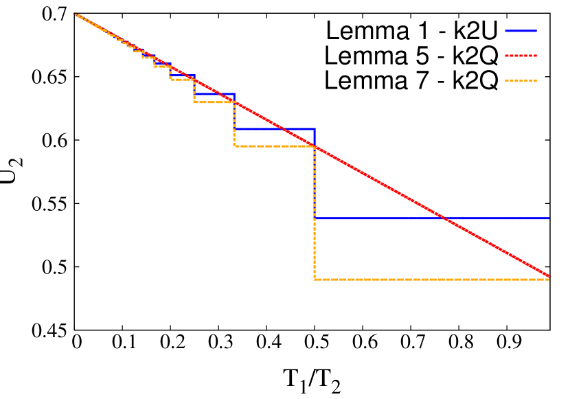
Figure 2: Adopting different tests from $\mathbf{k^{2}U}$ and $\mathbf{k^{2}Q}$ for RM uniprocessor scheduling with $k=2$.

5 Analysis for Sporadic Task Models

This section examines the applicability of the $\mathbf{k^{2}U}$ and $\mathbf{k^{2}Q}$ frameworks to derive utilization-based schedulability analysis and response-time analysis for sporadic task systems in uniprocessor systems. We will consider constrained-deadline systems in Section 5.1 and arbitrary-deadline systems in Section 5.2. For a specified fixed-priority scheduling algorithm, let $hp(\tau_{k})$ be the set of tasks with higher priority than $\tau_{k}$. We now classify the task set $hp(\tau_{k})$ into two subsets:

• $hp_{1}(\tau_{k})$ consists of the higher-priority tasks with periods smaller than $D_{k}$.

• $hp_{2}(\tau_{k})$ consists of the higher-priority tasks with periods larger than or equal to $D_{k}$.

For the rest of this section, we will implicitly assume $C_{k}>0$.

5.1 Constrained-Deadline

For a constrained-deadline task $\tau_{k}$, the schedulability test in Eq. (1) is equivalent to the verification of the existence of $0<t\leq D_{k}$ such that

$$C_{k}+\sum_{\tau_{i}\in hp_{2}(\tau_{k})}C_{i}+\sum_{\tau_{i}\in hp_{1}(\tau_{k})}\left\lceil{\frac{t}{T_{i}}}\right\rceil C_{i}\leq t.$$ (16)

We can then create a virtual sporadic task $\tau_{k}^{\prime}$ with execution time $C_{k}^{\prime}=C_{k}+\sum_{\tau_{i}\in hp_{2}(\tau_{k})}C_{i}$, relative deadline $D_{k}^{\prime}=D_{k}$, and period $T_{k}^{\prime}=D_{k}$. It is clear that the schedulability test to verify the schedulability of task $\tau_{k}^{\prime}$ under the interference of the higher-priority tasks $hp_{1}(\tau_{k})$ is the same as that of task $\tau_{k}$ under the interference of the higher-priority tasks $hp(\tau_{k})$. For notational brevity, suppose that there are $k^{*}-1$ tasks, indexed as $1,2,\ldots,k^{*}-1$, in $hp_{1}(\tau_{k})$.

Adopting $\mathbf{k^{2}U}$:           Setting $t_{i}=\left(\left\lceil{\frac{D_{k}}{T_{i}}}\right\rceil-1\right)T_{i}$ for every task $\tau_{i}$ in $hp_{1}(\tau_{k})$, and indexing the tasks in a non-decreasing order of $t_{i}$ lead to the satisfaction of Definition 1 with $\alpha_{i}=1$ and $0<\beta_{i}\leq 1$. Therefore, we can apply Lemmas 1 and 2 to obtain the following theorem.

Theorem 1.

Task $\tau_{k}$ in a sporadic task system with constrained deadlines is schedulable by the fixed-priority scheduling algorithm if

$$(\frac{C_{k}^{\prime}}{D_{k}}+1)\prod_{\tau_{j}\in hp_{1}(\tau_{k})}(U_{j}+1)\leq 2$$ (17)

or

$$\frac{C_{k}^{\prime}}{D_{k}}+\sum_{\tau_{j}\in hp_{1}(\tau_{k})}U_{j}\leq k^{*}(2^{\frac{1}{k^{*}}}-1).$$ (18)

Corollary 1.

Task $\tau_{k}$ in a sporadic task system with implicit deadlines is schedulable by the RM scheduling algorithm if Lemmas 2 and 3 holds by setting $\frac{C_{k}}{t_{k}}$ as $U_{k}$, $\alpha=1$, and $\beta=1$.

The above result in Corollary 1 leads to the utilization bound $\ln{2}$ (by using Lemma 2 with $\alpha=1$ and $\beta=1$) for RM scheduling, which is the same as the Liu and Layland bound $\ln{2}$ [23]. It also leads to the hyperbolic bound for RM scheduling by Bini and Buttazzo [6] when adopting Theorem 1 directly.

Adopting $\mathbf{k^{2}Q}$:           Setting $t_{i}=\left(\left\lceil{\frac{D_{k}}{T_{i}}}\right\rceil-1\right)T_{i}$ for every task $\tau_{i}$ in $hp_{1}(\tau_{k})$, and indexing the tasks in a non-decreasing order of $t_{i}$ leads to the satisfaction of Definition 3 with $\alpha_{i}=1$ and $\beta_{i}=1$. For such a case, the last release ordering is well-defined by the sorting of the tasks above. Therefore, we can use Lemma 5 to derive the following theorem.

Theorem 2.

Task $\tau_{k}$ in a sporadic task system with constrained deadlines is schedulable by the fixed-priority scheduling algorithm if $\sum_{i=1}^{k^{*}-1}\frac{C_{i}}{D_{k}}\leq 1$ and

$$\frac{C_{k}^{\prime}}{D_{k}}\leq 1-\sum_{i=1}^{k^{*}-1}U_{i}-\sum_{i=1}^{k^{*}-1}\frac{C_{i}}{D_{k}}+\frac{\sum_{i=1}^{k^{*}-1}U_{i}(\sum_{\ell=i}^{k^{*}-1}C_{\ell})}{D_{k}},$$ (19)

in which the $k^{*}-1$ higher priority tasks in $hp_{1}(\tau_{k})$ are indexed in a non-decreasing order of $\left(\left\lceil{\frac{D_{k}}{T_{i}}}\right\rceil-1\right)T_{i}$.

Corollary 2.

Task $\tau_{k}$ in a sporadic task system with implicit deadlines is schedulable by the RM scheduling algorithm if Lemmas 5, 7, 8, or 9 holds by setting $\frac{C_{k}}{t_{k}}$ as $U_{k}$, $\alpha=1$, and $\beta=1$.

The above result in Corollary 2 leads to the utilization bound $2-\sqrt{2}$ (by using Lemma 9 with $\alpha=1$ and $\beta=1$) for RM scheduling, which is worse than the existing Liu and Layland bound $\ln{2}$ [23].

Moreover, the above utilization bound $2-\sqrt{2}$ has been also provided by Abdelzaher et al. [1] for uniprocessor deadline-monotonic scheduling when an aperiodic task may generate different task instances (jobs) with different combinations of execution times and minimum inter-arrival times. Such a model is a more general model than the sporadic task model. Under such a setting, the $\mathbf{k^{2}U}$ framework cannot be used, whereas the $\mathbf{k^{2}Q}$ framework is very suitable.

5.2 Arbitrary-Deadline

The schedulability analysis for arbitrary-deadline sporadic task sets is to use a busy-window concept to evaluate the worst-case response time [20]. That is, we release all the higher-priority tasks together with task $\tau_{k}$ at time $0$ and all the subsequent jobs are released as early as possible by respecting to the minimum inter-arrival time. The busy window finishes when a job of task $\tau_{k}$ finishes before the next release of a job of task $\tau_{k}$. It has been shown in [20] that the worst-case response time of task $\tau_{k}$ can be found in one of the jobs of task $\tau_{k}$ in the busy window. For the $h$-th job of task $\tau_{k}$ in the busy window, let the finishing time $R_{k,h}$ is the minimum $t$ such that

$$hC_{k}+\sum_{i=1}^{k-1}\left\lceil{\frac{t}{T_{i}}}\right\rceil C_{i}\leq t,$$

and, hence, its response time is $R_{k,h}-(h-1)T_{k}$. The busy window of task $\tau_{k}$ finishes on the $h$-th job if $R_{k,h}\leq hT_{k}$.

A simpler sufficient schedulability test for a task $\tau_{k}$ is to test whether the length of the busy window is within $D_{k}$. If so, all invocations of task $\tau_{k}$ released in the busy window can finish before their relative deadline. Such an observation has also been adopted in [13]. Therefore, a sufficient test is to verify whether

$$\exists t\mbox{ with }0<t\leq D_{k}{\;\;and\;\;}\left\lceil{\frac{t}{T_{k}}}\right\rceil C_{k}+\sum_{\tau_{i}\in hp(\tau_{k})}\left\lceil{\frac{t}{T_{i}}}\right\rceil C_{i}\leq t.$$ (20)

If the condition in Eq. (20) holds, it implies that the busy window (when considering task $\tau_{k}$) is no more than $D_{k}$, and, hence, task $\tau_{k}$ has worst-case response time no more than $D_{k}$.

Similarly, we can use $hp_{1}(\tau_{k})$ and $hp_{2}(\tau_{k})$, as in Section 5.1, and, then create a virtual sporadic task $\tau_{k}^{\prime}$ with execution time $C_{k}^{\prime}=\left\lceil{\frac{D_{k}}{T_{k}}}\right\rceil C_{k}+\sum_{\tau_{i}\in hp_{2}(\tau_{k})}C_{i}$, relative deadline $D_{k}^{\prime}=D_{k}$, and period $T_{k}^{\prime}=D_{k}$. For notational brevity, suppose that there are $k^{*}-1$ tasks, indexed as $1,2,\ldots,k^{*}-1$, in $hp_{1}(\tau_{k})$.

Adopting $\mathbf{k^{2}U}$:           Setting $t_{i}=\left(\left\lceil{\frac{D_{k}}{T_{i}}}\right\rceil-1\right)T_{i}$, and indexing the tasks in a non-decreasing order of $t_{i}$ leads to the satisfaction of Definition 1 with $\alpha_{i}=1$ and $\beta_{i}\leq 1$. Therefore, we can apply Lemmas 1 and 2 to obtain the following theorem.

Theorem 3.

Task $\tau_{k}$ in a sporadic task system with arbitrary deadlines is schedulable by the fixed-priority scheduling algorithm if

$$(\frac{C_{k}^{\prime}}{D_{k}}+1)\prod_{\tau_{j}\in hp_{1}(\tau_{k})}(U_{j}+1)\leq 2$$ (21)

or

$$\frac{C_{k}^{\prime}}{D_{k}}+\sum_{\tau_{j}\in hp_{1}(\tau_{k})}U_{j}\leq k^{*}(2^{\frac{1}{k^{*}}}-1).$$ (22)

Adopting $\mathbf{k^{2}Q}$:           If we use the busy-window concept to analyze the schedulability of task $\tau_{i}$ by using Eq. (20), we can reach the following theorem directly by Lemma 5.

Theorem 4.

Task $\tau_{k}$ in a sporadic task system is schedulable by the fixed-priority scheduling algorithm if $\sum_{i=1}^{k^{*}-1}\frac{C_{i}}{D_{k}}\leq 1$ and

$$\frac{C_{k}^{\prime}}{D_{k}}\leq 1-\sum_{i=1}^{k^{*}-1}U_{i}-\sum_{i=1}^{k^{*}-1}\frac{C_{i}}{D_{k}}+\frac{\sum_{i=1}^{k^{*}-1}U_{i}(\sum_{\ell=i}^{k^{*}-1}C_{\ell})}{D_{k}},$$ (23)

in which $C_{k}^{\prime}=\left\lceil{\frac{D_{k}}{T_{k}}}\right\rceil C_{k}+\sum_{\tau_{i}\in hp_{2}(\tau_{k})}C_{i}$, and the $k^{*}-1$ higher priority tasks in $hp_{1}(\tau_{k})$ are indexed in a non-decreasing order of $\left(\left\lceil{\frac{D_{k}}{T_{i}}}\right\rceil-1\right)T_{i}$.

Analyzing the schedulability by using Theorem 4 can be good if $\frac{D_{k}}{T_{k}}$ is small. However, as the busy window may be stretched when $\frac{D_{k}}{T_{k}}$ is large, it may be too pessimistic. Suppose that $t_{j}=\left(\left\lceil{\frac{R_{k,h}}{T_{j}}}\right\rceil-1\right)T_{j}$ for a higher priority task $\tau_{j}$. We index the tasks such that the last release ordering $\pi$ of the $k-1$ higher priority tasks is with $t_{j}\leq t_{j+1}$ for $j=1,2,\ldots,k-2$. Therefore, we know that $R_{k,h}$ is upper bounded by finding the maximum

$$t_{k}=hC_{k}+\sum_{i=1}^{k-1}t_{i}U_{i}+\sum_{i=1}^{k-1}C_{i},$$ (24)

with $0\leq t_{1}\leq t_{2}\leq\cdots\leq t_{k-1}\leq t_{k}$ and

$$hC_{k}+\sum_{i=1}^{k-1}t_{i}U_{i}+\sum_{i=1}^{j-1}C_{i}>t_{j}, \forall j=1,2,\ldots,k-1.$$ (25)

Therefore, the above derivation of $R_{k,h}$ satisfies Definition 4 with $\alpha_{i}=1$, and $\beta_{i}=1$ for any higher priority task $\tau_{i}$. However, it should be noted that the last release time ordering $\pi$ is actually unknown since $R_{k,h}$ is unknown. Therefore, we have to apply Lemma 11 for such cases to obtain the worst-case ordering.

Lemma 12.

Suppose that $\sum_{i=1}^{k-1}U_{i}\leq 1$. Then, for any $h\geq 1$ and $C_{k}>0$, we have

$$R_{k,h}\leq\frac{hC_{k}+\sum_{i=1}^{k-1}C_{i}-\sum_{i=1}^{k-1}U_{i}(\sum_{\ell=i}^{k-1}C_{\ell})}{1-\sum_{i=1}^{k-1}U_{i}},$$ (26)

where the $k-1$ higher-priority tasks are ordered in a non-increasing order of their periods.

The worst-case response time for such cases can be set to $h=1$, in which the detailed proof is in [9, 12].

Theorem 5.

Suppose that $\sum_{i=1}^{k}U_{i}\leq 1$. The worst-case response time of task $\tau_{k}$ is at most

$$R_{k}\leq\frac{C_{k}+\sum_{i=1}^{k-1}C_{i}-\sum_{i=1}^{k-1}U_{i}(\sum_{\ell=i}^{k-1}C_{\ell})}{1-\sum_{i=1}^{k-1}U_{i}},$$ (27)

where the $k-1$ higher-priority tasks are ordered in a non-increasing order of their periods.

Corollary 3.

Task $\tau_{k}$ in a sporadic task system is schedulable by the fixed-priority scheduling algorithm if $\sum_{i=1}^{k}U_{i}\leq 1$ and

$$\frac{C_{k}}{D_{k}}\leq 1-\sum_{i=1}^{k-1}U_{i}-\frac{\sum_{i=1}^{k-1}C_{i}}{D_{k}}+\frac{\sum_{i=1}^{k-1}U_{i}(\sum_{\ell=i}^{k-1}C_{\ell})}{D_{k}},$$ (28)

where the $k-1$ higher-priority tasks are ordered in a non-increasing order of their periods.

5.3 Analytical Comparison of $\mathbf{k^{2}Q}$ and $\mathbf{k^{2}U}$

The utilization-based worst-case response-time analysis in Theorem 5 is analytically tighter than the best known result, $R_{k}\leq\frac{C_{k}+\sum_{i=1}^{k-1}C_{i}-\sum_{i=1}^{k-1}U_{i}C_{i}}{1-\sum_{i=1}^{k-1}U_{i}}$, by Bini et al. [7]. Lehoczky [20] also provides the total utilization bound of RM scheduling for arbitrary-deadline systems. The analysis in [20] is based on the Liu and Layland analysis [23]. The resulting utilization bound is a function of $\Delta=\max_{\tau_{i}}\{\frac{D_{i}}{T_{i}}\}$. When $\Delta$ is $1$, it is an implicit-deadline system. The utilization bound in [20] has a closed-form when $\Delta$ is an integer. However, calculating the utilization bound for non-integer $\Delta$ is done asymptotically for $k=\infty$ with complicated analysis. Bini [5] provides a total utilization bound of RM scheduling, based on the quadratic response time analysis in [7], that works for any arbitrary ratio of $\max_{\tau_{i}}\{\frac{D_{i}}{T_{i}}\}$.

For constrained-deadline sporadic task sets, since the same test in Eq. (16) is used for constructing Definition 1 and Definition 3, the result (with respect to the conditions in Theorem 1, Corollary 1, Theorem 5, and Corollary 2) by using $\mathbf{k^{2}U}$ is superior to that by using $\mathbf{k^{2}Q}$. The speedup factor of the test in Eq. (17) in Theorem 3 has been proved to be $1.76322$, which is also better than that in Eq. (19) in Theorem 4. However, the quadratic bound in Eq. (19) can be better than the hyperbolic bound in Eq. (17), as demonstrated in the evaluations.

For arbitrary-deadline sporadic task sets, two different tests are applied: one comes from Eq. (20) for constructing Theorem 3 and Theorem 4 and another comes from Eqs. (24) and (25) for construction Theorem 5 and Corollary 3. It should be clear that the test from Eqs. (24) and (25) is tighter than that from Eq. (20). Therefore, these results are not analytically comparable.

Note that we can also use Lemma 4 by defining the values of $\alpha_{i}$ and $\beta_{i}$ for each task $\tau_{i}$ in $hp_{1}(\tau_{k})$ precisely to make the hyperbolic bound in Eq. (17) and Eq. (21) more precisely. Their performance will be provided in the evaluation results.

5.4 Simulation Environment

The rest of this section presents our evaluation results for the above tests. We generated a set of sporadic tasks. The cardinality of the task set was $10$. The UUniFast-Discard method [14] was adopted to generate a set of utilization values with the given goal. We used the approach suggested by Davis et al. [15] to generate the task periods according to a uniform distribution in the range of the logarithm of the task periods (i.e., log-uniform distribution). The order of magnitude $p$ to control the period values between the largest and smallest periods is parameterized in evaluations, (e.g., $1-10ms$ for $p=1$, $1-100ms$ for $p=2$, etc.). We evaluate these tests in uniprocessor systems with $p\in[1,2,3]$. The priority ordering of the tasks is assigned according to deadline-monotonic (DM) scheduling. The execution time was set accordingly, i.e., $C_{i}=T_{i}U_{i}$.

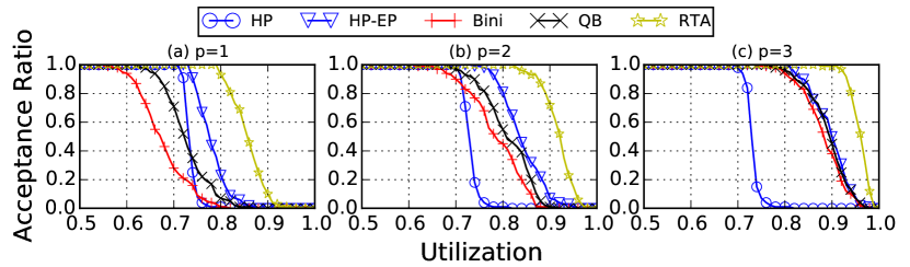
Figure 3: Performance evaluation on uniprocessor systems in terms of acceptance ratio for constrained-deadline uniprocessor systems where $\frac{D_{i}}{T_{i}}\in[0.8,1]$.

The metric to compare results is to measure the acceptance ratio of the above tests with respect to a given task set utilization. We generate 100 task sets for each utilization level. The acceptance ratio of a level is said to be the number of task sets that are schedulable under the schedulability test divided by the number of task sets for this level, i.e., 100.

5.5 Evaluation for Constrained Deadline Systems

Task relative deadlines were uniformly drawn from the interval $[0.8T_{i},T_{i}]$. The evaluated tests are as follows:

• RTA: the exact response time test by Lehoczky et al. [21].

• Bini: the linear-time response time bound by Bini et al. [7].

• HP (from $\mathbf{k^{2}U}$): Eq. (17) in Theorem 1 in this report.

• HP-EP (from $\mathbf{k^{2}U}$): using Lemma 4 (with a more precise extreme point) by defining the values of $\alpha_{i}$ and $\beta_{i}$ for each task $\tau_{i}$ in $hp_{1}(\tau_{k})$ precisely in this report. This improves HP.

• QB (from $\mathbf{k^{2}Q}$): Eq. (19) in Theorem 2 in this report.

Results. Figure 3 shows that the performance of the above tests in terms of acceptance ratios, for three different settings of $p$. The tests by HP-EP, Bini, QB, and RTA are sensitive to $p$: the larger the value of $p$ is, the more the test sets they admit. In the case of $p=1$, the test by Bini (the QB test, respectively) can admit all task sets with their total utilizations of up to $55\%$ ($60\%$, respectively), and its performance starts to decline at utilization $55\%$ ($60\%$, respectively). On the other hand, the tests by HP and HP-EP can fully accept a task set with around $15\%$ more utilizations, but acceptance ratio of HP drops sharply and becomes completely ineffective at utilization $76\%$.

In the case of $p=1$, we can also see that test HP derived from $\mathbf{k^{2}U}$ and test QB derived from $\mathbf{k^{2}Q}$ are incomparable. HP itself becomes pessimistic since we do not take the different values of $\alpha_{i}$ to have more precise tests, whereas HP-EP is more precise. In general, for uniprocessor constrained-deadline task systems, we can observe that HP-EP outperforms the other polynomial-time tests. Due to the analytical dominance, we also see that the QB test dominates the test by Bini.

5.6 Evaluation for Arbitrary-Deadline Systems

Task relative deadlines were uniformly drawn from the interval $[T_{i},2T_{i}]$. The tests evaluated are shown as follows:

• RTA: the exact response time test by Lehoczky[20].

• Bini: the linear-time response time bound by Bini et al. [7].

• HP-Busy (from $\mathbf{k^{2}U}$): Eq. (21) from Theorem 3 in this report

• HP-EP (from $\mathbf{k^{2}U}$): using Lemma 4 (with a more precise extreme point) by defining the values of $\alpha_{i}$ and $\beta_{i}$ for each task $\tau_{i}$ in $hp_{1}(\tau_{k})$ precisely in this report. This improves HP-Busy.

• QB-Busy (from $\mathbf{k^{2}Q}$): Eq. (23) in Theorem 4 in this report.

• QB-Response (from $\mathbf{k^{2}Q}$): Eq. (28) in Corollary 3 in this report.

Results. Figure 4 compares the performance on arbitrary-deadline uniprocessor system where $\frac{D_{i}}{T_{i}}\in[1,2]$. Analytically, we know that test by QB is superior to that by Bini, which is the best-known test for arbitrary-deadline uniprocessor systems. The results shown in Figure  4 also support such dominance.

In the case of $p=1$, the acceptance ratio by Bini decreases steadily from utilization $68\%$ to $95\%$. On the other hand, the number of task sets accepted by QB-Response starts to decrease at utilization $75\%$. Test QB-Response is able to admit more task tests from utilization $68\%$ to $85\%$, compared to test Bini. With utilization more $85\%$, Bini performs better than QB-Busy. In the other cases, Bini outperforms QB-Busy.

For arbitrary-deadline systems, since the test in Eq. (20) is too pessimistic by checking whether the busy-window length is no more than $D_{k}$, HP-Busy, HP-EP, and QB-Busy do not perform very well. In the above experimental results, the quadratic forms by using $\mathbf{k^{2}Q}$ are better than the hyperbolic forms by using $\mathbf{k^{2}U}$ in such cases. This is due to the fact that these two tests start from different pseudo-polynomial time tests.

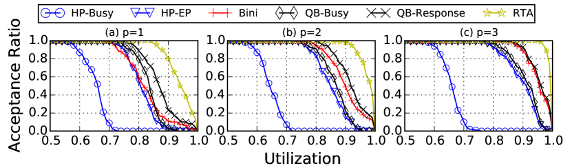
Figure 4: Performance evaluation on uniprocessor systems in terms of acceptance ratio for arbitrary-deadline uniprocessor systems where $\frac{D_{i}}{T_{i}}\in[1,2]$

6 Global RM Scheduling

This section demonstrates the two frameworks for multiprocessor global fixed-priority scheduling. We consider that the system has $M$ identical processors. For global fixed-priority scheduling, there is a global queue and a global scheduler to dispatch the jobs. We demonstrate the applicability for implicit-deadline sporadic systems under global RM.

Unfortunately, unlike uniprocessor systems, up to now, there is no exact schedulability test to verify whether task $\tau_{k}$ is schedulable by global RM. Therefore, existing schedulability tests (in pseudo-polynomial time or exponential time) are only sufficient tests. We will use three different tests for demonstrating the use of the $\mathbf{k^{2}U}$ and $\mathbf{k^{2}Q}$ frameworks and compare their results.

One way to quantify the quality of the resulting schedulability test is to use the capacity augmentation factor [22]. Suppose that the test is to verify whether the total utilization $\sum_{\tau_{i}}\frac{U_{i}}{M}\leq\frac{1}{b}$ and the maximum utilization $\max_{\tau_{i}}U_{i}\leq\frac{1}{b}$. Such a factor $b$ has been recently named as a capacity augmentation factor [22].

We only consider testing the schedulability of task $\tau_{k}$ under global RM, where $k>M$. For $k\leq M$, the global RM scheduling guarantees the schedulability of task $\tau_{k}$ if $U_{k}\leq 1$. Without loss of generality, we limit our presentation to the case that $T_{i}<T_{k}$ for $i=1,2,\ldots,k-1$, for the simplicity of presentation.

6.1 Adopted Pseudo-Polynomial-Time and Exponential-Time Tests

We now present three different tests that require pseudo-polynomial-time or exponential-time complexity.

Greedy-Carry-In: The first one is based on a simple observation to carry-in a job for each of the higher-priority tasks in the window of interest [16]. The following time-demand function $W_{i}(t)$ can be used for a simple sufficient schedulability test:

$$W_{i}(t)=\left(\left\lceil{\frac{t}{T_{i}}}\right\rceil-1\right)C_{i}+2C_{i}.$$ (29)

That is, we allow the first release of task $\tau_{i}$ to be inflated by a factor $2$, whereas the other jobs of task $\tau_{i}$ have the same execution time $C_{i}$. Therefore, task $\tau_{k}$ is schedulable under global RM on $M$ identical processors, if

$$\exists t\mbox{ with }0<t\leq T_{k}{\;\;and\;\;}C_{k}+\sum_{\tau_{i}\in hp(\tau_{k})}\frac{W_{i}(t)}{M}\leq t,$$ (30)

Bounded-Carry-In: The second test is based on the observation by Guan et al. [16] that we only have to consider $M-1$ tasks with carry-in jobs, for constrained-deadline task sets. For implicit-deadline task sets, this means that we only need to set $\alpha_{i}$ of some tasks to $\frac{2}{M}$, rather than all the $k-1$ tasks in Eq. (29). More precisely, we can define two different time-demand functions, depending on whether task $\tau_{i}$ is with a carry-in job or not:

$$W_{i}^{carry}(t)=\begin{cases}C_{i}&0<t<C_{i}\\ C_{i}+\left\lceil{\frac{t-C_{i}}{T_{i}}}\right\rceil C_{i}&otherwise,\end{cases}$$ (31)

and

$$W_{i}^{normal}(t)=\left\lceil{\frac{t}{T_{i}}}\right\rceil C_{i}.$$ (32)

Moreover, we can further over-approximate $W_{i}^{carry}(t)$, since $W_{i}^{carry}(t)\leq W_{i}^{normal}(t)+C_{i}$. Therefore, a sufficient schedulability test for testing task $\tau_{k}$ with $k>M$ for global RM is to verify whether

$$\exists 0<t\leq T_{k},C_{k}+\frac{(\sum_{\tau_{i}\in{\bf T}^{\prime}}C_{i})+(\sum_{i=1}^{k-1}W_{i}^{normal}(t))}{M}\leq t.$$ (33)

for all ${\bf T}^{\prime}\subseteq hp(\tau_{k})$ with $|{\bf T}^{\prime}|=M-1$. It is not necessary to enumerate all ${\bf T}^{\prime}$ with $|{\bf T}^{\prime}|=M-1$ if we can construct the task set ${\bf T}^{\prime}\subseteq hp(\tau_{k})$ with the maximum $\sum_{\tau_{i}\in{\bf T}^{\prime}}C_{i}$.

Forced-Forward: The third one is based on a reformulation of the forced-forward approach by Baruah et al. [3]. This is the reformulation in [9] based on a simple revision of the forced-forward algorithm in [3]. Let $U_{k}^{\max}$ be $\max_{j=1}^{k}\{U_{j}\}$. As shown and proved in [9], task $\tau_{k}$ in a sporadic task system with implicit deadlines is schedulable by a global RM on $M$ processors if

$$\forall y\geq 0,\forall 0\leq\omega_{i}\leq T_{i},\forall\tau_{i}\in hp(\tau_{k}),\exists t\mbox{ with }0<t\leq T_{k}+y{\;\;\;\;}$$

$$U_{k}^{\max}\cdot(T_{k}+y)+\frac{\sum_{i=1}^{k-1}\omega_{i}\cdot U_{i}+\left\lceil{\frac{t-\omega_{i}}{T_{i}}}\right\rceil C_{i}}{M}\leq t.$$ (34)

The schedulability condition in Eq. (34) requires to test all possible $y\geq 0$ and all possible settings of $0\leq\omega_{i}\leq T_{i}$ for the higher priority tasks $\tau_{i}$ with $i=1,2,\ldots,k-1$. Therefore, it needs exponential time (for all the possible combinations of $\omega_{i}$).

6.2 Polynomial-Time Tests by $\mathbf{k^{2}U}$

We now demonstrate how the $\mathbf{k^{2}U}$ framework can be adopted.

Based on Greedy-Carry-In: Such a case is pretty clear by setting $0<\alpha_{i}\leq\frac{2}{M}$ and $0<\beta_{i}\leq\frac{1}{M}$ in Definition 1 for task $\tau_{i}\in hp(\tau_{k})$. Therefore, by using Lemma 1 and Lemma 3, we have the following theorem.

Theorem 6.

Task $\tau_{k}$ in a sporadic implicit-deadline task system is schedulable by global RM on $M$ processors if

$$(\frac{C_{k}}{T_{k}}+2)\prod_{\tau_{i}\in hp(\tau_{k})}(\frac{U_{i}}{M}+1)\leq 3,$$ (35)

or

$$\sum_{\tau_{i}\in hp(\tau_{k})}\frac{U_{i}}{M}\leq\ln{\frac{3}{\frac{C_{k}}{T_{k}}+2}}.$$ (36)

Based on Bounded-Carry-In: There are two ways to use $\mathbf{k^{2}U}$. In the first case, we consider that $C_{i}$ for task $\tau_{i}$ in $hp(\tau_{k})$ is known. For such a case, we simply have to put the $M-1$ higher-priority tasks with the largest execution times into ${\bf T}^{\prime}$. This can be imagined as if we increase the execution time of task $\tau_{k}$ from $C_{k}$ to $C_{k}^{\prime}=C_{k}+\frac{\sum_{\tau_{i}\in{\bf T}^{\prime}}C_{i}}{M}$. Therefore, we still have $0<\alpha_{i}\leq\frac{1}{M}$ and $0<\beta_{i}\leq\frac{1}{M}$ for $\tau_{i}\in hp(\tau_{k})$. Therefore, by using Lemma 1 and Lemma 3, we have the following theorem:

Theorem 7.

Task $\tau_{k}$ in a sporadic implicit-deadline task system is schedulable by global RM on $M$ processors if

$$(\frac{C_{k}^{\prime}}{T_{k}}+1)\prod_{\tau_{i}\in hp(\tau_{k})}(\frac{U_{i}}{M}+1)\leq 2,$$ (37)

or

$$\sum_{\tau_{i}\in hp(\tau_{k})}\frac{U_{i}}{M}\leq\ln{\frac{2}{\frac{C_{k}^{\prime}}{T_{k}}+1}},$$ (38)

where $C_{k}^{\prime}=C_{k}+\frac{\sum_{\tau_{i}\in{\bf T}^{\prime}}C_{i}}{M}$.

In the second case, if only the task utilizations are given, we are not sure which tasks should be put into the carry-in task set ${\bf T}^{\prime}$. That is, if we are testing the worst-case period assignments of the higher-priority tasks in $hp(\tau_{k})$, we need to enumerate ${\bf T}^{\prime}$. Nevertheless, if ${\bf T}^{\prime}$ with $|{\bf T}^{\prime}|=M-1$ is specified, the translation to the $\mathbf{k^{2}U}$ framework is as follows: (1) the parameters are $0<\alpha_{i}\leq\frac{2}{M}$ and $0<\beta_{i}\leq\frac{1}{M}$ by using Eq. (33) if $\tau_{i}$ is in ${\bf T}^{\prime}$, and (2) the parameters are $\alpha_{i}=\frac{1}{M}$ and $0<\beta_{i}\leq\frac{1}{M}$ by using Eq. (33) if $\tau_{i}$ is not in ${\bf T}^{\prime}$. It may seem at first glance that we have to check all possible permutations of ${\bf T}^{\prime}$. Fortunately, with the analysis in [10, 11], the worst permutation of ${\bf T}^{\prime}$ is to the $M-1$ higher-priority tasks with the largest utilization into ${\bf T}^{\prime}$. This leads to the following theorem by extending Lemma 4.

Theorem 8.

Task $\tau_{k}$ in a sporadic implicit-deadline task system is schedulable by global RM on $M$ processors if

$$0<U_{k}\leq 1-\sum_{i=1}^{k-1}\frac{U_{i}(\alpha_{i}+\frac{1}{M})}{\prod_{j=i}^{k-1}(\frac{1}{M}U_{j}+1)},$$ (39)

by indexing the $k-1$ higher-priority tasks in a non-decreasing order of $U_{i}$ and assigning $\alpha_{1},\alpha_{2},\ldots,\alpha_{k-M}$ to $\frac{1}{M}$ and $\alpha_{k-M+1},\alpha_{k-M+2},\ldots,\alpha_{k-1}$ to $\frac{2}{M}$.

Based on Forced-Forward: Formulating the test in Eq. (34) into the $\mathbf{k^{2}U}$ framework is problematic. Suppose that $T_{k}$ is $1$. Assume that $y$ is set to $0$, $\omega_{i}$ is set to $0.1$, and $T_{i}$ is set to $0.92$. Under the above setting, $t_{i}$ is $0.1$, and $\alpha_{i}$ is $1$, $\beta_{i}$ is $9.2$. In fact, we even cannot safely set $\beta_{i}$ to any possible value except $\infty$ if $t_{i}$ is small enough. Therefore, constructing parameters based on Definition 1 is not possible (or non-trivial).

6.3 Polynomial-Time Tests by $\mathbf{k^{2}Q}$

Based on Greedy-Carry-In: This is possible by setting $0<\alpha_{i}\leq\frac{2}{M}$ and $0<\beta_{i}\leq\frac{1}{M}$ and applying Lemma 5. However, since the results are not superior to the one with bounded-carry-in, we omit it.

Based on Bounded-Carry-In: To use $\mathbf{k^{2}Q}$, we are certain about which tasks should be put into the carry-in task set ${\bf T}^{\prime}$ by assuming that $C_{i}$ and $T_{i}$ are both given. That is, we simply have to put the $M-1$ higher-priority tasks with the largest execution times into ${\bf T}^{\prime}$. This can be imagined as if we increase the execution time of task $\tau_{k}$ from $C_{k}$ to $C_{k}^{\prime}=C_{k}+\frac{\sum_{\tau_{i}\in{\bf T}^{\prime}}C_{i}}{M}$.

This leads to the following theorem by using Lemma 5.

Theorem 9.

Task $\tau_{k}$ in a sporadic implicit-deadline task system is schedulable by global RM on $M$ processors if $\sum_{i=1}^{k-1}C_{i}\leq MT_{k}$ and

$$\small U_{k}\leq 1-\frac{\sum_{\tau_{i}\in{\bf T}^{\prime}}C_{i}}{MT_{k}}-\sum_{i=1}^{k-1}\frac{U_{i}}{M}-\frac{\sum_{i=1}^{k-1}C_{i}}{MT_{k}}+\frac{\sum_{i=1}^{k-1}(U_{i}\sum_{\ell=i}^{k-1}C_{\ell})}{M^{2}T_{k}}.$$ (40)

by indexing the $k-1$ higher-priority tasks in a non-decreasing order of $(\left\lceil{\frac{T_{k}}{T_{i}}}\right\rceil-1)T_{i}$ and by putting the $M-1$ higher-priority tasks with the largest execution times into ${\bf T}^{\prime}$.

We can of course revise the statement in Theorem 9 by adopting Lemma 7 and Lemma 8 to construct schedulability tests by using only task utilizations.

Based on Forced-Forward: We present the corresponding polynomial-time schedulability tests for global fixed-priority scheduling. By using the forced-forward test, we can adopt the $\mathbf{k^{2}Q}$ framework by setting $\alpha_{i}=\frac{1}{M}$ and $\beta_{i}=\frac{1}{M}$. Due to the fact that $T_{i}\leq T_{k}$ for any task $\tau_{i}\in hp(\tau_{k})$, i.e., $C_{i}\leq U_{i}T_{k}$, under global RM, we can reach the following theorems and corollary, where the proofs are in [9].

Theorem 10.

Let $U_{k}^{\max}$ be $\max_{j=1}^{k}U_{j}$. Task $\tau_{k}$ in a sporadic task system with implicit deadlines is schedulable by global RM on $M$ processors if

$$U_{k}^{\max}\leq 1-\sum_{i=1}^{k-1}\frac{U_{i}}{M}-\frac{\sum_{i=1}^{k-1}C_{i}}{MT_{k}}+\frac{\sum_{i=1}^{k-1}U_{i}(\sum_{\ell=i}^{k-1}C_{\ell}))}{M^{2}T_{k}},$$ (41)

by ordering the $k-1$ higher-priority tasks in a non-increasing order of $T_{i}$.

Theorem 11.

Let $U_{k}^{\max}$ be $\max_{j=1}^{k}U_{j}$. Task $\tau_{k}$ in a sporadic task system with implicit deadlines is schedulable by global RM on $M$ processors if

$$U_{k}^{\max}\leq 1-\frac{2}{M}\sum_{i=1}^{k-1}U_{i}+\frac{0.5}{M^{2}}\left((\sum_{i=1}^{k-1}U_{i})^{2}+(\sum_{i=1}^{k-1}U_{i}^{2})\right)$$ (42)

or

$$\frac{\sum_{j=1}^{k-1}U_{j}}{M}\leq\left(\frac{k-1}{k}\right)\left(2-\sqrt{2+2U_{k}^{\max}\frac{k}{k-1}}\right).$$ (43)

Corollary 4.

The capacity augmentation factor of global RM for a sporadic system with implicit deadlines is $\frac{3+\sqrt{7}}{2}\approx 2.823$.

6.4 Analytical Comparison of $\mathbf{k^{2}Q}$ and $\mathbf{k^{2}U}$

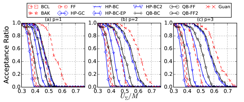
Figure 5: Acceptance ratio comparison on implicit-deadline 8 multiprocessor systems.

The utilization-based worst-case response-time analysis in Theorem 11 and Corollary 4 is analytically tighter than the best known result by Bertogna et al. [4] with linear-time tests. Moreover, our polynomial-time schedulability test extended to handle deadline-monotonic scheduling for constrained-deadline task sets based on the forced-forward analysis in [9] has the same speedup factor as the best known result in pseudo-polynomial time by Baruah et al. [3].

With respect to the capacity augmentation factors, the test derived from $\mathbf{k^{2}Q}$ by using the forced-forward approach obtains the best one, whereas the tests from bounded carry-in are worse. As shown in the above examples, different schedulability tests may lead to different quality of the schedulability tests. Therefore, these results are not analytically comparable. We will have to compare these results in the evaluations.

6.5 Evaluation Results

In this section, we conduct experiments using synthesized task sets for evaluating the proposed tests on multiprocessor systems. We first generated a set of sporadic tasks. The cardinality of the task set was $5$ times the number of processors, e.g., 40 tasks on 8 multiprocessor systems. The task sets were generated in a similar manner in Section 5.4. Tasks’ relative deadlines were equal to their periods.

The evaluated tests are as follows:

• BCL: the linear-time test in Theorem 4 in [4].

• FF: the pseudo-polynomial-time force-forward (FF) analysis in Eq. (5) in [3].

• BAK: the $O(n^{3})$ test in Theorem 11 in [2].

• Guan: the pseudo-polynomial-time response time analysis[16].

• HP-GC (from $\mathbf{k^{2}U}$): Eq. (35) from Theorem 6 based on greedy carry-in (GC) in this report.

• HP-BC (from $\mathbf{k^{2}U}$): Eq. (37) from Theorem 7 based on bounded carry-in (BC) in this report.

• HP-BC-EP (from $\mathbf{k^{2}U}$): using Lemma 4 (with a more precise extreme point) by defining the values of $\alpha_{i}$ and $\beta_{i}$ for each task $\tau_{i}$ in $hp(\tau_{k})$ precisely in this report. This improves HP-BC from Theorem 7 based on bounded carry-in (BC) in this report.

• HP-BC2 (from $\mathbf{k^{2}U}$): Eq. (39) from Theorem 8 based on bounded carry-in (BC) in this report.

• QB-BC (from $\mathbf{k^{2}Q}$): Eq. (40) in Theorem 9 based on bounded carryin (BC) in this report.

• QB-FF (from $\mathbf{k^{2}Q}$): Eq. (41) from Theorem 10 based on force-forward (FF) in this report.

• QB-FF2 (from $\mathbf{k^{2}Q}$): Eq. (42) from Theorem 11 based on force-forward (FF) in this report.

Among the above tests, BCL, HP-GC, HP-BC2, QB-FF and QB-FF2 can be implemented in linear time. Our other tests (HB-BC, HP-BC-EP, QB-BC) require to sort the higher-priority tasks to define the proper last release ordering; therefore, their time complexity is $O(n^{2}\log n)$ for a task set with $n$ tasks.

Results. Figure 5 depicts the result of the performance comparison. In all the cases, we can see that QB-BC and HP-BC-EP are superior to almost all the other polynomial-time tests. It may seem that QB-FF is superior to QB-BC when we inspect their schedulability tests. However, the way how we formulated the force-forward algorithm in Eq. (34) is also pessimistic by introducing $U_{k}^{\max}$ instead of just $U_{k}$. Such inflation from $U_{k}$ to $U_{k}^{\max}$ makes the analysis for the worst-case capacity-augmentation factor tighter, but also makes QB-FF with less acceptance ratio when testing tasks with utilization larger than the threshold $\frac{1}{2.84306}$. Therefore, if $U_{k}^{\max}>U_{k}+\sum_{\tau_{i}\in{\bf T}^{\prime}}\frac{C_{i}}{MT_{k}}$, then QB-FF is worse than QB-BC.

The greedy carry-in in HP-GC makes it too pessimistic. However, HP-BC is comparable with BAK. Among the linear-time tests, QB-FF outperforms the others in all the cases. Among the above tests, it is difficult to compare QB-BC and HP-BC-EP, since they perform very closely. Overall, most of the tests derived by using the two frameworks perform very well with low time complexity.

7 Conclusion

This report presents the similarly, difference, and the characteristics of the $\mathbf{k^{2}U}$ and $\mathbf{k^{2}Q}$ frameworks. These two frameworks have great potential to be used for deriving polynomial-time schedulability tests almost automatically, as soon as the corresponding parameters in Definitions 1, 3, and 4 can be constructed. In the past, exponential-time schedulability tests were typically not recommended and most of time ignored, as this requires very high complexity. However, by adopting these two frameworks, we have successfully shown that exponential-time schedulability tests may lead to good polynomial-time tests by using the $\mathbf{k^{2}U}$ and $\mathbf{k^{2}Q}$ frameworks. Both frameworks are needed and have to be applied for different cases. With these two frameworks, some difficult schedulability test and response time analysis problems may be solved by building a good (or exact) exponential-time test and applying these two frameworks.

These two frameworks are both useful and needed for different cases and applications. We have demonstrated their differences in details and present evaluation results for the schedulability tests derived from these two frameworks. For some cases, $\mathbf{k^{2}U}$ is better, and for some cases, $\mathbf{k^{2}Q}$ is better.

Acknowledgement: This paper has been supported by DFG, as part of the Collaborative Research Center SFB876 (http://sfb876.tu-dortmund.de/), and the priority program ”Dependable Embedded Systems” (SPP 1500 - http://spp1500.itec.kit.edu).

References

- [1] T. F. Abdelzaher, V. Sharma, and C. Lu. A utilization bound for aperiodic tasks and priority driven scheduling. IEEE Trans. Computers, 53(3):334–350, 2004.
- [2] T. P. Baker. An analysis of fixed-priority schedulability on a multiprocessor. Real-Time Systems, 32(1-2):49–71, 2006.
- [3] S. K. Baruah, V. Bonifaci, A. Marchetti-Spaccamela, and S. Stiller. Improved multiprocessor global schedulability analysis. Real-Time Systems, 46(1):3–24, 2010.
- [4] M. Bertogna, M. Cirinei, and G. Lipari. New schedulability tests for real-time task sets scheduled by deadline monotonic on multiprocessors. In Principles of Distributed Systems, pages 306–321. Springer, 2006.
- [5] E. Bini. The quadratic utilization upper bound for arbitrary deadline real-time tasks. IEEE Trans. Computers, 64(2):593–599, 2015.
- [6] E. Bini, G. C. Buttazzo, and G. M. Buttazzo. Rate monotonic analysis: the hyperbolic bound. Computers, IEEE Transactions on, 52(7):933–942, 2003.
- [7] E. Bini, T. H. C. Nguyen, P. Richard, and S. K. Baruah. A response-time bound in fixed-priority scheduling with arbitrary deadlines. IEEE Transactions on Computers, 58(2):279, 2009.
- [8] A. Burchard, J. Liebeherr, Y. Oh, and S. H. Son. New strategies for assigning real-time tasks to multiprocessor systems. pages 1429–1442, 1995.
- [9] J.-J. Chen, W.-H. Huang, and C. Liu. : A quadratic-form response time and schedulability analysis framework for utilization-based analysis. Computing Research Repository (CoRR), abs/1505.03883, 2015. extended report of the paper in RTSS 2016.
- [10] J.-J. Chen, W.-H. Huang, and C. Liu. : A general framework from k-point effective schedulability analysis to utilization-based tests. Computing Research Repository (CoRR), abs/1501.07084, 2015. extended report of the paper in RTSS 2015.
- [11] J.-J. Chen, W.-H. Huang, and C. Liu. k2U: A general framework from k-point effective schedulability analysis to utilization-based tests. In Real-Time Systems Symposium, RTSS, pages 107–118, 2015.
- [12] J.-J. Chen, W.-H. Huang, and C. Liu. k2Q: A quadratic-form response time and schedulability analysis framework for utilization-based analysis. In Real-Time Systems Symposium, RTSS, 2016.
- [13] R. Davis, T. Rothvoß, S. Baruah, and A. Burns. Quantifying the sub-optimality of uniprocessor fixed priority pre-emptive scheduling for sporadic tasksets with arbitrary deadlines. In Real-Time and Network Systems (RTNS), pages 23–31, 2009.
- [14] R. I. Davis and A. Burns. Improved priority assignment for global fixed priority pre-emptive scheduling in multiprocessor real-time systems. Real-Time Systems, 47(1):1–40, 2011.
- [15] R. I. Davis, A. Zabos, and A. Burns. Efficient exact schedulability tests for fixed priority real-time systems. Computers, IEEE Transactions on, 57(9):1261–1276, 2008.
- [16] N. Guan, M. Stigge, W. Yi, and G. Yu. New response time bounds for fixed priority multiprocessor scheduling. In IEEE Real-Time Systems Symposium, pages 387–397, 2009.
- [17] C.-C. Han and H. ying Tyan. A better polynomial-time schedulability test for real-time fixed-priority scheduling algorithms. In Real-Time Systems Symposium (RTSS), pages 36–45, 1997.
- [18] T.-W. Kuo, L.-P. Chang, Y.-H. Liu, and K.-J. Lin. Efficient online schedulability tests for real-time systems. Software Engineering, IEEE Transactions on, 29(8):734–751, 2003.
- [19] C.-G. Lee, L. Sha, and A. Peddi. Enhanced utilization bounds for qos management. IEEE Trans. Computers, 53(2):187–200, 2004.
- [20] J. P. Lehoczky. Fixed priority scheduling of periodic task sets with arbitrary deadlines. In RTSS, pages 201–209, 1990.
- [21] J. P. Lehoczky, L. Sha, and Y. Ding. The rate monotonic scheduling algorithm: Exact characterization and average case behavior. In IEEE Real-Time Systems Symposium, pages 166–171, 1989.
- [22] J. Li, J. Chen, K. Agrawal, C. Lu, C. Gill, and A. Saifullah. Analysis of federated and global scheduling for parallel real-time tasks. In Euromicro Conference on Real-Time Systems, 2014.
- [23] C. L. Liu and J. W. Layland. Scheduling algorithms for multiprogramming in a hard-real-time environment. Journal of the ACM (JACM), 20(1):46–61, 1973.
- [24] J. Wu, J. Liu, and W. Zhao. On schedulability bounds of static priority schedulers. In Real-Time and Embedded Technology and Applications Symposium (RTAS), pages 529–540, 2005.