Abstract

We study the problem of remote one-qubit mixed state creation using a pure initial state of two-qubit sender and spin-1/2 chain as a connecting line. We express the parameters of creatable states in terms of transition amplitudes. We show that the creation of complete receiver’s state-space can be achieved only in the chain engineered for the one-qubit perfect state transfer (PST) (for instance, in the fully engineered Ekert chain), the chain can be arbitrarily long in this case. As for the homogeneous chain, the creatable receiver’s state region decreases quickly with the chain length. Both homogeneous chains and chains engineered for PST can be used for the purpose of selective state creation, when only the restricted part of the whole receiver’s state space is of interest. Among the parameters of the receiver’s state, the eigenvalue is the most hard creatable one and therefore deserves the special study. Regarding the homogeneous spin chain, an arbitrary eigenvalue can be created only if the chain is of no more than 34 nodes. Alternating chain allows us to increase this length up to 68 nodes.

I Introduction

The problem of remote creation of a particular quantum state is one of fundamental problems in quantum communication. Its prototype is the pure quntum state transfer problem, which was first formulated in well-known paper by Bose Bose for the homogeneous ferromagnet spin chain with isotropic Heisenberg interaction. Now the state transfer represents a special direction in quantum information processing. Among the spin systems engineered for the either perfect or high-fidelity (probability) one-qubit pure state transfer, we mention such well-known systems as the spin chains with properly adjusted coupling constants (or the fully engineered spin chains) CDEL ; ACDE ; KS and the homogeneous chains with remote end nodes (the boundary-controlled GKMT ; WLKGGB and optimized boundary-controlled NJ ; SAOZ spin chains). In addition, the experimental realization of the perfect state transfer through the three-qubit chain in trichloroethylene is proposed in ZLZDLL .

Studing the perfect state transfer (PST) problem in spin chains shows its sensitivity to the chain parameters. Moreover, been achieved for a model system (such as the nearest neighbor XY Hamiltonian in CDEL ; ACDE ; KS ), it becomes destroyed by imperfections, such as remote node interactions and quantum noise, which always reduce the state transfer fidelity CRMF ; ZASO ; ZASO2 ; ZASO3 ; SAOZ so that the original state can not be perfectly transfered between the ends of a chain. As a consequence, the high-fidelity/probability state transfer becomes more popular in comparison with the PST, which is justified in numerous papers concerning different aspects of this subject, such as the entanglement Wootters ; HW ; P ; AFOV ; HHHH transfer through a quantum chain DFZ ; DZ ; BACVV2010 ; BACVV2011 ; LS , the entanglement creation between distant qubits BBVB ; BZ , the so-called ballistic quantum state transfer Banchi , the high-dimensional state transfer YGQ ; YGQ2 , the robustness of state transfer CRMF ; ZASO ; ZASO2 ; ZASO3 ; QWZ .

Nevertheless, the search for alternative ways of quantum communications free of the destructive effect of imperfections becomes more and more attractive. Thus, the so-called information transfer was proposed in Z_2012 . In this case we take care of transfer of all the state’s parameters (instead of the quantum state itself) from the sender to the receiver. These parameters appear linearly in the receiver’s state, so that we have to solve a system of linear algebraic equations to obtain these parameters on the receiver’s side. In turn, this requires non-quantum mechanical tool, which is a price for the robustnesses of the information transfer. The conclusion about robustness is based on a simple observation that any imperfection of the model changes the coefficients in the above linear system without changing the transferred parameters (as for the noise, also the averaged effect leads to such change of coefficients). Consequently, unlike the state transfer, this process is not sensitive to the parameters of the spin chain as well as to the imperfections of the experimental realization of the proposed model (nearest neighbor XY Hamiltonian was used in Z_2012 ).

In recent paper Z_2014 , the principles of both perfect state transfer Bose ; CDEL ; ACDE ; KS ; KF ; KZ_2008 ; GKMT ; FZ ; WLKGGB and state-information transfer Z_2012 were realized in the mixed state creation algorithm using short homogeneous spin-1/2 chains with nearest neighbor XY-interactions. The basic idea of that paper is to handle the parameters of the creatable state of the remote subsystem (receiver) varying the parameters of another subsystem (sender) through the local unitary transformations of the latter. Notice, that the most of earlier experiments realizing the remote state creation use photons as carriers of quantum information ZZHE ; BPMEWZ ; BBMHP ; PBGWK2 ; PBGWK ; DLMRKBPVZBW ; XLYG . State creation based on spin-1/2 chains is suitable for the state/information transfer/creation over the relatively short distances, for instance, inside of a particular quantum device.

In this paper we represent the detailed study of the remote one-qubit mixed state creation of the receiver (the last node of a chain) through the long spin-1/2 chain with a pure initial state of (at most) two-qubit sender (the first and the second nodes of a chain). We call the parameters varying with the purpose to create the needed receiver’s state as the control parameters, while the parameters of the receiver’s state are referred to as the creatable parameters. In the case of one-qubit sender, the time is required as one of the control parameters needed to create a large region of the receiver state-space. Therefore, this case can not be considered as the completely local control (i.e., the control through the local parameters of the sender’s initial state) of state-creation, because the required time instant must be reported to the receiver’s side (perhaps, through a classical communication channel). We concentrate on the completely local control achievable using the two-qubit sender (similar to ref.Z_2014 ). In this case the large creatable region can be covered at a properly fixed time instant just varying the parameters of the sender’s initial state. In other words, the time is not included in the list of control parameters. For a pure initial sender’s state, we express the parameters of creatable state in terms of the transition amplitudes and control parameters, so that the receiver’s density matrix acquires the very simple form. We show that the creation of the complete one-qubit receiver’s state-space can be achieved in the chain engineered for the one-qubit PST CDEL ; ACDE ; KS . The chain can be arbitrarily long in this case. As for the homogeneous chains, on the contrary, the creatable region decreases very quickly with an increase in the chain length. Apparently, this is an essential disadvantage of homogeneous chains. However we show that this disadvantage leads to some privileges of such chains in application to the problem of selective-region state creation, when we intend to work with a particular subregion of the receiver’s state space. Namely, the homogeneous chains reduce (or even completely remove) the possibility of a ”parasitic” state creation outside of the required subregion, if only this subregion is properly selected. Such selective state creation can be considered as the first step in construction of the ”branched” communication systems having several senders and one common receiver. Notice, that the chains engineered for the PST do not possess this property, although they can be used in the selective-region state creation as well.

Following ref.Z_2014 , by the state of the receiver $B$ we mean the reduced density matrix (the marginal matrix)

$$\rho^{B}=Tr_{rest}\rho,$$ (1)

where $\rho$ is the density matrix of the whole system and the trace is calculated over the all nodes except for the last one (receiver’s node). The one-qubit receiver’s state space is parametrized by three parameters. One of them is the eigenvalue and two others are associated with the eigenvectors. In turn, among two latter parameters, there is the phase which has no restriction for creation Z_2014 , i.e., any required value of this phase can be created by a proper choice of the control parameters. Another eigenvector parameter can, in principle, be tuned to the required value by the local unitary transformation of the receiver. On the contrary, the eigenvalue represents the most hard creatable parameter because it is effected by the evolution and it is not sensitive to the local unitary transformations of the receiver. Thus the eigenvalue creation deserves a special attention. It turns out that any eigenvalue can be created in the homogeneous chain of no more than $N_{c}=34$ nodes. Of cause, any value of this parameter can be created in the fully engineered chains of arbitrary length, but such chains themselves are hard for the practical realization. Alternatively, we consider the alternating chain with even number of nodes for the purpose of remote eigenvalue creation and show that this chain increases the parameter $N_{c}$ up to 68 nodes.

Finally we shall mention that the teleportation BBCJPW ; BPMEWZ ; BBMHP can be considered as a prototype of the remote state creation. Teleportation is aimed on the long distance transfer of an unknown state using the entangled pairs of bits YS1 ; YS2 ; ZZHE . An inherent feature of teleportation is that it requires the classical channel of information transfer as a necessary component of the teleportation protocol, unlike the state transfer/creation problem. Set of modifications of the state teleportation/creation protocol can be found in BDSSBW ; BHLSW ; XLYG ; G .

The structure of this paper is following. In Sec.II, we represent the basic analytical results concerning the map between the control parameters of sender’s initial state and the creatable parameters of the receiver’s state. We show, in particular, that the creatable region covers the whole receiver’s state-space at the time instant of PST. The state creation in chains governed by the nearest neighbor XY Hamiltonian is studied in more details in the same section. In Sec.III, we study the state creation inside of the selected subregions of the receiver’s state space on the basis of homogeneous and fully engineered Ekert chains. Sec.IV is devoted to the eigenvalue creation in the long homogeneous and alternating chains, as well as in the chains engineered for the PST. The basic results of paper are collected in Sec.V.

II One-qubit receiver’s state creation through pure two-qubit initial sender’s state

II.1 One-excitation evolution

In this section we introduce two requirements simplifying the spin dynamics calculation.

1. The Hamiltonian $H$ commutes with the $z$-projection of the total spin momentum:

   $$[H,I_{z}]=0.$$ (2)

2. The initial state is a superposition of the pure states with up to single excited spin.

These two requirements allow us to consider the dynamics in the following basis of $N+1$ independent vectors (instead of $2^{N}$ independent vectors in general case of $N$-qubit dynamics):

$$|0\rangle\equiv|\underbrace{0\dots 0}_{N}\rangle,\;\;\;|n\rangle\equiv|\underbrace{0\dots 0}_{n-1}1\underbrace{0\dots 0}_{N-n}\rangle,\;\;n=1,\dots,N.$$ (3)

Next, we can write the Hamiltonian in the following two-block diagonal form

$$H={\mbox{diag}}(H_{0},H_{1}),$$ (4)

where $H_{0}$, is written in the basis of a single vector $|0\rangle$ (thus, it is a scalar) and the block $H_{1}$ is written in the basis $|n\rangle$, $n=1,\dots,N$. Without the loss of generality, we take $H_{0}=0$.

Let us consider a pure initial state $|\Psi_{0}\rangle$ of our quantum system. In accordance with the Schrödinger equation, evolution of this state reads:

$$|\Psi(t)\rangle=e^{-iHt}|\Psi_{0}\rangle.$$ (5)

As known, the receiver’s state is mixed in general and can be written as (in the case of one-excitation)

$$\rho^{B}\equiv{\mbox{Tr}}_{1,2,\dots,N-1}\rho=\left(\begin{array}[]{cc}1-|f_{N}|^{2}&f_{N}^{*}f_{0}\cr f_{N}f_{0}^{*}&|f_{N}|^{2}\end{array}\right)=\left(\begin{array}[]{cc}1-R_{N}^{2}&R_{N}R_{0}e^{-2\pi i(\Phi_{N}-\Phi_{0})}\cr R_{N}R_{0}e^{2\pi i(\Phi_{N}-\Phi_{0})}&R_{N}^{2}\end{array}\right).$$ (10)

Here the trace is taken over the nodes $1,\dots,N-1$, star means the complex conjugate value and $f_{N}$, $f_{0}$ are the probability amplitudes,

$$f_{i} = \langle i|e^{-iHt}|\Psi_{0}\rangle=R_{i}e^{2\pi i\Phi_{i}},\;\;i=0,\dots,N,$$ (11)

where $R_{i}$ and $\Phi_{i}$ are real parameters and $R_{i}$ are positive. Remember a natural constraint

$$|f_{N}|^{2}+|f_{0}|^{2}\leq 1\;\;\Rightarrow\;\;R_{N}^{2}+R_{0}^{2}\leq 1,$$ (12)

where the equality corresponds to the pure state creation because in this case $f_{i}\equiv 0$ ($i\neq 0,N$) and the only nonzero eigenvalue equals one (the last statement can be directly verified using eq.(25) derived below). This phenomenon is equivalent to the PST in the case of one-qubit sender. Constraint (12) suggests the following parametrization of $R_{N}$:

$$R_{N}=\sqrt{1-R_{0}^{2}}R,$$ (13)

therewith

$$0\leq R_{0}\leq 1,\;\;$$ (14)

$$0\leq R\leq 1,$$ (15)

$$0\leq\Phi\leq 1,\;\;\Phi=\Phi_{N}-\Phi_{0}.$$ (16)

Thus, three parameters $R_{0}$, $R$ and $\Phi$ (which are defined by the initial state of our quantum system and by the interaction Hamiltonian) completely characterize the possible creatable receiver’s state. However, representation (10) of the density matrix $\rho^{B}$ is not a preferred one because it does not give us a simple way to estimate whether the whole state space of the receiver is creatable. The following factorized representation allows us to realize this estimation giving the convenient parametrization of the receiver’s state-space:

$$\rho^{B}=U^{B}\Lambda^{B}(U^{B})^{+},$$ (17)

where $\Lambda^{B}$ is the diagonal matrix of eigenvalues and $U^{B}$ is the matrix of eigenvectors, which read as follows in our case:

$$\Lambda^{B}={\mbox{diag}}(\lambda,1-\lambda),$$ (18)

$$U^{B}=\left(\begin{array}[]{cc}\cos\frac{\beta_{1}\pi}{2}&-e^{-2i\beta_{2}\pi}\sin\frac{\beta_{1}\pi}{2}\cr e^{2i\beta_{2}\pi}\sin\frac{\beta_{1}\pi}{2}&\cos\frac{\beta_{1}\pi}{2}.\end{array}\right)$$ (21)

with $\lambda$ and $\beta_{i}$ ($i=1,2$) varying inside of the intervals

$$\frac{1}{2}\leq\lambda\leq 1,$$ (22)

$$0\leq\beta_{i}\leq 1,\;\;i=1,2.$$ (23)

Intervals (22) and (23) cover the whole state-space of the receiver. Note that the maximally mixed state is characterized by a single parameter $\lambda=\frac{1}{2}$.

Another advantage of representation (17) is that it separates the whole parameter space of receiver’s state into two parts:

$${\mbox{The independent eigenvalues of $\rho^{B}$: the only parameter $\lambda$}},$$ (24)

$${\mbox{The independent eigenvector-parameters of $\rho^{B}$: $\beta_{1}$ and $\beta_{2}$ }}.$$

Obviously, the parameters $\lambda$ and $\beta_{i}$, $i=1,2$, are related with $R_{0}$, $R$ and $\Phi$ as follows:

$$\lambda = \frac{1}{2}\left(1+\sqrt{(1-2R_{N}^{2})^{2}+4R_{N}^{2}R_{0}^{2}}\right),$$ (25)

$$\cos\beta_{1}\pi = \frac{1-2R_{N}^{2}}{\sqrt{(1-2R_{N}^{2})^{2}+4R_{N}^{2}R_{0}^{2}}},\;\;\Rightarrow$$ (26)

$$\beta_{1}\pi = \arccos\frac{1-2R_{N}^{2}}{\sqrt{(1-2R_{N}^{2})^{2}+4R_{N}^{2}R_{0}^{2}}},$$ (27)

$$\beta_{2} = \Phi$$ (28)

with $R_{N}$ from (13). Clearly, if the triple $(R_{0},R,\Phi)$ can run all points in cube (14-16), then the triple $(\lambda,\beta_{1},\beta_{2})$ takes all values inside of the cube (22,23), and thus the whole receiver’s state-space is creatable. However, this is possible only in special cases (like Ekert chain in Sec.II.5). Usually, only a part of the receiver’s state-space can be created (see homogeneous chains in Sec.II.5). Formulas (25-28) represent the map between the control parameters of the sender (embedded in $R_{0}$, $R$ and $\Phi$) and the creatable parameters $\lambda$, $\beta_{1}$ and $\beta_{2}$ of the receiver. Now we specify the dependence on the control parameters introducing a particular sender’s initial state.

II.2 Two-node sender with one excitation initial state

For the purpose of effective remote control of the one-qubit receiver’s state, we take the two node sender with the pure one-excitation initial state of the following general form:

$$|\Psi_{0}^{S}\rangle=a_{0}|00\rangle+a_{1}|10\rangle+a_{2}|01\rangle,$$ (29)

$$\sum_{i=0}^{2}|a_{i}|^{2}=1,$$ (30)

where $a_{i}$ ($i=0,1,2$) are the control parameters with constraint (30). Since the common phase of a pure state does not effect the density matrix, we take the real positive $a_{0}$ without the loss of generality. Obviously, the above sender’s initial state can be obtained from the ground sender’s state $|00\rangle$ using the following $SU(3)$-transformation Z_2014 :

$$U^{A}=\left(\begin{array}[]{ccc}a_{0}&\displaystyle-\frac{a_{1}^{*}}{\sqrt{1-|a_{2}|^{2}}}&\displaystyle-\frac{a_{0}a_{2}^{*}}{\sqrt{1-|a_{2}|^{2}}}\cr a_{1}&\displaystyle\frac{a_{0}}{\sqrt{1-|a_{2}|^{2}}}&\displaystyle-\frac{a_{1}a_{2}^{*}}{\sqrt{1-|a_{2}|^{2}}}\cr a_{2}&0&\displaystyle\sqrt{1-|a_{2}|^{2}}\end{array}\right),\;\;\sum_{i=0}^{2}|a_{i}|^{2}=1,$$ (34)

i.e., $|\Psi_{0}^{S}\rangle=U^{A}|00\rangle$. This is a 5-parameter transformation (one real parameter $a_{0}$, two independent amplitudes and two phases of $a_{1}$ and $a_{2}$) and it represents a particular case of the general eight-parameter $SU(3)$ transformation. We will show that transformation (34) establishes the maximal possible control of the one-qubit receiver state in the framework of our model. Therewith the rest of the quantum system is in the ground initial state,

$$|\Psi_{0}^{rest}\rangle=|\underbrace{0,\dots,0}_{N-2}\rangle.$$ (35)

Thus, the initial state of the whole system reads:

$$|\Psi_{0}\rangle\equiv|\Psi_{0}^{S}\rangle\otimes|\Psi_{0}^{rest}\rangle=\sum_{i=0}^{2}a_{i}|i\rangle.$$ (36)

We see that the control capability of the sender can be described in two equivalent ways: by the parameters of initial state (see eq.(29)) and by the parameters of unitary transformation (34) of the ground sender’s state. Since the initial state itself seems to be more physical and more practical in comparison with the unitary transformation, hereafter we focus on formula (29).

Obviously, the control parameters appear linearly in evolution (5) of the state:

$$|\Psi(t)\rangle = e^{-iHt}|\Psi_{0}\rangle=a_{0}e^{-iH_{0}t}|0\rangle+\sum_{j=1}^{2}a_{j}e^{-iH_{1}t}|j\rangle=$$

$$a_{0}|0\rangle+\sum_{j=1}^{2}a_{j}e^{-iH_{1}t}|j\rangle.$$

Consequently, the probability amplitudes appearing in the receiver’s state (10) are also linear functions of the control parameters:

$$f_{N}(t) = \langle N|e^{-iHt}|\Psi_{0}\rangle=\sum_{j=1}^{2}a_{j}\langle N|e^{-iH_{1}t}|j\rangle=\sum_{j=1}^{2}a_{j}p_{Nj}(t),$$ (38)

$$f_{0}(t) = \langle 0|e^{-iHt}|\Psi_{0}\rangle=a_{0}\equiv R_{0},$$ (39)

where

$$p_{kj}(t)=\langle k|e^{-iH_{1}t}|j\rangle=r_{kj}(t)e^{2\pi i\chi_{kj}(t)},\;\;k,j>0,$$ (40)

$r_{kj}$ are positive amplitudes and $2\pi\chi_{kj}$ ($0\leq\chi_{kj}\leq 1$) are phases of $p_{kj}$. The meaning of $p_{kj}$ is evident. It is the probability amplitude of the excitation transition from the $j$th to the $k$th spin. Emphasize that these probabilities represent the inherent characteristics of the transmission line and do not depend on the control parameters of the sender’s initial state.

Thus we see that the parameter $R_{0}$ is identical to the parameter $a_{0}$ of the initial state (this is a consequence of condition (2)) and does not depend on the particular Hamiltonian. Consequently, the only Hamiltonian-dependent parameter in formulas (25,27) is $R$. Being $H$-dependent, this parameter is not completely controlled by the sender’s initial state.

Let us briefly analyze the dependence of $\lambda$ and $\beta_{1}$ on $R$. Calculating the derivative of $\lambda$ with respect to $R$ we find that $\lambda$ has the minimum at $R_{min}=\frac{1}{\sqrt{2}}$,

$$\lambda_{min}=\frac{1}{2}\Big{(}1+R_{0}\sqrt{2-R_{0}^{2}}\Big{)},$$ (41)

and reaches its maximal value $\lambda_{max}=1$ at the boundary points $R=0,1$. Thus it takes values in the interval

$$\frac{1}{2}\Big{(}1+R_{0}\sqrt{2-R_{0}^{2}}\Big{)}\leq\lambda\leq 1,$$ (42)

provided that $R$ takes values in its interval (15).

Function $\cos\beta_{1}$ is a decreasing functions of $R$ taking its maximal value $1$ at $R=0$ and its minimal value $2R_{0}^{2}-1$ at $R=1$. Thus,

$$2R_{0}^{2}-1\leq\cos\beta_{1}\leq 1,$$ (43)

provided that $R$ takes values in its interval (15). At the point $R_{min}=\frac{1}{\sqrt{2}}$ we have

$$\cos\beta_{1}|_{R=\frac{1}{\sqrt{2}}}=\frac{R_{0}}{\sqrt{2-R_{0}^{2}}}.$$ (44)

II.3 Analysis of creatable region

To proceed further, we introduce the following parametrization of the sender’s initial state (29) (satisfying constraint (30)):

$$a_{0}=\sin\frac{\alpha_{1}\pi}{2},\;\;\;a_{1}=\cos\frac{\alpha_{1}\pi}{2}\cos\frac{\alpha_{2}\pi}{2}e^{2i\pi\varphi_{1}},\;\;\;a_{2}=\cos\frac{\alpha_{1}\pi}{2}\sin\frac{\alpha_{2}\pi}{2}e^{2i\pi\varphi_{2}},$$ (45)

therewith

$$0\leq\alpha_{i}\leq 1,\;\;0\leq\varphi_{i}\leq 1,\;\;i=1,2.$$ (46)

Then

$$f_{0}(t)=\sin\frac{\alpha_{1}\pi}{2}\equiv R_{0},$$ (47)

$$f_{N}(t)=\cos\frac{\alpha_{1}\pi}{2}\cos\frac{\alpha_{2}\pi}{2}r_{N1}(t)e^{2\pi i(\varphi_{1}+\chi_{N1}(t))}+\cos\frac{\alpha_{1}\pi}{2}\sin\frac{\alpha_{2}\pi}{2}r_{N2}(t)e^{2\pi i(\varphi_{2}+\chi_{N2}(t))}.$$ (48)

The parameter $\alpha_{1}$ fixes $R_{0}$ inside of interval (14) (thus $R_{0}$ does not depend on the time $t$ in our case). The amplitude $R_{N}$ of $f_{N}$ reaches its maximal possible value at some time instant $t$ if both terms in eq.(48) have the same phases at this time instant, i.e. $\varphi_{1}$ and $\varphi_{2}$ satisfy the condition

$$\varphi_{1}+\chi_{N1}(t)=\varphi_{2}+\chi_{N2}(t).$$ (49)

For instance

$$\varphi_{2}=\varphi_{1}+\chi_{N1}(t)-\chi_{N2}(t).$$ (50)

Therewith we provide any needed phase $\Phi$ (16) at any required time instant $t$ ($\Phi_{0}\equiv 0$ according to the formula (39) for $f_{0}$):

$$\Phi(t)\equiv\Phi_{N}(t)=\varphi_{1}+\chi_{N1}(t).$$ (51)

So that any required phase $\beta_{2}$ (28) of the receiver’s state can be created.

Owing to phase-relation (49), we have for $R$:

$$R(t)=\cos\frac{\alpha_{2}\pi}{2}r_{N1}(t)+\sin\frac{\alpha_{2}\pi}{2}r_{N2}(t).$$ (52)

Our purpose is to find such parameters of the Hamiltonian and such time instant $t_{0}$ that $R$ covers the whole interval (15). This is possible only if the chain is engineered for the PST. In general, the following proposition holds.

Proposition 1. Let $R$ take some particular value $R_{p}$ at a given time instant $t=t_{1}$. Then $R$ takes values at least in the interval

$$0\leq R\leq R_{p}$$ (53)

during the time interval

$$0\leq t\leq t_{1}.$$ (54)

Proof. This statement follows from the fact that $R(0)=0$ and $R(t)$ is a continuous function of $t$. $\Box$

Obviously, $R$ takes values in the bigger interval

$$0\leq R\leq R_{max}$$ (55)

if the value $R_{max}>R_{p}$ is achievable over the time interval (54). In other words, the following consequence holds.

Consequence 1. Let $R$ reach the maximal value $R_{max}$ at some instant $t_{0}$ inside of the time interval $[0,T]$, $t\in[0,T]$. Then all receiver’s states creatable during the time interval $[0,T]$ can be created during the shorter time interval $[0,t_{0}]$, therewith $R$ takes values in interval (55).

Thus, if we consider the time $t$ as one of the control parameters of the state creation process, then we can cover a large region of the receiver’s state space even with $\alpha_{2}=0$. However, this type of remote state creation is not completely controlled by the local parameters of the sender’s initial state since the required time instant (as a control parameter) must be transmitted to the receiver’s side, which complicates the communication. To avoid this complication, we involve the variable parameter $\alpha_{2}$ in the initial state (29,45). In this case, the large region of the receiver’s state space can be created at the properly fixed time instant thus making the remote state creation completely controlled by the local sender’s initial state (the local control of state-creation), because the above time instant of state registration can be reported to the receiver’s side in advance. For the sake of simplicity, we analyse such control for the case of XY Hamiltonian with the nearest neighbor interactions. However, a similar analysis can be elaborated in more complicated case as well.

II.4 Evolution governed by nearest-neighbor XY-Hamiltonian.

The XY-Hamiltonian with nearest neighbor interaction reads

$$H=\sum_{i=1}^{N-1}D_{i}(I_{ix}I_{(i+1)x}+I_{iy}I_{(i+1)y})=\sum_{i=1}^{N-1}\frac{D_{i}}{2}(I_{i}^{+}I_{i+1}^{-}+I_{i}^{-}I_{i+1}^{+}),$$ (56)

where $D_{i}$ are the coupling constants between the nearest neighbors, $I_{j\alpha}$ ($j=1,\dots,N$, $\alpha=x,y,z$) is the $j$th spin projection on the $\alpha$-axis, and $I_{j}^{\pm}=I_{jx}\pm iI_{jy}$. Hereafter we assume the symmetry

$$D_{i}=D_{N-i},$$ (57)

except for the alternating chain with odd $N$ in Sec.(IV.2). Obviously, condition (2) is satisfied for this Hamiltonian. Now we formulate the following Proposition concerning the local control of the remote state creation.

Proposition 2. Let the function $r_{N1}(t)$ take the maximal value $r_{max}$ at $t=t_{0}$, $r_{N1}(t_{0})=r_{max}$, and $\chi_{N1}(t_{0})\neq\chi_{(N-1)1}(t_{0})+\frac{1}{2}n$, ($n=0,\pm 1$) . Then $R$ takes values in the interval

$$0\leq R\leq r_{max}$$ (58)

when

$$0\leq\alpha_{2}\leq 1$$ (59)

at the fixed time instant $t_{0}$.

Proof. The evolution of the pure quantum state is governed by the Schrödinger equation

$$i|\Psi\rangle_{t}=H|\Psi\rangle.$$ (60)

Since we deal with the nearest neighbor Hamiltonian (56), its nonzero elements read:

$$H_{i,i+1}=H_{i+1,i}=\frac{D_{i}}{2},\;\;i=1,\;\;N-1.$$ (61)

Let us consider the initial state $|\Psi(0)\rangle=|1\rangle$. Then the last row of eq.(60) can be written in terms of transition amplitudes (40):

$$i\frac{d}{dt}p_{N1}=\frac{D_{N-1}}{2}p_{(N-1)1}.$$ (62)

The complex conjugate of this equation reads

$$i\frac{d}{dt}p^{*}_{N1}=-\frac{D_{N-1}}{2}p^{*}_{(N-1)1}.$$ (63)

Multiplying eqs.(62) and (63) by, respectively, $p_{N1}^{*}$ and $p_{N1}$ and adding them we obtain

$$\frac{d}{dt}(r_{N1})^{2}=D_{N-1}r_{N1}r_{(N-1)1}\sin(2\pi(\chi_{(N-1)1}-\chi_{N1})).$$ (64)

At the time instant $t=t_{0}$ corresponding to the extremum of $r_{N1}(t)$ we have

$$\frac{d}{dt}r_{N1}(t_{0})=0,\;\;{\mbox{consequently}}$$ (65)

$$r_{N1}(t_{0})r_{(N-1)1}(t_{0})\sin\Big{(}2\pi(\chi_{(N-1)1}(t_{0})-\chi_{N1}(t_{0}))\Big{)}=0.$$ (66)

Since $\chi_{N1}(t_{0})\neq\chi_{(N-1)1}(t_{0})+\frac{1}{2}n$, ($n=0,\pm 1$) by our assumption and $r_{N1}(t_{0})>0$, we obtain

$$r_{(N-1)1}(t_{0})=0.$$ (67)

In view of the Hamiltonian symmetry we can write $r_{ij}=r_{ji}=r_{(N-i+1)(N-j+1)}$, then eq.(67) yields

$$r_{(N-1)1}(t_{0})=r_{N2}(t_{0})=0.$$ (68)

This means that condition (49) is automatically satisfied at the extremum point of $r_{N1}$ (because the right hand side of eq.(48) has only one term at $t=t_{0}$). Thus, $R(t_{0})$ defined by eq.(52) reads

$$R(t_{0})=\cos\frac{\alpha_{2}\pi}{2}r_{max}$$ (69)

and takes values in interval (58) if $\alpha_{2}$ varies inside of interval (59). $\Box$

In this case we have the completely local state creation control with three control parameters $\alpha_{1}$, $\alpha_{2}$ and $\varphi_{1}$. We shall give the following remarks.

1. Hereafter we refer to the above time instant $t_{0}$ as the time instant of highest-probability state transfer (therewith the highest-probability state transfer is not always the high-probability state transfer KZ_2008 because this probability (i.e. $r_{max}$) can be far from one). The creation of the complete receiver’s state space is possible if $r_{max}=1$, i.e., if the chain is engineered for the pure one-qubit PST.

2. The conditions of Proposition 2 hold for the homogeneous and Ekert chains whose evolution is governed by the $XY$ Hamiltonian (56) with the nearest neighbor interactions at least over the time intervals $\sim N$ considered here. In this case two control parameters $\alpha_{1}$ and $\alpha_{2}$ are enough to cover the maximal region in the space $(\lambda,\beta_{1})$, therewith the parameter $\varphi_{1}$ is responsible for $\beta_{2}$ and has no influence on $\lambda$ and $\beta_{1}$. In other cases the phases $\phi_{i}$, $i=1,2$, (see eqs.(45)) must be included into the set of active control parameters to obtain similar results.

In Secs.II.5 and III, we consider only the two-parameter state creation control, i.e., the creation of $\lambda$ and $\beta_{1}$ varying $\alpha_{1}$ and $\alpha_{2}$, and explore several features of such control. The creation of $\beta_{2}$ is trivial and will not be considered below.

II.5 State creation algorithm as a map of control parameter-space $(\alpha_{1},\alpha_{2})$ into creatable parameter-space $(\lambda,\beta_{1})$.

If we need to create a receiver’s state inside of a particular subregion of the whole receiver’s state space, we need to know the appropriate parameters of the sender’s initial state. This suggests us to consider the state creation algorithm as a map of parameters of arbitrary sender’s initial state (the so-called control parameters, $\alpha_{1}$ and $\alpha_{2}$ in our case) to the set of parameters of the receiver’s state space (the so-called creatable parameters, $\lambda$ and $\beta_{1}$ in our case). This map is depicted in Fig.1

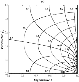
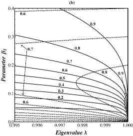
Figure 1: The map $(\alpha_{1},\alpha_{2})$ $\to$ $(\lambda,\beta_{1})$ in the chains engineered for the pure one-qubit PST (for instance, in the Ekert chain with $t_{0}=\pi$). Solid and dashed lines correspond to the constant values of the parameters, respectively, $\alpha_{2}$ and $\alpha_{1}$, appropriate values of these parameters are indicated in the picture. The variation intervals (46) of $\alpha_{i}$ are splitted into 10 equal segments, i.e., the parameter increment between the two neighboring lines is 0.1 in both families of curves. The solid line $\alpha_{2}=0$ coincides with the right vertical coordinate axis, the dashed line $\alpha_{1}=0$ is disrupted and coincides with the upper and lower horizontal coordinate axes. The solid and dashed lines with, respectively, $\alpha_{2}=1$ and $\alpha_{1}=1$ shrink to the point $(\lambda,\beta_{1})=(1,0)$. The properly scaled neighborhood of this point is depictured in Fig. (b). We keep the same gridding in all pictures below.

for the ideal case of the completely creatable receiver’s space. As mentioned above, this situation can be realized in the chains engineered for the PST. The Ekert chain can be considered as an example CDEL , then

$$D_{i}=\sqrt{i(N-i)}$$ (70)

in eq.(56), therewith $t_{0}=\pi$. In the case of homogeneous spin chain ($D_{i}\equiv D$, $i=1,\dots,N-1$, in eq.(56); we put $D=1$ for simplicity (dimensionless time $t$)), the map differs from that shown in Fig.1. We observe that the creatable region of the receiver’s space decreases very quickly with the chain length, as shown in Fig.2, where chains of 6, 60 and 120 nodes are considered at the time instants, respectively, $t_{0}=7.884$, 63.881 and 124.761.

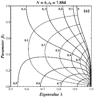
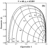
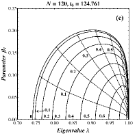
Figure 2: The map $(\alpha_{1},\alpha_{2})$ $\to$ $(\lambda,\beta_{1})$ in the homogeneous chains with $N=6$, 60, 120, at the time instants $t_{0}$ corresponding to the maximum of $p_{N1}$ (the highest-probability state transfer).

Figs.1 and 2 help us to select the needed region in the control parameter space $(\alpha_{1},\alpha_{2})$ to create the state inside of the required region of the creatable parameter-space $(\lambda,\beta_{1})$.

III Selection of creatable subregions.

We have considered a problem of maximal possible covering of the receiver’s state space. It is shown for Hamiltonian (56) that the maximal creatable region corresponds to the time instant $t_{0}$ of the highest-probability state transfer. Any deviation from $t_{0}$ reduces the creatable region. However, this unpleased phenomenon turns out to be useful if we would like to work only with a restricted subregion of the receiver’s state space without interacting with its remaining part. For instance, this problem appears in a ”branched” communication line when we need to share the creatable region among several senders, so that each sender works only with its own subregion. In fact, Fig.2 shows, that the creatable region of homogeneous chain of 120 nodes is restricted, roughly speaking, by the rectangle $0.74<\lambda\leq 1$, $0\leq\beta_{1}<0.21$. So, the region outside of this rectangle can be safely used for other purposes.

Now we describe the separation of several non-overlapping creatable subregions. Our results are based on the following observation. If we take $t_{1}<t_{0}$, then the conditions of Proposition 2 are broken, so that we do not cover the maximal creatable region varying the control parameters $\alpha_{1}$ and $\alpha_{2}$. Moreover, the parameter $R$ in formulas (25) and (27) can not take all values in interval (53) (remember that $t$ is fixed here, unlike Proposition 1). In general, the lower and upper boundaries appear:

$$q_{min}(t_{1})\leq R\leq q_{max}(t_{1}).$$ (71)

Thus, considering $K$ chains of different lengths $N_{i}$, $N_{1}<\dots<N_{K}$, and appropriate time instant $t_{i}$ such that

$$q^{i}_{min}(t_{i})>q^{i+1}_{max}(t_{i+1}),\;\;i=1,\dots,K-1,$$ (72)

we may select $K$ non-overlapping creatable subregions in the receiver’s state space. All these regions have the only common point $(\lambda,\beta_{1})=(1,0)$.

First, we consider the selective state creation using the homogeneous chains. In this case we use the time instants $t_{i}$ and the chain lengths $N_{i}$ as parameters selecting the proper creatable subregions. Combining both these parameters we can vary the creatable subregion in a needed way. Example of two particularly selected creatable subregions corresponding to $(N,t)=(6,9.375)$ and $(60,62.7)$ are shown in Fig. 3a.

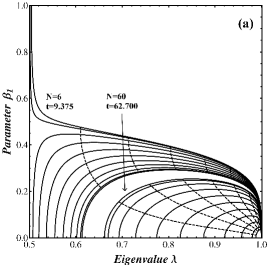
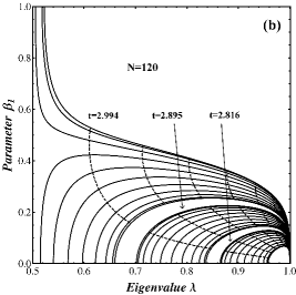
Figure 3: The selectivity in the remote state creation. Choosing the proper chain lengths and/or the time instants of the state registration we obtain different braid-shaped creatable regions. Gridding lines inside of each braid are the same as in Fig.1, i.e., the parameters $\alpha_{i}$, $i=1,2$ take values in interval (46). (a) The homogeneous spin chains of $N=6$ and 60 with the state-detecting time instants, respectively, $t=9.375$ and 62.7. (b) The Ekert chain with $N=120$ and the state-detecting time instants $t=2.994$, 2.895 and 2.816.

Next, we perform the above selection using the Ekert chain CDEL . In this case we can create different subregions using the chains of the same prescribed length $N$ and varying the time instants $t_{i}$ of the state registration. Example of three creatable subregions corresponding to the chain of $N=120$ spins and the registration time instants $t=2.994$, 2.895 and 2.816 are shown in Fig. 3b.

The privilege of homogeneous chains is that their creatable regions are restricted as shown in Fig.2, which reduces the possibility of ”parasitic” state creation from an ”alien” sender. For instance, the sender responsible for the lower region in Fig.3a ($N=60$) can not create the states in the upper selected region (corresponding to $N=6$) regardless of the values of the control parameters, this conclusion follows from comparison of Figs. 3a and 2b. Although the opposite is not true and 6-node chain can create the ”parasitic” states in the lower subregion of Fig.3.

IV Long distance eigenvalue creation in homogeneous and non-homogeneous chains

IV.1 Three types of creatable parameters.

In Secs.II.3, II.5 we show that the whole receiver’s state-space Z_2014 can not be remotely created using arbitrary spin chain. But are there equivalent obstacles for creation of each of three parameters $\lambda$, $\beta_{1}$ and $\beta_{2}$ of the receiver’s state space? It seamed out that all these parameters behave differently in the state creation process.

First of all, we shall emphasis the principal difference between the eigenvalue $\lambda$ and the eigenvector-parameters $\beta_{i}$, $i=1,2$. The latter have such an advantage that they, in principle, can be tuned to the required values by the local unitary transformation of the receiver (assuming that unitary transformations are applicable on the receiver side), which is a quantum-mechanics operation. Indeed, if we have created the receiver’s state in the form (17), i.e., $\rho^{B}=U^{B}\Lambda^{B}(U^{B})^{+}$, while the required state is $\rho^{req}=\tilde{U}^{B}\Lambda^{B}(\tilde{U}^{B})^{+}$ (for the one-qubit receiver, the unitary transformation $\tilde{U}^{B}$ has the form (21) with different parameters), then $\rho^{req}=\tilde{U}^{B}(U^{B})^{+}\rho^{B}U^{B}(\tilde{U}^{B})^{+}$, i.e., the mentioned above local transformation of the receiver reads:

$$U^{loc}=\tilde{U}^{B}(U^{B})^{+}.$$ (73)

Notice that the transformation $U^{loc}$ depends on the sender’s control parameters, which are included into $U^{B}$. Consequently, the receiver needs information about (some of) the control parameters to apply the proper $U^{loc}$. This information must be transfered from the sender to the receiver using some additional (classical) communication channel, similar to the teleportation algorithm. This means that, involving $U^{loc}$ into the state-creation algorithm, we lose the completely remote control of all parameters of the receiver state, except for the eigenvalues (matrix $\Lambda^{B}$) which can not be changed by $U^{loc}$. In this paper we do not consider the local transformations of the receiver as a part of the state-creation algorithm.

It is also shown in Sec. II.3 that the most reliable parameter is the phase $\beta_{2}$ Z_2014 , because any its value can be created using the phases $\varphi_{i}$, $i=1,2$, of the sender’s initial state. Moreover, this property of the parameter $\beta_{2}$ does not depend on the Hamiltonian governing the spin dynamics (this can be simply demonstrated). All this suggests us to consider this parameter as a preferable candidate for the carrier of quantum information.

Thus, the eigenvalue $\lambda$ turned out to be the most defenseless parameter, because (i) we are not able to create its arbitrary value (in general) and (ii) it can not be changed by the local unitary transformations of receiver. Therefore the eigenvalue is completely defined by the sender’s initial state and by the interaction Hamiltonian, and consequently the eigenvalue-creation deserves a special study.

Let us consider the $\lambda$-creation in more details using three types of chains: the homogeneous chain, the alternating chain and the chain engineered for the one-qubit PST (Ekert chain).

IV.2 Eigenvalue creation using Ekert chain, homogeneous and alternating chains

Considering the state-creation based on a spin chain of general position, the maximal variation interval (22) for $\lambda$ becomes compressed. The reason is pointed out in Sec.II.3, where the expression for $\lambda$ as a function of $R$ is represented, see eq.(25). It was shown that the left boundary of eigenvalue $\lambda_{l}=\frac{1}{2}$ can be created if $R>R_{min}=\frac{1}{\sqrt{2}}$, see eq.(41). Consequently, this boundary is achievable if only $R_{min}\leq r_{max}$ in eq.(58). This suggests us to introduce the parameter $\lambda^{cr}_{min}(N)$ indicating the minimal eigenvalue creatable on the receiver site as a characteristics of the chain.

Considering the homogeneous spin chain ($D_{i}=D_{1}=1$, $i=1,\dots,N-1$ in eq.(56)), we see from Fig.2 that $\lambda_{min}^{cr}(N)=\frac{1}{2}$ only if the chain is short enough (Fig.2a), unlike the long chains (Fig.2b,c). The general dependence of $\lambda^{cr}_{\min}$ on $N$ is shown in Fig.4, indicating that there is such the critical length $N_{c}^{hom}=34$ that

$$\lambda^{cr}_{min}>\frac{1}{2}\;\;{\mbox{for}}\;\;N>N_{c}^{hom}.$$ (74)

Figure 4: The homogeneous spin chains: the minimal creatable eigenvalue $\lambda^{cr}_{min}$ as a function of chain length $N$ .

Of course, $\lambda^{cr}_{min}(N)=\frac{1}{2}$ and does not depend on the chain length in the case of Ekert chain ($N_{c}^{PST}=\infty$). However, such chains are hard for realization, so that we are forced to look for alternative ways of increasing the parameter $N_{c}$.

A simple way to do that is using an alternating chain. In this case $D_{i}=D_{1}=1$, $i=1,3,5,\dots$ and $D_{i}=D_{2}=d$, $i=2,4,6,\dots$ in eq.(56). Therewith $d$ is called the alternation parameter. The results of our calculations for the chain with even number of nodes are collected in Fig.5. To simplify calculations we put $\alpha_{2}=0$ in this subsection. Using variable parameter $\alpha_{2}$ we would only slightly modify figures without changing the parameter $N_{c}$.

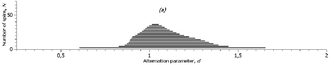
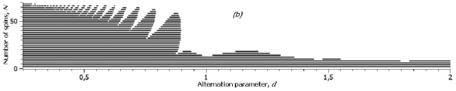
Figure 5: The eigenvalue creation in the alternating spin chains with even $N$ over the different time intervals. Lines (or spots) correspond to the creation of any $\lambda$ from the interval $\frac{1}{2}\leq\lambda\leq 1$ for the appropriate $N$ and $d$. The envelope of each figure represents the critical length $N_{c}^{even}$ as a function of the dimerization parameter $d$. (a) $0\leq t\leq 1.3N\min\Big{(}d,\frac{1}{d}\Big{)}$, $(N_{c}^{even})_{max}=36>N_{c}^{hom}=34$. (b) $1.3\min\Big{(}d,\frac{1}{d}\Big{)}<t\leq 1.5N\max\Big{(}d,\frac{1}{d}\Big{)}$, $(N_{c}^{even})_{max}=68>N_{c}^{hom}$ .

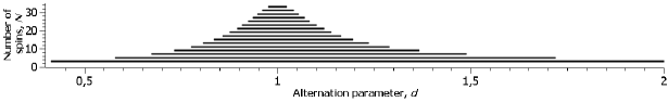
Figure 6: The same as Fig.5 for the chain with odd $N$ and the time interval $0\leq t\leq 3N\min\Big{(}d,\frac{1}{d}\Big{)}$; $(N_{c}^{odd})_{max}=33<N_{c}^{hom}$.

The chain with even number of nodes is considered in Fig.5. The parameter $R$ responsible for the $\lambda$-creation takes its critical value $\frac{1}{\sqrt{2}}$ inside of different time intervals depicted on Figs. 5a,b. The lines (or spots) mean that any $\lambda$ from the interval $\frac{1}{2}\leq\lambda\leq 1$ can be created for the proper $N$ and $d$. The envelopes of these figures give the parameter $N_{c}^{even}$ as a function of $d$. The most reasonable time interval, $0\leq t\leq 1.3\min\Big{(}d,\frac{1}{d}\Big{)}$, is depicted in Figs.5a: the alternation allows us to increase the length $N_{c}$ till $N_{c}^{even}=36$. More significant increase in $N_{c}$ is observed over the second time interval $1.3\min\Big{(}d,\frac{1}{d}\Big{)}<t\leq 1.5\max\Big{(}d,\frac{1}{d}\Big{)}$ shown in Figs.5b (the numerical coefficients $1.3$ and $1.5$ are empiric). In this case $N_{c}^{even}=68$ which is twice bigger than $N_{c}^{hom}$. This results from the chain ”dimerization” with decrease in the alternation parameter $d$. We see that the function $N_{c}^{even}(d)$ is not unique for $d<1$ if $R$ achieves its critical value $\frac{1}{\sqrt{2}}$ over the time interval corresponding to Fig.5b.

The case of odd $N$ is not interesting because it does not yield any increase of the critical length in comparison with the homogeneous chain ($N_{c}^{odd}=33<N_{c}^{hom}$), as shown in Fig.6.

V Conclusions

In this paper we study several aspects of the remote state creation using the homogeneous, Ekert and alternating spin-1/2 chains. To simplify calculation, we require the commutation condition (2) for the Hamiltonian and one-spin excitation initial state. Based on these requirements are the following results.

1. The receiver’s density matrix can be simply expressed in terms of the probability amplitudes. These amplitudes are the characteristics of the transmission line known in advance, Secs.II.1, II.2.

2. Three parameters of the creatable one-qubit state-space can be referred to as the phase and amplitude of the eigenvector and the eigenvalue. We show that an arbitrary eigenvector’s phase can be created using the proper values of the control parameters (Sec.II.3), the eigenvector’s amplitude can be tuned by the unitary transformation of the receiver, while the eigenvalue is most hard creatable and thus deserves the special consideration, Sec.IV.

3. Being the most reliably creatable, the eigenvector’s phase (parameter $\beta_{2}$) is a preferable candidate for the quantum information carrier in quantum communication lines.

In addition, the following results were obtain for nearest-neighbor XY-Hamiltonian (56).

1. The arbitrary parameters of the two-qubit pure sender’s initial state are the control parameters establishing the complete local control of the receiver’s creatable region at the properly fixed time instant of the state registration, Secs.II, III.

2. The maximal creatable region corresponds to the time instant associated with the highest-probability state transfer (although this probability may be far from unit, i.e., ”highest” does not mean ”high”). The creatable region decreases very quickly with the chain length of a homogeneous chain. As anticipated in Z_2014 , the complete state space of the one-qubit receiver can be created only in the spin chain engineered for the pure one-qubit PST, Secs.II.3, II.5.

3. The map (control parameter-space) $\to$ (creatable parameter-space) is numerically described and depicted in Figs.1, 2, thus helping to choose the control parameters needed to create a particular receiver’s state, Sec.II.5. Everywhere in Figs.1-3 we use the same gridding of the parameter space $(\alpha_{1},\alpha_{2})$.

4. Choosing different lengths of the homogeneous chain and different time-instants of the state registration we can select the needed creatable subregion. A similar result can be achieved using the Ekert chain of a fixed length and different time-instants of the state registration, Sec.III.

5. Considering the process of the remote eigenvalue creation we show that the arbitrary eigenvalue can be created through the homogeneous spin chain of up to 34 nodes, through the alternating chain of up to 68 nodes and through the Ekert chain of arbitrary length, Sec.IV.2.

Among the aspects deserving deeper study we mention (i) the transformation of created states using the tool of local (non-unitary) operations; (ii) the robustness of state-creation with respect to chaotic permutations and model imperfections; in particular, the effect of remote spin interactions has to be clarified; (iii) the model with two-excitation initial state (instead of the single-excitation one) has to be explored.

We shall also notice that the creation and evolution of quantum correlations is another direction of quantum information processing stimulating intensive investigations (for instance, see refs.DSC ; LBAW ; NLLZ ; ZC ; SXSZDWHCKW ; RDL ). Currently, the quantum entanglement Wootters ; HW ; AFOV ; HHHH and the quantum discord Z0 ; HV ; OZ ; Z are widely accepted measures of quantum correlations. The remote creation of entangled quantum states and states with quantum discord is one more problem postponed for further study.

Authors thank Prof. E. B. Fel’dman, Dr. S. I. Doronin and Dr. A. N. Pyrkov for useful discussion and comments. This work is partially supported by the program of RAS ”Element base of quantum computers”, by the Russian Foundation for Basic Research, grants No.15-07-07928 and No.13-03-00017 (A.I.Z.).

References

- (1) S. Bose, Phys. Rev. Lett. 91, 207901 (2003)
- (2) M.Christandl, N.Datta, A.Ekert and A.J.Landahl, Phys.Rev.Lett. 92, 187902 (2004)
- (3) C.Albanese, M.Christandl, N.Datta and A.Ekert, Phys.Rev.Lett. 93, 230502 (2004)
- (4) P.Karbach and J.Stolze, Phys.Rev.A 72, 030301(R) (2005)
- (5) G.Gualdi, V.Kostak, I.Marzoli and P.Tombesi, Phys.Rev. A 78, 022325 (2008)
- (6) A.Wójcik, T.Luczak, P.Kurzyński, A.Grudka, T.Gdala, and M.Bednarska Phys. Rev. A 72, 034303 (2005)
- (7) G.M.Nikolopoulos and I.Jex, eds., Quantum State Transfer and Network Engineering, Series in Quantum Science and Technology, Springer, Berlin Heidelberg (2014)
- (8) J.Stolze, G. A. Álvarez, O. Osenda, A. Zwick in Quantum State Transfer and Network Engineering. Quantum Science and Technology, ed. by G.M.Nikolopoulos and I.Jex, Springer Berlin Heidelberg, Berlin, p.149 (2014)
- (9) J.Zhang, G. L. Long, W. Zhang, Zh. Deng, W. Liu, and Zh. Lu, Phys.Rev.A 72, 012331 (2005)
- (10) G. De Chiara, D. Rossini, S. Montangero, R. Fazio, Phys. Rev. A 72, 012323 (2005)
- (11) A. Zwick, G.A. Álvarez, J. Stolze, O. Osenda, Phys. Rev. A 84, 022311 (2011)
- (12) A. Zwick, G.A. Álvarez, J. Stolze, O. Osenda, Phys. Rev. A 85, 012318 (2012)
- (13) A. Zwick, G.A. Álvarez, J. Stolze, O Osenda, Quant. Inf. Comput. 15, 582 (2015)
- (14) W.K. Wootters,, Phys. Rev. Lett. 80, 2245 (1998)
- (15) S.Hill and W.K.Wootters, Phys. Rev. Lett. 78, 5022 (1997)
- (16) A.Peres, Phys. Rev. Lett. 77, 1413 (1996)
- (17) L.Amico, R.Fazio, A.Osterloh and V.Ventral, Rev. Mod. Phys. 80, 517 (2008)
- (18) R.Horodecki, P.Horodecki, M.Horodecki and K.Horodecki, Rev. Mod. Phys. 81, 865 (2009)
- (19) S.I.Doronin, E.B.Fel’dman, and A.I.Zenchuk, Phys. Rev. A 79, 042310 (2009)
- (20) S.I.Doronin, A.I.Zenchuk, Phys. Rev. A 81, 022321 (2010)
- (21) L. Banchi, T. J. G. Apollaro, A. Cuccoli, R. Vaia, and P. Verrucchi, Phys.Rev.A 82, 052321 (2010)
- (22) L. Banchi, T. J. G. Apollaro, A. Cuccoli, R. Vaia and P. Verrucchi, New J. Phys. 13, 123006 (2011)
- (23) P. Lorenz, J. Stolze, Phys. Rev. A 90, 044301 (2014)
- (24) L.Banchi, A. Bayat, P. Verrucchi, and S.Bose, Phys.Rev.Let. 106, 140501 (2011)
- (25) B. Chen, and Zh. Song, Sci. China-Phys., Mech. Astron 53, 1266 (2010)
- (26) L. Banchi, Eur. Phys. J. Plus 128, 137 (2013)
- (27) W. Qin, J. L. Li, G. L. Long, Chin. Phys. B 24, 040305 (2015)
- (28) Zh. Yang, M. Gao, W. Qin, arXiv:1503.06274
- (29) W. Qin, Ch. Wang, and X. Zhang, Phys.Rev.A 91, 042303 (2015)
- (30) A.I.Zenchuk, J. Phys. A: Math. Theor. 45 (2012) 115306
- (31) A.I.Zenchuk, Phys. Rev. A 90, 052302(13) (2014)
- (32) E.I.Kuznetsova and E.B.Fel’dman, J.Exp.Theor.Phys. 102, 882 (2006)
- (33) E.I.Kuznetsova and A.I.Zenchuk, Phys.Lett.A 372, pp.6134-6140 (2008)
- (34) E.B.Fel’dman and A.I.Zenchuk, Phys. Lett. A 373 (2009) 1719
- (35) M.Zukowski, A.Zeilinger, M.A.Horne, A.K.Ekert, Phys. Rev. Lett. 71, 4287 (1993)
- (36) D.Bouwmeester, J.-W. Pan, K.Mattle, M.Eibl, H.Weinfurter, and A. Zeilinger, Nature 390, 575 (1997)
- (37) D. Boschi, S. Branca, F. De Martini, L. Hardy, and S. Popescu, Phys. Rev. Lett. 80, 1121 (1998)
- (38) N.A.Peters, J.T.Barreiro, M.E.Goggin, T.-C.Wei, and P.G.Kwiat, Phys.Rev.Lett. 94, 150502 (2005)
- (39) N.A.Peters, J.T.Barreiro, M.E.Goggin, T.-C.Wei, and P.G.Kwiat in Quantum Communications and Quantum Imaging III, ed. R.E.Meyers, Ya.Shih, Proc. of SPIE 5893 (SPIE, Bellingham, WA, 2005)
- (40) B.Dakic, Ya.O.Lipp, X.Ma, M.Ringbauer, S.Kropatschek, S.Barz, T.Paterek, V.Vedral, A.Zeilinger, C.Brukner, and P.Walther, Nat. Phys. 8, 666 (2012).
- (41) G.Y. Xiang, J.Li, B.Yu, and G.C.Guo Phys. Rev. A 72, 012315 (2005)
- (42) C.H.Bennett, G.Brassard, C.Crépeau, R.Jozsa, A.Peres, and W.K.Wootters, Phys. Rev. Lett. 70, 1895 (1993)
- (43) B.Yurke, D.Stoler, Phys. Rev. A 46, 2229 (1992)
- (44) B.Yurke, D.Stoler, Phys. Rev. Lett. 68, 1251 (1992)
- (45) C.H.Bennett, D.P.DiVincenzo, P.W.Shor, J.A.Smolin, B.M.Terhal, and W.K.Wootters, Phys.Rev.Lett. 87, 077902 (2001); Erratum, C.H.Bennett, D.P.DiVincenzo, P.W.Shor, J.A.Smolin, B.M.Terhal, and W.K.Wootters, Phys. Rev. Lett. bf 88, 099902(E) (2002)
- (46) C.H.Bennett, P.Hayden, D.W.Leung, P.W.Shor, and A.Winter, IEEE Transetction on Information Theory 51, 56 (2005)
- (47) G.L.Giorgi, Phys. Rev. A 88, 022315 (2013)
- (48) W. H. Zurek, Ann. Phys.(Leipzig), 9, 855 (2000)
- (49) L.Henderson and V.Vedral J.Phys.A:Math.Gen. 34, 6899 (2001)
- (50) H.Ollivier and W.H.Zurek, Phys.Rev.Lett. 88, 017901 (2001)
- (51) W. H. Zurek, Rev. Mod. Phys. 75, 715 (2003)
- (52) Datta, A., Shaji, A., Caves, C.M., Phys. Rev. Lett. 100, 050502 (2008)
- (53) Lanyon, B.P., Barbieri, M., Almeida, M.P., White, A.G., Phys. Rev. Lett. 101, 200501 (2008)
- (54) W.J.Nie, Yu.H.Lan, Yo.Li, and Sh.Ya.Zhu, Sci.China-Phys., Mech. Astron 57, 2276 (2014)
- (55) P. Zhang, B. You, and L.-X. Cen, Chin. Sci. Bull., 59, 3841 (2014)
- (56) J.X. Sci, W. Xu, G. Sun et al, Chin. Sci. Bull. 59, 2547 (2014)
- (57) S. Rodriques, N. Datta, and P. J. Love, Phys. Rev. A 90, 012340 (2014)