DDA: Cross-Session Throughput Prediction with Applications to Video Bitrate Selection

Abstract

User experience of video streaming could be greatly improved by selecting a high-yet-sustainable initial video bitrate, and it is therefore critical to accurately predict throughput before a video session starts. Inspired by previous studies that show similarity among throughput of similar sessions (e.g., those sharing same bottleneck link), we argue for a cross-session prediction approach, where throughput measured on sessions of different servers and clients is used to predict the throughput of a new session. In this paper, we study the challenges of cross-session throughput prediction, develop an accurate throughput predictor called DDA, and evaluate the performance of the predictor with real-world datasets. We show that DDA predicts throughput more accurately than simple predictors and conventional machine learning algorithms; e.g., DDA’s 80%ile prediction error of DDA is $\geq$ 50% lower than other algorithms. We also show that this improved accuracy enables video players to select a higher sustainable initial bitrate; e.g., compared to initial bitrate without prediction, DDA leads to $4\times$ higher average bitrate.

1 Introduction

Many Internet applications can benefit from estimating the client-server throughput. For instance, accurate estimation of throughput helps content distribution networks to redirect clients to servers that provide the best performance. Similarly, peer-to-peer networks select the best peers based on the estimation of their throughput performance.

Our focus in this paper is on the initial video bitrate selection when a video player starts. A video player should ideally pick the highest initial bitrate that is sustainable (i.e., below the throughput), in order to ensure desired user experience of video streaming. Existing approaches to initial bitrate selection, however, are inefficient. Table 1 shows measured anecdotal evidence of such inefficiencies from several commercial providers. Fixed-bitrate players that use the same bitrate for the whole video session often intentionally use low bitrate to prevent mid-stream rebuffering (e.g., NFL, Lynda). Even if bitrate can be adapted midstream (e.g., [8, 5, 18]) the player often conservatively starts with a low bitrate and takes a significant time to reach the optimal bitrate (e.g., Netflix). Furthermore, for short video clips such adaptation may not reach the desired bitrate before the video finishes (e.g., Vevo music clips).

Streaming protocol	Examples	Limitations	How throughput prediction helps
Fixed bitrate	NFL,Lynda, NYTimes	Too low bitrate, a few chunks are	Higher bitrate with no re-buffering or
Adaptive bitrate	ESPN,Vevo, Netflix	wasted to probe throughput	long startup time

Table 1: Limitations of today’s video players and how they benefit from throughput prediction. www.lynda.com uses fixed bitrate of 520Kbps (360p) by default. Netflix (www.netflix.com/WiMovie/70136810?tr kid=439131) takes roughly 25 seconds to adapt from the initial bitrate (560Kbps) to the highest sustainable bitrate (3Mbps).

The importance of initial bitrate selection (e.g., avoid users quitting) naturally makes a case for a predictive approach – predicting the TCP throughput before a session starts. Inspired by prior work on shared measurements [25], we explore a cross-session approach where the TCP throughput of other sessions is used to predict the throughput of a new session. Intuitively, we want to build a prediction model for each client-server pair as a function of key session features available to us (e.g., ISP, connection type). This has the natural advantage that it incurs no additional measurement overhead and leverages all available sessions even if there is no history between same client and server. While this idea is not particularly new, we believe that revisiting this is timely in light of the need for video quality optimization and the availability of large-scale throughput measurements to many video service providers.

However, it is challenging to predict throughput accurately based on other sessions’ throughput, because of a complex underlying interaction between session features and throughput. There are two manifestations of this complexity (see

2 LABEL:

sec:analysis for more details). First, throughput usually can only be accurately predicted by combination of multiple features. For instance, only sessions from a particular ISP-server-device combination may have similarly low throughput, but the individual ISP, server or device may manifest no problem. Second, the best feature combination to predict throughput differs across sessions. For instance, for sessions in one ISP, the best feature to predict their throughput is last-mile connection (e.g., last hope is the bottleneck), while for those in another ISP, the best feature is time of day (e.g., due to a strong diurnal pattern).

To address these challenges, we present DDA (Data-Driven Aggregation), which predicts each session’s throughput by an expressive prediction model that captures temporal similarity (e.g., sessions happening within a smaller time window) and spatial similarity (e.g., sessions matching more features with the session under prediction) between previously observed sessions and the session under prediction. Such prediction models allow DDA to predict throughput accurately by aggregating sessions with similar throughput. Instead of using a single prediction model, DDA customizes the prediction model for each session under prediction. To pick the prediction model that yields high prediction accuracy for each session, DDA adopts a data-driven approach and learns the best prediction model by searching for the best prediction model to similar existing history sessions.

In summary, this paper makes three key contributions.

• First, we use a dataset of real-world throughput measurement of 9.9 million sessions to show the challenges of cross-session throughput prediction (

  3 LABEL:

  sec:analysis).

• Second, we present a concrete cross-session throughput predictor, DDA that addresses the above challenges (

  4 LABEL:

  sec:algorithm).

• Finally, our evaluation based on two real-world datasets shows that DDA can predict throughput more accurately than simple predictors and conventional machine learning algorithms, and that due to more accurate throughput prediction, DDA allows a video player to select a higher-yet-sustainable initial bitrate (

  5 LABEL:

  sec:eval).

6 Related Work

At a high-level, our work is related to prior work in measuring Internet path properties, bandwidth measurements, and video-specific bitrate selection. With respect to prior measurement work, our key contribution is showing a practical data-driven approach for throughput prediction. In terms of video, our predictive approach offers a more systematic bitrate selection mechanism.

Measuring path properties:  Studies on path properties have shown prevalence and persistence of network bottlenecks (e.g., [13]), constancy of various network metrics [31], longitudinal patterns of cellular performance (e.g., [22]), and spatial similarity of network performance (e.g., [10]). While DDA is inspired by these insights, it addresses a key gap because these efforts fall short of providing a prescriptive algorithm for throughout prediction.

Bandwidth measurement:  Unlike prior “path mapping” efforts (e.g., [19, 25, 24, 11]), DDA uses a data-driven model based on available session features (e.g., ISP, device). Specifically, video measurements are taken within a constraint sandbox environment (e.g., browser) that do not offer interface for path information (e.g., traceroute). Other approaches use packet-level probing to estimate the end-to-end performance metrics (e.g., [23, 14, 26, 16]). Unlike DDA, these require additional measurement and often need full client/server-side control which is often infeasible in the wild. A third class of approaches leverages the history of the same client-server pair (e.g., [29, 17, 27, 21, 12]). However, they are less reliable when the available history of the same client and server is sparse.

Bitrate selection:  Choosing high and sustainable bitrate is critical to video quality of experience [9]. Existing methods (e.g., [20, 18]) require either history measurement between the same client and server or the player to probe the server to predict the throughput. In contrast, DDA is able to predict throughput before a session starts. Other approaches include switching bitrate midstream (e.g., [15, 28, 30]) but do not focus on the initial bitrate problem which is the focus of DDA.

7 Datasets

We use two datasets of HTTP throughput measurement to evaluate DDA’s performance: (i) a primary dataset collected by FCC’s Measuring Broadband American Platform [4] in September 2013, and (ii) a supplementary dataset collected by a major VoD provider in China.

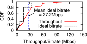
Figure 1: Distribution of throughput in the FCC dataset

FCC dataset:  This dataset consists of 9.9 million sessions and is collected from 6204 clients in US spanning 17 ISPs. In each test, a client set up an HTTP connection with one of the web servers for a fixed duration of 30 seconds and attempted to download as much of the payload as possible. It also recorded average throughput at 5 second intervals during the test. The test used three concurrent TCP connections to ensure the line was saturated. Reader may refer to [1] for more details on the methodology.

Figure 1 shows the throughput distribution of all sessions. It also shows the distribution of ideal bitrate (i.e., highest bitrate chosen from {0.016, 0.4, 1.0, 2.5, 5.0, 8.0, 16.0, 35.0}Mbps below the throughput). With perfect throughput prediction, we should be able to achieve average bitrate of 26.9Mbps with no session suffering from re-buffering. Compared to the fixed initial bitrate (e.g., 2.5Mbps) used today, this suggests a large room of improvement.

The clients represent a wide spatial coverage of ISPs, geo-locations, and connection technology (see Table 2). Although the number of targets are relatively small, the setting is very close to what real-world application providers face – the clients are widely distributed while the servers are relatively fewer. In addition, its measurement frequency (i.e., each client fetching content from each server once every hour) provides a unique opportunity to test the prediction algorithms’ sensitivity to different measurement frequency. For instance, to emulate the effect of reduced data, we take one (the first) 5-second throughput sample from each test, and then randomly drop (e.g., 90% of) the available measurements to simulate a dataset where each client accesses a server less frequently (e.g., in average once every 10 hours).

Feature	Description	# of unique values
ClientID	Unique ID associated to a client	6204
ISP	ISP of client (e.g., AT&T)	17
State	The US state where the client is located	52
Technology	The connection technology (e.g., DSL)	5
Target	The server-side identification	30
Downlink	Advertised download speed of the last connection (e.g., 15MB/s)	36
Uplink	Advertised upload speed of the last connection (e.g., 5MB/s)	25

Table 2: Basic statistics of the FCC dataset.

Supplementary VoD dataset:  As a supplementary dataset, we use throughput dataset of 0.8 millions VoD sessions, collected by a major video content provider in China. Each video session has the average throughput and a set of features, that are different from the FCC dataset, including content name, user geolocation, user ID and server IP. This provides an opportunity to test the sensitivity of the algorithms to different sets of available features.

8 Simple Predictors are Not Sufficient

This section starts by showing that simple predictors fail to yield desirable prediction accuracy, and then shows fundamental challenges of cross-session throughput prediction.

• First, we consider the last-mile predictor, which uses sessions with the same $\mathit{downlink}$ feature (see definition in Table 2) to predict a new session’s throughput. This is consistent to the conventional belief that last-mile connection is usually the bottleneck. However, Figure 2(a) and 2(b) show substantial prediction error, especially on the tail where at least 20% of sessions have more than 20% error (Figure 2(b)). To put it into perspective, if a player chooses bitrate based on throughput prediction that is 20% higher or lower than the actual, the video session will experience mid-stream re-buffering or under-utilize the connection. Finally, Figure 2(c) and 2(d) show that the prediction error is two-sided, suggesting that simply adding or multiplying the prediction by a constant factor will not fix the high prediction error.

  

  (a) Non-normalized absolute

  

  (b) Normalized absolute

  

  (c) Non-normalized signed

  

  (d) Normalized signed

  Figure 2: Prediction error of the last-mile predictor

• Second, we consider the last-sample predictor, which uses the throughput of the last session of the same client-target pair to predict the throughput of a future session. However, the last-sample predictor is not reliable as the last sample is too sparse and noisy to offer reliable and accurate prediction. Figure 3 shows that, similar to the last-mile predictor, (i) the prediction error, especially on the tail, is not desirable – more than 25% of sessions have more than 20% normalized prediction error, and (ii) the prediction error is two-sided, suggesting the prediction error cannot be fixed by simply adding or multiplying the prediction with a constant factor.

  

  (a) Non-normalized absolute

  

  (b) Normalized absolute

  

  (c) Non-normalized signed

  

  (d) Normalized signed

  Figure 3: Prediction error of last-sample predictor

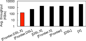
(a) The average throughput of sessions matching all and a subset of three features: $\mathit{ISP=}$ Frontier, $\mathit{Technology=}$ DSL and $\mathit{Target=}$ samknows1.lax9.level3.net (X). Time: 18:00-00:00 UTC, Oct 7, 2013

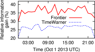
(b) The relative information gain of $\mathit{Target}$ in two ISPs over time.

Figure 4: Two manifestations of the high complex interaction between session features and the throughput.

Challenges:  The fundamental challenge to produce accurate prediction is the complex underlying interactions between session features and their throughput. In particular, there are two manifestations of such high complexity.

First, the simple predictors are both based on single feature (e.g., downlink or time), while combinations of multiple features often have a much greater impact on throughput than individual features. This can be intuitively explained as the throughput is often simultaneously affected by multiple factors (e.g., the last-mile connection, server load, backbone network congestion, etc), and that means sessions sharing individual features may not have similar throughput. Figure 4(a) gives an example of the effect of feature combinations. It shows the average throughput of sessions of ISP Frontier using DSL fetching target samknows1.lax9.level3.net, and average throughput of sessions having same values on one or two of the three features. The average throughput when all three features are specified is at least 50% lower than any of other cases. Thus, to capture such effect, the prediction algorithm must be expressive to combine multiple features.

Second, the simple predictors both use same feature to all sessions, but the impact of same features on different sessions could be different. For instance, throughput is more sensitive to last-mile connection when it is unstable (e.g., Satellite), and it depends more to ISP during peak hours when the network tends to be the bottlenecks. Figure 4(b) shows a real-world example. Relative information gain is often used to quantify how useful a feature is used for prediction. The figure shows the relative information gain of feature $\mathit{Target}$ on the throughput of sessions in two ISPs over time. It shows that the impact of the same feature varies across sessions in different hours and in different ISPs.

We will see in

9 LABEL:

sec:eval that due to the complex underlying interactions between features and throughput, it is non-trivial for conventional machine learning algorithms (e.g., decision tree, naive bayes) to yield high accuracy.

10 Predicting Throughput Using DDA

In this section, we present the DDA approach that yields accurate throughput prediction (

11 LABEL:

sec:eval). We start with an intuitive description of DDA before formally describing the algorithm.

11.1 Insight of DDA

At a high level, DDA finds for any session $\mathit{s}$ a prediction model – a pair of features and time range, which is used to aggregate history sessions that match the specific features with $\mathit{s}$ and happened in the specific range.

To motivate how DDA maps a session to a prediction model, let us consider two strawmen of session-model mapping shown in Figure 5. The first strawman maps each session $\mathit{s}$ to the “Nearest Neighbor” prediction model (dash arrows), which aggregates only history sessions matching all features with $\mathit{s}$ and happening in very short time (e.g., 5 minute) before $\mathit{s}$. Theoretically, “Nearest Neighbor” model should be highly accurate as it represents sessions that are the most similar to $\mathit{s}$, but history sessions meeting this requirement are too sparse to provide reliable prediction. Alternatively, one can map any $\mathit{s}$ to the “Global” prediction model (dot arrows), which aggregates all history sessions regardless of their features or happening time. While “Global” model is highly reliable as it has substantial samples in history, the accuracy is low because it does not capture the effect of feature combination introduced in the last section.

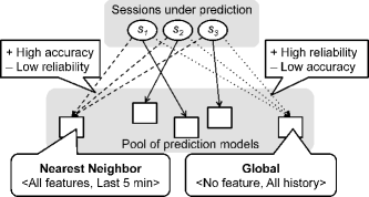
Figure 5: Mapping between sessions under prediction and prediction models.

Ideally, we would like achieve both high accuracy and high reliability. To this end, DDA (shown by solid arrows in Figure 5) differs from the above strawmen in two important aspects. First, DDA finds for a given session a prediction model between the Nearest Neighbor and Global prediction models, so that it strikes a balance between being closer to Nearest Neighbor for accuracy and being closer to Global for reliability. The resulting prediction model should be expressive (e.g., have more features) and yet have enough samples to offer a reliable prediction. Second, instead of mapping all sessions to the same prediction model, DDA maps different sessions to different prediction models, which allows DDA to address inherent heterogeneity that the same feature has different impact on different sessions.

11.2 Design of DDA

Overall workflow:  DDA uses two steps to predict the throughput of a new session $\mathit{s}$.

• First, DDA learns a prediction model $\mathit{M}^{\mathit{*}}_{\mathit{s}}$ based on history data. A prediction model is a pair of feature combination and time range.

• Second, DDA estimates $\mathit{s}$’s throughput by the median throughput of sessions in $\mathit{Agg(\mathit{M}^{\mathit{*}}_{\mathit{s}},\mathit{s})}$ that match $\mathit{s}$ on the feaures of $\mathit{M}^{\mathit{*}}_{\mathit{s}}$ and are in the time range of $\mathit{M}^{\mathit{*}}_{\mathit{s}}$. I.e., DDA’s prediction is $\mathit{Pred(\mathit{s})}=\mathit{Median}(\mathit{Agg(\mathit{M}^{\mathit{*}}_{\mathit{s}},\mathit{s})})$.

Learning of prediction model:  First, DDA learns a prediction model $\mathit{M}^{\mathit{*}}_{\mathit{s}}$ based on history data from a pool of all possible prediction models, i.e., pairs of all feature combinations (i.e., $2^{n}$ subsets of $n$ features in Table 2) and possible time windows. Specifically, the possible time windows include time windows of certain history length (i.e., last 10 minutes to last 10 hours) and those of same time of day/week (i.e., same hour of day in the last 1-7 days or same hour of week in the last 1-3 weeks).

The objective of $\mathit{M}^{\mathit{*}}_{\mathit{s}}$ is to minimize the prediction error, $\mathit{Err(\mathit{Pred(\mathit{s})},\mathit{\mathit{s}_{w}})}=\frac{|\mathit{Pred(\mathit{s})}-\mathit{\mathit{s}_{w}}|}{\mathit{\mathit{s}_{w}}}$, where $\mathit{\mathit{s}_{w}}$ is the actual throughput of $\mathit{s}$. That is,

$$\mathit{M}^{\mathit{*}}_{\mathit{s}}=\operatorname*{arg\,min}_{\mathit{M}}\mathit{Err(\mathit{Median}(\mathit{Agg(\mathit{M},\mathit{s})}),\mathit{\mathit{s}_{w}})}$$ (1)

Rather than solving Eq 1 analytically, DDA takes a data-driven approach and finds the best prediction model over a set of history sessions $\mathit{\mathit{Est}(\mathit{s})}$ (defined shortly). Formally, the process can be written as following:

$$\mathit{M}^{\mathit{*}}_{\mathit{s}}=\operatorname*{arg\,min}_{\mathit{M}}\frac{1}{|\mathit{\mathit{Est}(\mathit{s})}|}\sum_{\mathit{s}^{\prime}\in\mathit{\mathit{Est}(\mathit{s})}}\mathit{Err(\mathit{Median}(\mathit{Agg(\mathit{M},\mathit{s}^{\prime})}),\mathit{\mathit{s}^{\prime}_{w}})}$$ (2)

$\mathit{\mathit{Est}(\mathit{s})}$ should include sessions that are likely to share the best prediction model with $\mathit{s}$. In DDA, $\mathit{\mathit{Est}(\mathit{s})}$ consists of sessions that match features $\mathit{Target}$, $\mathit{ISP}$, $\mathit{Technology}$ and $\mathit{Downlink}$ with $\mathit{s}$ and happened within 4 hours before $\mathit{s}$.

Estimating throughput:  Second, DDA estimates $\mathit{s}$’s throughput by the learned prediction model $\mathit{M}^{\mathit{*}}_{\mathit{s}}$. To make the prediction $\mathit{Pred(\mathit{s})}$ reliable, DDA ensures that $\mathit{Pred(\mathit{s})}$ is based on a substential amount of sessions in $\mathit{Agg(\mathit{M}^{\mathit{*}}_{\mathit{s}},\mathit{s})}$. Therefore, if $\mathit{M}^{\mathit{*}}_{\mathit{s}}$ yields $\mathit{Agg(\mathit{M}^{\mathit{*}}_{\mathit{s}},\mathit{s})}$ with less than 20 sessions, DDA will remove that model from the pool and learn the prediction model as in the first step again. We have also found that for some pairs of client and server, DDA’s prediction error is one-sided. For instance, the throughput of a particular client-server pair is 1Mbps, while the best prediction model always predicts 2Mbps (i.e., a one-sided 100% error). We compensate this error by changing $\mathit{Median}(S)$ to $\mathit{Median}(S,k)$ which reports the median of throughput in $S$ times a factor $k$. To train a proper value of $k$, DDA first uses Eq 2 to learn $\mathit{M}^{\mathit{*}}_{\mathit{s}}$ by assuming $k=1$, and then, DDA trains the best factor $k^{\mathit{*}}_{\mathit{s}}$ for $\mathit{s}$ as follows:

$$k^{\mathit{*}}_{\mathit{s}}=\operatorname*{arg\,min}_{k}\frac{1}{|\mathit{\mathit{Est}(\mathit{s})}|}\sum_{\mathit{s}^{\prime}\in\mathit{\mathit{Est}(\mathit{s})}}\mathit{Err(\mathit{Median}(\mathit{Agg(\mathit{M}^{\mathit{*}}_{\mathit{s}},\mathit{s}^{\prime})},k),\mathit{\mathit{s}^{\prime}_{w}})}$$

where $k$ is chosen from 0 to 5. Finally, the prediction made by DDA will be $\mathit{Median}(\mathit{Agg(\mathit{M}^{\mathit{*}}_{\mathit{s}},\mathit{s})},k^{\mathit{*}}_{\mathit{s}})$.

12 Evaluation

This section evaluates the prediction accuracy of DDA (

13 LABEL:

subsec:accuracy-eval) and how much DDA improves video bitrate (

14 LABEL:

subsec:bitrate-eval). Overall, our findings show the following:

• DDA can predict more accurately than other predictors.

• With higher accuracy, DDA can select better bitrate.

14.1 Prediction accuracy

Methodology:  As points of comparison, we use implementations of Decision Tree (DT) and Naive Bayes (NB) with default configurations in weka, a popular ML tool [7]. For a fair comparison, all algorithms use the same set of features. We also compare them with last-mile predictor (LM) and last-sample predictor (LS), introduced in

15 LABEL:

sec:analysis. We update the model of other algorithms in a same way as DDA: for each session under prediction, we use all available history data before it as the train data. Each session’s timestamp is grouped into 10-minute intervals and used as discrete time feature. By default, we use absolute normalized error (

16 LABEL:

sec:algorithm) as the metric of prediction error, and the results are based on the FCC dataset, unless specified otherwise.

Distribution of prediction error:  Figure 6 shows the distribution of prediction error of DDA and other algorithms. DDA outperforms all algorithms, especially on the tail of prediction error. For the FCC dataset (Figure 6(a)), 80%ile prediction error of DDA is 50% to 80% lower than that of other algorithms, and DDA has less than 20% sessions with more than 10% prediction error, while all other algorithms have at least 30% session with more than 10% error. While the VoD dataset in general has higher prediction error than the FCC dataset (due to the lack of some features such as last-connection and longitudinal information), DDA still outperforms other algorithms, showing that DDA is robust to the available features.

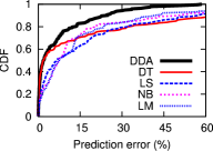
(a) FCC

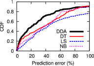
(b) VoD China

Figure 6: CDF of prediction error.

(a) Prediction error vs. ISP

(b) Prediction error vs. time of day (UTC)

(c) Prediction error vs. random drop rate

Figure 7: Dissecting DDA prediction error. The boxes show the 10-20-50-80-90 percentile.

Dissecting prediction accuracy of DDA:  To evaluate the prediction accuracy in more details, we first partition the prediction error by four most popular ISPs (7(a)) and by different time of day (7(b)). Although the ranking of algorithms varies across different partitions, DDA consistently outperforms other two algorithms (DT, NB), especially in the tail of 90%ile. Finally, Figure 7(c) evaluates DDA’s sensitivity to measurement frequency by comparing the distribution of prediction error of three algorithms under different random drop rates (

17 LABEL:

sec:dataset). It shows that DDA is more robust to measurement frequency than the other algorithms.

17.1 Improvement of bitrate selection

Methodology:  To evaluate bitrate selected based on some prediction algorithm, we consider a simple bitrate selection algorithm (while a more complex algorithm is possible, it is not the focus of this paper): given a session of which the prediction algorithm predicts the throughput by $w$, the bitrate selection algorithm simply picks highest bitrate from {0.016, 0.4, 1.0, 2.5, 5.0, 8.0, 16.0, 35.0}Mbps [6, 2] and below $\alpha w$, where $\alpha$ represents the safety margin (e.g., higher $\alpha$ means higher bitrate at the risk of exceeding the throughput). We use two metrics to evaluate the performance: (1) AvgBitrate – average value of picked bitrate, and (2) GoodRatio – percentage of sessions with no re-buffering (i.e., picked bitrate is lower than the throughput). Therefore, one bitrate selection algorithm is better than another if it has both higher AvgBitrate and higher GoodRatio. As points of reference, “Global” bitrate selection algorithm picks the same bitrate for any session, which represents how today’s players select starting bitrate. As a optimal reference point, “Ideal” bitrate selection algorithm picks the bitrate identical to the throughput for any session (

18 LABEL:

sec:dataset).

Overall improvement:  Table 3 compares DDA-based bitrate selection and the “Global”. In both algorithms, we use $\alpha=0.8$ for the FCC dataset, and $\alpha=0.6$ for the VoD dataset. In both datasets, DDA leads to higher AvgBitrate and GoodRatio, and DDA is much closer to “Ideal” than “Global”. Note that the VoD dataset still has a substantial room of improvement due to the relatively low prediction accuracy (Figure 6(b)).

	FCC		VoD China
	AvgBitrate	GoodRatio	AvgBitrate	GoodRatio
Global	2.5Mbps	88.2%	2.5Mbps	77.5%
DDA	13.3Mbps	99.5%	2.7Mbps	88.2%
Ideal	27.2Mbps	100%	3.5Mbps	100%

Table 3: Comparing DDA and “Global” in AvgBitrate and GoodRatio.

Bitrate selection vs. prediction accuracy:  Next, we examine the intuition that higher prediction accuracy leads to higher performance of bitrate selection. Table 4 shows the bitrate selection performance as a function of median prediction error. We consider four prediction algorithms (DDA, DT, LS, NB). For a fair comparison, the bitrate selection algorithm always uses $\alpha=0.8$. As prediction error increases, the performance of bitrate selection degrades in terms of both lower AvgBitrate and lower GoodRatio.

	Mean/median prediction error	AvgBitrate	GoodRatio
DDA	9.0%/2.3%	13.3Mbps	99.5%
DT	23.1%/3.4%	13.0Mbps	91.0%
LS	28.7%/9.8%	12.3Mbps	90.6%
NB	91.4%/17.1%	12.2Mbps	71.8%

Table 4: Higher accuracy means better bitrate selection.

Understanding bitrate improvement:  There is a natural tradeoff between AvgBitrate and GoodRatio (e.g., higher $\alpha$ means higher AvgBitrate at the cost of lower GoodRatio). Figure 8(a) shows such tradeoff of various bitrate selection algorithms by adjusting the value $\alpha$. It is shown that DDA-based bitrate selection strikes a better tradeoff of higher AvgBitrate and higher GoodRatio (i.e., more towards the top-right corner of the figure).

Finally, we would like to test the robustness of DDA-based bitrate selection in different regions. Figure 8(b) compares the AvgBitrate of DDA with “Global” and “Ideal” in four popular ISPs. DDA uses the maximum $\alpha$ on the tradeoff curve in Figure 8(a) that ensures at least 95% GoodRatio, while “Global” only has GoodRatio of 88.2%. Across all ISPs, DDA consistently outperforms “Global” and achieve at least 60% of the “Ideal”.

(a) AvgBitrate-GoodRatio tradeoff

(b) Performance by ISP

Figure 8: In-depth analysis of bitrate selection

19 Conclusion

Many Internet applications can benefit from estimating end-to-end throughput. This paper focuses on its application to initial video bitrate selection. We present DDA, which leverages the throughput measured by different clients and servers to achieve accurate throughput prediction before a new session starts. Evaluation based on two real-world datasets shows (i) DDA predicts throughput more accurately than simple predictors and conventional machine learning algorithms, and (ii) with more accurate throughput prediction, a player can choose a higher-yet-sustainable bitrate (e.g., compared to initial bitrate without prediction, DDA leads to $4\times$ higher average bitrate with less sessions using bitrate exceeding the throughput).

References

- [1] 2014 measuring broadband america report technical appendix. http://data.fcc.gov/download/measuring-broadband-america/2014/Technical-Appendix-fixed-2014.pdf.
- [2] Bitrates in multimedia. http://en.wikipedia.org/wiki/Bit_rate#Bitrates_in_multimedia.
- [3] Information gain. http://www.autonlab.org/tutorials/infogain11.pdf.
- [4] Measuring broadband america 2014. https://www.fcc.gov/measuring-broadband-america/2014/validated-data-fixed-2014.
- [5] Netflix. www.netflix.com/.
- [6] Recommended upload encoding settings. https://support.google.com/youtube/answer/1722171?hl=en.
- [7] The weka manual 3.6.10. http://goo.gl/ISSY3c.
- [8] I. Sodagar. The MPEG-DASH Standard for Multimedia Streaming Over the Internet. IEEE Multimedia, 2011.
- [9] A. Balachandran, V. Sekar, A. Akella, S. Seshan, I. Stoica, and H. Zhang. Developing a predictive model of quality of experience for internet video. In ACM SIGCOMM ’13.
- [10] H. Balakrishnan, M. Stemm, S. Seshan, and R. H. Katz. Analyzing stability in wide-area network performance. In ACM SIGMETRICS Performance Evaluation Review. ACM, 1997.
- [11] F. Dabek, R. Cox, F. Kaashoek, and R. Morris. Vivaldi: A decentralized network coordinate system. In In SIGCOMM, 2004.
- [12] Q. He, C. Dovrolis, and M. Ammar. On the predictability of large transfer tcp throughput. ACM SIGCOMM Computer Communication Review, 35(4):145–156, 2005.
- [13] N. Hu, L. Li, Z. M. Mao, P. Steenkiste, and J. Wang. A measurement study of internet bottlenecks. In INFOCOM 2005. 24th Annual Joint Conference of the IEEE Computer and Communications Societies. Proceedings IEEE, volume 3, pages 1689–1700. IEEE, 2005.
- [14] N. Hu, L. E. Li, Z. M. Mao, P. Steenkiste, and J. Wang. Locating internet bottlenecks: Algorithms, measurements, and implications. In In Proc. of ACM SIGCOMM’04, 2004.
- [15] T.-Y. Huang, R. Johari, N. McKeown, M. Trunnell, and M. Watson. A buffer-based approach to rate adaptation: evidence from a large video streaming service. In ACM SIGCOMM 2014.
- [16] M. Jain and C. Dovrolis. End-to-end available bandwidth: measurement methodology, dynamics, and relation with tcp throughput. IEEE/ACM Transactions on Networking (TON), 11(4):537–549, 2003.
- [17] M. Jain and C. Dovrolis. End-to-end estimation of the available bandwidth variation range. In ACM SIGMETRICS Performance Evaluation Review, volume 33, pages 265–276. ACM, 2005.
- [18] J. Jiang, V. Sekar, and H. Zhang. Improving Fairness, Efficiency, and Stability in HTTP-Based Adaptive Streaming with Festive . In ACM CoNEXT 2012.
- [19] H. Madhyastha, T. Isdal, M. Piatek, C. Dixon, T. Anderson, A. Krishnamurthy, and A. Venkataramani. iplane: An information plane for distributed services. In Proceedings of the 7th symposium on Operating systems design and implementation, pages 367–380. USENIX Association, 2006.
- [20] K. Miller, A.-K. Al-Tamimi, and A. Wolisz. Low-delay adaptive video streaming based on short-term tcp throughput prediction. 2015.
- [21] M. Mirza, J. Sommers, P. Barford, and X. Zhu. A machine learning approach to tcp throughput prediction. In ACM SIGMETRICS Performance Evaluation Review, volume 35, pages 97–108. ACM, 2007.
- [22] A. Nikravesh, D. R. Choffnes, E. Katz-Bassett, Z. M. Mao, and M. Welsh. Mobile network performance from user devices: A longitudinal, multidimensional analysis. In Passive and Active Measurement, pages 12–22. Springer, 2014.
- [23] R. Prasad, C. Dovrolis, M. Murray, and K. Claffy. Bandwidth estimation: metrics, measurement techniques, and tools. In Network, IEEE. IEEE, 2003.
- [24] V. Ramasubramanian, D. Malkhi, F. Kuhn, M. Balakrishnan, A. Gupta, and A. Akella. On the treeness of internet latency and bandwidth. In ACM SIGMETRICS Performance Evaluation Review, volume 37, pages 61–72. ACM, 2009.
- [25] S. Seshan, M. Stemm, and R. H. Katz. Spand: Shared passive network performance discovery. In USENIX Symposium on Internet Technologies and Systems, pages 135–146, 1997.
- [26] J. Strauss, D. Katabi, and F. Kaashoek. A measurement study of available bandwidth estimation tools. In Proceedings of the 3rd ACM SIGCOMM conference on Internet measurement, pages 39–44. ACM, 2003.
- [27] M. Swany and R. Wolski. Multivariate resource performance forecasting in the network weather service. In Proceedings of the 2002 ACM/IEEE conference on Supercomputing, pages 1–10. IEEE Computer Society Press, 2002.
- [28] G. Tian and Y. Liu. Towards agile and smooth video adaptation in dynamic http streaming. In Proceedings of the 8th international conference on Emerging networking experiments and technologies, pages 109–120. ACM, 2012.
- [29] S. Vazhkudai, J. M. Schopf, and I. Foster. Predicting the performance of wide area data transfers. In Parallel and Distributed Processing Symposium., Proceedings International, IPDPS 2002, Abstracts and CD-ROM, pages 10–pp. IEEE, 2001.
- [30] X. Yin, V. Sekar, and B. Sinopoli. Toward a principled framework to design dynamic adaptive streaming algorithms over http. In ACM HotNets, 2014.
- [31] Y. Zhang and N. Duffield. On the constancy of internet path properties. In Proceedings of the 1st ACM SIGCOMM Workshop on Internet Measurement, pages 197–211. ACM, 2001.