Reliable Uplink Communication through Double Association
in Wireless Heterogeneous Networks

Abstract

We investigate methods for network association that improve the reliability of uplink transmissions in dense wireless heterogeneous networks. The stochastic geometry analysis shows that the double association, in which an uplink transmission is transmitted to a macro Base Station (BS) and small BS, significantly improves the probability of successful transmission.

I Introduction

Traditionally, the focus of wireless cellular networks has been on the downlink (DL) traffic due to its higher volume compared to the uplink (UL) traffic. Recent developments show a clear trend in the increase of the UL traffic due to new mobile applications, such as social networks, cloud backup storage, video chatting etc., as well as the explosive growth of machine-to-machine (M2M) connections. M2M traffic is dominated by UL traffic as the M2M devices sense and monitor and thereby generate the data to send [1]. M2M traffic will represent an important segment in the upcoming 5G wireless systems. One of the new features in 5G systems is the possibility to offer ultra-reliable connections. This will bring a new quality in the support of M2M traffic, as services can be built under the assumption that the M2M device will be able to deliver its data with very high reliability.

There are multiple ways to improve the reliability of UL transmissions, such as using higher transmission power or antenna diversity. On the other hand, the trend of dense deployment [2] of Small-cell Base Stations (SBSs) in heterogeneous networks brings the infrastructure close to the terminals and brings the possibility to improve the UL transmission by careful cell association. The works [3, 4] show that, due to the difference in the DL/UL power, it is beneficial to DL/UL decoupled access (DUDe), such that the terminal receives from one BS, but transmits to another one. DUDe can be understood as the use of selection macro-diversity.

In this letter we use the fact that multiple densely deployed SBSs can be in the proximity of the terminal, such that the terminal can be simultaneously associated with two or more BSs in the UL and its UL packets are transmitted to all of them. Specifically, we treat the basic variant of double association, depicted on Fig. 1, in which a terminal is associated with one Macro-cell BS (MBS) and one SBS. Clearly, the UL broadcast improves the reliability compared to the DUDe and single-point UL association. Note that dual connectivity has already been considered in the release 12 of LTE [5] with the main purpose to improve downlink connectivity; however, each individual connection is put at a different frequency, i.e. a single transmission is not received by more than one access points. In [6], the authors also consider the joint reception of the uplink signal where the uplink transmission of a user is received by more than one node. However, the results are largely based on simulations.

The results in this letter show that double association can lead to significant improvement in reliability, expressed through the probability of successful reception. The performance of the double association is analyzed by using stochastic geometry [7] for the distribution of the terminals, MBSs and SBSs.

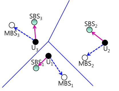
Figure 1: Example of double association. Each uplink device associates with one MBS and one SBS.

II System Model

We treat the scenario of a wireless heterogeneous network, composed of MBSs and SBSs, where each active user has an uplink (UL) transmission. The downlink (DL) transmission takes place in a time-frequency resource that is orthogonal to the one used for UL.

We assume that the MBSs and the SBSs are randomly located according to the 2-dimensional homogeneous Poisson point processes (PPP) $\Phi$ and $\Phi_{s}$ with node densities $\lambda$ and $\lambda_{s}$, respectively. The connection between the user and the MBS is assumed to use OFDMA-like orthogonal multiple access scheme, such that there is only one user per MBS using the same resource. To model this, the total area is considered as a Voronoi diagram, with the MBSs being the seeds of the diagram, such that each MBS defines one Voronoi cell. In each Voronoi cell one active UL user is deployed in a uniform random way across the cell area. Hence, the density of active UL users is also $\lambda$; however, the users are not generated by a Poisson point process, unlike the MBSs and SBSs. The distribution of users is a Poisson-Voronoi perturbed lattice [8] which is hard to analyze, but in order to make our analysis tractable, we will approximate it with a PPP with intensity $\lambda$. The tractability and accuracy of this approach has been demonstrated in [9]. The typical MBS is placed at the origin and the nearest user to the origin is the associated user. The nearest SBS to the user associated with the typical MBS is considered as the typical SBS. All performance figures are calculated for these two typical access points.

The double association is specified as follows. The $i-$th user associates with the MBS $M(i)$ deployed in the $i-$th Voronoi cell. Additionally, the $i-$th user’s transmission can reach the SBS $S(i)$ from which it receives the highest average power, i.e. the SBS that is closest geometrically:

$${S(i)}=\arg\mathop{\min}\limits_{j\in{\Phi_{s}}}r_{i,j},$$ (1)

where $r_{i,j}$ is the distance between the $i-$th active user and $j-$th SBS. The MBS acts as a primary access point, but the user transmission is simultaneously received by the MBS and the SBS. This scheme can be generalized to $k+1$ associations by having $k$ additional associations to the $k$ nearest SBSs, i.e. each user transmission has $k$ additional degrees of diversity.

All UL transmissions use the same spectrum and interfere with each other. The effects of path loss and fading are compensated by fractional power control (FPC) [10, 9]. The received signal strength at $B(i)$ from the $i-$th active user is:

$$G_{i,B(i)}r_{i,B(i)}^{-\alpha}\min(r_{i,M(i)}^{\alpha\epsilon}P,\bar{P}),$$ (2)

where $r_{i,B(i)}$ is the distance between the $i-$th active user and $B(i)\in\{M(i),S(i)\}$, $\alpha$ is the path-loss coefficient and $G_{i,B(i)}$ is an exponential random variable with unit mean in order to model the Rayleigh fading on the link. The time is slotted and the channel gain $G_{i,B(i)}$ is invariant in a slot. The transmit power is the minimum value between the maximum transmit power level constraint $\bar{P}$ and the power control component $r_{i,M(i)}^{\alpha\epsilon}P$, where $P$ is default transmit power level and $\epsilon$ is a power control factor (PCF) that can have values $0\!\leq\!\epsilon\!\leq\!1$. For $\epsilon\!=\!0$, no power control is applied, while $\epsilon\!=\!1$ corresponds to full channel inversion. The use of $r_{i,M(i)}$ indicates that power control is applied with respect to the distance to the associated MBS. Due to the dense deployment, we assume that the network is interference-limited and the effect of the noise is ignored. The success of the transmission is determined by the received signal-to-interference ratio (SIR) $\gamma_{B(i)}$ of the associated base station $B(i)\in\{M(i),S(i)\}$, given by:

$${\gamma_{B(i)}}\!\!=\!\!\frac{{{G_{i,B(i)}}r_{i,B(i)}^{-\alpha}\!\min(r_{i,M(i)}^{\alpha\epsilon},\!\bar{P})}}{{\sum\limits_{k\neq i}\!\!{{G_{k,B(i)}}r_{k,B(i)}^{-\alpha}\!\min(r_{k,M(k)}^{\alpha\epsilon},\!\bar{P})}}}\!\!=\!\!\frac{{{G_{i,B(i)}}r_{i,B(i)}^{-\alpha}\!\min(r_{i,M(i)}^{\alpha\epsilon},\!\bar{P})}}{I},$$ (3)

where $I$ denotes the aggregate interference. For a given target SIR threshold $\beta$, the transmission is successful if ${\gamma_{B(i)}}\geq\beta$. The data rate is a function of the target SIR following Shannon’s formula $\log_{2}\left(1\!+\!\beta\right)$ with a unit bandwidth. The transmit powers of the interfering users ($\min(r_{k,M(k)}^{\alpha\epsilon},\!\bar{P})$ in (3)) are actually not independent, since the area of the Voronoi cells of the adjacent users are correlated. In order to the analytical tractability, we will assume that the transmit powers of the interfering users are independent. The similar assumption is also made in [9].

As a reference scheme, the user $i$ associates with the one of the BSs (MBS or SBS), denoted by $j^{*}$, which has the maximal average received signal strength in the UL:

$${j^{*}}=\arg\mathop{\max}\limits_{j\in{\Phi_{b}}\cup{\Phi_{s}}}r_{i,j}^{-\alpha}P.$$ (4)

Note that the “classical” association is based on the received DL signal. Our reference scheme is thus related to the newly proposed DL/UL Decoupling (DUDe) [3], where the UL association is done according to (4) and is decoupled from the DL association. We call this scheme as a single association (SA). We use $p_{s}^{DA}$ to denote the success probability of DA. In the following sections, we analyze the success probability.

III Reliability Analysis of Double Association Scheme

Now we consider the success probability $p_{s}^{DA}$ of double association. The user connects to both the MBS and the SBS. Then the success probability is:

$${p_{s}^{DA}}=1-\Pr\left[{{\gamma_{M}}<\beta,{\gamma_{S}}<\beta}\right],$$ (5)

where $\gamma_{M}$ and $\gamma_{S}$ denote the received SIR at the typical MBS and SBS. Eq. (5) means the transmission is only failed if both MBS and SBS cannot receive the data. In our system model, MBSs and SBSs are deployed by independent point processes, such that these two probabilities are independent. We can rewrite (5) as follows:

$${p_{s}^{DA}}=1-\left({1-\Pr\left[{{\gamma_{M}}\geq\beta}\right]}\right)\left({1-\Pr\left[{{\gamma_{S}}\geq\beta}\right]}\right).$$ (6)

The probability $\Pr\left[{{\gamma_{M}}\geq\beta}\right]$ can be expressed as:

$$\Pr\left[{{\gamma_{M}}\geq\beta}\right]\! =\!\mathbb{E}_{r}\left[\Pr\left[{{\gamma_{M}}\geq\beta}|r\right]\right]$$

$$=\!\int_{0}^{\infty}\!\!\!{\Pr\left[{\frac{{G{r^{-\alpha}}{\min\left({{r^{\alpha\epsilon}}P,\bar{P}}\right)}}}{{{I_{M}}}}\!\geq\!\beta}\right]{f_{R}}\left(r\right)\!dr},$$ (7)

where $r$ denotes the distance to typical MBS. The FPC is performed based on the distance to the associated MBS. The term $I_{M}$ denotes the interference at typical MBS. The communication distance $r$ is a random variable with probability density function $f_{R}(r)$. As stated already, we approximate the user deployment process as PPP with intensity $\lambda$, such that the distance distribution becomes $f_{R}(r)={2\pi\lambda r{e^{-\pi\lambda{r^{2}}}}}$. The communication distances, which are the distances of the UL users to their associated MBSs, might be identically distributed, but not independent. The dependence is caused by the restriction that only one UL user can be situated in each Voronoi cell. This implies that, on average, the communication distances are closer compared to the communication distance in PPP since there is no restriction in PPP (See Fig. 2 in [9]). Hence, the success probability in PPP offers a lower bound to the original success probability, (III) expressed as follows:

$$\geq\!\int_{0}^{\infty}{\Pr\left[{\frac{{G{r^{-\alpha}}\min\left({{r^{\alpha\epsilon}}P,\bar{P}}\right)}}{{{I_{M}}}}\geq\beta}\right]2\pi\lambda r{e^{-\pi\lambda{r^{2}}}}dr}$$

$$\stackrel{{\scriptstyle(a)}}{{=}}\int_{0}^{\infty}{{\mathbb{E}_{{I_{M}}}}\left[{\exp\left({-\beta{r^{\alpha}}\min{{\left({{r^{\alpha\epsilon}}P,\bar{P}}\right)}^{-1}}{I_{M}}}\right)}\right]2\pi\lambda r{e^{-\pi\lambda{r^{2}}}}dr}$$

$$\stackrel{{\scriptstyle(b)}}{{=}}\int_{0}^{{{\hat{P}}^{\frac{1}{{\alpha\epsilon}}}}}{{\mathbb{E}_{{I_{M}}}}\left[{\exp\left({-\frac{{\beta{r^{\alpha}}{r^{-\alpha\epsilon}}}}{P}{I_{M}}}\right)}\right]2\pi\lambda r{e^{-\pi\lambda{r^{2}}}}dr}$$

$$\qquad\qquad+\int_{{{\hat{P}}^{\frac{1}{{\alpha\epsilon}}}}}^{\infty}{{\mathbb{E}_{{I_{M}}}}\left[{\exp\left({-\frac{{\beta{r^{\alpha}}}}{{\bar{P}}}{I_{M}}}\right)}\right]2\pi\lambda r{e^{-\pi\lambda{r^{2}}}}dr}$$

$$\stackrel{{\scriptstyle(c)}}{{=}}\!\!\int_{0}^{{{\hat{P}}^{\frac{1}{{\alpha\epsilon}}}}}\!\!{{{\cal L}_{{I_{M}}}}\left({{s_{1}}}\right)2\pi\lambda r{e^{-\pi\lambda{r^{2}}}}dr}\!+\!\int_{{{\hat{P}}^{\frac{1}{{\alpha\epsilon}}}}}^{\infty}\!\!{{{\cal L}_{{I_{M}}}}\left({{s_{2}}}\right)2\pi\lambda r{e^{-\pi\lambda{r^{2}}}}dr}$$ (8)

where (a) comes from the property of exponential random variable and takes the expectation of $I_{M}$. In (b), the integration is split into two parts, as the transmit power is varied with $r$ and $\bar{P}$ is selected when $r>{\hat{P}}^{\frac{1}{\alpha\epsilon}}$, where $\hat{P}=\bar{P}/P$. For (c), let us define ${s_{1}}={\beta{r^{\alpha}}{r^{-\alpha\epsilon}}}/P$ and ${s_{2}}={\beta{r^{\alpha}}}/{\bar{P}}$, then the expectation of $I_{M}$ becomes Laplace functional as follows:

$${{\mathcal{L}}_{{I_{M}}}}\left({{s_{1}}}\right) =\exp\Bigg{(}{-2\pi\lambda\int_{r}^{\infty}{\frac{{\beta{r^{\left({1-\epsilon}\right)\alpha}}{v^{-\alpha}}\hat{P}}}{{1+\beta{r^{\left({1-\epsilon}\right)\alpha}}{v^{-\alpha}}\hat{P}}}{e^{-\pi\lambda{{\hat{P}}^{\frac{2}{{\alpha\epsilon}}}}}}vdv}}-$$

$$2\pi \lambda\!\!\!\int_{r}^{\infty}\!\!\!\!\!{\int_{0}^{{{\hat{P}}^{\frac{1}{{\alpha\epsilon}}}}}\!\!\!\!\!\!\!{\frac{{\beta{r^{\left({1-\epsilon}\right)\alpha}}{v^{-\alpha}}{x^{\alpha\epsilon}}}}{{1\!\!+\!\beta{r^{\left({1-\epsilon}\right)\alpha}}{v^{-\alpha}}{x^{\alpha\epsilon}}}}2\pi\lambda x\exp\left({-\pi\lambda{x^{2}}}\right)\!vdxdv}}\Bigg{)}$$ (9)

$${{\mathcal{L}}_{{I_{M}}}}\left({{s_{2}}}\right) =\exp\Bigg{(}{-2\pi\lambda\int_{r}^{\infty}{\frac{{\beta{r^{\alpha}}{v^{-\alpha}}}}{{1+\beta{r^{\alpha}}{v^{-\alpha}}}}{e^{-\pi\lambda{{\hat{P}}^{\frac{2}{{\alpha\epsilon}}}}}}vdv}}-$$

$$2\pi \lambda\!\!\!\int_{r}^{\infty}\!\!\!\!\!{\int_{0}^{{{\hat{P}}^{\frac{1}{{\alpha\epsilon}}}}}\!\!\!\!\!\!\!{\frac{{\beta{r^{\alpha}}{v^{-\alpha}}{x^{\alpha\epsilon}}/\hat{P}}}{{1\!+\!\beta{r^{\alpha}}{v^{-\alpha}}{x^{\alpha\epsilon}}/\hat{P}}}2\pi\lambda x\!\exp\!\left({-\pi\lambda{x^{2}}}\right)\!vdx}dv}\Bigg{)}.$$ (10)

The derivation of (III) and (III) uses the property of PPP [7] and the integration of $v$ is made by using the distance from the interferers as a variable. The integration starts from $r$ due to the property of the Voronoi cells and no interferer can be closer to the typical MBS than the typical user associated with that MBS. The integration of $x$ uses the independent assumption of transmission powers of interferers and the integration range is limited to ${\hat{P}}^{\frac{1}{{\alpha\epsilon}}}$ for the same reason as (III)-(b).

The probability ${\Pr\left[{{\gamma_{S}}\geq\beta}\right]}$ can be obtained in a similar manner:

$$\Pr\left[{{\gamma_{S}}\geq\beta}\right] \!\simeq\!\int_{0}^{\infty}\Bigg{\{}\int_{0}^{{{\hat{P}}^{\frac{1}{{\alpha\epsilon}}}}}{{{\cal L}_{{I_{s}}}}\left({{s_{1}}}\right)2\pi\lambda r{e^{-\pi\lambda{r^{2}}}}dr}+$$

$$\qquad{{\cal L}_{{I_{s}}}}\left({{s_{2}}}\right){e^{-\pi\lambda{{\hat{P}}^{\frac{2}{{\alpha\epsilon}}}}}}\Bigg{\}}2\pi{\lambda_{s}}y{e^{-\pi{\lambda_{s}}{y^{2}}}}dy,$$ (11)

where ${s_{1}}=\frac{{\beta{y^{\alpha}}{r^{-\alpha\epsilon}}}}{P}$, ${s_{2}}=\frac{{\beta{y^{\alpha}}}}{{\bar{P}}}$, and $I_{S}$ denotes the interference at typical SBS. The Laplace functionals are

$${{\mathcal{L}}_{{I_{S}}}}\left({{s_{1}}}\right) =\exp\Bigg{(}{-2\pi\lambda\int_{0}^{\infty}{\frac{{\beta{y^{\alpha}}{r^{-\alpha\epsilon}}{u^{-\alpha}}\hat{P}}}{{1+\beta{y^{\alpha}}{r^{-\alpha\epsilon}}{u^{-\alpha}}\hat{P}}}{e^{-\pi\lambda{{\hat{P}}^{\frac{2}{{\alpha\epsilon}}}}}}udu}-}$$

$$2\pi\lambda \!\!\!\int_{0}^{\infty}\!\!\!\!\!{\int_{0}^{{{\hat{P}}^{\frac{1}{{\alpha\epsilon}}}}}\!\!\!\!\!\!\!{\frac{{\beta{y^{\alpha}}{r^{-\alpha\epsilon}}{u^{-\alpha}}{x^{\alpha\epsilon}}}}{{1\!+\!\beta{y^{\alpha}}{r^{-\alpha\epsilon}}{u^{-\alpha}}{x^{\alpha\epsilon}}}}\!2\pi\lambda x\!\exp\!\left({-\pi\lambda{x^{2}}}\right)\!udxdu}}\Bigg{)},$$ (12)

$${{\mathcal{L}}_{{I_{S}}}}\left({{s_{2}}}\right) =\!\exp\Bigg{(}{-2\pi\lambda\int_{0}^{\infty}{\frac{{\beta{y^{\alpha}}{u^{-\alpha}}}}{{1+\beta{y^{\alpha}}{u^{-\alpha}}}}{e^{-\pi\lambda{{\hat{P}}^{\frac{2}{{\alpha\epsilon}}}}}}udu}}-$$

$$2\pi\lambda\!\!\!\int_{0}^{\infty} \!\!\!\!\!{\int_{0}^{{{\hat{P}}^{\frac{1}{{\alpha\epsilon}}}}}\!\!\!\!\!\!\!\!{\frac{{\beta{y^{\alpha}}{u^{-\alpha}}{x^{\alpha\epsilon}}/\hat{P}}}{{1+\beta{y^{\alpha}}{u^{-\alpha}}{x^{\alpha\epsilon}}/\hat{P}}}2\pi\lambda x\exp\left({-\pi\lambda{x^{2}}}\right)udxdu}}\Bigg{)}.$$ (13)

For the SBSs, the distance of the interferers begins at zero since the interferer could be closer than the typical user. Using (III)-(III), the success probability (6) can be computed. Even though $p_{s}^{DA}$ is not a closed form, it can be easily computed numerically. With specific parameters $\alpha\!=\!4$ and $\epsilon\!=\!0$, a lower bound on $p_{s}^{DA}$ can be expressed in a closed form:

$${p_{s}^{DA}}\!\geq\!1\!-\!\left({1-\frac{1}{{1+\sqrt{\beta}\arctan\left({\sqrt{\beta}}\right)}}}\right)\left({1-\frac{{2{\lambda_{s}}}}{{\pi\sqrt{\beta}\lambda+2{\lambda_{s}}}}}\right).$$ (14)

IV Performance Evaluation

We use Monte Carlo simulation in order to assess the performance of the different association schemes and verify the analytical derivations. The node densities of MBSs and active uplink devices are set to $\lambda=0.01$, while the node density of SBSs is varied from $\lambda_{s}=0.02$ to $\lambda_{s}=0.05$. The path-loss exponent is $\alpha=4$ and the default transmit power for UL user is $P=30$dBm. The different PCF values $\epsilon=0,0.5,1$ and target thresholds $\beta=$0dB, 5dB are used.

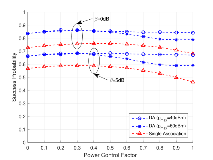
Figure 2: Success probability as a function of power control factor ($\lambda\!=\!0.01$, $\lambda_{s}\!=\!0.02$).

The transmission reliability is evaluated through the probability of success. Fig. 2 shows success probability as a function of power control factor ($\epsilon$). The reliability of DA is distinctly improved compared to that of SA. The lower target SINR threshold leads to a higher reliability performance, while, as expected, DA always outperforms SA. The small maximum power constraint (40dBm) will reduce the interference power and increase the reliability of DA compared to a higher constraint (60dBm). Even though utilizing lower PCF will increase the reliability, the effect of FPC is insignificant for DA. On the other hands, it is important to choose proper PCF for SA, as it is more sensitive and results in performance variation.

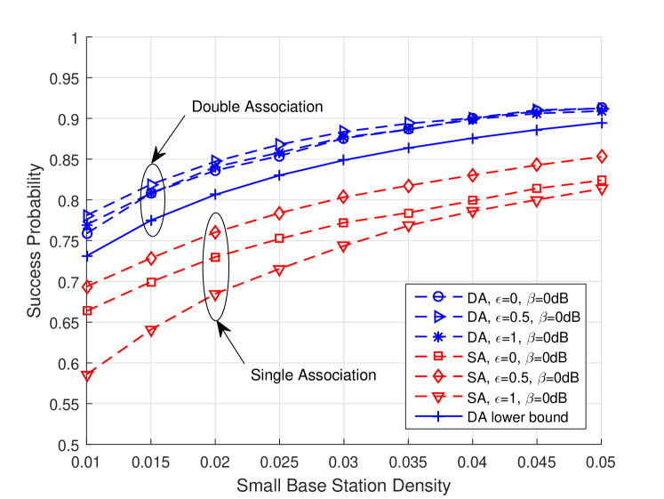
Figure 3: Success probability as a function of the small-cell base station density ($\lambda\!=\!0.01$, $\beta\!=\!0$ dB, $\bar{p}\!=\!50$ dBm).

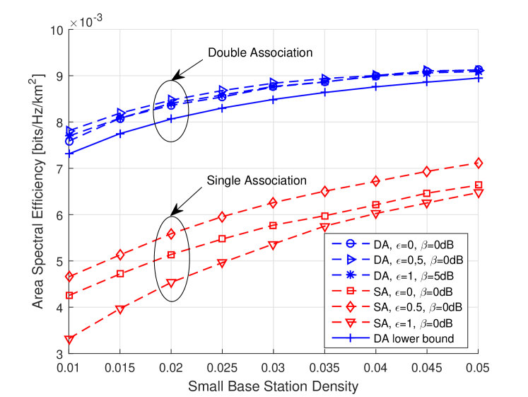
Figure 4: Area spectral efficiency as a function of the small-cell base station density ($\lambda\!=\!0.01$, $\beta\!=\!0$ dB, $\bar{p}\!=\!50$ dBm).

Fig. 3 shows the success probability as a function of the node density of SBSs. Already SA increases the success probability, but this is further increased by a double association. The analytical result shows a tight lower bound of the performance.

In order to assess the network throughput performance, we evaluate the area spectral efficiency, the product of the successfully transmitting user density and the data rate per node. Fig. 4 illustrates the area spectral efficiency as a function of the node density of SBSs. For the SBSs, multiple uplink users are connected to the same SBSs. Since the success of transmission is determined by the received SIR and the target threshold, only one user can succeed if the target threshold is $\beta\geq 1$. It can be seen that DA is superior to SA also in terms of area spectral efficiency.

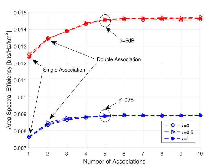
Figure 5: Area spectral efficiency as a function of the number of associations ($\lambda\!=\!0.01$, $\lambda_{s}\!=\!0.02$, $\beta\!=\!0$ dB, $\bar{p}\!=\!50$ dBm).

The derivation of the probabilities for $k\!+\!1$ associations is much more involved compared to the special case $k\!=\!1$ and requires elaboration that is outside the scope of this letter. Here we use simulation results to show how the reliability depends on $k$. By increasing the number of associations, the reliability of the transmission is improved, but rather saturated as the number of associations increase. The area spectral efficiency performance is depicted on Fig. 5. Increasing the number of associations is more favorable with as the target threshold increases. For example, having five associations is still beneficial for $\beta\!=\!5$dB, however, in case of $\beta\!=\!0$dB, the performance is almost saturated with three associations. Nevertheless, it can be seen clearly that the major performance increase comes when moving from single- to a double association.

V Concluding Remarks

We have considered methods for network association that improve the reliability of uplink transmissions in dense wireless heterogeneous networks. We have used stochastic geometry in order to analyze the performance of the schemes. The extensive simulation results show that double association, to one macro-cell Base Station (BS) and one small-cell BS, remarkably improves the probability of successful uplink transmission. As for the next steps, it is interesting to investigate the performance of a more complex method of processing the received data jointly across base stations. Finding the proper power control strategy is also interesting topic. If Successive Interference Cancellation (SIC) is applied along with double association, some of the uplink users can reduce the transmission power in order to catalyze the SIC process.

References

- [1] M. Z. Shafiq, L. Ji, A. X. Liu, J. Pang, and J. Wang, “Large-scale measurement and characterization of cellular machine-to-machine traffic,” IEEE/ACM Trans. Netw., vol. 21, no. 6, pp. 1960–1973, Dec. 2013.
- [2] A. Osseiran, V. Braun, T. Hidekazu, P. Marsch, H. Schotten, H. Tullberg, M. A. Uusitalo, and M. Schellman, “The foundation of the mobile and wireless communications system for 2020 and beyond: Challenges, enablers and technology solutions,” in Proc. IEEE VTC Spring 2013, Jun. 2013.
- [3] H. Elshaer, F. Boccardi, M. Dohler, and R. Irmer, “Downlink and uplink decoupling: a disruptive architectural design for 5G networks,” in Proc. IEEE GLOBECOM 2014, Dec. 2014.
- [4] K. Smiljkovikj, P. Popovski, and L. Gavrilovska, “Analysis of the decoupled access for downlink and uplink in wireless heterogeneous networks,” IEEE Wireless Commun. Lett., Apr. 2015.
- [5] D. Astely, E. Dahlman, G. Fodor, S. Parkvall, and J. Sachs, “LTE release 12 and beyond,” IEEE Commun. Mag., vol. 51, no. 7, pp. 154–160, Jul. 2013.
- [6] L. Falconetti and S. Landström, “Uplink coordinated multi-point reception in lte heterogeneous networks,” in Proc. ISWCS 2011, Nov. 2011.
- [7] D. Stoyan, W. Kendall, and J. Mecke, Stochastic Geometry and its Applications, 2nd ed. Wiley, 1995.
- [8] B. Błaszczyszyn and D. Yogeshwaran, “Clustering comparison of point processes, with applications to random geometric models,” in Stochastic Geometry, Spatial Statistics and Random Fields. Springer, 2015, pp. 31–71.
- [9] T. D. Novlan, H. S. Dhillon, and J. G. Andrews, “Analytical modeling of uplink cellular networks,” IEEE Trans. Wireless Commun., vol. 12, no. 6, pp. 2669–2679, Jun. 2013.
- [10] C. U. Castellanos, D. L. Villa, C. Rosa, K. Pedersen, F. D. Calabrese, P.-H. Michaelsen, and J. Michel, “Performance of uplink fractional power control in UTRAN LTE,” in Proc. IEEE VTC Spring 2008, May 2008.
- [11] G. Nigam, P. Minero, and M. Haenggi, “Coordinated multipoint joint transmission in heterogeneous networks,” IEEE Trans. Commun., vol. 62, no. 11, pp. 4134–4146, Nov. 2014.
- [12] F. Baccelli and A. Giovanidis, “A stochastic geometry framework for analyzing pairwise-cooperative cellular networks,” IEEE Trans. Wireless Commun., vol. 14, no. 2, pp. 794–808, Feb. 2015.