A new generalization of the $P_{1}$ non-conforming FEM to higher polynomial degrees

Abstract

This paper generalizes the non-conforming FEM of Crouzeix and Raviart and its fundamental projection property by a novel mixed formulation for the Poisson problem based on the Helmholtz decomposition. The new formulation allows for ansatz spaces of arbitrary polynomial degree and its discretization coincides with the mentioned non-conforming FEM for the lowest polynomial degree. The discretization directly approximates the gradient of the solution instead of the solution itself. Besides the a priori and medius analysis, this paper proves optimal convergence rates for an adaptive algorithm for the new discretization. These are also demonstrated in numerical experiments. Furthermore, this paper focuses on extensions of this new scheme to quadrilateral meshes, mixed FEMs, and three space dimensions.

Keywords non-conforming FEM, Helmholtz decomposition, mixed FEM, adaptive FEM, optimality

AMS subject classification 65N30, 65N12, 65N15

1 Introduction

Non-conforming finite element methods (FEMs) play an important role in computational mechanics. They allow the discretization of partial differential equations (PDEs) for incompressible fluid flows, for almost incompressible materials in linear elasticity, and for low polynomial degrees in the ansatz spaces for higher-order problems. The projection property of the interpolation operator of the $P_{1}$ non-conforming FEM, also named after Crouzeix and Raviart [21], states that the $L^{2}$ projection of $\nabla H^{1}_{0}(\Omega)$ onto the space of piecewise constant functions equals the space of piecewise gradients of the non-conforming interpolation of $H^{1}_{0}(\Omega)$ functions in the $P_{1}$ non-conforming finite element space. This property is the basis for the proof of the discrete inf-sup condition for the Stokes equations [21] as well as for the analysis of adaptive algorithms [6].

Many possible generalizations of the $P_{1}$ non-conforming FEM to higher polynomial degrees have been proposed. All those generalizations are either based on a modification of the classical concept of degrees of freedom [23, 22, 41], are restricted to odd polynomial degrees [20, 3], or employ an enrichment by additional bubble-functions [29, 28]. However, none of those generalizations possesses a corresponding projection property of the interpolation operator for higher moments (see Remark 3.15 below). This paper introduces a novel formulation of the Poisson equation (in (3.3) below) based on the Helmholtz decomposition along with its discretization of arbitrary (globally fixed) polynomial degree. This new discretization approximates directly the gradient of the solution, which is often the quantity of interest, instead of the solution itself. For the lowest-order polynomial degree, the discrete Helmholtz decomposition of [4] proves equivalence of the novel discretization with the known non-conforming Crouzeix-Raviart FEM [21] and therefore they appear in a natural hierarchy. In the context of the novel (mixed) formulation, these discretizations turn out to be conforming. Although the complexity of the new discretization itself is competitive with that of a standard FEM, the method requires the pre-computation of some function $\varphi$ such that its divergence equals the right-hand side. If this is not computable analytically, this results in an additional integration (see also Remark 3.6 below). However, this paper focuses on the Poisson problem as a model problem to introduce the idea of the new approach and to give a broad impression over possible extensions as quadrilateral discretizations (including a discrete Helmholtz decomposition on quadrilateral meshes for the non-conforming Rannacher-Turek FEM [33] as a further highlight of this paper), the generalization to three dimensions, or inhomogeneous mixed boundary conditions. The advantages of the new approach in some applications will be the topic of forthcoming papers [36, 37].

The presence of singularities for non-convex domains usually yields the same sub-optimal convergence rate for any polynomial degree. This motivates adaptive mesh-generation strategies, which recover the optimal convergence rates. This paper presents an adaptive algorithm and proves its optimal convergence. The proof essentially follows ideas from the context of the non-conforming Crouzeix-Raviart FEM [6, 32]. This illustrates that the novel discretization generalizes it in a natural way. Since the efficient and reliable error estimator involves a data approximation term without a multiplicative power of the mesh-size, the adaptive algorithm is based on separate marking.

A possible drawback of the new FEMs is that the gradient of the solution $\nabla u$ is approximated, but not the solution $u$ itself. This excludes obvious generalizations to partial differential equations where $u$ appears in lower-order terms.

The remaining parts of this paper are organized as follows. Section 2 defines some notation. Section 3 introduces the novel formulation based on the Helmholtz decomposition and its discretization together with an a priori error estimate. The equivalence with the $P_{1}$ non-conforming FEM for the lowest-order case is proved in Subsection 3.3. Section 4 summarizes some generalizations. Section 5 is devoted to a medius analysis of the FEM, which uses a posteriori techniques to derive a priori error estimates. Section 6 proves quasi-optimality of an adaptive algorithm, while Section 7 outlines the generalization to 3D. Section 8 concludes this paper with numerical experiments.

2 Notation

Throughout this paper $\Omega\subseteq\mathbb{R}^{2}$ is a simply connected, bounded, polygonal Lipschitz domain. Standard notation on Lebesgue and Sobolev spaces and their norms is employed with $L^{2}$ scalar product $(\bullet,\bullet)_{L^{2}(\Omega)}$. Given a Hilbert space $X$, let $L^{2}(\Omega;X)$ resp. $H^{k}(\Omega;X)$ denote the space of functions with values in $X$ whose components are in $L^{2}(\Omega)$ resp. $H^{k}(\Omega)$ and let $L^{2}_{0}(\Omega)$ denote the subset of $L^{2}(\Omega)$ of functions with vanishing integral mean. The space of $L^{2}$ functions whose weak divergence exists and is in $L^{2}$ is denoted with $H(\operatorname{div},\Omega)$. The space of infinitely differentiable functions reads $C^{\infty}(\Omega)$ and the subspace of functions with compact support in $\Omega$ is denoted with $C^{\infty}_{c}(\Omega)$. The piecewise action of differential operators is denoted with a subscript ​N​C. The formula $A\lesssim B$ represents an inequality $A\leq CB$ for some mesh-size independent, positive generic constant $C$; $A\approx B$ abbreviates $A\lesssim B\lesssim A$. By convention, all generic constants $C\approx 1$ do neither depend on the mesh-size nor on the level of a triangulation but may depend on the fixed coarse triangulation $\mathcal{T}_{0}$ and its interior angles. The Curl operator in two dimensions is defined by $\operatorname{Curl}\beta:=(\partial\beta/\partial x_{2},-\partial\beta/\partial x_{1})$ for sufficiently smooth $\beta$.

A shape-regular triangulation $\mathcal{T}$ of a bounded, polygonal, open Lipschitz domain $\Omega\subseteq\mathbb{R}^{2}$ is a set of closed triangles $T\in\mathcal{T}$ such that $\overline{\Omega}=\bigcup\mathcal{T}$ and any two distinct triangles are either disjoint or share exactly one common edge or one vertex. Let $\mathcal{E}(T)$ denote the edges of a triangle $T$ and $\mathcal{E}:=\mathcal{E}(\mathcal{T}):=\bigcup_{T\in\mathcal{T}}\mathcal{E}(T)$ the set of edges in $\mathcal{T}$. Any edge $E\in\mathcal{E}$ is associated with a fixed orientation of the unit normal $\nu_{E}$ on $E$ (and $\tau_{E}=(0,-1;1,0)\nu_{E}$ denotes the unit tangent on $E$). On the boundary, $\nu_{E}$ is the outer unit normal of $\Omega$, while for interior edges $E\not\subseteq\partial\Omega$, the orientation is fixed through the choice of the triangles $T_{+}\in\mathcal{T}$ and $T_{-}\in\mathcal{T}$ with $E=T_{+}\cap T_{-}$ and $\nu_{E}:=\nu_{T_{+}}|_{E}$ is then the outer normal of $T_{+}$ on $E$. In this situation, $[v]_{E}:=v|_{T_{+}}-v|_{T_{-}}$ denotes the jump across $E$. For an edge $E\subseteq\partial\Omega$ on the boundary, the jump across $E$ reads $[v]_{E}:=v$. For $T\in\mathcal{T}$ and $X\subseteq\mathbb{R}^{n}$, let

$$P_{k}(T;X) :=\left\{v:T\rightarrow X\left|\begin{array}[]{l}\text{each component}\text{ of }v\text{ is a polynomial}\\ \text{of total degree}\leq k\end{array}\right\}\right.;$$

$$P_{k}(\mathcal{T};X) :=\{v:\Omega\rightarrow X\;|\;\forall T\in\mathcal{T}:\;v|_{T}\in P_{k}(T;X)\}$$

denote the set of piecewise polynomials and $P_{k}(\mathcal{T}):=P_{k}(\mathcal{T};\mathbb{R})$. Given a subspace $X\subseteq L^{2}(\Omega;\mathbb{R}^{n})$, let $\Pi_{X}:L^{2}(\Omega;\mathbb{R}^{n})\to X$ denote the $L^{2}$ projection onto $X$ and let $\Pi_{k}$ abbreviate $\Pi_{P_{k}(\mathcal{T};\mathbb{R}^{n})}$. Given a triangle $T\in\mathcal{T}$, let $h_{T}:=(\mathrm{meas}_{2}(T))^{1/2}$ denote the square root of the area of $T$ and let $h_{\mathcal{T}}\in P_{0}(\mathcal{T})$ denote the piecewise constant mesh-size with $h_{\mathcal{T}}|_{T}:=h_{T}$ for all $T\in\mathcal{T}$. For a set of triangles $\mathcal{M}\subseteq\mathcal{T}$, let $\|\bullet\|_{\mathcal{M}}$ abbreviate

$$\|\bullet\|_{\mathcal{M}}:=\sqrt{\sum_{T\in\mathcal{M}}\|\bullet\|_{L^{2}(T)}^{2}}.$$

Given an initial triangulation $\mathcal{T}_{0}$, an admissible triangulation is a regular triangulation which can be created from $\mathcal{T}_{0}$ by newest-vertex bisection [40]. The set of admissible triangulations is denoted by $\mathbb{T}$.

3 Problem formulation and discretization

This section introduces the new formulation based on the Helmholtz decomposition in Subsection 3.1 and its discretization in Subsection 3.2. Subsection 3.3 discusses the equivalence with the $P_{1}$ non-conforming Crouzeix-Raviart FEM [21].

3.1 New mixed formulation of the Poisson problem

Given the simply connected, bounded, polygonal Lipschitz domain $\Omega\subseteq\mathbb{R}^{2}$ and $f\in L^{2}(\Omega)$, the Poisson model problem seeks $u\in H^{1}_{0}(\Omega)$ with

$$-\Delta u=f\text{ in }\Omega\qquad\text{and}\qquad u=0\text{ on }\partial\Omega.$$ (3.1)

The novel weak formulation is based on the classical Helmholtz decomposition [35]

$$L^{2}(\Omega;\mathbb{R}^{2})=\nabla H^{1}_{0}(\Omega)\oplus\operatorname{Curl}(H^{1}(\Omega)\cap L^{2}_{0}(\Omega))$$ (3.2)

for any simply connected domain $\Omega\subseteq\mathbb{R}^{2}$, where the sum is orthogonal with respect to the $L^{2}$ scalar product.

Remark 3.1.

Note that for $\Omega\subseteq\mathbb{R}^{2}$, the definition of the Curl implies

$$H(\operatorname{Curl},\Omega):=\{\beta\in L^{2}(\Omega)\mid\operatorname{Curl}\beta\in L^{2}(\Omega)\}=H^{1}(\Omega).$$

Define $X:=L^{2}(\Omega;\mathbb{R}^{2})$ and $Y:=H^{1}(\Omega)\cap L^{2}_{0}(\Omega)$ and let $\varphi\in H(\operatorname{div},\Omega)$ satisfy $-\operatorname{div}\varphi=f$. The novel weak formulation of the Poisson problem (3.1) seeks $(p,\alpha)\in X\times Y$ with

$$(p,q)_{L^{2}(\Omega)}+(q,\operatorname{Curl}\alpha)_{L^{2}(\Omega)} =(\varphi,q)_{L^{2}(\Omega)} \text{ for all }q\in X,$$ (3.3)

$$(p,\operatorname{Curl}\beta)_{L^{2}(\Omega)} =0 \text{ for all }\beta\in Y.$$

This formulation is the point of departure for the numerical approximation of $\nabla u$ in Subsection 3.2.

Remark 3.2 (existence of solutions).

Since $\operatorname{Curl}Y\subseteq X$, any $\beta\in Y$ satisfies the inf-sup condition

$$\left\|\operatorname{Curl}\beta\right\|_{L^{2}(\Omega)}\leq\sup_{q\in X\setminus\{0\}}\frac{(q,\operatorname{Curl}\beta)_{L^{2}(\Omega)}}{\|q\|_{L^{2}(\Omega)}}.$$

This and Brezzi’s splitting lemma [11] imply the unique existence of a solution $(p,\alpha)\in X\times Y$ to (3.3). The $L^{2}$ orthogonality of $p$ and $\operatorname{Curl}\alpha$ implies

$$\|p\|_{L^{2}(\Omega)}^{2}+\left\|\operatorname{Curl}\alpha\right\|_{L^{2}(\Omega)}^{2}=\|\varphi\|_{L^{2}(\Omega)}^{2}.$$

Remark 3.3 (equivalence of (3.1) and (3.3)).

The second equation of (3.3) and the Helmholtz decomposition (3.2) imply the existence of $\widetilde{u}\in H^{1}_{0}(\Omega)$ with $p=\nabla\widetilde{u}$. Since $\varphi\in H(\operatorname{div},\Omega)$ satisfies $-\operatorname{div}\varphi=f$, the $L^{2}$ orthogonality in (3.2) implies that any $v\in H^{1}_{0}(\Omega)$ satisfies

$$(p,\nabla v)_{L^{2}(\Omega)}=(\varphi,\nabla v)_{L^{2}(\Omega)}=(f,v)_{L^{2}(\Omega)}$$

and, hence, $\widetilde{u}$ solves (3.1).

Remark 3.4 (mixed boundary conditions).

Let $\partial\Omega=\Gamma_{D}\cup\Gamma_{N}$ with $\Gamma_{D}$ closed, $\Gamma_{D}\cap\Gamma_{N}=\emptyset$, and each connectivity component of $\Gamma_{D}$ has positive length. Assume that the triangulation resolves $\Gamma_{D}$. Let $H^{-1/2}(\Gamma_{N})$ denote the space of generalized normal traces of $H(\operatorname{div},\Omega)$ functions and let $u_{D}\in H^{1}(\Omega)$ and $g\in H^{-1/2}(\Gamma_{N})$ in the sense that there holds $g=q\cdot\nu$ on $\Gamma_{N}$ in the sense of distributions for some $q\in H(\operatorname{div},\Omega)$. Consider the mixed boundary value problem $-\Delta u=f$ in $\Omega$ with $u|_{\Gamma_{D}}=u_{D}$ on $\Gamma_{D}$ and $(\nabla u\cdot\nu)|_{\Gamma_{N}}=g$ on $\Gamma_{N}$. Let $H^{1}_{D}(\Omega)$ denote the subspace of $H^{1}(\Omega)$ of functions with vanishing trace on $\Gamma_{D}$. For $\Gamma_{D}=\emptyset$, define $H^{1}_{D}(\Omega):=H^{1}(\Omega)\cap L^{2}_{0}(\Omega)$. Define

$$H^{1}_{\star}(\Omega) :=\{\beta\in Y\mid\beta\text{ is constant on each connectivity component of }\Gamma_{N}\}.$$

The Helmholtz decomposition

$$L^{2}(\Omega;\mathbb{R}^{2})=\nabla H^{1}_{D}(\Omega)\oplus\operatorname{Curl}H^{1}_{\star}(\Omega)$$

for mixed boundary conditions [24, Corollary 3.1] then leads to the following formulation. Let $\varphi\in H(\operatorname{div},\Omega)$ with $-\operatorname{div}\varphi=f$ additionally fulfil the boundary condition $\varphi\nu|_{\Gamma_{N}}=g$ and seek $(p,\alpha)\in L^{2}(\Omega;\mathbb{R}^{2})\times H^{1}_{\star}(\Omega)$ with

$$(p,q)_{L^{2}(\Omega)}+(q,\operatorname{Curl}\alpha)_{L^{2}(\Omega)} =(\varphi,q)_{L^{2}(\Omega)} \text{ for all }q\in L^{2}(\Omega;\mathbb{R}^{2}),$$

$$(p,\operatorname{Curl}\beta)_{L^{2}(\Omega)} =(\nabla u_{D},\operatorname{Curl}\beta)_{L^{2}(\Omega)} \text{ for all }\beta\in H^{1}_{\star}(\Omega).$$

Since $p=\varphi-\operatorname{Curl}\alpha\in H(\operatorname{div},\Omega)$, the equivalence follows as in Subsection 3.1 and with

$$(p\cdot\nu)|_{\Gamma_{N}}=(\varphi\cdot\nu)|_{\Gamma_{N}}-(\operatorname{Curl}\alpha\cdot\nu)|_{\Gamma_{N}}=g-(\nabla\alpha\cdot\tau)|_{\Gamma_{N}}=g.$$

Remark 3.5 (multiply connected domains).

If $\Omega\subseteq\mathbb{R}^{2}$ is a multiply connected polygonal bounded Lipschitz domain and $\partial\Omega=\Gamma_{D}\cup\Gamma_{N}$, such that all parts of $\Gamma_{D}$ lie on the outer boundary of $\Omega$ (on the unbounded connectivity component of $\mathbb{R}^{2}\setminus\Omega$), then the Helmholtz decomposition of Remark 3.4 still holds and a discretization as above is then immediate. However, if the Dirichlet boundary $\Gamma_{D}$ also covers parts of interior boundary, that Helmholtz decomposition does no longer hold: There exist harmonic functions which are constant on different parts of $\Gamma_{D}$ and, hence, are neither in $\nabla H^{1}_{\Gamma_{D}}(\Omega)$, nor in $\operatorname{Curl}H^{1}_{\star}(\Omega)$.

Remark 3.6 (computation of $\varphi$).

The computation of $\varphi$ appears as a practical difficulty because $\varphi$ needs to be defined through an integration of $f$. If $f$ has some simple structure, e.g., $f$ is polynomial, this can be done manually, while for more complicated $f$, a numerical integration of $f$ has to be employed, but is possible in parallel.

3.2 Discretization

Let $\mathcal{T}$ be a regular triangulation of $\Omega$ and $k\in\mathbb{N}\cup\{0\}$ and define

$$X_{h}(\mathcal{T}):=P_{k}(\mathcal{T};\mathbb{R}^{2})\quad\text{and}\quad Y_{h}(\mathcal{T}):=P_{k+1}(\mathcal{T})\cap Y.$$

The discretization of (3.3) seeks $p_{h}\in X_{h}(\mathcal{T})$ and $\alpha_{h}\in Y_{h}(\mathcal{T})$ with

$$(p_{h},q_{h})_{L^{2}(\Omega)}+(q_{h},\operatorname{Curl}\alpha_{h})_{L^{2}(\Omega)} =(\varphi,q_{h})_{L^{2}(\Omega)} \text{ for all }q_{h}\in X_{h}(\mathcal{T}),$$ (3.4.a)

$$(p_{h},\operatorname{Curl}\beta_{h})_{L^{2}(\Omega)} =0 \text{ for all }\beta_{h}\in Y_{h}(\mathcal{T}).$$ (3.4.b)

Remark 3.7.

Since there are no continuity conditions on $q_{h}\in X_{h}(\mathcal{T})$ and since $\operatorname{Curl}Y_{h}(\mathcal{T})\subseteq X_{h}(\mathcal{T})$, the first equation is fulfilled in a strong form, i.e.,

$$p_{h}+\operatorname{Curl}\alpha_{h}=\Pi_{k}\varphi.$$

In contrast to classical finite element methods, the approximation $p_{h}$ of $\nabla u$ is a gradient only in a discrete orthogonal sense, namely (3.4.b). For $k=0$, Subsection 3.3 below proves that this discrete orthogonal gradient property is equivalent to being a non-conforming gradient of a Crouzeix-Raviart finite element function. The main motivation of the novel formulation is the generalization of this scheme to any polynomial degree $k$.

Remark 3.8 (existence of discrete solutions).

Since $\operatorname{Curl}Y_{h}(\mathcal{T})\subseteq X_{h}(\mathcal{T})$, the discrete inf-sup condition

$$\left\|\operatorname{Curl}\beta_{h}\right\|_{L^{2}(\Omega)}\leq\sup_{q_{h}\in X_{h}(\mathcal{T})\setminus\{0\}}\frac{(q_{h},\operatorname{Curl}\beta_{h})_{L^{2}(\Omega)}}{\|q_{h}\|_{L^{2}(\Omega)}}\qquad\text{for all }\beta_{h}\in Y_{h}(\mathcal{T})$$

is fulfilled. This and Brezzi’s splitting lemma [11] imply the unique existence of a solution $(p_{h},\alpha_{h})\in X_{h}(\mathcal{T})\times Y_{h}(\mathcal{T})$ to (3.4). The equality in

$$\|p_{h}\|_{L^{2}(\Omega)}^{2}+\left\|\operatorname{Curl}\alpha_{h}\right\|_{L^{2}(\Omega)}^{2}=\|\Pi_{k}\varphi\|_{L^{2}(\Omega)}^{2}\leq\|\varphi\|_{L^{2}(\Omega)}^{2}.$$

follows from the $L^{2}$ orthogonality of $p_{h}$ and $\operatorname{Curl}\alpha_{h}$.

The conformity of the method and the inf-sup conditions from Remarks 3.2 and 3.8 imply the following best-approximation result.

Theorem 3.9 (best-approximation).

The solution $(p,\alpha)\in X\times Y$ to (3.3) and the discrete solution $(p_{h},\alpha_{h})\in X_{h}(\mathcal{T})\times Y_{h}(\mathcal{T})$ of (3.4) satisfy

$$\|p-p_{h}\|_{L^{2}(\Omega)}+\left\|\operatorname{Curl}(\alpha-\alpha_{h})\right\|_{L^{2}(\Omega)}$$ (3.5)

$$\qquad\qquad\lesssim\Big{(}\min_{q_{h}\in X_{h}(\mathcal{T})}\|p-q_{h}\|_{L^{2}(\Omega)}+\min_{\beta_{h}\in Y_{h}(\mathcal{T})}\left\|\operatorname{Curl}(\alpha-\beta_{h})\right\|_{L^{2}(\Omega)}\Big{)}.$$ ∎

Remark 3.10.

A direct analysis of the bilinear form $\mathcal{B}:\big{(}X\times Y\big{)}\times\big{(}X\times Y\big{)}\to\mathbb{R}$ defined by

$$\mathcal{B}((p,\alpha),(q,\beta)):=(p,q)_{L^{2}(\Omega)}+(q,\operatorname{Curl}\alpha)_{L^{2}(\Omega)}+(p,\operatorname{Curl}\beta)_{L^{2}(\Omega)}$$ (3.6)

for all $p,q\in X$ and all $\alpha,\beta\in Y$ reveals that the inf-sup constant of $\mathcal{B}$ equals $5$ and, hence, the constant hidden in $\lesssim$ in (3.5) is $5$.

Remark 3.11.

The best-approximation of Theorem 3.9 contains the term

$$\min_{\beta_{h}\in Y_{h}(\mathcal{T})}\left\|\operatorname{Curl}(\alpha-\beta_{h})\right\|_{L^{2}(\Omega)}$$

on the right-hand side, which depends on the choice of $\varphi$. This seems to be worse than the best-approximation results for standard FEMs, which do not involve such a term. However, if $\varphi$ is chosen smooth enough, then $\operatorname{Curl}\alpha=\varphi-\nabla u$ has at least the same regularity as $\nabla u$, and therefore the convergence rate is not diminished. On the other hand, the approximation space for $p$ does not have any continuity restriction and so the first approximation term

$$\min_{q_{h}\in X_{h}(\mathcal{T})}\|p-q_{h}\|_{L^{2}(\Omega)}$$ (3.7)

is superior to the best-approximation of a standard FEM, where $p=\nabla u$ is approximated with gradients of finite element functions. However, [42, Theorem 3.2] and the comparison results of [15] prove equivalence of (3.7) and the best-approximation with gradients of a standard FEM up to some multiplicative constant.

The following lemma proves a projection property. This means that for any $v\in H^{1}_{0}(\Omega)$, the best-approximation of $\nabla v$ in $X_{h}(\mathcal{T})$ is a discrete orthogonal gradient in the sense that it is orthogonal to $\operatorname{Curl}Y_{h}(\mathcal{T})$ and so belongs to the set of discrete orthogonal gradients $W_{h}(\mathcal{T})$ defined by

$$W_{h}(\mathcal{T}):=\{q_{h}\in X_{h}(\mathcal{T})\mid(q_{h},\operatorname{Curl}\beta_{h})_{L^{2}(\Omega)}=0\text{ for all }\beta_{h}\in Y_{h}(\mathcal{T})\}.$$ (3.8)

The projection property is the key ingredient in the optimality analysis of Section 6.

Lemma 3.12 (projection property).

It holds that $W_{h}(\mathcal{T})=\Pi_{X_{h}(\mathcal{T})}\nabla H^{1}_{0}(\Omega)$. Moreover, if $\mathcal{T}_{\star}$ is an admissible refinement of $\mathcal{T}$, then $\Pi_{X_{h}(\mathcal{T})}W_{h}(\mathcal{T}_{\star})=W_{h}(\mathcal{T})$.

Proof.

Let $q\in\nabla H^{1}_{0}(\Omega)$. Since $\operatorname{Curl}Y_{h}(\mathcal{T})\subseteq X_{h}(\mathcal{T})$ and $Y_{h}(\mathcal{T})\subseteq Y$, the orthogonality in the Helmholtz decomposition (3.2) implies for any $\beta_{h}\in Y_{h}(\mathcal{T})$ that

$$(\Pi_{X_{h}(\mathcal{T})}q,\operatorname{Curl}\beta_{h})_{L^{2}(\Omega)}=(q,\operatorname{Curl}\beta_{h})_{L^{2}(\Omega)}=0.$$

This proves $\Pi_{X_{h}(\mathcal{T})}\nabla H^{1}_{0}(\Omega)\subseteq W_{h}(\mathcal{T})$. For the converse direction, let $p_{h}\in W_{h}(\mathcal{T})$ and let $u\in H^{1}_{0}(\Omega)$ be a solution (possibly not unique) to

$$(\Pi_{X_{h}(\mathcal{T})}\nabla u,\Pi_{X_{h}(\mathcal{T})}\nabla v)_{L^{2}(\Omega)}=(p_{h},\Pi_{X_{h}(\mathcal{T})}\nabla v)_{L^{2}(\Omega)}\qquad\text{for all }v\in H^{1}_{0}(\Omega).$$

The orthogonality of $p_{h}-\Pi_{X_{h}(\mathcal{T})}\nabla u$ to $\nabla H^{1}_{0}(\Omega)$ implies the existence of $\alpha\in Y$ such that $p_{h}-\Pi_{X_{h}(\mathcal{T})}\nabla u=\operatorname{Curl}\alpha$. Therefore, $\operatorname{Curl}\alpha\in X_{h}(\mathcal{T})$ and, hence, $\alpha$ is a piecewise polynomial of degree $\leq k+1$ and therefore $\alpha\in Y_{h}(\mathcal{T})$. But since $p_{h}\in W_{h}(\mathcal{T})$, it holds that

$$\left\|\operatorname{Curl}\alpha\right\|_{L^{2}(\Omega)}^{2}=(p_{h}-\Pi_{X_{h}(\mathcal{T})}\nabla u,\operatorname{Curl}\alpha)_{L^{2}(\Omega)}=0$$

and, hence, $\alpha=0$. This proves $\Pi_{X_{h}(\mathcal{T})}\nabla u=p_{h}$ and, therefore, $W_{h}(\mathcal{T})\subseteq\Pi_{X_{h}(\mathcal{T})}\nabla H^{1}_{0}(\Omega)$.

A similar proof applies in the discrete case and proves $\Pi_{X_{h}(\mathcal{T})}W_{h}(\mathcal{T}_{\star}=W_{h}(\mathcal{T})$. ∎

Remark 3.13 (computational costs).

Problem (3.4) is equivalent to the problem: Find $(p_{h},\alpha_{h})\in X_{h}(\mathcal{T})\times Y_{h}(\mathcal{T})$ such that

$$(\operatorname{Curl}\beta_{h},\operatorname{Curl}\alpha_{h})_{L^{2}(\Omega)} =(\varphi,\operatorname{Curl}\beta_{h})_{L^{2}(\Omega)}\qquad\text{for all }\beta_{h}\in Y_{h}(\mathcal{T}),$$

$$p_{h} =\Pi_{X_{h}(\mathcal{T})}\varphi-\operatorname{Curl}\alpha_{h}.$$

Therefore, the system matrix is (in 2D) the same than that of a standard FEM (up to degrees of freedom on the boundary).

3.3 Equivalence with Crouzeix-Raviart FEM

The non-conforming Crouzeix-Raviart finite element space [21] reads

$$\mathrm{CR}^{1}_{0}(\mathcal{T}):=\left\{v_{\mathrm{CR}}\in P_{1}(\mathcal{T})\left|\begin{array}[]{l}v_{\mathrm{CR}}\text{ is continuous at midpoints of interior edges}\\ \text{and vanishes at midpoints of boundary edges}\end{array}\right\}\right..$$

Since $\mathrm{CR}^{1}_{0}(\mathcal{T})\not\subseteq H^{1}_{0}(\Omega)$ (if the triangulation consists of more than one triangle), the weak gradient of a function $v_{\mathrm{CR}}\in\mathrm{CR}^{1}_{0}(\mathcal{T})$ does not exist in general. However, the piecewise version $\nabla_{\text{\!\tiny\rm N\!C}}v_{\mathrm{CR}}\in P_{0}(\mathcal{T};\mathbb{R}^{2})$ defined by $(\nabla_{\text{\!\tiny\rm N\!C}}v_{\mathrm{CR}})|_{T}:=\nabla(v_{\mathrm{CR}}|_{T})$ for all $T\in\mathcal{T}$ exists. The $P_{1}$ non-conforming discretization of the Poisson problem seeks $u_{\mathrm{CR}}\in\mathrm{CR}^{1}_{0}(\mathcal{T})$ with

$$(\nabla_{\text{\!\tiny\rm N\!C}}u_{\mathrm{CR}},\nabla_{\text{\!\tiny\rm N\!C}}v_{\mathrm{CR}})_{L^{2}(\Omega)}=(f,v_{\mathrm{CR}})_{L^{2}(\Omega)}\qquad\text{for all }v_{\mathrm{CR}}\in\mathrm{CR}^{1}_{0}(\mathcal{T}).$$ (3.9)

The lowest-order space of Raviart-Thomas finite element functions [34] reads

$$\mathrm{RT}_{0}(\mathcal{T}):=\left\{q_{\mathrm{RT}}\in H(\operatorname{div},\Omega)\left|\begin{array}[]{l}\forall T\in\mathcal{T}\,\exists a_{T}\in\mathbb{R}^{2},b_{T}\in\mathbb{R}\\ \text{with }q_{\mathrm{RT}}(x)=a_{T}+b_{T}x\end{array}\right\}\right..$$ (3.12)

The Raviart-Thomas functions have the property that the integration by parts formula holds for functions in $H^{1}_{0}(\Omega)$ as well as for functions in $\mathrm{CR}^{1}_{0}(\mathcal{T})$.

The following proposition proves the equivalence of the $P_{1}$ non-conforming discretization and the discretization (3.4) for $k=0$. Note that the discretization (3.9) is a non-conforming discretization, while the discretization (3.4) is a conforming one.

Proposition 3.14 (equivalence with CR-NCFEM).

Let $f\in P_{0}(\mathcal{T})$ be piecewise constant and let $\varphi_{\mathrm{RT}}\in\mathrm{RT}_{0}(\mathcal{T})$ satisfy $-\operatorname{div}\varphi_{\mathrm{RT}}=f$. Then the discrete solution $(p_{h},\alpha_{h})\in P_{0}(\mathcal{T};\mathbb{R}^{2})\times(P_{1}(\mathcal{T})\cap Y)$ to (3.4) for $k=0$ and the gradient of the discrete solution $u_{\mathrm{CR}}\in\mathrm{CR}^{1}_{0}(\mathcal{T})$ to (3.9) coincide,

$$p_{h}=\nabla_{\text{\!\tiny\rm N\!C}}u_{\mathrm{CR}}.$$ (3.13)

Proof.

The crucial point is the discrete Helmholtz decomposition [4]

$$P_{0}(\mathcal{T};\mathbb{R}^{2})=\nabla_{\text{\!\tiny\rm N\!C}}\mathrm{CR}^{1}_{0}(\mathcal{T})\oplus\operatorname{Curl}(P_{1}(\mathcal{T})\cap Y).$$ (3.14)

Since $p_{h}$ is $L^{2}$ orthogonal to $\operatorname{Curl}(P_{1}(\mathcal{T})\cap Y)$, this implies $p_{h}=\nabla_{\text{\!\tiny\rm N\!C}}\widetilde{u}_{\mathrm{CR}}$ for some $\widetilde{u}_{\mathrm{CR}}\in\mathrm{CR}^{1}_{0}(\mathcal{T})$. Let $q_{h}=\nabla_{\text{\!\tiny\rm N\!C}}v_{\mathrm{CR}}$ for some $v_{\mathrm{CR}}\in\mathrm{CR}^{1}_{0}(\mathcal{T})$. Then $q_{h}$ is $L^{2}$ orthogonal to $\operatorname{Curl}(P_{1}(\mathcal{T})\cap Y)$ and a piecewise integration by parts and (3.4) imply

$$(\nabla_{\text{\!\tiny\rm N\!C}}\widetilde{u}_{\mathrm{CR}},\nabla_{\text{\!\tiny\rm N\!C}}v_{\mathrm{CR}})_{L^{2}(\Omega)} =(p_{h},q_{h})_{L^{2}(\Omega)}=(\varphi_{\mathrm{RT}},q_{h})_{L^{2}(\Omega)}$$

$$=(-\operatorname{div}\varphi_{\mathrm{RT}},v_{\mathrm{CR}})_{L^{2}(\Omega)}=(f,v_{\mathrm{CR}})_{L^{2}(\Omega)}.$$

Hence, $\widetilde{u}_{\mathrm{CR}}=u_{\mathrm{CR}}$ solves (3.9). ∎

The projection property from Lemma 3.12 generalizes the famous integral mean property $\nabla_{\text{\!\tiny\rm N\!C}}I_{\text{\!\tiny\rm N\!C}}v=\Pi_{P_{0}(\mathcal{T};\mathbb{R}^{2})}\nabla v$ for all $v\in H^{1}_{0}(\Omega)$ of the non-conforming interpolation operator $I_{\text{\!\tiny\rm N\!C}}$.

Remark 3.15 (higher polynomial degrees).

For higher polynomial degrees $k\geq 1$, the discretization (3.4) is not equivalent to known non-conforming schemes [23, 20, 21, 28], in the sense that $W_{h}(\mathcal{T})\neq\nabla_{\text{\!\tiny\rm N\!C}}V_{h}(\mathcal{T})$ for those non-conforming finite element spaces $V_{h}(\mathcal{T})$. This follows from $\nabla_{\text{\!\tiny\rm N\!C}}V_{h}(\mathcal{T})\not\subseteq W_{h}(\mathcal{T})$ for non-conforming FEMs with enrichment. A dimension argument shows

$$\mathrm{dim}(W_{h}(\mathcal{T}))>\mathrm{dim}V_{h}(\mathcal{T})$$

for the non-conforming FEMs of [23, 20] without enrichment and therefore $W_{h}(\mathcal{T})\neq\nabla_{\text{\!\tiny\rm N\!C}}V_{h}(\mathcal{T})$. Moreover, this proves that the generalization of the projection property to higher moments from Lemma 3.12 cannot hold for those finite element spaces, in contrast to the discretization (3.4).

4 Extensions

Subsection 4.1 generalizes the novel FEM to quadrilateral meshes and proves a new discrete Helmholtz decomposition for the $Q_{1}$ rotated non-conforming Rannacher-Turek FEM [33]. Subsection 4.2 discusses a discretization with Raviart-Thomas functions.

4.1 Quadrilateral finite elements

For this subsection, consider a regular partition $\mathcal{T}$ of $\Omega$ in quadrilaterals. Define for the reference rectangle $\widehat{T}=[0,1]^{2}$

$$Q_{k}(\widehat{T}) :=\{v_{h}\in P_{2k}(\widehat{T})\mid\exists f,g\in P_{k}([0,1]):\;v_{h}(x,y)=f(x)g(y)\}.$$

Given $T\in\mathcal{T}$, let $\psi_{T}:\widehat{T}\to T$ denote the bilinear transformation from the reference rectangle to $T$. For consistency, let $P_{-1}([0,1]):=\{0\}$ and set

$$V_{Q,k}(\mathcal{T}) :=\left\{\beta_{h}\in Y\left|\;\forall T\in\mathcal{T}:\;(\beta_{h}\circ\psi_{T})|_{\widehat{T}}\in Q_{k}(\widehat{T})\right\}\right.,$$

$$X_{k}^{\mathrm{rect}}(\widehat{T}) :=\left\{\tau_{h}\in L^{2}(\widehat{T};\mathbb{R}^{2})\left|\begin{array}[]{l}\exists a\in\mathbb{R},b,c\in P_{k-2}([0,1]),d,e\in Q_{k-1}(\widehat{T})\\ \text{ such that }\forall(\widehat{x},\widehat{y})\in\widehat{T}\\ \tau_{h}(\widehat{x},\widehat{y})=a\begin{pmatrix}-\widehat{x}^{k}\widehat{y}^{k-1}\\ \widehat{x}^{k-1}\widehat{y}^{k}\end{pmatrix}+\begin{pmatrix}\widehat{x}^{k}b(\widehat{y})+d(\widehat{x},\widehat{y})\\ \widehat{y}^{k}c(\widehat{x})+e(\widehat{x},\widehat{y})\end{pmatrix}\end{array}\right\}\right.,$$

$$X_{k}^{\mathrm{rect}}(\mathcal{T}) :=\left\{\tau_{h}\in L^{2}(\Omega;\mathbb{R}^{2})\left|\begin{array}[]{l}\forall T\in\mathcal{T}\,\exists\rho_{T}\in X_{k}^{\mathrm{rect}}(\widehat{T})\text{ such that }\\ (\tau_{h}\circ\psi_{T})|_{\widehat{T}}\\ \qquad=\begin{pmatrix}0&1\\ -1&0\end{pmatrix}D(\psi_{T}^{-1})^{\top}\circ\psi_{T}\begin{pmatrix}0&-1\\ 1&0\end{pmatrix}\rho_{T}\end{array}\right\}\right..$$

Then a discretization with respect to the quadrilateral partition seeks $p_{h}\in X_{k}^{\mathrm{rect}}(\mathcal{T})$ and $\alpha_{h}\in V_{Q,k}(\mathcal{T})$ with

$$(p_{h},q_{h})_{L^{2}(\Omega)}+(q_{h},\operatorname{Curl}\alpha_{h})_{L^{2}(\Omega)} =(\varphi,q_{h})_{L^{2}(\Omega)} \text{ for all }q_{h}\in X_{k}^{\mathrm{rect}}(\mathcal{T}),$$

$$(p_{h},\operatorname{Curl}\beta_{h})_{L^{2}(\Omega)} =0 \text{ for all }\beta_{h}\in V_{Q,k}(\mathcal{T}).$$

Let $\beta_{h}\in V_{Q,k}(\mathcal{T})$, i.e., $(\beta_{h}\circ\psi_{T})|_{\widehat{T}}\in Q_{k}(\widehat{T})$. A direct calculation reveals for all $T\in\mathcal{T}$

$$((\operatorname{Curl}\beta_{h})^{\top}\circ\psi_{T})|_{T} =(\nabla(\beta_{h}\circ\psi_{T}\circ\psi_{T}^{-1}))^{\top}\circ\psi_{T}\begin{pmatrix}0&1\\ -1&0\end{pmatrix}$$

$$=(\nabla(\beta_{h}\circ\psi_{T}))^{\top}D(\psi_{T}^{-1})\circ\psi_{T}\begin{pmatrix}0&1\\ -1&0\end{pmatrix}.$$

Let $(\beta_{h}\circ\psi_{T})(\widehat{x},\widehat{y})=(\mathfrak{a}\widehat{x}^{k}+f(\widehat{x}))(\mathfrak{b}\widehat{y}^{k}+g(\widehat{y}))$ with $\mathfrak{a},\mathfrak{b}\in\mathbb{R}$ and $f,g\in P_{k-1}([0,1])$. Then it holds

$$\nabla(\beta_{h}\circ\psi_{T})=\mathfrak{a}\mathfrak{b}k\begin{pmatrix}\widehat{x}^{k-1}\widehat{y}^{k}\\ \widehat{y}^{k-1}\widehat{x}^{k}\end{pmatrix}+\begin{pmatrix}\mathfrak{b}\widehat{y}^{k}\partial f(\widehat{x})/\partial\widehat{x}\\ \mathfrak{a}\widehat{x}^{k}\partial g(\widehat{y})/\partial\widehat{y}\end{pmatrix}+\begin{pmatrix}\mathfrak{a}k\widehat{x}^{k-1}g(\widehat{y})+g(\widehat{y})\partial f(\widehat{x})/\partial\widehat{x}\\ \mathfrak{b}k\widehat{y}^{k-1}f(\widehat{x})+f(\widehat{x})\partial g(\widehat{y})/\partial\widehat{y}\end{pmatrix}$$

and therefore

$$(\nabla(\beta_{h}\circ\psi_{T}))^{\top}\begin{pmatrix}0&-1\\ 1&0\end{pmatrix}$$

$$\quad\quad=\left(\mathfrak{a}\mathfrak{b}k\begin{pmatrix}\widehat{y}^{k-1}\widehat{x}^{k}\\ -\widehat{x}^{k-1}\widehat{y}^{k}\end{pmatrix}+\begin{pmatrix}\mathfrak{a}\widehat{x}^{k}\partial g(\widehat{y})/\partial\widehat{y}\\ -\mathfrak{b}\widehat{y}^{k}\partial f(\widehat{x})/\partial\widehat{x}\end{pmatrix}+\begin{pmatrix}\mathfrak{b}k\widehat{y}^{k-1}f(\widehat{x})+f(\widehat{x})\partial g(\widehat{y})/\partial\widehat{y}\\ -\mathfrak{a}k\widehat{x}^{k-1}g(\widehat{y})-g(\widehat{y})\partial f(\widehat{x})/\partial\widehat{x}\end{pmatrix}\right)^{\top}$$

$$\quad\quad=:(\rho_{T}(\widehat{x},\widehat{y}))^{\top}.$$

This implies $\rho_{T}\in X_{k}^{\mathrm{rect}}(\widehat{T})$ and $(\nabla(\beta_{h}\circ\psi_{T}))=(0,1;-1,0)\rho_{T}$. The combination of the previous equalities leads to

$$((\operatorname{Curl}\beta_{h})\circ\psi_{T})|_{T}=\begin{pmatrix}0&1\\ -1&0\end{pmatrix}D(\psi_{T}^{-1})^{\top}\circ\psi_{T}\begin{pmatrix}0&-1\\ 1&0\end{pmatrix}\rho_{T}.$$

Consequently, $\operatorname{Curl}\beta_{h}\in X_{k}^{\mathrm{rect}}(\mathcal{T})$. This and the conformity of the method prove as in Section 3 the following statements

• unique existence of solutions,

• the best-approximation result

  $$\|p-p_{h} \|_{L^{2}(\Omega)}+\left\|\operatorname{Curl}(\alpha-\alpha_{h})\right\|_{L^{2}(\Omega)}$$

  $$\lesssim\Big{(}\min_{q_{h}\in X_{k}^{\mathrm{rect}}(\mathcal{T})}\|p-q_{h}\|_{L^{2}(\Omega)}+\min_{\beta_{h}\in V_{Q,k}(\mathcal{T})}\left\|\operatorname{Curl}(\alpha-\beta_{h})\right\|_{L^{2}(\Omega)}\Big{)},$$

• the projection property

  $$\Pi_{X_{k}^{\mathrm{rect}}(\mathcal{T})}\nabla H^{1}_{0}(\Omega)\subseteq W_{h}^{\mathrm{rect}}(\mathcal{T})$$

  for

  $$W_{h}^{\mathrm{rect}}(\mathcal{T})=\{q_{h}\in X_{k}^{\mathrm{rect}}(\mathcal{T})\mid\forall\beta_{h}\in V_{Q,k}(\mathcal{T}):\;(q_{h},\operatorname{Curl}\beta_{h})_{L^{2}(\Omega)}=0\}.$$ (4.1)

Remark 4.1.

The properties (i)–(iii) still hold for any $\widetilde{X}_{h}(\mathcal{T})$ with $X_{k}^{\mathrm{rect}}(\mathcal{T})\subseteq\widetilde{X}_{h}(\mathcal{T})\subseteq X$.

The remaining part of this subsection proves the equivalence of the lowest-order rectangular discretization with the non-conforming Rannacher-Turek FEM [33]. To this end, define for the reference rectangle $\widehat{T}$ and the bilinear transformation $\psi_{T}:\widehat{T}\to T$,

$$Q^{\mathrm{rot}}(\widehat{T}) :=\mathrm{span}\{1,x,y,x^{2}-y^{2}\},$$

$$V^{\mathrm{rot}}_{\text{\!\tiny\rm N\!C}}(\mathcal{T}) :=\left\{v_{h}\in L^{2}(\Omega)\left|\begin{array}[]{l}\forall T\in\mathcal{T}:\;(v_{h}\circ\psi_{T})|_{\widehat{T}}\in Q^{\mathrm{rot}}(\widehat{T})\text{ and }\\ \int_{E}v_{h}\,ds\text{ is continuous}\text{ for all interior}\\ \text{edges }E\text{ and vanishes at boundary edges }E\end{array}\right\}\right..$$ (4.5)

The following lemma proves a relation between the cardinalities of the quadrilaterals, nodes, and interior edges of a quadrilateral partition similar to Euler’s formulae

$$\mathrm{card}(\mathcal{E})+\mathrm{card}(\mathcal{E}(\Omega)) =3\,\mathrm{card}(\mathcal{T}),$$ (4.6)

$$\mathrm{card}(\mathcal{E}(\Omega))+\mathrm{card}(\mathcal{N}) =2\,\mathrm{card}(\mathcal{T})+1$$

on triangles. This enables a dimension argument in the proof of the discrete Helmholtz decomposition in Theorem 4.3 below.

Lemma 4.2 (Euler formula for quadrilateral partitions).

Let $\mathcal{T}$ be a regular partition of $\Omega$ in quadrilaterals with edges $\mathcal{E}$, interior edges $\mathcal{E}(\Omega)$, and vertices $\mathcal{N}$. Then it holds that $3\mathrm{card}(\mathcal{T})+1=\mathrm{card}(\mathcal{E}(\Omega))+\mathrm{card}(\mathcal{N})$.

Proof.

Define a triangulation $\mathcal{T}_{\Delta}$ of $\Omega$ in triangles by the division of each quadrilateral into two triangles by a diagonal cut. Let $\mathcal{E}_{\Delta}$ denote the edges of $\mathcal{T}_{\Delta}$, $\mathcal{E}_{\Delta}(\Omega)$ the interior edges and $\mathcal{N}_{\Delta}$ the vertices. Then the following relations between the two partitions hold

$$\mathrm{card}(\mathcal{T}_{\Delta}) =2\mathrm{card}(\mathcal{T}),\qquad \mathrm{card}(\mathcal{E}_{\Delta}) =\mathrm{card}(\mathcal{E})+\mathrm{card}(\mathcal{T}),$$

$$\mathrm{card}(\mathcal{E}_{\Delta}(\Omega)) =\mathrm{card}(\mathcal{E}(\Omega))+\mathrm{card}(\mathcal{T}),\qquad \mathrm{card}(\mathcal{N}_{\Delta}) =\mathrm{card}(\mathcal{N}).$$

This and Euler’s formulae for triangles (4.6) prove

$$\mathrm{card}(\mathcal{E}(\Omega))+\mathrm{card}(\mathcal{N}) =\mathrm{card}(\mathcal{E}_{\Delta}(\Omega))-\mathrm{card}(\mathcal{T})+\mathrm{card}(\mathcal{N}_{\Delta})$$

$$=2\mathrm{card}(\mathcal{T}_{\Delta})+1-\mathrm{card}(\mathcal{T})=3\mathrm{card}(\mathcal{T})+1.\qed$$

The following theorem proves that the solution space $W_{h}^{\mathrm{rect}}(\mathcal{T})$ from (4.1) equals the piecewise gradients of functions in $V^{\mathrm{rot}}_{\text{\!\tiny\rm N\!C}}(\mathcal{T})$ on a partition in squares for $k=1$.

Theorem 4.3 (discrete Helmholtz decomposition on squares).

Let $\mathcal{T}$ be a regular partition of $\Omega$ in squares. Then,

$$X_{1}^{\mathrm{rect}}(\mathcal{T})=\nabla_{\text{\!\tiny\rm N\!C}}V^{\mathrm{rot}}_{\text{\!\tiny\rm N\!C}}(\mathcal{T})\oplus\operatorname{Curl}V_{Q,1}(\mathcal{T})$$ (4.7)

and the decomposition is $L^{2}$ orthogonal.

Remark 4.4.

The $L^{2}$-orthogonality in (4.7) still holds for a partition in parallelograms. However, $\nabla_{\text{\!\tiny\rm N\!C}}V^{\mathrm{rot}}_{\text{\!\tiny\rm N\!C}}(\mathcal{T})\not\subseteq X_{1}^{\mathrm{rect}}(\mathcal{T})$ for general quadrilateral partitions.

Proof of Theorem 4.3.

Let $v_{h}\in V^{\mathrm{rot}}_{\text{\!\tiny\rm N\!C}}(\mathcal{T})$ and $\beta_{h}\in V_{Q,1}(\mathcal{T})$. A piecewise integration by parts leads to

$$(\nabla_{\text{\!\tiny\rm N\!C}}v_{h},\operatorname{Curl}\beta_{h})_{L^{2}(\Omega)}=\sum_{E\in\mathcal{E}}\int_{E}[v_{h}]_{E}\nabla\beta_{h}\cdot\tau_{E}\,ds.$$

Since $\mathcal{T}$ consists of parallelograms, the bilinear transformation $\psi_{T}:\widehat{T}\to T$ is affine and, hence, $\beta_{h}|_{E}$ is affine on each edge $E\in\mathcal{E}$. This implies that $\nabla\beta_{h}\cdot\tau_{E}$ is constant. Since the integral mean of $[v_{h}]_{E}$ vanishes, this proves the $L^{2}$ orthogonality.

Let $v_{h}\in V^{\mathrm{rot}}_{\text{\!\tiny\rm N\!C}}(\mathcal{T})$. A computation reveals for all $T\in\mathcal{T}$ that there exist $f_{T}\in\mathbb{R}$ and $g_{T}\in\mathbb{R}^{2}$ such that

$$\nabla v_{h}(x,y)=D(\psi_{T}^{-1})^{\top}\bigg{(}f_{T}\begin{pmatrix}-x\\ y\end{pmatrix}+g_{T}\bigg{)}.$$

For $k=1$, $X_{1}^{\mathrm{rect}}(\mathcal{T})$ reads

$$X_{1}^{\mathrm{rect}}(\mathcal{T})=\left\{\tau_{h}\in L^{2}(\Omega;\mathbb{R}^{2})\left|\begin{array}[]{l}\forall T\in\mathcal{T}\,\exists a_{T}\in\mathbb{R},d_{T}\in\mathbb{R}^{2}\text{ such that }\\ (\tau_{h}\circ\psi_{T})|_{\widehat{T}}=\begin{pmatrix}0&1\\ -1&0\end{pmatrix}(D(\psi_{T}^{-1})^{\top}\\ \qquad\qquad\qquad\circ\psi_{T})\begin{pmatrix}0&-1\\ 1&0\end{pmatrix}\left(a_{T}\begin{pmatrix}-x\\ y\end{pmatrix}+d_{T}\right)\end{array}\right\}\right..$$

Since all $T\in\mathcal{T}$ are squares, $D\psi_{T}$ and $(0,1;-1,0)$ commute, and, hence, $\nabla v_{h}\in X_{1}^{\mathrm{rect}}(\mathcal{T})$. Thus, $\nabla_{\text{\!\tiny\rm N\!C}}V^{\mathrm{rot}}_{\text{\!\tiny\rm N\!C}}(\mathcal{T})\oplus\operatorname{Curl}V_{Q,1}(\mathcal{T})\subseteq X_{1}^{\mathrm{rect}}(\mathcal{T})$. The dimension of $\nabla_{\text{\!\tiny\rm N\!C}}V^{\mathrm{rot}}_{\text{\!\tiny\rm N\!C}}(\mathcal{T})$ equals $\mathrm{card}(\mathcal{E}(\Omega))$ and the dimension of $\operatorname{Curl}V_{Q,1}(\mathcal{T})$ equals $\mathrm{card}(\mathcal{N})-1$, while the dimension of $X_{1}^{\mathrm{rect}}(\mathcal{T})$ equals $3\mathrm{card}(\mathcal{T})$. This and Lemma 4.2 prove the assertion. ∎

Remark 4.5 (arbitrary quadrilaterals).

The best-approximation (ii) from above proves quasi-optimal convergence even for arbitrary quadrilaterals. Standard interpolation error estimates for $V_{Q,1}(\mathcal{T})$ and for $P_{0}(\mathcal{T};\mathbb{R}^{2})\subseteq X^{\mathrm{rect}}_{1}(\mathcal{T})$ [19] lead to first-order convergence rates of $h$ for sufficiently smooth solutions. This should be contrasted with [33], where quasi-optimal convergence is only obtained for a modification of (4.5) where $V^{\mathrm{rot}}_{\text{\!\tiny\rm N\!C}}(\mathcal{T})$ is defined in terms of local coordinates.

4.2 Relation to mixed Raviart-Thomas FEM

This subsection shows that the classical mixed Raviart-Thomas FEM [34] can be regarded as a particular choice of the ansatz spaces in the new mixed scheme.

Let $\mathcal{T}$ denote a regular triangulation of $\Omega$ in triangles. Define the space of Raviart-Thomas functions [34]

$$X_{\mathrm{RT}}(\mathcal{T})=\{q_{\mathrm{RT}}\in H(\operatorname{div},\Omega)\mid\forall T\in\mathcal{T}:\;q_{\mathrm{RT}}|_{T}(x)\in P_{k}(T;\mathbb{R}^{2})+P_{k}(T)\,x\}$$

and

$$Y_{\mathrm{RT}}(\mathcal{T}):=P_{k+1}(\mathcal{T})\cap Y.$$

Then the following problem is a discretization of (3.3): Seek $(p_{\mathrm{RT}},\alpha_{\mathrm{RT}})\in X_{\mathrm{RT}}(\mathcal{T})\times Y_{\mathrm{RT}}(\mathcal{T})$ with

$$(p_{\mathrm{RT}},q_{\mathrm{RT}})_{L^{2}(\Omega)}+(q_{\mathrm{RT}},\operatorname{Curl}\alpha_{\mathrm{RT}})_{L^{2}(\Omega)} =(\varphi,q_{\mathrm{RT}}) \;\;\text{for all }q_{\mathrm{RT}}\in X_{\mathrm{RT}}(\mathcal{T}),$$ (4.8)

$$(p_{\mathrm{RT}},\operatorname{Curl}\beta_{\mathrm{RT}})_{L^{2}(\Omega)} =0 \;\;\text{for all }\beta_{\mathrm{RT}}\in Y_{\mathrm{RT}}(\mathcal{T}).$$

Since $\operatorname{Curl}Y_{\mathrm{RT}}(\mathcal{T})\subseteq P_{k}(\mathcal{T};\mathbb{R}^{2})$ and $\operatorname{div}\operatorname{Curl}v_{\mathrm{RT}}=0$ for all $v_{\mathrm{RT}}\in Y_{\mathrm{RT}}(\mathcal{T})$, it follows $\operatorname{Curl}Y_{\mathrm{RT}}(\mathcal{T})\subseteq X_{\mathrm{RT}}(\mathcal{T})$. This and the conformity of the method guarantee as in Section 3 and in Subsection 4.1 the unique existence of solutions, a best-approximation result, and the projection property

$$\Pi_{X_{\mathrm{RT}}(\mathcal{T})}\nabla H^{1}_{0}(\Omega) \subseteq W_{\mathrm{RT}}(\mathcal{T})$$

$$:=\{q_{\mathrm{RT}}\in X_{\mathrm{RT}}(\mathcal{T})\mid\forall\beta_{\mathrm{RT}}\in Y_{\mathrm{RT}}(\mathcal{T}):\;(q_{\mathrm{RT}},\operatorname{Curl}\beta_{\mathrm{RT}})_{L^{2}(\Omega)}=0\}.$$

The discrete Helmholtz decomposition of [26, 5, 12] proves

$$X_{\mathrm{RT}}(\mathcal{T})=\nabla_{\!\mathrm{RT}}P_{k}(\mathcal{T})\oplus\operatorname{Curl}Y_{\mathrm{RT}}(\mathcal{T})$$

with the operator $\nabla_{\!\mathrm{RT}}:P_{k}(\mathcal{T})\to X_{\mathrm{RT}}(\mathcal{T})$ defined for all $v_{\mathrm{RT}}\in P_{k}(\mathcal{T})$ by

$$(\nabla_{\!\mathrm{RT}}v_{\mathrm{RT}},q_{\mathrm{RT}})_{L^{2}(\Omega)}=-(v_{\mathrm{RT}},\operatorname{div}q_{\mathrm{RT}})_{L^{2}(\Omega)}\qquad\text{for all }q_{\mathrm{RT}}\in X_{\mathrm{RT}}(\mathcal{T}).$$

This decomposition yields the equivalence of (4.8) with the problem: Seek $(p_{\mathrm{RT}},\widetilde{u}_{\mathrm{RT}})\in X_{\mathrm{RT}}(\mathcal{T})\times P_{k}(\mathcal{T})$ with

$$p_{\mathrm{RT}} =\nabla_{\!\mathrm{RT}}\widetilde{u}_{\mathrm{RT}},$$

$$(w_{\mathrm{RT}},\operatorname{div}p_{\mathrm{RT}})_{L^{2}(\Omega)} =(\operatorname{div}\Pi_{X_{\mathrm{RT}}(\mathcal{T})}\varphi,w_{\mathrm{RT}})_{L^{2}(\Omega)}\qquad\text{for all }w_{\mathrm{RT}}\in P_{k}(\mathcal{T}).$$

This is the classical Raviart-Thomas discretization with $f$ replaced by $\operatorname{div}\Pi_{X_{\mathrm{RT}}(\mathcal{T})}\varphi$.

Assume now that the right-hand side $\varphi\in X_{\mathrm{RT}}(\mathcal{T})$ is a Raviart-Thomas function. Since by definition $Y_{\mathrm{RT}}(\mathcal{T})=Y_{h}(\mathcal{T})$ with $Y_{h}(\mathcal{T})$ from Subsection 3.2 and since $\alpha_{\mathrm{RT}}$ is the solution of

$$(\operatorname{Curl}\beta_{\mathrm{RT}},\operatorname{Curl}\alpha_{\mathrm{RT}})_{L^{2}(\Omega)}=(\varphi,\operatorname{Curl}\beta_{\mathrm{RT}})_{L^{2}(\Omega)}\qquad\text{for all }\beta_{\mathrm{RT}}\in Y_{\mathrm{RT}}(\mathcal{T}),$$

it holds $\alpha_{\mathrm{RT}}=\alpha_{h}$ with $\alpha_{h}$ from (3.4). Since $\varphi=p_{\mathrm{RT}}+\operatorname{Curl}\alpha_{\mathrm{RT}}$ and $\Pi_{X_{h}(\mathcal{T})}\varphi=p_{h}+\operatorname{Curl}\alpha_{h}$, it follows

$$p_{h}=\Pi_{X_{h}(\mathcal{T})}p_{\mathrm{RT}}.$$

For $k=0$, the equivalence with the Crouzeix-Raviart FEM (3.13) then proves the identity

$$\nabla_{\text{\!\tiny\rm N\!C}}u_{\mathrm{CR}}=\Pi_{X_{h}(\mathcal{T})}p_{\mathrm{RT}},$$

which is also known as Marini identity [3, 27].

5 Medius analysis

The medius analysis of [25, 15] proves for the discrete solution $u_{\mathrm{CR}}\in\mathrm{CR}^{1}_{0}(\mathcal{T})$ to (3.9) the best-approximation result

$$\|\nabla_{\text{\!\tiny\rm N\!C}}(u-u_{\mathrm{CR}})\|_{L^{2}(\Omega)}\lesssim\min_{v_{\mathrm{CR}}\in\mathrm{CR}^{1}_{0}(\mathcal{T})}\|\nabla_{\text{\!\tiny\rm N\!C}}(u-v_{\mathrm{CR}})\|_{L^{2}(\Omega)}+\mathrm{osc}(f,\mathcal{T}).$$ (5.1)

The following theorem proves a generalization for the discretization (3.4) for the lowest order case $k=0$.

Theorem 5.1 (best-approximation property).

Let $(p,\alpha)\in X\times Y$ be the solution to (3.3) and $(p_{h},\alpha_{h})\in P_{0}(\mathcal{T};\mathbb{R}^{2})\times(P_{1}(\mathcal{T})\cap Y)$ be the solution to (3.4). Then the following best-approximation result holds

$$\|p-p_{h}\|_{L^{2}(\Omega)} \lesssim\|p-\Pi_{0}p\|_{L^{2}(\Omega)}+\mathrm{osc}(f,\mathcal{T})$$ (5.2)

$$\qquad+\sup_{v_{\mathrm{CR}}\in\mathrm{CR}^{1}_{0}(\mathcal{T})\setminus\{0\}}\frac{(f,v_{\mathrm{CR}})_{L^{2}(\Omega)}-(\varphi,\nabla_{\text{\!\tiny\rm N\!C}}v_{\mathrm{CR}})_{L^{2}(\Omega)}}{\|\nabla_{\text{\!\tiny\rm N\!C}}v_{\mathrm{CR}}\|_{L^{2}(\Omega)}}.$$

Remark 5.2.

If $\varphi$ is a lowest-order Raviart-Thomas function, then it allows for an integration by parts formula also with Crouzeix-Raviart functions (see Subsection 3.3). Therefore, the third term on the right-hand side of (5.2) vanishes. This and the equivalence with the non-conforming FEM of Crouzeix and Raviart from Subsection 3.3 reveal the best-approximation result (5.1).

The remaining part of this section is devoted to the proof of Theorem 5.1. The following lemma from [17, 14] is the key ingredient of this proof. Recall the definition of $\mathrm{CR}^{1}_{0}(\mathcal{T})$ from Subsection 3.3.

Lemma 5.3 (companion).

For any $v_{\mathrm{CR}}\in\mathrm{CR}^{1}_{0}(\mathcal{T})$ there exists $v\in H^{1}_{0}(\Omega)$ with the following properties

(i) $$\Pi_{0}\nabla_{\text{\!\tiny\rm N\!C}}(v-v_{\mathrm{CR}})=0,$$

(ii) $$\Pi_{0}(v-v_{\mathrm{CR}})=0,$$

(iii) $$\|h_{\mathcal{T}}^{-1}(v_{\mathrm{CR}}-v)\|_{L^{2}(\Omega)}+\|\nabla_{\text{\!\tiny\rm N\!C}}(v_{\mathrm{CR}}-v)\|_{L^{2}(\Omega)}\lesssim\|\nabla_{\text{\!\tiny\rm N\!C}}v_{\mathrm{CR}}\|_{L^{2}(\Omega)}.$$ ∎

Proof of Theorem 5.1.

Define $q_{h}:=\Pi_{0}p-p_{h}\in P_{0}(\mathcal{T};\mathbb{R}^{2})$. The projection property of Lemma 3.12 implies that $q_{h}\in W_{h}(\mathcal{T})$ and the discrete Helmholtz decomposition (3.14) guarantees the existence of $v_{\mathrm{CR}}\in\mathrm{CR}^{1}_{0}(\mathcal{T})$ with $q_{h}=\nabla_{\text{\!\tiny\rm N\!C}}v_{\mathrm{CR}}$. Let $v\in H^{1}_{0}(\Omega)$ denote the companion of $v_{\mathrm{CR}}$ from Lemma 5.3. Then

$$(p-p_{h},q_{h})_{L^{2}(\Omega)} =(p,\nabla_{\text{\!\tiny\rm N\!C}}(v_{\mathrm{CR}}-v))_{L^{2}(\Omega)}+(p,\nabla v)_{L^{2}(\Omega)}$$ (5.3)

$$\qquad\qquad\qquad-(p_{h},\nabla_{\text{\!\tiny\rm N\!C}}v_{\mathrm{CR}})_{L^{2}(\Omega)}.$$

The properties (i) and (iii) from Lemma 5.3 yield for the first term on the right-hand side

$$(p,\nabla_{\text{\!\tiny\rm N\!C}}(v_{\mathrm{CR}}-v))_{L^{2}(\Omega)} =(p-\Pi_{0}p,\nabla_{\text{\!\tiny\rm N\!C}}(v_{\mathrm{CR}}-v))_{L^{2}(\Omega)}$$ (5.4)

$$\lesssim\|p-\Pi_{0}p\|_{L^{2}(\Omega)}\;\|\nabla_{\text{\!\tiny\rm N\!C}}v_{\mathrm{CR}}\|_{L^{2}(\Omega)}.$$

The problems (3.3) and (3.4) lead for the second and third term on the right-hand side of (5.3) to

$$(p,\nabla v)_{L^{2}(\Omega)}-(p_{h},\nabla_{\text{\!\tiny\rm N\!C}}v_{\mathrm{CR}})_{L^{2}(\Omega)}=(\varphi,\nabla v)_{L^{2}(\Omega)}-(\varphi,\nabla_{\text{\!\tiny\rm N\!C}}v_{\mathrm{CR}})_{L^{2}(\Omega)}.$$

Since $-\operatorname{div}\varphi=f$, it follows

$$(\varphi,\nabla v)_{L^{2}(\Omega)}-(\varphi,\nabla_{\text{\!\tiny\rm N\!C}}v_{\mathrm{CR}})_{L^{2}(\Omega)}$$

$$\qquad\qquad\qquad=(f,v-v_{\mathrm{CR}})_{L^{2}(\Omega)}+(f,v_{\mathrm{CR}})_{L^{2}(\Omega)}-(\varphi,\nabla_{\text{\!\tiny\rm N\!C}}v_{\mathrm{CR}})_{L^{2}(\Omega)}.$$

Properties (ii) and (iii) of Lemma 5.3 prove

$$=(f,v-v_{\mathrm{CR}})_{L^{2}(\Omega)}\lesssim\mathrm{osc}(f,\mathcal{T})\|\nabla_{\text{\!\tiny\rm N\!C}}v_{\mathrm{CR}}\|_{L^{2}(\Omega)}.$$

The combination with (5.3) and (5.4) and a Cauchy inequality yield

$$(p-p_{h},q_{h})_{L^{2}(\Omega)} \lesssim\Bigg{(}\|p-\Pi_{0}p\|_{L^{2}(\Omega)}+\mathrm{osc}(f,\mathcal{T})$$

$$\quad+\sup_{v_{\mathrm{CR}}\in\mathrm{CR}^{1}_{0}(\mathcal{T})\setminus\{0\}}\frac{(f,v_{\mathrm{CR}})_{L^{2}(\Omega)}-(\varphi,\nabla_{\text{\!\tiny\rm N\!C}}v_{\mathrm{CR}})_{L^{2}(\Omega)}}{\|\nabla_{\text{\!\tiny\rm N\!C}}v_{\mathrm{CR}}\|_{L^{2}(\Omega)}}\Bigg{)}\|q_{h}\|_{L^{2}(\Omega)}.$$

This and

$$\|p-p_{h}\|_{L^{2}(\Omega)}^{2}=\|p-\Pi_{0}p\|_{L^{2}(\Omega)}^{2}+\|q_{h}\|_{L^{2}(\Omega)}^{2}=\|p-\Pi_{0}p\|_{L^{2}(\Omega)}^{2}+(p-p_{h},q_{h})_{L^{2}(\Omega)}$$

prove the assertion. ∎

Remark 5.4 (higher polynomial degrees).

For $k\geq 1$, Remark 3.15 implies that an analogue of Lemma 5.3 cannot be proved in the same way.

6 Adaptive algorithm

This section defines an adaptive algorithm based on separate marking and proves its quasi-optimal convergence.

6.1 Adaptive algorithm and optimal convergence rates

Let $\mathcal{T}_{0}$ denote some initial shape-regular triangulation of $\Omega$, such that each triangle $T\in\mathcal{T}$ is equipped with a refinement edge $E_{T}\in\mathcal{E}(T)$. A proper choice of these refinement edges guarantees an overhead control [7].

Let $\mathbb{T}(N)$ denote the subset of $\mathbb{T}$ of all admissible triangulations with at most $\mathrm{card}(\mathcal{T}_{0})+N$ triangles. The adaptive algorithm involves the overlay of two admissible triangulations $\mathcal{T},\mathcal{T}_{\star}\in\mathbb{T}$, which reads

$$\mathcal{T}\otimes\mathcal{T}_{\star}:=\{T\in\mathcal{T}\cup\mathcal{T}_{\star}\mid\exists K\in\mathcal{T},K_{\star}\in\mathcal{T}_{\star}\text{ with }T\subseteq K\cap K_{\star}\}.$$ (6.1)

Given a triangulation $\mathcal{T}_{\ell}$, define for all $T\in\mathcal{T}_{\ell}$ the local error estimator contributions by

$$\lambda^{2}(\mathcal{T}_{\ell},T) :=\|h_{\mathcal{T}}\operatorname{curl}_{\text{\!\tiny\rm N\!C}}p_{h}\|_{L^{2}(T)}^{2}+h_{T}\sum_{E\in\mathcal{E}(T)}\|[p_{h}]_{E}\cdot\tau_{E}\|_{L^{2}(E)}^{2},$$ (6.2)

$$\mu^{2}(T) :=\|\varphi-\Pi_{k}\varphi\|_{L^{2}(T)}^{2}$$

and the global error estimators by

$$\lambda_{\ell}^{2} :=\lambda^{2}(\mathcal{T}_{\ell},\mathcal{T}_{\ell}) \lambda^{2}(\mathcal{T}_{\ell},\mathcal{M}) := \sum_{T\in\mathcal{M}}\lambda^{2}(\mathcal{T}_{\ell},T) \text{for any }\mathcal{M}\subseteq\mathcal{T}_{\ell},$$ with (6.3)

$$\mu^{2}_{\ell} :=\mu^{2}(\mathcal{T}_{\ell}) \mu^{2}(\mathcal{M}) := \sum_{T\in\mathcal{M}}\mu^{2}(T) \text{for any }\mathcal{M}\subseteq\mathcal{T}_{\ell}.$$ with

The adaptive algorithm is driven by these two error estimators and runs the following loop.

Algorithm 6.1 (AFEM).

Initial triangulation $\mathcal{T}_{0}$, parameters $0<\theta_{A}\leq 1$, $0<\rho_{B}<1$, $0<\kappa$.

for $\ell=0,1,2,\dots$ do

     Solve. Compute solution $(p_{\ell},\alpha_{\ell})\in X_{h}(\mathcal{T}_{\ell})\times Y_{h}(\mathcal{T}_{\ell})$ of (3.4) with respect

       to $\mathcal{T}_{\ell}$.

     Estimate. Compute local contributions of the error estimators $\big{(}\lambda^{2}(\mathcal{T}_{\ell},T)\big{)}_{T\in\mathcal{T}_{\ell}}$

       and $(\mu^{2}(T))_{T\in\mathcal{T}_{\ell}}$.

     if $\mu_{\ell}^{2}\leq\kappa\lambda_{\ell}^{2}$ then

         Mark. The Dörfler marking chooses a minimal subset $\mathcal{M}_{\ell}\subseteq\mathcal{T}_{\ell}$ such that

           $\theta_{A}\lambda_{\ell}^{2}\leq\lambda_{\ell}^{2}(\mathcal{T}_{\ell},\mathcal{M}_{\ell})$.

         Refine. Generate the smallest admissible refinement $\mathcal{T}_{\ell+1}$ of $\mathcal{T}_{\ell}$ in which

           at least all triangles in $\mathcal{M}_{\ell}$ are refined.

     else

         Mark. Compute a triangulation $\mathcal{T}\in\mathbb{T}$ with $\mu^{2}(\mathcal{T})\leq\rho_{B}\mu_{\ell}^{2}$.

         Refine. Generate the overlay $\mathcal{T}_{\ell+1}$ of $\mathcal{T}_{\ell}$ and $\mathcal{T}$.

     end if

end for

Sequence of triangulations $\left(\mathcal{T}_{\ell}\right)_{\ell\in\mathbb{N}_{0}}$, discrete solutions $(p_{\ell},\alpha_{\ell})_{\ell\in\mathbb{N}_{0}}$ and error estimators $(\lambda_{\ell})_{\ell\in\mathbb{N}_{0}}$ and $(\mu_{\ell})_{\ell\in\mathbb{N}_{0}}$. $\blacklozenge$

Remark 6.2 (separate versus collective marking).

The residual-based error estimator $\sqrt{\lambda^{2}+\mu^{2}}$ involves the term $\|\varphi-\Pi_{k}\varphi\|_{L^{2}(T)}$ without a multiplicative positive power of the mesh-size. Therefore, the optimality of an adaptive algorithm based on collective marking (that is $\kappa=\infty$ and $\lambda$ replaced by $\sqrt{\lambda^{2}+\mu^{2}}$ in Algorithm 6.1) does not follow from the abstract framework from [13]. The reduction property (axiom (A2) from [13]), is not fulfilled. Algorithm 6.1 considered here is based on separate marking. In this context, the optimality of the adaptive algorithm (see Theorem 6.6) can be proved with a reduction property that only considers $\lambda$.

Remark 6.3.

The step Mark in the second case ($\mu_{\ell}^{2}>\kappa\lambda_{\ell}^{2}$) can be realized by the algorithm Approx from [7, 16], i.e., the thresholding second algorithm [8] followed by a completion algorithm. For this algorithm, the assumption (B1) optimal data approximation, which is assumed to hold in the following, follows from the axioms (B2) and (SA) from Subsection 6.5 [16]. For a discussion about other algorithms that realize Mark in the second case, see [16].

For $s>0$ and $(p,\alpha,\varphi)\in X\times Y\times H(\operatorname{div},\Omega)$ define

$$\left|(p,\alpha,\varphi)\right|_{\mathcal{A}_{s}}:=\sup_{N\in\mathbb{N}_{0}}N^{s} \inf_{\mathcal{T}\in\mathbb{T}(N)}\Big{(}\|p-\Pi_{X_{h}(\mathcal{T})}p\|_{L^{2}(\Omega)}$$

$$+\inf_{\beta_{\mathcal{T}}\in Y_{h}(\mathcal{T})}\left\|\operatorname{Curl}(\alpha-\beta_{\mathcal{T}})\right\|_{L^{2}(\Omega)}+\|\varphi-\Pi_{X_{h}(\mathcal{T})}\varphi\|_{L^{2}(\Omega)}\Big{)}.$$

Remark 6.4 (pure local approximation class).

Since $\Omega$ is assumed to be a Lipschitz domain, all patches in an admissible triangulation $\mathcal{T}\in\mathbb{T}$ are edge-connected, i.e., for all vertices $z\in\mathcal{N}$ and triangles $T,K\in\mathcal{T}$ with $z\in T\cap K$, there exists $m\in\mathbb{N}_{0}$ and $K_{0},\dots,K_{m}\in\mathcal{T}$ with $K_{0}=T$, $K_{m}=K$, $z\in K_{0}\cap\dots\cap K_{m}$ and $K_{j-1}\cap K_{j}\in\mathcal{E}$ for all $1\leq j\leq m$. Under this assumption, [42, Theorem 3.2] shows

$$\min_{v_{h}\in P_{k+1}(\mathcal{T})\cap H^{1}(\Omega)}\|\nabla(v-v_{h})\|_{L^{2}(\Omega)}\approx\|\nabla v-\Pi_{k}\nabla v\|_{L^{2}(\Omega)}\qquad\text{for all }v\in H^{1}(\Omega).$$

Hence,

$$\left|(p,\alpha,\varphi)\right|_{\mathcal{A}_{s}} \approx\left|(p,\alpha,\varphi)\right|_{\mathcal{A}_{s}^{\prime}}$$

$$:=\sup_{N\in\mathbb{N}_{0}}N^{s}\inf_{\mathcal{T}\in\mathbb{T}(N)}\Big{(}\|p-\Pi_{X_{h}(\mathcal{T})}p\|_{L^{2}(\Omega)}$$

$$\qquad\quad+\left\|\operatorname{Curl}\alpha-\Pi_{X_{h}(\mathcal{T})}\operatorname{Curl}\alpha\right\|_{L^{2}(\Omega)}+\|\varphi-\Pi_{X_{h}(\mathcal{T})}\varphi\|_{L^{2}(\Omega)}\Big{)}.$$

In the following, we assume that the following assumption (B1) holds for the algorithm used in the step Mark for $\mu_{\ell}^{2}>\kappa\lambda_{\ell}^{2}$ (see Remark 6.3).

Assumption 6.5 ((B1) optimal data approximation).

Assume that $\left|(p,\alpha,\varphi)\right|_{\mathcal{A}_{\sigma}}$ is finite. Given a tolerance $\mathrm{Tol}$, the algorithm used in Mark in the second case ($\mu_{\ell}^{2}>\kappa\lambda_{\ell}^{2}$) in Algorithm 6.1 computes $\mathcal{T}_{\star}\in\mathbb{T}$ with

$$\mathrm{card}(\mathcal{T}_{\star})-\mathrm{card}(\mathcal{T}_{0})\lesssim\mathrm{Tol}^{-1/(2\sigma)}\qquad\text{and}\qquad\mu^{2}(\mathcal{T}_{\star})\leq\mathrm{Tol}.$$

The following theorem states optimal convergence rates of Algorithm 6.1.

Theorem 6.6 (optimal convergence rates of AFEM).

For $0<\rho_{B}<1$ and sufficiently small $0<\kappa$ and $0<\theta<1$, Algorithm 6.1 computes sequences of triangulations $(\mathcal{T}_{\ell})_{\ell\in\mathbb{N}}$ and discrete solutions $(p_{\ell},\alpha_{\ell})_{\ell\in\mathbb{N}}$ for the right-hand side $\varphi$ of optimal rate of convergence in the sense that

$$(\mathrm{card}(\mathcal{T}_{\ell})-\mathrm{card}(\mathcal{T}_{0}))^{s}\Big{(}\|p-p_{\ell}\|_{L^{2}(\Omega)}+\left\|\operatorname{Curl}(\alpha-\alpha_{\ell})\right\|_{L^{2}(\Omega)}\Big{)}\lesssim\left|(p,\alpha,\varphi)\right|_{\mathcal{A}_{s}}.$$

The proof follows from the abstract framework of [16], which employs the bounded overhead [7] of the newest-vertex bisection, under the assumptions (A1)–(A4) and (B2) and (SA) which are proved in Subsections 6.2–6.5.

6.2 (A1) stability and (A2) reduction

The following two theorems follow from the structure of $\lambda$.

Theorem 6.7 (stability).

Let $\mathcal{T}_{\star}$ be an admissible refinement of $\mathcal{T}$ and $\mathcal{M}\subseteq\mathcal{T}\cap\mathcal{T}_{\star}$. Let $(p_{\mathcal{T}_{\star}},\alpha_{\mathcal{T}_{\star}})\in X_{h}(\mathcal{T}_{\star})\times Y_{h}(\mathcal{T}_{\star})$ and $(p_{\mathcal{T}},\alpha_{\mathcal{T}})\in X_{h}(\mathcal{T})\times Y_{h}(\mathcal{T})$ be the respective discrete solutions to (3.4). Then,

$$\lvert\lambda(\mathcal{T}_{\star},\mathcal{M})-\lambda(\mathcal{T},\mathcal{M})\rvert\lesssim\|p_{\mathcal{T}_{\star}}-p_{\mathcal{T}}\|_{L^{2}(\Omega)}.$$

Proof.

This follows with triangle inequalities, inverse inequalities and the trace inequality from [10, p. 282] as in [18, Proposition 3.3]. ∎

Theorem 6.8 (reduction).

Let $\mathcal{T}_{\star}$ be an admissible refinement of $\mathcal{T}$. Then there exists $0<\rho_{2}<1$ and $\Lambda_{2}<\infty$ such that

$$\lambda^{2}(\mathcal{T}_{\star},\mathcal{T}_{\star}\setminus\mathcal{T})\leq\rho_{2}\lambda^{2}(\mathcal{T},\mathcal{T}\setminus\mathcal{T}_{\star})+\Lambda_{2}\|p_{\mathcal{T}_{\star}}-p_{\mathcal{T}}\|_{L^{2}(\Omega)}^{2}.$$

Proof.

This follows with a triangle inequality and the mesh-size reduction property $h_{\mathcal{T}_{\star}}^{2}|_{T}\leq h_{\mathcal{T}}^{2}|_{T}/2$ for all $T\in\mathcal{T}_{\star}\setminus\mathcal{T}$ as in [18, Corollary 3.4]. ∎

6.3 (A4) discrete reliability

The following theorem proves discrete reliability, i.e., the difference between two discrete solutions is bounded by the error estimators on refined triangles only.

Theorem 6.9 (discrete reliability).

Let $\mathcal{T}_{\star}$ be an admissible refinement of $\mathcal{T}$ with respective discrete solutions $(p_{\mathcal{T}_{\star}},\alpha_{\mathcal{T}_{\star}})\in X_{h}(\mathcal{T}_{\star})\times Y_{h}(\mathcal{T}_{\star})$ and $(p_{\mathcal{T}},\alpha_{\mathcal{T}})\in X_{h}(\mathcal{T})\times Y_{h}(\mathcal{T})$. Then,

$$\|p_{\mathcal{T}}-p_{\mathcal{T}_{\star}}\|_{L^{2}(\Omega)}^{2}+\left\|\operatorname{Curl}(\alpha_{\mathcal{T}}-\alpha_{\mathcal{T}_{\star}})\right\|_{L^{2}(\Omega)}^{2}\lesssim\lambda^{2}(\mathcal{T},\mathcal{T}\setminus\mathcal{T}_{\star})+\mu^{2}(\mathcal{T},\mathcal{T}\setminus\mathcal{T}_{\star}).$$

Proof.

Recall the definition of $W_{h}(\mathcal{T}_{\star})$ from (3.8). Since $p_{\mathcal{T}}-p_{\mathcal{T}_{\star}}\in X_{h}(\mathcal{T}_{\star})$, there exist $\sigma_{\mathcal{T}_{\star}}\in W_{h}(\mathcal{T}_{\star})$ and $r_{\mathcal{T}_{\star}}\in Y_{h}(\mathcal{T}_{\star})$ with $p_{\mathcal{T}}-p_{\mathcal{T}_{\star}}=\sigma_{\mathcal{T}_{\star}}+\operatorname{Curl}r_{\mathcal{T}_{\star}}$. Since $W_{h}(\mathcal{T}_{\star})\bot_{L^{2}(\Omega)}\operatorname{Curl}Y_{h}(\mathcal{T}_{\star})$,

$$\|\sigma_{\mathcal{T}_{\star}}\|_{L^{2}(\Omega)}^{2}+\left\|\operatorname{Curl}r_{\mathcal{T}_{\star}}\right\|_{L^{2}(\Omega)}^{2}=\|p_{\mathcal{T}}-p_{\mathcal{T}_{\star}}\|_{L^{2}(\Omega)}^{2}.$$

The orthogonality furthermore implies that the discrete error can be split as

$$\|p_{\mathcal{T}}-p_{\mathcal{T}_{\star}}\|_{L^{2}(\Omega)}^{2}=(p_{\mathcal{T}}-p_{\mathcal{T}_{\star}},\sigma_{\mathcal{T}_{\star}})_{L^{2}(\Omega)}+(p_{\mathcal{T}}-p_{\mathcal{T}_{\star}},\operatorname{Curl}r_{\mathcal{T}_{\star}})_{L^{2}(\Omega)}.$$

The projection property, Lemma 3.12, proves $\Pi_{X_{h}(\mathcal{T})}\sigma_{\mathcal{T}_{\star}}\in W_{h}(\mathcal{T})$. Hence, problem (3.4) implies that the first term of the right-hand side equals

$$(p_{\mathcal{T}}-p_{\mathcal{T}_{\star}},\sigma_{\mathcal{T}_{\star}})_{L^{2}(\Omega)}=(\Pi_{X_{h}(\mathcal{T})}\varphi-\varphi,\sigma_{\mathcal{T}_{\star}})_{L^{2}(\Omega)}=(\Pi_{X_{h}(\mathcal{T})}\varphi-\Pi_{X_{h}(\mathcal{T}_{\star})}\varphi,\sigma_{\mathcal{T}_{\star}})_{L^{2}(\Omega)}.$$

For any triangle $T\in\mathcal{T}\cap\mathcal{T}_{\star}$, it holds $(\Pi_{X_{h}(\mathcal{T})}\varphi-\Pi_{X_{h}(\mathcal{T}_{\star})}\varphi)|_{T}=0$. Therefore,

$$(\Pi_{X_{h}(\mathcal{T})}\varphi-\Pi_{X_{h}(\mathcal{T}_{\star})}\varphi,\sigma_{\mathcal{T}_{\star}})_{L^{2}(\Omega)}\leq\|\Pi_{X_{h}(\mathcal{T})}\varphi-\Pi_{X_{h}(\mathcal{T}_{\star})}\varphi\|_{\mathcal{T}\setminus\mathcal{T}_{\star}}\;\|\sigma_{\mathcal{T}_{\star}}\|_{L^{2}(\Omega)}.$$

Since $\mathcal{T}_{\star}$ is a refinement of $\mathcal{T}$, it holds

$$\|\Pi_{X_{h}(\mathcal{T})}\varphi-\Pi_{X_{h}(\mathcal{T}_{\star})}\varphi\|_{\mathcal{T}\setminus\mathcal{T}_{\star}}=\|\Pi_{X_{h}(\mathcal{T}_{\star})}(\Pi_{X_{h}(\mathcal{T})}\varphi-\varphi)\|_{\mathcal{T}\setminus\mathcal{T}_{\star}}\leq\|\varphi-\Pi_{X_{h}(\mathcal{T})}\varphi\|_{\mathcal{T}\setminus\mathcal{T}_{\star}}.$$

Let $r_{\mathcal{T}}\in Y_{h}(\mathcal{T})$ denote the quasi interpolant from [39] of $r_{\mathcal{T}_{\star}}$ which satisfies the approximation and stability properties

$$\|h_{\mathcal{T}}^{-1}(r_{\mathcal{T}_{\star}}-r_{\mathcal{T}})\|_{L^{2}(\Omega)}+\left\|\operatorname{Curl}(r_{\mathcal{T}_{\star}}-r_{\mathcal{T}})\right\|_{L^{2}(\Omega)}\lesssim\left\|\operatorname{Curl}r_{\mathcal{T}_{\star}}\right\|_{L^{2}(\Omega)}$$

and $(r_{\mathcal{T}})|_{E}=(r_{\mathcal{T}_{\star}})|_{E}$ for all edges $E\in\mathcal{E}(\mathcal{T})\cap\mathcal{E}(\mathcal{T}_{\star})$. Since $p_{\mathcal{T}}\in W_{h}(\mathcal{T})$ and $p_{\mathcal{T}_{\star}}\in W_{h}(\mathcal{T}_{\star})$,

$$(p_{\mathcal{T}}-p_{\mathcal{T}_{\star}},\operatorname{Curl}r_{\mathcal{T}_{\star}})_{L^{2}(\Omega)}=(p_{\mathcal{T}},\operatorname{Curl}(r_{\mathcal{T}_{\star}}-r_{\mathcal{T}}))_{L^{2}(\Omega)}.$$ (6.4)

An integration by parts leads to

$$(p_{\mathcal{T}},\operatorname{Curl}(r_{\mathcal{T}_{\star}}-r_{\mathcal{T}}))_{L^{2}(\Omega)} =-(\operatorname{curl}_{\text{\!\tiny\rm N\!C}}p_{\mathcal{T}},r_{\mathcal{T}_{\star}}-r_{\mathcal{T}})_{L^{2}(\Omega)}$$

$$\qquad\qquad+\sum_{E\in\mathcal{E}(\mathcal{T})}\int_{E}[p_{\mathcal{T}}\cdot\tau_{E}]_{E}(r_{\mathcal{T}_{\star}}-r_{\mathcal{T}})\,ds.$$

For a triangle $T\in\mathcal{T}\cap\mathcal{T}_{\star}$, any edge $E\in\mathcal{E}(T)$ satisfies $E\in\mathcal{E}(\mathcal{T})\cap\mathcal{E}(\mathcal{T}_{\star})$. Hence, $(r_{\mathcal{T}})|_{T}=(r_{\mathcal{T}_{\star}})|_{T}$ for all $T\in\mathcal{T}\cap\mathcal{T}_{\star}$. This, the Cauchy inequality and the approximation and stability properties of the quasi interpolant lead to

$$-(\operatorname{curl}_{\text{\!\tiny\rm N\!C}}p_{\mathcal{T}},r_{\mathcal{T}_{\star}}-r_{\mathcal{T}})_{L^{2}(\Omega)}\lesssim\|h_{\mathcal{T}}\operatorname{curl}_{\text{\!\tiny\rm N\!C}}p_{\mathcal{T}}\|_{\mathcal{T}\setminus\mathcal{T}_{\star}}\left\|\operatorname{Curl}r_{\mathcal{T}_{\star}}\right\|_{L^{2}(\Omega)}.$$

Since $(r_{\mathcal{T}})|_{E}=(r_{\mathcal{T}_{\star}})|_{E}$ for all edges $E\in\mathcal{E}(\mathcal{T})\cap\mathcal{E}(\mathcal{T}_{\star})$, the approximation and stability properties of the quasi interpolant and the trace inequality [10, p. 282] lead to

$$\sum_{E\in\mathcal{E}}\int_{E}[p_{\mathcal{T}}\cdot\tau_{E}]_{E}(r_{\mathcal{T}_{\star}}-r_{\mathcal{T}})\,ds$$ (6.5)

$$\qquad\qquad\qquad\qquad\lesssim\sqrt{\sum_{E\in\mathcal{E}(\mathcal{T})\setminus\mathcal{E}(\mathcal{T}_{\star})}h_{T}\|[p_{\mathcal{T}}\cdot\tau_{E}]_{E}\|_{L^{2}(E)}^{2}}\left\|\operatorname{Curl}r_{\mathcal{T}_{\star}}\right\|_{L^{2}(\Omega)}.$$

The combination of the previous displayed inequalities yields

$$\|p_{\mathcal{T}}-p_{\mathcal{T}_{\star}}\|_{L^{2}(\Omega)}^{2}\lesssim\lambda^{2}(\mathcal{T},\mathcal{T}\setminus\mathcal{T}_{\star})+\mu^{2}(\mathcal{T},\mathcal{T}\setminus\mathcal{T}_{\star}).$$

Since $\operatorname{Curl}\alpha_{\mathcal{T}}=\Pi_{X_{h}(\mathcal{T})}\varphi-p_{\mathcal{T}}$ and $\operatorname{Curl}\alpha_{\mathcal{T}_{\star}}=\Pi_{X_{h}(\mathcal{T}_{\star})}\varphi-p_{\mathcal{T}_{\star}}$, the triangle inequality yields the assertion. ∎

The discrete reliability of Theorem 6.9 together with the convergence of the discretization proves reliability of the residual-based error estimator. This is summarized in the following proposition.

Proposition 6.10 (efficiency and reliability of the residual-based error estimator).

Let $(p,\alpha)\in X\times Y$ and $(p_{h},\alpha_{h})\in X_{h}(\mathcal{T})\times Y_{h}(\mathcal{T})$ be the solutions to (3.3) and (3.4) for some $\mathcal{T}\in\mathbb{T}$. There exist constants $C_{\mathrm{eff}},C_{\mathrm{rel}}>0$ with

$$C_{\mathrm{eff}}^{-2}(\lambda^{2}(\mathcal{T},\mathcal{T})+\mu^{2}(\mathcal{T})) \leq\|p-p_{h}\|_{L^{2}(\Omega)}^{2}+\left\|\operatorname{Curl}(\alpha-\alpha_{h})\right\|_{L^{2}(\Omega)}^{2}$$

$$\leq C_{\mathrm{rel}}^{2}(\lambda^{2}(\mathcal{T},\mathcal{T})+\mu^{2}(\mathcal{T})).$$

Proof.

The a priori error estimate from Theorem 3.9 implies the convergence of the discrete solutions. This and Theorem 6.9 proves the reliability. The efficiency follows from the standard bubble function technique [43]. ∎

6.4 (A3) quasi-orthogonality

The following theorem proves quasi-orthogonality of the discretization (3.4).

Theorem 6.11 (general quasi-orthogonality).

Let $(\mathcal{T}_{j}\mid j\in\mathbb{N})$ be some sequence of triangulations with discrete solutions $(p_{j},\alpha_{j})\in X_{h}(\mathcal{T}_{j})\times Y_{h}(\mathcal{T}_{j})$ to (3.4). Let $\ell\in\mathbb{N}$. Then,

$$\sum_{j=\ell}^{\infty}\Big{(}\|p_{j}-p_{j-1}\|_{L^{2}(\Omega)}^{2}+\left\|\operatorname{Curl}(\alpha_{j}-\alpha_{j-1})\right\|_{L^{2}(\Omega)}^{2}\Big{)}\lesssim\lambda_{\ell-1}^{2}+\mu_{\ell-1}^{2}.$$

Proof.

The projection property, Lemma 3.12, proves $\Pi_{X_{h}(\mathcal{T}_{j-1})}p_{j}\in W_{h}(\mathcal{T}_{j-1})$ with $W_{h}(\mathcal{T}_{j-1})$ from (3.8). Hence, problem (3.4) leads to

$$(p_{j-1},p_{j}-p_{j-1})_{L^{2}(\Omega)} =(\varphi,\Pi_{X_{h}(\mathcal{T}_{j-1})}p_{j}-p_{j-1})_{L^{2}(\Omega)},$$

$$(p_{j},p_{j}-p_{j-1})_{L^{2}(\Omega)} =(\varphi,p_{j})-(\varphi,\Pi_{X_{h}(\mathcal{T}_{j-1})}p_{j})_{L^{2}(\Omega)}.$$

The subtraction of these two equations and an index shift leads, for any $M\in\mathbb{N}$ with $M>\ell$, to

$$\sum_{j=\ell}^{M}\|p_{j}-p_{j-1}\|_{L^{2}(\Omega)}^{2}=\sum_{j=\ell}^{M}(\varphi,p_{j}-\Pi_{X_{h}(\mathcal{T}_{j-1})}p_{j})_{L^{2}(\Omega)}$$ (6.6)

$$\qquad\qquad\qquad\qquad\qquad\qquad-\sum_{j=\ell}^{M}(\varphi,\Pi_{X_{h}(\mathcal{T}_{j-1})}p_{j})_{L^{2}(\Omega)}+\sum_{j=\ell-1}^{M-1}(\varphi,p_{j})_{L^{2}(\Omega)}$$

$$\qquad\qquad\qquad=(\varphi,p_{\ell-1}-p_{M})_{L^{2}(\Omega)}+2\sum_{j=\ell}^{M}(\varphi,p_{j}-\Pi_{X_{h}(\mathcal{T}_{j-1})}p_{j})_{L^{2}(\Omega)}.$$

Since $p_{j}-\Pi_{X_{h}(\mathcal{T}_{j-1})}p_{j}\in X_{h}(\mathcal{T}_{j})$ is $L^{2}$-orthogonal to $X_{h}(\mathcal{T}_{j-1})$, a Cauchy and a weighted Young inequality imply

$$2\sum_{j=\ell}^{M}(\varphi,p_{j}-\Pi_{X_{h}(\mathcal{T}_{j-1})}p_{j})_{L^{2}(\Omega)}$$ (6.7)

$$\quad=2\sum_{j=\ell}^{M}(\Pi_{X_{h}(\mathcal{T}_{j})}\varphi-\Pi_{X_{h}(\mathcal{T}_{j-1})}\varphi,p_{j}-\Pi_{X_{h}(\mathcal{T}_{j-1})}p_{j})_{L^{2}(\Omega)}$$

$$\quad\leq 2\sum_{j=\ell}^{M}\|\Pi_{X_{h}(\mathcal{T}_{j})}\varphi-\Pi_{X_{h}(\mathcal{T}_{j-1})}\varphi\|_{L^{2}(\Omega)}^{2}+\frac{1}{2}\sum_{j=\ell}^{M}\|p_{j}-\Pi_{X_{h}(\mathcal{T}_{j-1})}p_{j}\|_{L^{2}(\Omega)}^{2}.$$

The orthogonality $\Pi_{X_{h}(\mathcal{T}_{j})}\varphi-\Pi_{X_{h}(\mathcal{T}_{j-m})}\varphi\bot_{L^{2}(\Omega)}X_{h}(\mathcal{T}_{j-m})$ for all $0\leq m\leq j$ proves

$$\sum_{j=\ell}^{M}\|\Pi_{X_{h}(\mathcal{T}_{j})}\varphi-\Pi_{X_{h}(\mathcal{T}_{j-1})}\varphi\|_{L^{2}(\Omega)}^{2}=\|\Pi_{X_{h}(\mathcal{T}_{M})}\varphi-\Pi_{X_{h}(\mathcal{T}_{\ell-1})}\varphi\|_{L^{2}(\Omega)}^{2}.$$ (6.8)

The definition of $\mu_{\ell}$ yields

$$\|\Pi_{X_{h}(\mathcal{T}_{M})}\varphi-\Pi_{X_{h}(\mathcal{T}_{\ell-1})}\varphi\|_{L^{2}(\Omega)} =\|\Pi_{X_{h}(\mathcal{T}_{M})}(\varphi-\Pi_{X_{h}(\mathcal{T}_{\ell-1})}\varphi)\|_{L^{2}(\Omega)}$$ (6.9)

$$\leq\mu_{\ell-1}.$$

The combination of (6.6)–(6.9) and $\|p_{j}-\Pi_{X_{h}(\mathcal{T}_{j-1})}p_{j}\|_{L^{2}(\Omega)}\leq\|p_{j}-p_{j-1}\|_{L^{2}(\Omega)}$ leads to

$$\frac{1}{2}\sum_{j=\ell}^{M}\|p_{j}-p_{j-1}\|_{L^{2}(\Omega)}^{2} \leq 2\mu_{\ell-1}^{2}+(\varphi,p_{\ell-1}-p_{M})_{L^{2}(\Omega)}.$$ (6.10)

The combination of the arguments of (6.4)–(6.5) proves

$$(\operatorname{Curl}(\alpha_{M}-\alpha_{\ell-1}),p_{\ell-1})_{L^{2}(\Omega)}\lesssim\lambda_{\ell-1}\left\|\operatorname{Curl}(\alpha_{M}-\alpha_{\ell-1})\right\|_{L^{2}(\Omega)}$$ (6.11)

This, the discrete problem (3.4), and the discrete reliability $\left\|\operatorname{Curl}(\alpha_{M}-\alpha_{\ell-1})\right\|_{L^{2}(\Omega)}\lesssim\lambda_{\ell-1}+\mu_{\ell-1}$ from Theorem 6.9 lead to

$$(p_{\ell-1}-p_{M},\Pi_{X_{h}(\mathcal{T}_{\ell-1})}\varphi)_{L^{2}(\Omega)}=(p_{\ell-1}-p_{M},p_{\ell-1}+\operatorname{Curl}\alpha_{\ell-1})_{L^{2}(\Omega)}$$

$$\qquad\qquad=(p_{\ell-1}-p_{M},p_{\ell-1})_{L^{2}(\Omega)}=(\operatorname{Curl}(\alpha_{M}-\alpha_{\ell-1}),p_{\ell-1})_{L^{2}(\Omega)}$$

$$\qquad\qquad\lesssim\lambda_{\ell-1}\left\|\operatorname{Curl}(\alpha_{M}-\alpha_{\ell-1})\right\|_{L^{2}(\Omega)}\lesssim(\lambda_{\ell-1}+\mu_{\ell-1})^{2}.$$

This and a further application of Theorem 6.9 leads to

$$(\varphi,p_{\ell-1}-p_{M})_{L^{2}(\Omega)}$$ (6.12)

$$\qquad\;=(\varphi-\Pi_{X_{h}(\mathcal{T}_{\ell-1})}\varphi,p_{\ell-1}-p_{M})_{L^{2}(\Omega)}+(p_{\ell-1}-p_{M},\Pi_{X_{h}(\mathcal{T}_{\ell-1})}\varphi)_{L^{2}(\Omega)}$$

$$\qquad\;\lesssim\|\varphi-\Pi_{X_{h}(\mathcal{T}_{\ell-1})}\varphi\|_{L^{2}(\Omega)}\;\|p_{\ell-1}-p_{M}\|_{L^{2}(\Omega)}+(\lambda_{\ell-1}+\mu_{\ell-1})_{L^{2}(\Omega)}^{2}$$

$$\qquad\;\lesssim(\lambda_{\ell-1}+\mu_{\ell-1})^{2}.$$

The combination of (6.10) with (6.12) implies

$$\sum_{j=\ell}^{M}\|p_{j}-p_{j-1}\|_{L^{2}(\Omega)}^{2}\lesssim\lambda_{\ell-1}^{2}+\mu_{\ell-1}^{2}.$$ (6.13)

The Young inequality, the triangle inequality, and $\operatorname{Curl}\alpha_{j}=\Pi_{X_{h}(\mathcal{T}_{j})}\varphi-p_{j}$ imply

$$\sum_{j=\ell}^{M}\left\|\operatorname{Curl}(\alpha_{j}-\alpha_{j-1})\right\|_{L^{2}(\Omega)}^{2}$$

$$\qquad\qquad\leq 2\sum_{j=\ell}^{M}\|p_{j}-p_{j-1}\|_{L^{2}(\Omega)}^{2}+2\sum_{j=\ell}^{M}\|\Pi_{X_{h}(\mathcal{T}_{j})}\varphi-\Pi_{X_{h}(\mathcal{T}_{j-1})}\varphi\|_{L^{2}(\Omega)}^{2}.$$

Since $M>\ell$ is arbitrary, the combination with (6.8), (6.9), and (6.13) yields the assertion. ∎

6.5 (B) data approximation

The following theorem together with Assumption 6.5 form the axiom (B) from [16].

Theorem 6.12 ((B2) quasimonotonicity and (SA) sub-additivity).

Any admissible refinement $\mathcal{T}_{\star}$ of $\mathcal{T}$ satisfies

$$\mu^{2}(\mathcal{T}_{\star})\leq\mu^{2}(\mathcal{T})\quad\text{and}\quad\sum_{\begin{subarray}{c}T\in\mathcal{T}_{\star}\\ T\subseteq K\end{subarray}}\mu^{2}(T)\leq\mu^{2}(K)\qquad\text{for all }K\in\mathcal{T}.$$

Proof.

This follows directly from the definition of $\mu$. ∎

7 Extension to 3D

This section is devoted to the generalization to 3D. Subsection 7.1 defines the novel discretization and comments on basic properties, while Subsection 7.2 is devoted to optimal convergence rates for the adaptive algorithm.

7.1 Weak formulation and discretization

For this section, let $\Omega\subseteq\mathbb{R}^{3}$ be a simply connected, bounded, polygonal Lipschitz domain in $\mathbb{R}^{3}$. For the sake of simplicity, we also assume that $\partial\Omega$ is connected (i.e., $\Omega$ is contractible). The Curl operator acts on a sufficiently smooth vector field $\beta:\Omega\to\mathbb{R}^{3}$ as $\operatorname{Curl}\beta=\nabla\wedge\beta$ with the cross product or vector product $\wedge$. Let $H(\operatorname{Curl},\Omega)$ denote the space of all $\beta\in L^{2}(\Omega;\mathbb{R}^{3})$ with $\operatorname{Curl}\beta\in L^{2}(\Omega;\mathbb{R}^{3})$ for the weak $\operatorname{Curl}$, i.e.,

$$\int_{\Omega}v\cdot\operatorname{Curl}\beta\,dx=\int_{\Omega}\beta\cdot\operatorname{Curl}v\,dx\qquad\text{for all }v\in C^{\infty}_{c}(\Omega;\mathbb{R}^{3}).$$

In contrast to the two-dimensional case, $H(\operatorname{Curl},\Omega)\neq H^{1}(\Omega;\mathbb{R}^{3})$. The Helmholtz decomposition in 3D reads

$$L^{2}(\Omega;\mathbb{R}^{3})=\nabla H^{1}_{0}(\Omega)\oplus\operatorname{Curl}H(\operatorname{Curl},\Omega)$$ (7.1)

and the sum is $L^{2}$ orthogonal. It is a consequence of the identity

$$\{r\in H(\operatorname{div},\Omega)\mid\operatorname{div}r=0\}=\operatorname{Curl}H(\operatorname{Curl},\Omega)$$

in the De Rham complex [9].

Let $\varphi\in H(\operatorname{div},\Omega)$ with $-\operatorname{div}\varphi=f$. Then the Poisson problem (3.1) is equivalent to the problem: Find $(p,\alpha)\in L^{2}(\Omega;\mathbb{R}^{3})\times H(\operatorname{Curl},\Omega)$ with

$$(p,q)_{L^{2}(\Omega)}+(q,\operatorname{Curl}\alpha)_{L^{2}(\Omega)} =(\varphi,q)_{L^{2}(\Omega)} \text{ for all }q\in L^{2}(\Omega;\mathbb{R}^{3}),$$ (7.2)

$$(p,\operatorname{Curl}\beta)_{L^{2}(\Omega)} =0 \text{ for all }\beta\in H(\operatorname{Curl},\Omega).$$

In contrast to the two-dimensional case, the operator $\operatorname{Curl}:H(\operatorname{Curl},\Omega)\to L^{2}(\Omega;\mathbb{R}^{3})$ has a non-trivial kernel. Classical results [35] characterize this kernel as $\nabla H^{1}(\Omega)$. To enforce uniqueness, we can reformulate (7.2) as follows. Seek $(p,\alpha,w)\in L^{2}(\Omega;\mathbb{R}^{3})\times H(\operatorname{Curl},\Omega)\times(H^{1}(\Omega)\cap L^{2}_{0}(\Omega))$ with

$$(p,q)_{L^{2}(\Omega)}+(q,\operatorname{Curl}\alpha)_{L^{2}(\Omega)} =(\varphi,q)_{L^{2}(\Omega)} \text{ for all }q\in L^{2}(\Omega;\mathbb{R}^{3}),$$

$$(p,\operatorname{Curl}\beta)_{L^{2}(\Omega)}+(\beta,\nabla w)_{L^{2}(\Omega)} =0 \text{ for all }\beta\in H(\operatorname{Curl},\Omega),$$

$$(\alpha,\nabla v)_{L^{2}(\Omega)} =0 \text{ for all }v\in(H^{1}(\Omega)\cap L^{2}_{0}(\Omega)).$$

Note that $\{\beta\in H(\operatorname{Curl},\Omega)\mid\operatorname{Curl}\beta=0\}=\nabla H^{1}(\Omega)$ implies $w=0$.

Standard finite element spaces to discretize $H(\operatorname{Curl},\Omega)$ in 3D are the Nédélec finite element spaces [30, 31] (also called edge elements) which are known from the context of Maxwell’s equations. Let $\mathcal{T}$ be a regular triangulation of $\Omega$ in tetrahedra in the sense of [19]. The spaces of first kind Nédélec finite elements read

$$Y_{\mathrm{N},k}(T) :=P_{k}(T;\mathbb{R}^{3})+(x\wedge P_{k}(T;\mathbb{R}^{3})),$$

$$Y_{\mathrm{N},k}(\mathcal{T}) :=\{\beta_{h}\in H(\operatorname{Curl},\Omega)\mid\forall T\in\mathcal{T}:\;\beta_{h}|_{T}\in Y_{\mathrm{N},k}(T)\}.$$

Let $X_{h}(\mathcal{T}):=P_{k}(\mathcal{T};\mathbb{R}^{3})$. Since $\operatorname{Curl}Y_{\mathrm{N},k}(\mathcal{T})\subseteq X_{h}(\mathcal{T})$, a generalization of (3.4) to 3D seeks $(p_{h},\alpha_{h})\in X_{h}(\mathcal{T})\times Y_{\mathrm{N},k}(\mathcal{T})$ with

$$(p_{h},q_{h})_{L^{2}(\Omega)}+(q_{h},\operatorname{Curl}\alpha_{h})_{L^{2}(\Omega)} =(\varphi,q_{h})_{L^{2}(\Omega)} \text{ for all }q_{h}\in X_{h}(\mathcal{T}),$$ (7.3)

$$(p_{h},\operatorname{Curl}\beta_{h})_{L^{2}(\Omega)} =0 \text{ for all }\beta_{h}\in Y_{\mathrm{N},k}(\mathcal{T}).$$

The discrete exact sequence [9] implies that the elements in $Y_{\mathrm{N},k}(\mathcal{T})$ with vanishing Curl are exactly the gradients of functions in $U_{h}(\mathcal{T}):=P_{k+1}(\mathcal{T})\cap H^{1}(\Omega)\cap L^{2}_{0}(\Omega)$. Therefore, the uniqueness in (7.3) can be obtained in the following formulation. Seek $(p_{h},\alpha_{h},w_{h})\in X_{h}(\mathcal{T})\times Y_{\mathrm{N},k}(\mathcal{T})\times U_{h}(\mathcal{T})$ with

$$(p_{h},q_{h})_{L^{2}(\Omega)}+(q_{h},\operatorname{Curl}\alpha_{h})_{L^{2}(\Omega)} =(\varphi,q_{h})_{L^{2}(\Omega)} \text{ for all }q_{h}\in X_{h}(\mathcal{T}),$$ (7.4)

$$(p_{h},\operatorname{Curl}\beta_{h})_{L^{2}(\Omega)}+(\beta_{h},\nabla w_{h})_{L^{2}(\Omega)} =0 \text{ for all }\beta_{h}\in Y_{\mathrm{N},k}(\mathcal{T}),$$

$$(\alpha_{h},\nabla v_{h})_{L^{2}(\Omega)} =0 \text{ for all }v_{h}\in U_{h}(\mathcal{T}).$$

Note that $\nabla U_{h}(\mathcal{T})$ is the kernel of $\operatorname{Curl}:Y_{\mathrm{N},k}(\mathcal{T})\to P_{k}(\mathcal{T};\mathbb{R}^{3})$ and so (7.4) implies $w_{h}=0$. This variable is introduced in order that (7.4) has the form of a standard mixed system. The discrete Helmholtz decomposition of [1, Lemma 5.4] proves that for the lowest order discretization $k=0$, $p_{h}$ is a Crouzeix-Raviart function and so (7.4) can be seen as a generalization of the non-conforming Crouzeix-Raviart FEM to higher polynomial degrees.

The inf-sup condition follows from $\nabla U_{h}(\mathcal{T})\subseteq Y_{\mathrm{N},k}(\mathcal{T})$ and $\operatorname{Curl}Y_{\mathrm{N},k}(\mathcal{T})\subseteq X_{h}(\mathcal{T})$. This and the conformity of the method lead to the best-approximation result

$$\|p-p_{h}\|_{L^{2}(\Omega)}+\left\|\operatorname{Curl}(\alpha-\alpha_{h})\right\|_{L^{2}(\Omega)}+\|\nabla(w-w_{h})\|_{L^{2}(\Omega)}$$

$$\qquad\qquad\lesssim\Big{(}\min_{q_{h}\in X_{h}(\mathcal{T})}\|p-q_{h}\|_{L^{2}(\Omega)}+\min_{\beta_{h}\in Y_{\mathrm{N},k}(\mathcal{T})}\left\|\operatorname{Curl}(\alpha-\beta_{h})\right\|_{L^{2}(\Omega)}$$

$$\qquad\qquad\qquad\qquad\qquad\qquad\qquad\qquad+\min_{s_{h}\in U_{h}(\mathcal{T})}\|\nabla(w-s_{h})\|_{L^{2}(\Omega)}\Big{)}.$$

Since $w=w_{h}=0$, this is equivalent to

$$\|p-p_{h}\|_{L^{2}(\Omega)}+\left\|\operatorname{Curl}(\alpha-\alpha_{h})\right\|_{L^{2}(\Omega)}$$

$$\qquad\qquad\lesssim\Big{(}\min_{q_{h}\in X_{h}(\mathcal{T})}\|p-q_{h}\|_{L^{2}(\Omega)}+\min_{\beta_{h}\in Y_{\mathrm{N},k}(\mathcal{T})}\left\|\operatorname{Curl}(\alpha-\beta_{h})\right\|_{L^{2}(\Omega)}\Big{)}.$$

The following proposition states a projection property similar to Lemma 3.12 for the two-dimensional case. To this end, define

$$Z_{h}(\mathcal{T}) :=\{\beta_{h}\in Y_{\mathrm{N},k}(\mathcal{T})\mid\forall v_{h}\in U_{h}(\mathcal{T}):\;(\beta_{h},\nabla v_{h})_{L^{2}(\Omega)}=0)\},$$

$$W_{h}(\mathcal{T}) :=\{q_{h}\in X_{h}(\mathcal{T})\mid\forall\beta_{h}\in Z_{h}(\mathcal{T}):\;(q_{h},\operatorname{Curl}\beta_{h})_{L^{2}(\Omega)}=0\}.$$

Since $\nabla U_{h}(\mathcal{T})$ is the kernel of $\operatorname{Curl}:Y_{\mathrm{N},k}(\mathcal{T})\to X_{h}(\mathcal{T})$, it holds

$$\operatorname{Curl}Y_{\mathrm{N},k}(\mathcal{T})=\operatorname{Curl}Z_{h}(\mathcal{T}).$$

This implies

$$W_{h}(\mathcal{T}) =\{q_{h}\in X_{h}(\mathcal{T})\mid\forall\beta_{h}\in Y_{\mathrm{N},k}(\mathcal{T}):\;(q_{h},\operatorname{Curl}\beta_{h})_{L^{2}(\Omega)}=0\}.$$

Lemma 7.1 (projection property).

Let $q\in L^{2}(\Omega;\mathbb{R}^{3})$ with $(q,\operatorname{Curl}\beta)_{L^{2}(\Omega)}=0$ for all $\beta\in H(\operatorname{Curl},\Omega)$ (that means that $q$ is a gradient of a $H^{1}_{0}(\Omega)$ function). Then $\Pi_{X_{h}(\mathcal{T})}q\in W_{h}(\mathcal{T})$. If $\mathcal{T}_{\star}$ is an admissible refinement of $\mathcal{T}$, then $\Pi_{X_{h}(\mathcal{T})}W_{h}(\mathcal{T}_{\star})\subseteq W_{h}(\mathcal{T})$.

Proof.

Since $\operatorname{Curl}Y_{\mathrm{N},k}(\mathcal{T})\subseteq X_{h}(\mathcal{T})$ and $Y_{\mathrm{N},k}(\mathcal{T})\subseteq H(\operatorname{Curl},\Omega)$, the assertion follows with the arguments in the proof of Lemma 3.12. ∎

7.2 Adaptive algorithm

This subsection outlines the proof of optimal convergence rates for Algorithm 6.1 in 3D driven by the error estimators $\lambda$ and $\mu$ defined by the local contributions

$$\lambda^{2}(\mathcal{T}_{\ell},T) :=\|h_{\mathcal{T}}\operatorname{Curl}_{\text{\!\tiny\rm N\!C}}p_{h}\|_{L^{2}(T)}^{2}+h_{T}\sum_{E\in\mathcal{E}(T)}\|[p_{h}\wedge\nu_{E}]_{E}\|_{L^{2}(E)}^{2},$$

$$\mu^{2}(T) :=\|\varphi-\Pi_{X_{h}(\mathcal{T})}\varphi\|_{L^{2}(T)}^{2}$$

and (6.3). Here, $\mathcal{E}(T)$ denotes the faces of a tetrahedron $T\in\mathcal{T}$ and $h_{\mathcal{T}}\in P_{0}(\mathcal{T})$ denotes the piecewise constant mesh-size function defined by $h_{\mathcal{T}}|_{T}:=h_{T}:=\mathrm{meas}_{3}(T)^{1/3}$. The refinement of triangulations in Algorithm 6.1 is done by newest-vertex bisection [40]. Let $\mathbb{T}(N)$ denote the space of admissible triangulations with at most $N$ tetrahedra more than $\mathcal{T}_{0}$. As in Subsection 6.1, define the seminorm

$$\left|(p,\alpha,\varphi)\right|_{\mathcal{A}_{s}}:=\sup_{N\in\mathbb{N}_{0}}N^{s} \inf_{\mathcal{T}\in\mathbb{T}(N)}\Big{(}\|p-\Pi_{X_{h}(\mathcal{T})}p\|_{L^{2}(\Omega)}$$

$$+\inf_{\beta_{\mathcal{T}}\in Y_{\mathrm{N},k}(\mathcal{T})}\left\|\operatorname{Curl}(\alpha-\beta_{\mathcal{T}})\right\|_{L^{2}(\Omega)}+\|\varphi-\Pi_{X_{h}(\mathcal{T})}\varphi\|_{L^{2}(\Omega)}\Big{)}.$$

Assume that Assumption 6.5 holds. The following theorem states optimal convergence rates for Algorithm 6.1 for 3D.

Theorem 7.2 (optimal convergence rates of AFEM for 3D).

Let $s>0$. For $0<\rho_{B}<1$ and sufficiently small $0<\kappa$ and $0<\theta<1$, Algorithm 6.1 computes sequences of triangulations $(\mathcal{T}_{\ell})_{\ell\in\mathbb{N}}$ and discrete solutions $(p_{\ell},\alpha_{\ell})_{\ell\in\mathbb{N}}$ for the right-hand side $\varphi$ of optimal rate of convergence in the sense that

$$(\mathrm{card}(\mathcal{T}_{\ell})-\mathrm{card}(\mathcal{T}_{0}))^{s}\Big{(}\|p-p_{\ell}\|_{L^{2}(\Omega)}+\left\|\operatorname{Curl}(\alpha-\alpha_{\ell})\right\|_{L^{2}(\Omega)}\Big{)}\lesssim\left|(p,\alpha,\varphi)\right|_{\mathcal{A}_{s}}.$$

The proof follows as in Section 6 from (A1)–(A4) and (B) from [16] and the efficiency of $\lambda$ and $\mu$. The proof of efficiency follows with the standard bubble-function technique [43]. The proofs of the axioms (A1)–(A4) and (B) are outlined in the following.

The axioms (A1) stability and (A2) reduction follow as in Subsection 6.2 with triangle inequalities, inverse inequalities, a trace inequality similar to [10, p. 282], and the mesh-size reduction property $h_{\mathcal{T}_{\star}}^{3}|_{T}\leq h_{\mathcal{T}}^{3}|_{T}/2$ for all $T\in\mathcal{T}_{\star}\setminus\mathcal{T}$. However, for (A3) quasi-orthogonality and (A4) discrete reliability, the interpolation operator of [39] cannot be applied directly to $r_{\mathcal{T}_{\star}}\in Y_{\mathrm{N},k}(\mathcal{T}_{\star})$ as done in the proof of Theorem 6.9, because $Y_{\mathrm{N},k}(\mathcal{T}_{\star})\not\subseteq H^{1}(\Omega;\mathbb{R}^{3})$. This can be overcome by a quasi-interpolation based on a quasi-interpolation operator from [38] and a projection operator from [44]. Its properties are summarized in the following theorem.

Theorem 7.3 (quasi-interpolation).

Let $\mathcal{T}_{\star}$ be an admissible refinement of $\mathcal{T}$ and define $\mathcal{R}(\mathcal{T},\mathcal{T}_{\star}):=\{T\in\mathcal{T}\mid\exists K_{1}\in\mathcal{T}\setminus\mathcal{T}_{\star}\exists K_{2}\in\mathcal{T}\text{ with }K_{1}\cap K_{2}\neq\emptyset\text{ and }T\cap K_{2}\neq\emptyset\}$. Let $\gamma_{\mathcal{T}_{\star}}\in Z_{h}(\mathcal{T}_{\star})$. Then there exists $\gamma_{\mathcal{T}}\in Y_{\mathrm{N},k}(\mathcal{T})$, $\rho\in H^{1}(\Omega)$, and $\Phi\in H^{1}(\Omega;\mathbb{R}^{3})$ with

$$\gamma_{\mathcal{T}_{\star}}-\gamma_{\mathcal{T}} =\nabla\rho+\Phi,$$

$$(\gamma_{\mathcal{T}_{\star}}-\gamma_{\mathcal{T}})|_{T} =0\text{ for all }T\in\mathcal{T}\setminus\mathcal{R}(\mathcal{T},\mathcal{T}_{\star}),$$

$$\|h_{\mathcal{T}}^{-1}\Phi\|_{L^{2}(\Omega)}+\|\nabla\Phi\|_{L^{2}(\Omega)} \lesssim\left\|\operatorname{Curl}\gamma_{\mathcal{T}_{\star}}\right\|_{L^{2}(\Omega)}.$$

Proof.

This follows as in the proof of [44, Theorem 5.3] and with the ellipticity on the discrete kernel from [2, Proposition 4.6]. ∎

The differences between the proof of (A4) discrete reliability and the proof of Theorem 6.9 are outlined in the following. Let $(p_{\mathcal{T}_{\star}},\alpha_{\mathcal{T}_{\star}})\in X_{h}(\mathcal{T}_{\star})\times Z_{h}(\mathcal{T}_{\star})$ and $(p_{\mathcal{T}},\alpha_{\mathcal{T}})\in X_{h}(\mathcal{T})\times Z_{h}(\mathcal{T})$ denote the discrete solutions to (7.3). As in the proof of Theorem 6.9, let $\sigma_{\mathcal{T}_{\star}}\in W_{h}(\mathcal{T}_{\star})$ and $r_{\mathcal{T}_{\star}}\in Z_{h}(\mathcal{T}_{\star})$ such that $p_{\mathcal{T}}-p_{\mathcal{T}_{\star}}=\sigma_{\mathcal{T}_{\star}}+\operatorname{Curl}r_{\mathcal{T}_{\star}}$. The first term of the right-hand side of

$$\|p_{\mathcal{T}}-p_{\mathcal{T}_{\star}}\|^{2}=(p_{\mathcal{T}}-p_{\mathcal{T}_{\star}},\sigma_{\mathcal{T}_{\star}})_{L^{2}(\Omega)}+(p_{\mathcal{T}}-p_{\mathcal{T}_{\star}},\operatorname{Curl}r_{\mathcal{T}_{\star}})_{L^{2}(\Omega)}$$

is estimated as in the proof of Theorem 6.9, while for the second term, the quasi-interpolant $r_{\mathcal{T}}\in Y_{\mathrm{N},k}(\mathcal{T})$ of $r_{\mathcal{T}_{\star}}$ with $r_{\mathcal{T}_{\star}}-r_{\mathcal{T}}=\nabla\rho+\Phi$ for $\rho\in H^{1}(\Omega)$ and $\Phi\in H^{1}(\Omega;\mathbb{R}^{3})$ from Theorem 7.3 is employed. This yields

$$(p_{\mathcal{T}}-p_{\mathcal{T}_{\star}},\operatorname{Curl}r_{\mathcal{T}_{\star}})_{L^{2}(\Omega)}=(p_{\mathcal{T}},\operatorname{Curl}(r_{\mathcal{T}_{\star}}-r_{\mathcal{T}}))_{L^{2}(\Omega)}=(p_{\mathcal{T}},\operatorname{Curl}\Phi)_{L^{2}(\Omega)}.$$

A piecewise integration by parts and the arguments of the proof of Theorem 6.9 conclude the proof. The crucial point is that $\Phi\in H^{1}(\Omega;\mathbb{R}^{3})$ is smooth enough to allow for a trace inequality.

The proof of (A3) quasi-orthogonality follows as in the proof of Theorem 6.11 with the projection property of Lemma 7.1 and the following modifications in (6.11). Since (in the analogue notation as in (6.11)) $\alpha_{\ell-1}\in Z_{h}(\mathcal{T}_{\ell-1})\subseteq Y_{\mathrm{N},k}(\mathcal{T}_{M})$, there exists $\gamma_{M}\in Z_{h}(\mathcal{T}_{M})$ with $\operatorname{Curl}\gamma_{M}=\operatorname{Curl}\alpha_{\ell-1}$. Theorem 7.3 guarantees the existence of $\beta_{\ell-1}\in Y_{N,k}(\mathcal{T}_{\ell-1})$, $\rho\in H^{1}(\Omega)$ and $\Phi\in H^{1}(\Omega;\mathbb{R}^{3})$ with $\alpha_{M}-\gamma_{M}-\beta_{\ell-1}=\nabla\rho+\Phi$. This implies in (6.11) that

$$(\operatorname{Curl}(\alpha_{M}-\alpha_{\ell-1}),p_{\ell-1})_{L^{2}(\Omega)} =(\operatorname{Curl}(\alpha_{M}-\gamma_{M}-\beta_{\ell-1}),p_{\ell-1})_{L^{2}(\Omega)}$$

$$=(\operatorname{Curl}\Phi,p_{\ell-1})_{L^{2}(\Omega)}.$$

Since $\Phi\in H^{1}(\Omega;\mathbb{R}^{3})$ is smooth enough, a piecewise integration by parts and the arguments of the proof of Theorem 6.9 then prove

$$(\operatorname{Curl}(\alpha_{M}-\alpha_{\ell-1}),p_{\ell-1})_{L^{2}(\Omega)}\lesssim(\lambda_{\ell-1}+\mu_{\ell-1})\left\|\operatorname{Curl}(\alpha_{M}-\alpha_{\ell-1})\right\|_{L^{2}(\Omega)}.$$

This and the arguments of Theorem 6.11 eventually prove the quasi-orthogonality.

8 Numerical experiments

This section presents numerical experiments for the discretization (3.4) for $k=0,1,2$. Subsections 8.1–8.3 compute the discrete solutions on sequences of uniformly red-refined triangulations (see Figure 1a for a red-refined triangle) as well as on sequences of triangulations created by the adaptive algorithm 6.1 with bulk parameter $\theta=0.1$ and $\kappa=0.5$ and $\rho=0.75$. The convergence history plots are logarithmically scaled and display the error $\|p-p_{h}\|_{L^{2}(\Omega)}$ against the number of degrees of freedom (ndof) of the linear system resulting from the Schur complement. The underlying L-shaped domain $\Omega:=(-1,1)^{2}\setminus([0,1]\times[-1,0])$ with its initial triangulation is depicted in Figure 1b.

(a)

(b)

Figure 1: Red-refined triangle and initial mesh for the L-shaped domain.

8.1 L-shaped domain, I

The function $u$ given in polar coordinates by

$$u(r,\phi)=r^{2/3}\sin((2/3)\phi)$$

is harmonic. For the following experiment we choose $\varphi\equiv 0$ and $u_{D}:=g\,u$ with perturbation function $g\in H^{2}(\Omega)$,

$$g(x):=\begin{cases}0&\text{ if }\lvert x\rvert\leq 1/2,\\ 16\lvert x\rvert^{4}-64\lvert x\rvert^{3}+88\lvert x\rvert^{2}-48\lvert x\rvert+9&\text{ if }1/2\leq\lvert x\rvert\leq 1,\\ 1&\text{ if }\lvert x\rvert\geq 1,\end{cases}$$

such that $g|_{\Gamma}=1$ for $\Gamma:=\partial\Omega\setminus(\{0\}\times(-1,0)\cup(0,1)\times\{0\})$. Since $u|_{\partial\Omega\setminus\Gamma}=0$, it holds $u_{D}|_{\partial\Omega}=u$. Let $B_{1/2}(0):=\{x\in\mathbb{R}^{2}\mid\lvert x\rvert<1/2\}$ denote the ball with radius $1/2$ and midpoint $(0,0)$. Since $g|_{B_{1/2}(0)}=0$ and $u\in H^{2}(\Omega\setminus B_{1/2}(0))$, it holds $u_{D}\in H^{2}(\Omega)$.

For non-homogeneous Dirichlet data, the jump $[p_{h}]_{E}\cdot\tau_{E}$ is defined for boundary edges $E\in\mathcal{E}$, $E\subseteq\Gamma_{D}$, with adjacent triangle $T_{+}$ by

$$[p_{h}]_{E}\cdot\tau_{E}:=p_{h}|_{T_{+}}\cdot\tau_{E}-\nabla u_{D}\cdot\tau_{E}.$$

The error estimator $\lambda$ is then defined by (6.2)–(6.3). The local data error estimator contributions read

$$\mu^{2}(T):=\|(\varphi-\nabla u_{D})-\Pi_{k}(\varphi-\nabla u_{D})\|_{L^{2}(T)}^{2}.$$

The global error estimator $\mu$ is defined by (6.3).

The errors and error estimators for the approximation $p_{h}\in P_{k}(\mathcal{T};\mathbb{R}^{2})$ of $\nabla u$ for $k=0,1,2$ are plotted in Figure 2 against the number of degrees of freedom. The errors and error estimators show an equivalent behaviour with an overestimation of approximately 10. Uniform refinement leads to a suboptimal convergence rate of $h^{2/3}\approx\texttt{ndof}^{-1/3}$ for $k=0,1,2$. The adaptive refinement reproduces the optimal convergence rates of $\texttt{ndof}^{-(k+1)/2}$ for $k=0,1,2$. Figure 3 depicts three meshes created by the adaptive algorithm for $k=0$, $1$, and $2$ with approximately 1000 degrees of freedom. The singularity at the re-entrant corner leads to a strong refinement towards $(0,0)$, while the refinement for $k=0,1$ also reflects the behaviour of the right-hand side, i.e., one also observes a moderate refinement on the circular ring $\{x\in\Omega\mid 1/2\leq\lvert x\rvert\leq 1\}$. The marking with respect to the data-approximation ($\mu_{\ell}^{2}>\kappa\lambda_{\ell}^{2}$ in Algorithm 6.1) is applied at the first 7 (resp. 5 and 10) levels for $k=0$ (resp. $k=1$ and $k=2$) and then at approximately every third level.

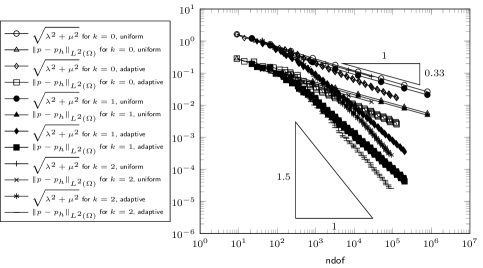
Figure 2: Errors and error estimators from Subsection 8.1.

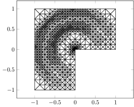
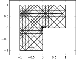
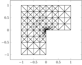
Figure 3: Adaptively refined triangulations for the experiment from Subsection 8.1.

8.2 L-shaped domain, II

For $f\equiv-1$ and $u_{D}\equiv 0$ define $\varphi(x,y):=(1/2)(x,y)$ with $-\operatorname{div}\varphi=f$.

The error estimators are plotted against the degrees of freedom in Figure 4 for $k=0,1,2$. The error estimators show for $k=0,1,2$ a suboptimal convergence rate of $h^{2/3}\approx\texttt{ndof}^{-1/3}$ for uniform refinement. The adaptive algorithm 6.1 recovers the optimal convergence rate of $\texttt{ndof}^{-(k+1)/2}$. Adaptively refined meshes are depicted in Figure 5 for approximately 1000 degrees of freedom. The strong refinement towards the singularity at the re-entrant corner is clearly visible. The smoothness of $\varphi\in P_{1}(\Omega;\mathbb{R}^{2})$ implies that the data-approximation error estimator $\mu_{\ell}$ vanishes on all triangulations for $k=1,2$. For $k=0$, $\mu_{\ell}$ does not vanish, nevertheless, since $\mu_{\ell}^{2}\leq\kappa\lambda_{\ell}^{2}$ for all $\ell$, only the Dörfler marking is applied.

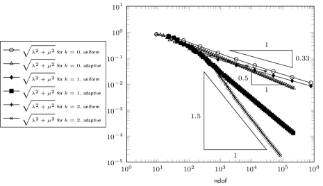
Figure 4: Error estimators for the experiment from Subsection 8.2.

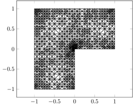
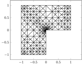
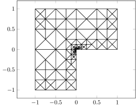
Figure 5: Adaptively refined triangulations for the experiment from Subsection 8.2.

8.3 Singular $\alpha$

This subsection is devoted to a numerical investigation of the dependence of the error $\|p-p_{h}\|_{L^{2}(\Omega)}$ on the regularity of $\alpha$. The exact smooth solution $u\in C^{\infty}(\Omega)$ of

$$-\Delta u=2\sin(\pi x)\sin(\pi y)\text{ in }\Omega\qquad\text{and}\qquad u|_{\Gamma_{D}}=0$$

reads $u(x,y)=\sin(\pi x)\sin(\pi y)$. Define $\varphi=\nabla u+\operatorname{Curl}(\widetilde{\alpha})$ with $\widetilde{\alpha}\in H^{1}(\Omega)\setminus H^{2}(\Omega)$ defined by $\widetilde{\alpha}(r,\phi)=r^{2/3}\sin(2\phi/3)$. Then $\varphi\in H(\operatorname{div},\Omega)$ with $-\operatorname{div}\varphi=f$.

The errors and error estimators are plotted in Figure 6 against the number of degrees of freedom. The convergence rate on uniform red-refined meshes for $k=1,2$ is $h^{2/3}\approx\texttt{ndof}^{-1/3}$ and, hence, the convergence rate seems to depend on the regularity of $\alpha$. The errors and error estimators show the same convergence rate. Figure 7 focuses on the results for $k=0$ and uniform mesh-refinement. The error $\|p-p_{h}\|_{L^{2}(\Omega)}$ and the error estimator $\sqrt{\lambda^{2}+\mu^{2}}$ show a convergence rate between $h$ and $h^{2/3}$, while $\left\|\operatorname{Curl}(\alpha-\alpha_{h})\right\|_{L^{2}(\Omega)}$ converges with a rate of $h^{2/3}\approx\texttt{ndof}^{-1/3}$ due to the singularity of $\alpha$. This numerical experiment suggests that the error $\|p-p_{h}\|_{L^{2}(\Omega)}$ does not depend on the regularity of $\alpha$ (at least in a preasymptotic regime). The triangle inequality implies $\left\|\operatorname{Curl}(\alpha-\alpha_{h})\right\|_{L^{2}(\Omega)}\leq\|p-p_{h}\|_{L^{2}(\Omega)}+\mu$. This upper bound is also plotted in Figure 7.

Figure 8 depicts adaptively refined meshes for $k=0,1,2$ with approximately 1000 degrees of freedom. The singularity of $\alpha$ leads to a strong refinement towards the re-entrant corner. The marking with respect to the data-approximation ($\mu_{\ell}^{2}>\kappa\lambda_{\ell}^{2}$ in Algorithm 6.1) is only applied at levels 1–5, 7, 12, and 18 for $k=0$. All other marking steps for $k=0,1,2$ use the Dörfler marking ($\mu_{\ell}^{2}\leq\kappa\lambda_{\ell}^{2}$).

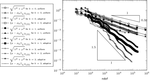
Figure 6: Errors and error estimators for the experiment with singular $\alpha$ from Subsection 8.3.

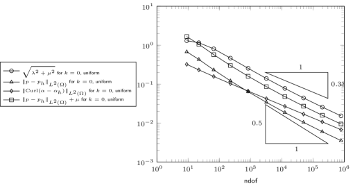
Figure 7: Errors and error estimators for the experiment with singular $\alpha$ from Subsection 8.3 and uniform refinement.

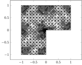
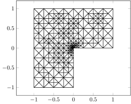
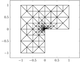
Figure 8: Adaptively refined triangulations for the experiment from Subsection 8.3.

References

- [1] A. Alonso Rodríguez, R. Hiptmair, and A. Valli. Mixed finite element approximation of eddy current problems. IMA J. Numer. Anal., 24(2):255–271, 2004.
- [2] C. Amrouche, C. Bernardi, M. Dauge, and V. Girault. Vector potentials in three-dimensional non-smooth domains. Math. Methods Appl. Sci., 21(9):823–864, 1998.
- [3] D. N. Arnold and F. Brezzi. Mixed and nonconforming finite element methods: implementation, postprocessing and error estimates. RAIRO Modél. Math. Anal. Numér., 19(1):7–32, 1985.
- [4] D. N. Arnold and R. S. Falk. A uniformly accurate finite element method for the Reissner-Mindlin plate. SIAM J. Numer. Anal., 26(6):1276–1290, 1989.
- [5] D. N. Arnold, R. S. Falk, and R. Winther. Preconditioning in and applications. Math. Comp., 66(219):957–984, 1997.
- [6] R. Becker, S. Mao, and Z. Shi. A convergent nonconforming adaptive finite element method with quasi-optimal complexity. SIAM J. Numer. Anal., 47(6):4639–4659, 2010.
- [7] P. Binev, W. Dahmen, and R. DeVore. Adaptive finite element methods with convergence rates. Numer. Math., 97(2):219–268, 2004.
- [8] P. Binev and R. DeVore. Fast computation in adaptive tree approximation. Numer. Math., 97(2):193–217, 2004.
- [9] D. Boffi, F. Brezzi, and M. Fortin. Mixed Finite Element Methods and Applications, volume 44 of Springer Series in Computational Mathematics. Springer, Heidelberg, 2013.
- [10] S. C. Brenner and L. R. Scott. The Mathematical Theory of Finite Element Methods, volume 15 of Texts in Applied Mathematics. Springer Verlag, New York, Berlin, Heidelberg, 3 edition, 2008.
- [11] F. Brezzi. On the existence, uniqueness and approximation of saddle-point problems arising from Lagrangian multipliers. Rev. Française Automat. Informat. Recherche Opérationnelle Sér. Rouge, 8(R-2):129–151, 1974.
- [12] F. Brezzi, M. Fortin, and R. Stenberg. Error analysis of mixed-interpolated elements for Reissner-Mindlin plates. Math. Models Methods Appl. Sci., 1(2):125–151, 1991.
- [13] C. Carstensen, M. Feischl, M. Page, and D. Praetorius. Axioms of adaptivity. Comput. Math. Appl., 67(6):1195–1253, 2014.
- [14] C. Carstensen, D. Gallistl, and M. Schedensack. Adaptive nonconforming Crouzeix-Raviart FEM for eigenvalue problems. Math. Comp., 84(293):1061–1087, 2015.
- [15] C. Carstensen, D. Peterseim, and M. Schedensack. Comparison results of finite element methods for the Poisson model problem. SIAM J. Numer. Anal., 50(6):2803–2823, 2012.
- [16] C. Carstensen and H. Rabus. Axioms of adaptivity for separate marking. 2015. In preparation, private communication.
- [17] C. Carstensen and M. Schedensack. Medius analysis and comparison results for first-order finite element methods in linear elasticity. IMA J. Numer. Anal., 2014. Published online.
- [18] J. M. Cascon, C. Kreuzer, R. H. Nochetto, and K. G. Siebert. Quasi-optimal convergence rate for an adaptive finite element method. SIAM J. Numer. Anal., 46(5):2524–2550, 2008.
- [19] P. G. Ciarlet. The Finite Element Method for Elliptic Problems. Studies in Mathematics and its Applications, Vol. 4. North-Holland Publishing Co., Amsterdam-New York-Oxford, 1978.
- [20] M. Crouzeix and R. S. Falk. Nonconforming finite elements for the Stokes problem. Math. Comp., 52(186):437–456, 1989.
- [21] M. Crouzeix and P.-A. Raviart. Conforming and nonconforming finite element methods for solving the stationary Stokes equations. I. Rev. Française Automat. Informat. Recherche Opérationnelle Sér. Rouge, 7(R-3):33–75, 1973.
- [22] M. Fortin. A three-dimensional quadratic nonconforming element. Numer. Math., 46(2):269–279, 1985.
- [23] M. Fortin and M. Soulie. A nonconforming piecewise quadratic finite element on triangles. Internat. J. Numer. Methods Engrg., 19(4):505–520, 1983.
- [24] V. Girault and P.-A. Raviart. Finite Element Methods for Navier-Stokes Equations, volume 5 of Springer Series in Computational Mathematics. Springer-Verlag, Berlin, 1986.
- [25] T. Gudi. A new error analysis for discontinuous finite element methods for linear elliptic problems. Math. Comp., 79(272):2169–2189, 2010.
- [26] J. Huang and Y. Xu. Convergence and complexity of arbitrary order adaptive mixed element methods for the Poisson equation. Sci. China Math., 55(5):1083–1098, 2012.
- [27] L. D. Marini. An inexpensive method for the evaluation of the solution of the lowest order Raviart-Thomas mixed method. SIAM J. Numer. Anal., 22(3):493–496, 1985.
- [28] G. Matthies and L. Tobiska. Inf-sup stable non-conforming finite elements of arbitrary order on triangles. Numer. Math., 102(2):293–309, 2005.
- [29] J. M. L. Maubach and P. J. Rabier. Nonconforming finite elements of arbitrary degree over triangles. RANA : Reports on applied and numerical analysis, Technische Universiteit Eindhoven, 2003.
- [30] J.-C. Nédélec. Mixed finite elements in . Numer. Math., 35(3):315–341, 1980.
- [31] J.-C. Nédélec. A new family of mixed finite elements in . Numer. Math., 50(1):57–81, 1986.
- [32] H. Rabus. A natural adaptive nonconforming FEM of quasi-optimal complexity. Comput. Methods Appl. Math., 10(3):315–325, 2010.
- [33] R. Rannacher and S. Turek. Simple nonconforming quadrilateral Stokes element. Numer. Methods Partial Differential Equations, 8(2):97–111, 1992.
- [34] P.-A. Raviart and J. M. Thomas. A mixed finite element method for 2nd order elliptic problems. In Mathematical Aspects of Finite Element Methods (Proc. Conf., Consiglio Naz. delle Ricerche (C.N.R.), Rome, 1975), pages 292–315. Springer, Berlin, 1977.
- [35] W. Rudin. Principles of Mathematical Analysis. McGraw-Hill Book Co., New York-Auckland-Düsseldorf, third edition, 1976.
- [36] M. Schedensack. A new discretization for th-Laplace equations with arbitrary polynomial degrees. 2015. Preprint, arXiv:1512.06513.
- [37] M. Schedensack. Mixed finite element methods for linear elasticity and the Stokes equations based on the Helmholtz decomposition. 2016. In preparation.
- [38] J. Schöberl. A posteriori error estimates for Maxwell equations. Math. Comp., 77(262):633–649, 2008.
- [39] L. R. Scott and S. Zhang. Finite element interpolation of nonsmooth functions satisfying boundary conditions. Math. Comp., 54(190):483–493, 1990.
- [40] R. Stevenson. The completion of locally refined simplicial partitions created by bisection. Math. Comp., 77(261):227–241, 2008.
- [41] G. Stoyan and Á. Baran. Crouzeix-Velte decompositions for higher-order finite elements. Comput. Math. Appl., 51(6-7):967–986, 2006.
- [42] A. Veeser. Approximating gradients with continuous piecewise polynomial functions. Foundations of Computational Mathematics, pages 1–28, 2014.
- [43] R. Verfürth. A Review of a Posteriori Error Estimation and Adaptive Mesh-Refinement Techniques. Advances in numerical mathematics. Wiley, 1996.
- [44] L. Zhong, L. Chen, S. Shu, G. Wittum, and J. Xu. Convergence and optimality of adaptive edge finite element methods for time-harmonic Maxwell equations. Math. Comp., 81(278):623–642, 2012.