Optimization of nonlocal time-delayed feedback controllers

Abstract

A class of Pyragas type nonlocal feedback controllers with time-delay is investigated for the Schlögl model. The main goal is to find an optimal kernel in the controller such that the associated solution of the controlled equation is as close as possible to a desired spatio-temporal pattern. An optimal kernel is the solution to a nonlinear optimal control problem with the kernel taken as control function. The well-posedness of the optimal control problem and necessary optimality conditions are discussed for different types of kernels. Special emphasis is laid on time-periodic functions as desired patterns. Here, the cross correlation between the state and the desired pattern is invoked to set up an associated objective functional that is to be minimized. Numerical examples are presented for the 1D Schlögl model and a class of simple step functions for the kernel.

1 Introduction

In this paper, we consider a class of nonlocal feedback controllers with application to the control of certain nonlinear partial differential equations. The research on feedback control laws of this type has become quite active in theoretical physics for stabilizing wave-type solutions of reaction-diffusion systems such as the Schlögl model (also known as Nagumo or Chafee-Infante equation) or the FitzHugh-Nagumo system.

The controllers can be characterized as follows: First of all, they are a generalization of Pyragas type controllers that became very popular in the past. We refer to pyragas1992 , pyragas2006 , and the survey volume schoell_schuster2008 . In the simplest form of Pyragas type feedback control, the difference of the current state $u(x,t)$ and the retarded state $u(x,t-\tau)$, multiplied with a real number $\kappa$, is taken as control, i.e. the feedback control $f$ is

$$f(x,t):=\kappa\,(u(x,t)-u(x,t-\tau)),$$

where $\tau$ is a fixed time delay and $\kappa$ is the feedback gain.

In the nonlocal generalization we consider in this paper, the feedback control is set up by an integral operator of the form

$$f(x,t):=\kappa\,\left(\int_{0}^{T}g(\tau)u(x,t-\tau)\,d\tau-u(x,t)\right).$$ (1)

Here, different time delays appear in a distributed way. Depending on the particular choice of the kernel $g$, various spatio-temporal patterns of the controlled solution $u$ can be achieved. We refer to bachmair_schoell14 ; loeber_etal2014 ; siebert_schoell14 , and siebert_alonso_baer_schoell14 with application to the Schlögl model and to atay2003 ; kyrichenko_blyuss_schoell2014 ; wille_lehnert_schoell2014 with respect to control of ordinary differential equations.

Our main goal is the selection of the kernel $g$ in an optimal way. We want to achieve a desired spatio-temporal pattern for the resulting state function and look for an optimal feedback kernel $g$ to approximate this pattern as closely as possible. For this purpose, in the second half of the paper we will concentrate on a particular choice of $g$ as a step function.

We are optimizing feedback controllers but we shall apply methods of optimal control to achieve our goal. This leads to new optimal control problems for reaction-diffusion equations containing nonlocal terms with time delay in the state equation. We develop the associated necessary optimality conditions and discuss numerical approaches for solving the problems posed. Working on this class of problems, we observed that standard quadratic tracking type objective functionals are possibly not the right tool for approximating desired time-periodic patterns. We found out that the so-called cross correlation partially better fits to our goals. We report on our numerical tests at the end of this paper.

This research contributes results to the optimal control of nonlinear reaction diffusion equations, where wave type solutions such as traveling wave fronts or spiral waves occur in unbounded domains. We mention the papers borzi_griesse06 ; brandao_etal08 ; ckp09 on the optimal control of systems that develop spiral waves or kun_nag_cha_wag2011 ; kunisch_wagner2012-3 ; kunisch_wang12 on systems with heart medicine as background. Moreover, we refer to buch_eng_kamm_tro2013 ; casas_ryll_troeltzsch2014b , where different numerical and theoretical aspects of optimal control of the Schlögl or FitzHugh-Nagumo equations are discussed. It is a characteristic feature of such systems that the computed optimal solutions might be unstable with respect to perturbations in the data, in particular initial data.

Feedback control aims at generating stable solutions. Various techniques of feedback control are known, we refer only to the monographies coron07 ; lasiecka_triggiani2000a ; lasiecka_triggiani2000b ; Krstic2010 and to the references cited therein. Moreover, we mention gugat_troeltzsch2013 on feedback stabilization for the Schlögl model. Pyragas type feedback control is one associated field of research that became very active, cf. schoell_schuster2008 for an account on current research in this field. In associated publications, the feedback control laws were considered as given. For instance, the kernel in nonlocal delayed feedback was given and it was studied what kind of patterns arise from different choices of the kernel.

The novelty of our paper is that we study an associated inverse (say design) problem: Find a kernel such that the associated feedback solution best approximates a desired pattern.

2 Two models of feedback control

We consider the following semilinear parabolic equation with reaction term $R$ and control function (forcing) $f$,

$$\partial_{t}u-\Delta u+R(u)=f$$ (1)

subject to appropriate initial and boundary conditions in a spatio-temporal domain $\Omega\times(0,T)$. Using a feedback control in the form (1), we arrive at the following nonlinear initial-boundary value problem that includes a nonlocal term with time delay,

$$\begin{array}[]{rcll}\partial_{t}u(x,t)-\Delta u(x,t)+R(u(x,t))&=&\displaystyle\kappa\left(\int_{0}^{T}g(\tau)u(x,t-\tau)\,d\tau-u(x,t)\right)&\mbox{in }\Omega,\\[8.61108pt] u(x,s)&=&u_{0}(x,s)&\mbox{in }\Omega,\\[4.30554pt] \displaystyle{\partial_{n}u}(x,t)&=&0&\mbox{on }\Gamma,\end{array}$$ (2)

for almost all $t\in(0,T),\,s\in[-T,0]$.

Here, $\partial_{n}$ denotes the outward normal derivative on $\Gamma=\partial\Omega$. We want to determine a feedback kernel $g\in L^{\infty}(0,T)$ such that the solution $u$ to (2) is as close as possible to a desired function $u_{d}$. The function $g$ will have to obey certain restrictions, namely

$$0\leq g(t) \leq \beta\quad\mbox{ a.e. on }[0,T],$$ (3)

$$\displaystyle\int_{0}^{T}g(s)\,ds = 1,$$ (4)

where $\beta>0$ is a given (large) positive constant. This upper bound is chosen to have a uniform bound for $g$. It is needed for proving the solvability of the optimal control problem.

We shall present the main part of our theory for the general type of $g$ defined above. In our numerical computations, however, we will concentrate on functions $g$ of the following particular form: We select $t_{1},\,t_{2}$ such that $0\leq t_{1}<t_{2}\leq T$, $t_{2}-t_{1}\geq\delta>0$ and define

$$g(t)=\left\{\begin{array}[]{cl}\displaystyle\frac{1}{t_{2}-t_{1}},&t_{1}\leq t\leq t_{2}\\[8.61108pt] 0,&\mbox{elsewhere}.\end{array}\right.$$ (5)

It is obvious that $g$ satisfies the constraints (3),(4) with $\beta=1/\delta$. Using this form for $g$, we end up with the particular feedback equation

$$\partial_{t}u(x,t)-\Delta u(x,t)+R(u(x,t))=\kappa\,\left(\frac{1}{t_{2}-t_{1}}\int_{t_{1}}^{t_{2}}u(x,t-\tau)\,d\tau-u(x,t)\right).$$ (6)

In (6), we will also vary $\kappa$ in the state equation as part of the control variables to be optimized. In contrast to this, $\kappa$ is assumed to be fixed in the model with a general control function $g$. In the special model, we have a restricted flexibility in the optimization, because only the real numbers $k,\,t_{1},\,t_{2}$ can be varied. Yet, we are able to generate a class of interesting time-periodic patterns.

Throughout the paper we will rely on the following

Assumptions. The set $\Omega\subset\mathbb{R}^{N}$, $N\leq 3$, is a bounded Lipschitz domain; for $N=1$, we set $\Omega=(a,b)$. By $T>0$, a finite terminal time is fixed. In theoretical physics, also the choice $T=\infty$ is of interest. However, we do not investigate the associated analysis, because an infinite time interval requires the use of more complicated function spaces. Moreover, the restriction to a bounded interval fits better to the numerical computations. Throughout the paper, we use the notation $Q:=\Omega\times(0,T)$ and $\Sigma=\Gamma\times(0,T)$. for the space-time cylinder.

Remark 1

We will often use the term ”wave type solution” or ”traveling wave”. This is a function $(x,t)\mapsto u(x,t)$ that can be represented in the form $u(x,t)=v(x-c\,t)$ with some other smooth function $v$. Here, $c$ is the velocity of the wave type solution. Such solutions are known to exist in $\Omega=\mathbb{R}$ but not in in a bounded interval $\Omega=(a,b)$.

In our paper, the terms ” wave type solution” or ”traveling wave” stand for solutions of the Schlögl model in the bounded domain $(a,b)$. We use these terms, since the computed solutions exhibit a similar behavior as associated solutions in $\Omega=\mathbb{R}$.

The reaction term $R$ is defined by

$$R(u)=\rho\,(u-u_{1})(u-u_{2})(u-u_{3}),$$ (7)

where $u_{1}\leq u_{2}\leq u_{3}$ and $\rho>0$ are fixed real numbers. In our computational examples, we will take $\rho:=1$. The numbers $u_{i}$, $i=1,\ldots,3$, define the fixed points of the (uncontrolled) Schlögl model (1). In view of the time delay, we have to provide initial values $u_{0}$ for $u$ in the interval $[-T,0]$ for the general model (2) and in $[-t_{2},0]$ for the special model (6). We assume $u_{0}\in C(\bar{\Omega}\times[-T,0])$ or $u_{0}\in C(\bar{\Omega}\times[-t_{2},0])$, respectively. The desired state $u_{d}$ is assumed to be bounded and measurable on $Q$.

3 Well-posedness of the feedback equation

In this section, we prove the existence and uniqueness of a solution to the general feedback equation (2). To this aim, we first reduce the equation to an inhomogeneous initial-boundary value problem. For $t\in[0,T]$, we write

$$\int_{0}^{T}g(\tau)u(x,t-\tau)\,d\tau = \int_{0}^{t}g(\tau)u(x,t-\tau)\,d\tau+\underbrace{\int_{t}^{T}g(\tau)u(x,t-\tau)\,d\tau}_{=:U_{g}(x,t)}$$

$$= \int_{0}^{t}g(\tau)u(x,t-\tau)\,d\tau+U_{g}(x,t).$$

The function $U_{g}$ is associated with the fixed initial function $u_{0}$ and is defined by

$$U_{g}(x,t)=\int_{t}^{T}g(\tau)u_{0}(x,t-\tau)\,d\tau;$$

notice that we have $t-\tau\leq 0$ in the integral above. By the assumed continuity of $u_{0}$, the function $U_{g}$ belongs to $C(\bar{\Omega}\times[0,T])$.

Next, for given $g\in L^{2}(0,T)$, we introduce a linear integral operator $K(g):L^{2}(Q)\to L^{2}(Q)$ by

$$(K(g)u)(x,t):=\int_{0}^{t}g(\tau)u(x,t-\tau)\,d\tau.$$ (8)

Substituting $s=t-\tau$, we obtain the equivalent representation

$$(K(g)u)(x,t)=\int_{0}^{t}g(t-s)u(x,s)\,ds.$$

Inserting $U_{g}$ and $K(g)$ in the state equation (2), we obtain the following nonlocal initial-boundary value problem:

$$\left\{\begin{array}[]{rcll}\partial_{t}u-\Delta u+R(u)+\kappa\,u-\kappa\,K(g)u&=&\kappa\,U_{g}&\mbox{in }Q,\\[4.30554pt] u(x,0)&=&u_{0}(x,0)&\mbox{in }\Omega,\\[4.30554pt] \partial_{n}u&=&0&\mbox{on }\Sigma.\end{array}\right.$$ (9)

In the next theorem, we use the Sobolev space

$$W(0,T)=L^{2}(0,T;H^{1}(\Omega))\cap H^{1}(0,T;L^{2}(\Omega)).$$

Theorem 3.1

For all $g\in L^{\infty}(0,T)$, $U_{g}\in L^{p}(Q),\,p>\frac{5}{2},$ and $u_{0}\in C(\bar{\Omega}\times[-T,0])$, the problem (9) has a unique solution $u\in W(0,T)\cap C(\bar{Q})$.

Proof

We use the same technique that was applied in casas_ryll_troeltzsch2014 to show the existence and continuity of the solution to the FitzHugh-Nagumo system. Let us mention the main steps. First, we apply a simple transformation that is well-known in the theory of evolution equations. We set

$$u=e^{\lambda t}v$$

with some $\lambda>0$. This transforms the partial differential equation in (9) to an equation for the new unknown function $v$,

$$v_{t}-\Delta v+e^{-\lambda t}R(e^{\lambda t}v)+(\lambda+\kappa)v=\kappa\,K_{\lambda}(g)v+e^{-\lambda t}\kappa\,U_{g},$$ (10)

where the integral operator $K_{\lambda}(g)$ is defined by

$$(K_{\lambda}(g)v)(x,t)=\int_{0}^{t}e^{-\lambda(t-s)}g(t-s)v(x,s)\,ds.$$

If $g\in L^{\infty}(0,T)$, then both operators $K(g)$ and $K_{\lambda}(g)$ are continuous linear operators in $L^{p}(Q)$, for all $p\geq 1$. Moreover, due to the factor $e^{-\lambda(t-s)}$, the norm of $K_{\lambda}(g):L^{2}(Q)\to L^{2}(Q)$ tends to zero as $\lambda\to\infty$. We obtain

$$\|K_{\lambda}(g)\|_{\mathcal{L}(L^{2}(Q))}\leq\frac{c}{\sqrt{\lambda}}\|g\|_{L^{\infty}(0,T)}$$ (11)

with some constant $c>0$. To have this estimate, we assumed in (3) that $g$ is uniformly bounded by the constant $\beta$. If $\lambda$ is sufficiently large, then we have

$$\int_{Q}[e^{-\lambda t}R(e^{\lambda t}v)+(\lambda+\kappa)v-\kappa K_{\lambda}(g)v]\,v\,dxdt\geq\frac{\lambda}{2}\|v\|^{2}_{L^{2}(Q)}\quad\forall v\in L^{2}(Q),$$

because the coercive term $(\lambda+\kappa)\,v$ in the left side is dominating the other terms, cf. casas_ryll_troeltzsch2014 .

With this inequality, an a priori estimate can be derived in $L^{2}(Q)$ for any solution $v$ of the equation (9). Now, we can proceed as in casas_ryll_troeltzsch2014 : A fixed-point principle is applied in $L^{2}(Q)$ to prove the existence and uniqueness of the solution $v$ that in turn implies the same for $u$. For the details, the reader is referred to casas_ryll_troeltzsch2014 , proof of Theorem 2.1. However, we mention one important idea: Thanks to (11), the term $(\lambda+\kappa)$ absorbes the non-monotone terms in the equation (10) so that, in estimations, equation (10) behaves like the parabolic equation

$$v_{t}-\Delta v+\tilde{R}(v)=F$$

with a monotone non-decreasing nonlinearity $\tilde{R}$ and given right-hand side $F\in L^{p}(Q)$, $p>5/2$. This fact can be exploited to verify, for each $r>0$, the existence of a constant $C_{r}>0$ with the following property: If $g\in L^{\infty}(Q)$ obeys $\|g\|_{L^{\infty}(Q)}\leq r$ and $u$ is the associated solution to (2), then

$$\|u\|_{L^{\infty}(Q)}\leq C_{r}.$$ (12)

$\Box$

4 Analysis of optimization problems for feedback controllers

4.1 Definition of two optimization problems

General kernel as control

Let a desired function $u_{d}\in L^{\infty}(Q)$ be given. In our later applications, $u_{d}$ models a desired spatio-temporal pattern. Moreover, we fix a non-negative function $c_{Q}\in L^{\infty}(Q)$. This function is used for selecting a desired observation domain. We consider the feedback equation (2) and want to find a kernel $g$ such that the associated solution $u$ approximates $u_{d}$ as close as possible in the domain of observation. This goal is expressed by the following functional $j:L^{2}(Q)\times L^{\infty}(0,T)\to\mathbb{R}$ that is to be minimized,

$$j(u,g):=\frac{1}{2}\iint_{Q}c_{Q}(u-u_{d})^{2}\,dxdt+\frac{\nu}{2}\int_{0}^{T}g^{2}(t)\,dt.$$

Here, $\nu\geq 0$ is a Tikhonov regularization parameter. The standard choice of $c_{Q}$ is $c_{Q}(x,t)=1$ for all $(x,t)\in Q$. Another selection will be applied for periodic functions $u_{d}$: $c(x,t)=1$ for all $(x,t)\in Q$ with $t\geq T/2$ and $c(x,t)=0$ for all $(x,t)\in Q$ with $t<T/2$.

By Theorem 3.1, to each $g\in L^{\infty}(0,T)$ there exists a unique associated state function $u$ that will be denoted by $u_{g}$. Then $j$ does only depend on $g$ and we obtain the reduced objective functional $J$,

$$J:g\mapsto j(u_{g},g).$$

Therefore, our general optimization problem can be formulated as follows:

$$\min_{g\in C}J(g):=\frac{1}{2}\iint_{Q}c_{Q}(u_{g}-u_{d})^{2}\,dxdt+\frac{\nu}{2}\int_{0}^{T}g^{2}(t)\,dt,$$

where $C\subset L^{\infty}(0,T)$ is the convex and closed set defined by

$$C:=\left\{g\in L^{\infty}(0,T):\ 0\leq g(t)\leq\beta\;\mbox{ a.e. in }[0,T]\mbox{ and }\int_{0}^{T}g(t)\,dt=1.\right\}$$

Notice that $C$ is a weakly compact subset of $L^{2}(0,T)$. The restrictions on $g$ are motivated by the background in mathematical physics. In particular, the restriction on the integral of $g$ guarantees that

$$\int_{0}^{T}g(\tau)u(x,t-\tau)\,d\tau-u(x,t)=0,$$

if $u(x,t-\tau)=u(x,t)$ in Q. By the definition of $u_{g}$, the optimization is subject to the state equation (2).

Special kernel as control

The other optimization problem we are interested in, uses the particular form (5) of the kernel $g$,

$$\min_{0\leq t_{1}<t_{2}\leq T}J_{S}(\kappa,t_{1},t_{2}):=\frac{1}{2}\iint_{Q}c_{Q}(u_{(\kappa,t_{1},t_{2})}-u_{d})^{2}\,dxdt+\frac{\nu}{2}(t_{1}^{2}+t_{2}^{2}+\kappa^{2}),$$

where $u_{(\kappa,t_{1},t_{2})}$ is the solution of (6) for a given triplet $(\kappa,t_{1},t_{2})$. This problem might fail to have an optimal solution, because the set of admissible triplets $(\kappa,t_{1},t_{2})$ is not closed. Notice that we need $t_{1}<t_{2}$ in (6). Therefore, we fix $\delta>0$ and define the slightly changed admissible set

$$C_{\delta}:=\left\{(\kappa,t_{1},t_{2})\in\mathbb{R}^{3}:\ 0\leq t_{1}<t_{2}\leq T,\,t_{2}-t_{1}\geq\delta,\ \kappa\in\mathbb{R}\right\}$$

that is compact. In this way, we obtain the special finite-dimensional optimization problem for step functions $g$,

$$\min_{(\kappa,t_{1},t_{2})\in C_{\delta}}J_{S}(\kappa,t_{1},t_{2}):=\frac{1}{2}\iint_{Q}c_{Q}(u_{(\kappa,t_{1},t_{2})}-u_{d})^{2}\,dxdt+\frac{\nu}{2}(t_{1}^{2}+t_{2}^{2}+\kappa^{2}).$$

4.2 Discussion of (PG)

The control-to-state mapping $G$

Next, we discuss the differentiability of the control-to-state mappings $g\mapsto u_{g}$ and $(\kappa,t_{1},t_{2})\mapsto u(\kappa,t_{1},t_{2})$. First, we consider the case of the general kernel $g$. The analysis for the particular kernel (5) is fairly analogous but cannot deduced as a particular case of (PG). We will briefly sketch it in a separate section.

By Theorem 3.1, we know that the mapping $G:g\mapsto u_{g}$ is well defined from $L^{\infty}(0,T)$ to $C(\bar{Q})$. Now we discuss the differentiability of $G$. To slightly simplify the notation, we introduce an operator $\mathcal{K}:L^{\infty}(0,T)\times C(\bar{Q})\to C(\bar{Q})$ by

$$\mathcal{K}(g,u)=K(g)u,$$

where $K(g)$ was introduced in (8); notice that $\mathcal{K}$ is bilinear. Let us first show the differentiability for $\mathcal{K}$.

We fix $g\in L^{\infty}(0,T),\,u\in C(\bar{Q})$, and select varying increments $h\in L^{\infty}(0,T)$, $v\in C(\bar{Q})$. Then we have

$$\begin{split}&\mathcal{K}(g+h,u+v)=\int_{0}^{T}[g(\tau)+h(\tau)][u(x,t-\tau)+v(x,t-\tau)]\,d\tau\\ &\quad=\int_{0}^{t}g(\tau)u(x,t-\tau)\,d\tau+\underbrace{\int_{0}^{t}h(\tau)u(x,t-\tau)\,d\tau+\int_{0}^{t}g(\tau)v(x,t-\tau)\,d\tau}_{A(g,u)(h,v)}\\ &\quad\qquad+\underbrace{\int_{0}^{t}h(\tau)v(x,t-\tau)\,d\tau}_{R(h,v)}={\mathcal{K}(g,u)}+A(g,u)(h,v)+{R(h,v)},\end{split}$$

where $A(g,u):L^{\infty}(0,T)\times C(\bar{Q})\to C(\bar{Q})$ is a linear continuous operator and $R:L^{\infty}(0,T)\times C(\bar{Q})\to C(\bar{Q})$ is a remainder term. It is easy to confirm that

$$\frac{\|R(h,v)\|_{C(\bar{Q})}}{\|(h,v)\|_{L^{\infty}(0,T)\times C(\bar{Q})}}\to 0,\quad\mbox{ if }\|(h,v)\|_{L^{\infty}(0,T)\times C(\bar{Q})}\to 0.$$

Therefore, $\mathcal{K}$ is Fréchet-differentiable. As a continuous bilinear form, $\mathcal{K}$ is also of class $C^{2}$.

Now, we investigate the control-to-state mapping $G:L^{\infty}(0,T)\to C(\bar{Q})$ defined by $G:g\mapsto u_{g},$ where the state function $u_{g}$ is defined as the unique solution to

$$\begin{array}[]{rcll}\partial_{t}u-\Delta u+R(u)+\kappa\,u&=&\kappa\,\mathcal{K}(g,u)+\kappa\,U_{g}&\text{ in }Q\\ \partial_{n}u&=&0&\text{ in }\Sigma\\ u(0)&=&u_{0}(0)&\text{ in }\Omega.\end{array}$$ (12)

In what follows, the initial function $u_{0}$ will be kept fixed and is therefore not mentioned. Of course, $U_{g},\,G$ and some of the operators below depend on $u_{0}$, but we will not explicitely mention this dependence. To discuss $G$, we need known properties of the following auxiliary mapping $\mathcal{G}:v\mapsto u$, where

$$\begin{array}[]{rcll}\partial_{t}u-\Delta u+R(u)+\kappa\,u&=&v&\text{ in }Q\\ \partial_{n}u&=&0&\text{ in }\Sigma\\ u(0)&=&u_{0}(0)&\text{ in }\Omega.\end{array}$$

This mapping $\mathcal{G}$ is of class $\mathcal{C}^{2}$ from $L^{p}(Q)$ to $W(0,T)\cap\mathcal{C}(\bar{Q})$, if $p>\frac{5}{2}$, in particular from $L^{\infty}(Q)$ to $L^{\infty}(Q)$, cf. casas_ryll_troeltzsch2014 or, for monotone $R$, cas93 , rayzid99 , tro10book .

Now (consider $v:=\kappa\,(\mathcal{K}(g,u)+U_{g})$ as given and keep the initial function $u_{0}$ fixed), $u$ solves (12) if and only if $u=\mathcal{G}(\kappa\,\mathcal{K}(g,u)+\kappa\,U_{g})$, i.e.

$$u-\mathcal{G}(\kappa\,\mathcal{K}(g,u)+\kappa\,U_{g})=0.$$ (13)

We introduce a new mapping $\mathcal{F}\,:\,L^{\infty}(Q)\times L^{\infty}(0,T)\to L^{\infty}(Q)$ defined by

$$\mathcal{F}(u,g):=u-\mathcal{G}(\kappa\,\mathcal{K}(g,u)+\kappa\,U_{g}).$$

Then, (13) is equivalent to the equation

$$\mathcal{F}(u,g)=0.$$ (14)

We have proved above that the mapping $(g,u)\mapsto\mathcal{K}(g,u)$ is of class $\mathcal{C}^{2}$ from $L^{\infty}(0,T)\times L^{\infty}(Q)$ to $L^{\infty}(Q)$. Obviously, also the linear mapping $g\mapsto U_{g}$ is of class $\mathcal{C}^{2}$ from $L^{\infty}(0,T)$ to $L^{\infty}(Q)$. By the chain rule, also $\mathcal{F}$ is $\mathcal{C}^{2}$ from $L^{\infty}(Q)\times L^{\infty}(0,T)\to L^{\infty}(Q)$ and the mappings $\partial_{g}\mathcal{F}(\bar{u},\bar{g})$, $\partial_{u}\mathcal{F}(\bar{u},\bar{g})$ are continuous in the associated pairs of spaces.

To use the implicit function theorem, we prove that $\partial_{u}\mathcal{F}(\bar{u},\bar{g})$ is continuously invertible at any fixed pair $(\bar{u},\bar{g})$. Therefore, we consider the equation

$$\partial_{u}\mathcal{F}(\bar{u},\bar{g})v=z$$ (15)

with given right-hand side $z\in L^{\infty}(Q)$ and show the existence of a unique solution $v\in L^{\infty}(Q)$. The equation is equivalent with

$$v-\mathcal{G}^{\prime}(\underbrace{\kappa\,\mathcal{K}(\bar{g},\bar{u})+\kappa\,U_{g}}_{\bar{p}})\kappa\,\mathcal{K}(g,v)=z.$$ (16)

Writing for convenience $\bar{p}=\kappa\,\mathcal{K}(\bar{g},\bar{u})+\kappa\,U_{g}$, we obtain the simpler form

$$v-\mathcal{G}^{\prime}(\bar{p})\kappa\,K(\bar{g})v=z.$$

A function $z\in L^{\infty}(Q)$ does not in general belong to $W(0,T)$. To overcome this difficulty, we set $w:=v-z$ and transform the equation to

$$w=\mathcal{G}^{\prime}(\bar{p})\underbrace{\kappa\,K(\bar{g})(w+z)}_{q}=\mathcal{G}^{\prime}(\bar{p})q.$$ (17)

where $q:=\kappa\,K(\bar{g})(w+z)$. As the next result shows, $w$ is the solution of a parabolic PDE, hence $w\in W(0,T)$.

Lemma 4.1

Let $q\in L^{p}(Q)$ with $p>5/2$ be given. Then we have $y=\mathcal{G}^{\prime}(\bar{p})q$ if and only if $y$ solves

$$\begin{array}[]{rcll}\partial_{t}y-\Delta y+R^{\prime}(\bar{u})y+\kappa\,y&=&q&\text{ in }Q\\ \partial_{n}y&=&0&\text{ in }\Sigma\\ y(0)&=&0&\text{ in }\Omega,\end{array}$$

where $\bar{u}$ is the solution associated with $\bar{p}$, i.e.

$$\begin{array}[]{rcll}\partial_{t}\bar{u}-\Delta\bar{u}+R(\bar{u})+\kappa\,\bar{u}&=&\bar{p}&\text{ in }Q\\ \partial_{n}\bar{u}&=&0&\text{ in }\Sigma\\ \bar{u}(0)&=&u_{0}&\text{ in }\Omega.\end{array}$$

We refer to casas_ryll_troeltzsch2014 . For monotone non-decreasing functions $R$, this result is well known in the theory of semilinear parabolic control problems, see e.g. cas93 , rayzid98 , or (tro10book, , Thm. 5.9). By Lemma 4.1, the solution $w$ of (17) is the unique solution of the linear PDE

$$\begin{split}&(\partial_{t}w-\Delta w+R^{\prime}(\bar{u})w+\kappa\,w)(x,t)=q(x,t)\\ &\qquad\qquad=\kappa\int_{0}^{t}\bar{g}(\tau)w(x,t-\tau)\,d\tau+\kappa\int_{0}^{t}\bar{g}(\tau)z(x,t-\tau)\,d\tau\end{split}$$ (18)

subject to $w(0)=0$ and homogeneous Neumann boundary conditions. By the same methods as above we find that, for all $z\in L^{\infty}(Q)$, equation $(\ref{E:4.7})$ has a unique solution $w\in W(0,T)\cap L^{\infty}(Q)$.

After transforming back by $v=w+z$, we have found that for all $z\in L^{\infty}(Q)$, (15) has a unique solution $v\in L^{\infty}(Q)$ given by $v=w+z$. Therefore, the inverse operator $\partial_{u}\mathcal{F}(\bar{u},\bar{g})^{-1}$ exists. The continuity of this inverse mapping follows from a result of casas_ryll_troeltzsch2014 that the mapping $z\mapsto w$ defined by (18) is continuous in $L^{\infty}(Q)$.

Next, we consider the operator $\partial_{g}\mathcal{F}$. It exists by the chain rule and admits the form

$$\partial_{g}\mathcal{F}(\bar{u},\bar{g})h=\mathcal{G}^{\prime}(\kappa\,(K(\bar{g})\bar{u}+U_{g}))\kappa\,(K(h)\bar{u}+\partial_{g}U_{g}h).$$

Setting again $\bar{p}=\kappa\,(K(\bar{g})\bar{u}+U_{g})$ and $q=\kappa\,(K(h)\bar{u}+\partial_{g}U_{g}h)$, we see that

$$\partial_{g}\mathcal{F}(\bar{u},\bar{g})h=\eta,$$

where, by Lemma 4.1, $\eta$ solves the equation

$$\partial_{t}\eta-\Delta\eta+R^{\prime}(\bar{u})\eta+\kappa\,\eta=q=\kappa\,K(h)\bar{u}+\kappa\,\partial_{g}U_{g}h$$

subject to homogeneous initial and boundary conditions. Therefore, $\eta$ is the unique solution to

$$(\partial_{t}\eta-\Delta\eta+R^{\prime}(\bar{u})\eta+\kappa\,\eta)(x,t) = \kappa\,\int_{0}^{t}h(\tau)\bar{u}(x,t-\tau)\,d\tau$$

$$\quad+\kappa\,\int_{t}^{T}h(\tau)u_{0}(x,t-\tau)\,d\tau$$

$$\eta(x,0) = 0$$

$$\partial_{n}\eta = 0.$$

By $\bar{u}(x,t)=u_{0}(x,t)$ for $-T\leq t\leq 0$, we can re-write this as

$$(\partial_{t}\eta-\Delta\eta+R^{\prime}(\bar{u})\eta+\kappa\,\eta)(x,t) = \kappa\,\int_{0}^{T}h(\tau)\bar{u}(x,t-\tau)\,d\tau$$

$$\partial_{n}\eta = 0$$

$$\eta(x,0) = 0.$$

Again, the mapping $h\mapsto w$ is continuous from $L^{\infty}(0,T)$ to $W(0,T)\cap\mathcal{C}(\bar{Q})$.

Collecting the last results, we have the following theorem:

Theorem 4.1 (Differentiability of $G$)

The control-to-state mapping $G:g\mapsto u_{g}$ associated with equation (9) is of class $C^{2}$. The first order derivative $z:=G^{\prime}(g)h$ is obtained as the unique solution to

$$\begin{array}[]{rcll}(\partial_{t}z-\Delta z+R^{\prime}(u_{g})z+\kappa\,z)(x,t)&=&\displaystyle\kappa\int_{0}^{T}h(\tau)u_{g}(x,t-\tau)\,d\tau\\ &&\displaystyle\qquad+\kappa\int_{0}^{t}g\,(\tau)z(x,t-\tau)\,d\tau&\text{ in }Q\\[4.30554pt] \partial_{n}z&=&0&\text{ in }\Sigma\\ z(\cdot,t)&=&0,\;-T\leq t\leq 0&\text{ in }\Omega.\end{array}$$ (19)

Proof

We already know by Theorem 3.1 that, for all $g\in L^{\infty}(0,T)$, there exists a unique solution $u=G(g)\in W(0,T)\cap\mathcal{C}(\bar{Q})$ solving the equation

$$\mathcal{F}(u,g)=0.$$

We discussed above that the assumptions of the implicit function theorem are satisfied. Now this theorem yields that the mapping $g\mapsto G(g)$ is of class $\mathcal{C}^{2}$.

The derivative $G^{\prime}(g)h$ is obtained by implicit differentiation. By definition of $G(g)$, we have

$$\begin{array}[]{rcl}(\partial_{t}G(g)-\Delta G(g)+R(G(g))+\kappa\,G(g))(x,t)&=&\displaystyle\kappa\int_{0}^{t}g(\tau)\,G(g)(x,t-\tau)\,d\tau\\[8.61108pt] &&\ \ +\displaystyle\kappa\,\int_{t}^{T}g(\tau)\,u_{0}(x,t-\tau)\,d\tau\\[4.30554pt] \partial_{n}G(g)&=&0\\[4.30554pt] G(g)(\cdot,t)&=&u_{0}(\cdot,t),\;-T\leq t\leq 0.\end{array}$$ (20)

Implicit differentiation yields that $z:=G^{\prime}(g)h$ is the unique solution of (19). Notice that

$$\int_{0}^{t}g(\tau)\,G(g)(x,t-\tau)\,d\tau+\int_{t}^{T}g(\tau)\,u_{0}(x,t-\tau)\,d\tau=\int_{0}^{T}g(\tau)\,G(g)(x,t-\tau)\,d\tau.$$

$\Box$

4.3 Existence of an optimal kernel

Theorem 4.2

For all $\nu\geq 0$, (PG) has at least one optimal solution $\bar{g}$.

Proof

Let $(g_{n})$ with $g_{n}\in C$ for all $n\in\mathbb{N}$ be a minimizing sequence. Since $C$ is bounded, convex, and closed in $L^{\infty}(0,T)$, we can assume without limitation of generality that $g_{n}$ converges weakly in $L^{2}(0,T)$ to $\bar{g}$, i.e. $g_{n}\rightharpoonup\bar{g}$, $n\to\infty$. The associated sequence of states $u_{n}$ obeys the equations

$$\partial_{t}u_{n}-\Delta u_{n}+\kappa\,u_{n}=d_{n}:=-\kappa\,R(u_{n})+\kappa\,K(g_{n})u_{n}+\kappa\,U_{g}.$$ (21)

By the principle of superposition, we split the functions $u_{n}$ as $u_{n}=\hat{u}+\tilde{u}_{n}$, where $\hat{u}$ is the solution of (21) with right-hand side $d_{n}:=0$ and initial value $\hat{u}(0)=u_{0}(0)$, while $\tilde{u}_{n}$ is the solution to the right-hand side $d_{n}$ defined above and zero initial value. In view of (12), all state functions $u_{n}$, hence also the functions $\tilde{u}_{n}$, are uniformly bounded in $L^{\infty}(Q)$. Thanks to (DiBenedetto1986, , Thm. 4), the sequence $(\tilde{u}_{n})$ is bounded in some Hölder space $C^{0,\lambda}(Q)$. By the Arzela-Ascoli theorem, we can assume (selecting a subsequence, if necessary) that $\tilde{u}_{n}$ converges strongly in $L^{\infty}(Q)$. Adding to $\tilde{u}_{n}$ the fixed function $\hat{u}$, we have that $(u_{n})$ converges strongly to some $\bar{u}$ in $L^{\infty}(Q)$.

The boundedness of $(u_{n})$ also induces the boundedness of the sequence $(d_{n})$ in $L^{\infty}(Q)$, in particular in $L^{2}(Q)$. Therefore, we can assume that $d_{n}$ converges weakly in $L^{2}(Q)$ to $\bar{d}$, $n\to\infty$. Since $(u_{n})$ is the sequence of solutions to the ”linear” equation (21) with right-hand side $d_{n}$, the weak convergence of $(d_{n})$ induces the weak convergence of $u_{n}\rightharpoonup\bar{u}$ in $W(0,T)$, where $\bar{u}$ solves (21) with right-hand side $\bar{d}$.

Finally, we show that

$$\bar{d}(t)=-\kappa R(\bar{u}(t))+\kappa\,(K(\bar{g})\bar{u})(t)+\kappa\,U_{g}(t)$$

so that $\bar{u}$ is the state associated with $\bar{g}$. Obviously, it suffices to prove that $K(g_{n})u_{n}$ converges weakly to $K(\bar{g})\bar{u}$ in $L^{2}(Q)$. To this aim, let an arbitrary $\varphi\in L^{2}(Q)$ be given. Then we have

$$\begin{split}&\iint_{Q}\varphi(x,t)\left(\int_{0}^{t}g_{n}(\tau)u_{n}(x,t-\tau)\,d\tau\right)dxdt\\ &\quad=\int_{0}^{T}g_{n}(\tau)\left(\int_{\tau}^{T}\int_{\Omega}\varphi(x,t)u_{n}(x,t-\tau)\,dtdx\right)d\tau.\end{split}$$ (22)

Clearly, the strong convergence of $(u_{n})$ in $L^{\infty}(Q)$ yields

$$\int_{\tau}^{T}\int_{\Omega}\varphi(x,t)u_{n}(x,t-\cdot)\,dtdx\to\int_{\tau}^{T}\int_{\Omega}\varphi(x,t)\bar{u}(x,t-\cdot)\,dtdx$$

in $L^{2}(0,T)$. Along with the weak convergence of $g_{n}$, this implies

$$\begin{split}&\lim_{n\to\infty}\int_{0}^{T}g_{n}(\tau)\int_{\tau}^{T}\int_{\Omega}\varphi(x,t)u_{n}(x,t-\tau)\,dtdxd\tau\\ &\qquad=\int_{0}^{T}\bar{g}(\tau)\int_{\tau}^{T}\int_{\Omega}\varphi(x,t)\bar{u}(x,t-\tau)\,dtdxd\tau.\end{split}$$

In view of (22), we finally arrive at

$$\iint_{Q}\varphi(x,t)\int_{0}^{t}g_{n}(\tau)u_{n}(x,t-\tau)\,d\tau dxdt\to\iint_{Q}\varphi(x,t)\int_{0}^{t}\bar{g}(\tau)\bar{u}(x,t-\tau)\,d\tau dxdt$$

as $n\to\infty$. Since this holds for arbitrary $\varphi\in L^{2}(Q)$, this is equivalent to the desired weak convergence $K(g_{n})u_{n}\rightharpoonup K(\bar{g})\bar{u}$ in $L^{2}(Q)$. $\Box$

4.4 Necessary optimality conditions

4.4.1 Adjoint equation

In the next step of our analysis, we establish the necessary optimality conditions for a (local) solution $\bar{g}$ of the optimization problem (PG). This optimization problem is defined by

$$\left\{\begin{array}[]{l}\min J(g),\\[4.30554pt] \displaystyle 0\leq g(t)\leq\beta\quad\text{for almost all }t\in[0,T],\\[4.30554pt] \displaystyle\int_{0}^{T}g(\tau)\,d\tau=1.\end{array}\right.$$ (23)

Although the admissible set belongs to $L^{\infty}(0,T)$, we consider this as an optimization problem in the Hilbert space $L^{2}(0,T)$.

To set up associated necessary optimality conditions for an optimal solution of (23), we first determine a useful expression for the derivative of the objective functional $J$. We have

$$\begin{split}J(g)&=\displaystyle\frac{1}{2}\iint_{Q}c_{Q}(u_{g}-u_{d})^{2}\,dxdt+\frac{\nu}{2}\int_{0}^{T}g(t)^{2}\,dt\\ &\qquad\qquad=\displaystyle\frac{1}{2}\iint_{Q}c_{Q}(G(g)-u_{d})^{2}\,dxdt+\frac{\nu}{2}\int_{0}^{T}g(t)^{2}\,dt.\end{split}$$

Let now be an arbitrary (i.e. not necessarily optimal) $\bar{g}\in L^{\infty}(0,T)$ be given and let $\bar{u}=G(\bar{g})$ be the associated state. Then we obtain for $h\in L^{\infty}(0,T)$

$$J^{\prime}(\bar{g})h = \nu\int_{0}^{T}\bar{g}(t)\,h(t)\,dt+\iint_{Q}c_{Q}(\bar{u}-u_{d})(G^{\prime}(\bar{u})h)\,dxdt$$ (24)

$$= \int_{0}^{T}\nu\bar{g}(t)h(t)dt+\iint_{Q}c_{Q}(x,t)(\bar{u}(x,t)-u_{d}(x,t))z(x,t)dxdt$$

with the solution $z$ to the equation (19) for $u_{g}:=u_{\bar{g}}=\bar{u}$.

The implicit appearance of $h$ via $z$ can be converted to an explicit one by an adjoint equation. This is the following equation:

$$\begin{array}[]{rcl}\begin{array}[]{rcl}(-\partial_{t}\varphi-\Delta\varphi+R^{\prime}(\bar{u})\varphi+\kappa\,\varphi)(x,t)&=&\displaystyle\kappa\int_{0}^{T}\bar{g}(\tau)\varphi(x,t+\tau)\,d\tau\\[8.61108pt] &&\qquad+c_{Q}(x,t)(\bar{u}(x,t)-u_{d}(x,t))\\[4.30554pt] &&\qquad\qquad\text{ a.e. in }Q,\\[4.30554pt] \partial_{n}\varphi&=&0\quad\text{in }\Sigma,\\[4.30554pt] \varphi(\cdot,t)&=&0\quad t\in[T,2T].\end{array}\end{array}$$ (25)

The solution $\bar{\varphi}$ of (25) is said to be the adjoint state associated with $\bar{g}$.

Lemma 1

Let $\bar{g},\,\bar{h}\in L^{\infty}(0,T)$, and $\bar{u}=u_{\bar{g}}$ be given. If $z$ is the solution to the linearized equation (19) for $u_{g}:=\bar{u}$ and $\bar{\varphi}$ is the unique solution to the adjoint equation (25), then the identity

$$\iint_{Q}(c_{Q}\,(\bar{u}-u_{d})\,z)(x,t)\,dxdt=\kappa\,\iint_{Q}\bar{\varphi}(x,t)\left(\int_{0}^{T}h(\tau)\bar{u}(x,t-\tau)\,d\tau\right)\,dxdt$$ (26)

is fulfilled:

Proof

We multiply the first equation in (19) by the adjoint state $\bar{\varphi}$ as test function and the first equation in (25) by $z$. After integration on $Q$ and some partial integration with respect to $x$, we obtain

$$\begin{split}&\iint_{Q}\left(\partial_{t}z\,\bar{\varphi}+\nabla z\cdot\nabla\bar{\varphi}+(R^{\prime}(\bar{u})+\kappa)z\,\bar{\varphi}\right)dxdt\\ &\qquad\qquad=\kappa\,\iint_{Q}\left(\int_{0}^{T}\bar{g}(\tau)z(x,t-\tau)\,d\tau\right)\bar{\varphi}(x,t)\,dxdt\\ &\qquad\qquad\qquad+\kappa\iint_{Q}\left(\int_{0}^{T}h(\tau)\bar{u}(x,t-\tau)\,d\tau\right)\bar{\varphi}(x,t)\,dxdt\end{split}$$

and

$$\begin{split}&\iint_{Q}\left(-z\,\partial_{t}\bar{\varphi}+\nabla z\cdot\nabla\bar{\varphi}+(R^{\prime}(\bar{u})+\kappa)z\,\bar{\varphi}\right)dxdt\\ &\qquad=\kappa\,\iint_{Q}\left(\int_{0}^{T}\bar{g}(\tau)\bar{\varphi}(x,t+\tau)\,d\tau\right)z(x,t)\,dxdt+\iint_{Q}c_{Q}(\bar{u}-u_{d})\,z\,dxdt.\end{split}$$

Integrating by parts with respect to $t$, we see that

$$\iint_{Q}(-z)\,\partial_{t}\bar{\varphi}\,dxdt=\iint_{Q}\bar{\varphi}\,\partial_{t}z\,dxdt;$$

notice that we have $z(0)=0$ and $\bar{\varphi}(T)=0$. Comparing both weak formulations above, it turns out that we only have to confirm the equation

$$\iint_{Q}\int_{0}^{T}\bar{g}(\tau)z(x,t-\tau)\,\bar{\varphi}(x,t)\,d\tau\,dxdt=\iint_{Q}\int_{0}^{T}\bar{g}(\tau)\bar{\varphi}(x,t+\tau)\,z(x,t)\,d\tau\,dxdt.$$ (27)

Then the claim of the Lemma follows. To show (27) , we proceed as follows:

$$\begin{split}&\iint_{Q}\int_{0}^{T}\bar{g}(\tau)z(x,t-\tau)\varphi(x,t)\,d\tau\,dxdt\hskip 113.81102pt\\ &\hskip 56.9055pt=\int_{\Omega}\int_{0}^{T}\int_{0}^{T}\bar{g}(\tau)\,z(x,t-\tau)\,\bar{\varphi}(x,t)\,d\tau dtdx\\ &\hskip 56.9055pt=\int_{\Omega}\int_{0}^{T}\int_{0}^{t}\bar{g}(\tau)\,z(x,t-\tau)\,\bar{\varphi}(x,t)\,d\tau dtdx\\ &\hskip 56.9055pt=\int_{\Omega}\int_{0}^{T}\int_{0}^{t}\bar{g}(t-\eta)\,z(x,\eta)\,\bar{\varphi}(x,t)\,d\eta dt\,dx\\ &\hskip 56.9055pt=\int_{\Omega}\int_{0}^{T}\int_{\eta}^{T}\bar{g}(t-\eta)\,\bar{\varphi}(x,t)\,dt\,z(x,\eta)\,d\eta\,dx\\ &\hskip 56.9055pt=\int_{\Omega}\int_{0}^{T}\int_{0}^{T-\eta}\bar{g}(\sigma)\,\bar{\varphi}(x,\eta+\sigma)\,d\sigma\,z(x,\eta)\,d\eta\,dx\\ &\hskip 56.9055pt=\int_{\Omega}\int_{0}^{T}\int_{0}^{T}\bar{g}(\sigma)\,\bar{\varphi}(x,\eta+\sigma)\,d\sigma\,z(x,\eta)\,d\eta\,dx\\ &\hskip 56.9055pt=\iint_{Q}\int_{0}^{T}\bar{g}(\tau)\,\bar{\varphi}(x,t+\tau)\,z(x,t)\,d\tau\,dxdt.\end{split}$$ (28)

We used $z(x,t-\tau)=0$ for $\tau>t$ in the second equation, the substitution $\eta=t-\tau$ in the third, the Fubini theorem in the fourth, the substitution $\sigma=t-\eta$ in the fifth, the property $\bar{\varphi}(x,t)=0$ for $t\geq T$ in the sixth equation. Finally, we re-named the variables. $\Box$

Corollary 1

At any $\bar{g}\in L^{\infty}(0,T)$, the derivative $J^{\prime}(\bar{g})\,h$ in the direction $h\in L^{\infty}(0,T)$ is given by

$$J^{\prime}(\bar{g})\,h=\int_{0}^{T}\nu\,\bar{g}(t)\,h(t)\,dt+\kappa\int_{0}^{T}h(\tau)\left(\iint_{Q}\bar{\varphi}(x,t)\bar{u}(x,t-\tau)\,dxdt\right)d\tau,$$

where $\bar{\varphi}$ is the unique solution of the adjoint equation (25).

This follows immediately by inserting the right-hand side of (26) in (24) and by interchanging the order of integration with respect to $t$ and $\tau$.

4.4.2 Necessary optimality conditions for (PG)

Let us now establish the necessary optimality conditions for an optimal solution $\bar{g}$ of (23). They can be derived by the Lagrangian function $L:L^{\infty}(0,T)\times\mathbb{R}\to\mathbb{R}$,

$$L(g,\mu):=J(g)+\mu\left(\int_{0}^{T}g(\tau)\,d\tau-1\right).$$

If $\bar{g}$ is an optimal solution, then there exists a real Lagrange multiplier $\bar{\mu}$ such that the variational inequality

$$J^{\prime}(\bar{g})(g-\bar{g})+\bar{\mu}\int_{0}^{T}(g-\bar{g})\,dt\geq 0\qquad\text{ for all }g\geq 0$$

is satisfied. Inserting the result of Corollary 1 for $h:=g-\bar{g}$, we find

$$\begin{split}&\int_{0}^{T}\left(\nu\bar{g}(t)+\bar{\mu}+\kappa\iint_{Q}\bar{\varphi}(x,s)\bar{u}(x,s-t)\,dxds\right)(g(t)-\bar{g}(t))\,dt\geq 0\end{split}$$ (29)

for all $0\leq g\leq\beta$.

Remark 2

For a Lagrange multiplier rule to hold, a regularity condition must be fulfilled. Here, the constraints are obviously regular at any $\bar{g}$: Define $F:L^{2}(0,T)\to\mathbb{R}$ by

$$F(g)=\int_{0}^{T}g(\tau)\,d\tau-1.$$

Then

$$F^{\prime}(g)h=\int_{0}^{T}h(\tau)\,d\tau,$$

and hence $F^{\prime}(g):L^{2}(0,T)\to\mathbb{R}$ is surjective for all $g\in L^{2}(0,T)$.

A simple pointwise discussion of (29) leads to the following complementarity conditions for almost all $t\in[0,T]$:

$$g(t)=\left\{\begin{array}[]{rcl}0&\mbox{if}&\displaystyle\nu\bar{g}(t)+\bar{\mu}+\kappa\,\iint_{Q}\bar{\varphi}(x,s)\bar{u}(x,s-t)\,dxds>0\\[8.61108pt] \beta&\mbox{if}&\displaystyle\nu\bar{g}(t)+\bar{\mu}+\kappa\,\iint_{Q}\bar{\varphi}(x,s)\bar{u}(x,s-t)\,dxds<0.\end{array}\right.$$ (30)

If the expression in right-hand side above vanishes, then we obviously have

$$g(t)=-\frac{1}{\nu}\left(\bar{\mu}+\kappa\,\iint_{Q}\bar{\varphi}(x,s)\bar{u}(x,s-t)\,dxds\right).$$

In a known way, the last three relations can be equivalently expressed by the projection formula

$$\bar{g}(t)=\mathbb{P}_{[0,\beta]}\left(-\frac{1}{\nu}\left(\bar{\mu}+\kappa\,\iint_{Q}\bar{\varphi}(s)\bar{u}(x,s-t)\,dxds\right)\right),$$

where $\mathbb{P}_{[0,\beta]}:\mathbb{R}\to[0,\beta]$ is defined by

$$\mathbb{P}_{[0,\beta]}(x)=\max(0,\min(\beta,x)).$$

5 Discussion of (PS)

Let us now discuss the changes that are needed to establish the necessary optimality conditions for the problem (PS) with the particular form (5) of $g$. Now, $\kappa,t_{1},$ and $t_{2}$ are our control variables. Let us denote by $u_{(\kappa,t_{1},t_{2})}$ the unique state associated with $(\kappa,t_{1},t_{2})$.

The existence of the derivatives $\partial_{t_{i}}u_{(\kappa,t_{1},t_{2})},\,i=1,2$, and $\partial_{\kappa}u_{(\kappa,t_{1},t_{2})}$ can be shown again by the implicit function theorem. We omit these details, because one can proceed analogously to the discussion for (PG). To shorten the notation, we write

$$z_{i}:=\partial_{t_{i}}u_{(\kappa,t_{1},t_{2})},\;i=1,2,\quad z_{3}:=\partial_{\kappa}u_{(\kappa,t_{1},t_{2})}.$$

By implicit differentiation, we find the functions $z_{i}$ from linearized equations. Assume that the derivatives have to be determined at the point $(\kappa,t_{1},t_{2})$ and fix the associated state  $u:=u_{(\kappa,t_{1},t_{2})}$ for a while. Then, $z_{1}$ solves

$$\begin{split}&\left(\partial_{t}z_{1}-\Delta z_{1}+R^{\prime}(u)z_{1}+\kappa\,z_{1}\right)(x,t)=\left.\frac{\partial}{\partial t_{1}}\left[\frac{\kappa\,}{t_{2}-t_{1}}\int_{t_{1}}^{t_{2}}u(x,t-\tau)\,d\tau\right]\right.\\ &\quad=\frac{\kappa}{t_{2}-t_{1}}\left[\frac{1}{t_{2}-t_{1}}\int_{{t_{1}}}^{{t_{2}}}{u}(x,t-\tau)\,d\tau-{u}(x,t-{t_{1}})+\int_{{t_{1}}}^{{t_{2}}}z_{1}(x,t-\tau)\,d\tau\right].\end{split}$$ (31)

Analogously, we find for $z_{2}$

$$\begin{split}&(\partial_{t}z_{2}-\Delta z_{2}+R^{\prime}(u)z_{2}+\kappa\,z_{2})(x,t)=\\ &\quad=\frac{-\kappa}{{t_{2}}-{t_{1}}}\left[\frac{1}{{t_{2}}-{t_{1}}}\int_{{t_{1}}}^{{t_{2}}}{u}(x,t-\tau)\,d\tau-{u}(x,t-{t_{2}})+\int_{{t_{1}}}^{{t_{2}}}z_{2}(x,t-\tau)\,d\tau\right]\end{split}$$ (32)

and for $z_{3}$

$$\begin{split}&(\partial_{t}z_{3}-\Delta z_{3}+R^{\prime}(u)z_{3}+\kappa\,z_{3}+u)(x,t)=\left.\frac{\partial}{\partial\kappa}\left[\frac{\kappa\,}{t_{2}-t_{1}}\int_{t_{1}}^{t_{2}}u(x,t-\tau)\,d\tau\right]\right.\\ &\hskip 22.76228pt=\frac{1}{{t_{2}}-{t_{1}}}\left[\int_{{t_{1}}}^{{t_{2}}}{u}(x,t-\tau)\,d\tau+\kappa\,\int_{{t_{1}}}^{{t_{2}}}z_{3}(x,t-\tau)\,d\tau\right].\end{split}$$

Therefore, the equation for $z_{3}$ is

$$\begin{split}&(\partial_{t}z_{3}-\Delta z_{3}+R^{\prime}(u)z_{3}+\kappa\,z_{3})(x,t)-\frac{\kappa}{t_{2}-t_{1}}\int_{{t_{1}}}^{{t_{2}}}z_{3}(x,t-\tau)\,d\tau\\ &\hskip 28.45274pt=\frac{1}{{t_{2}}-{t_{1}}}\int_{{t_{1}}}^{{t_{2}}}{u}(x,t-\tau)\,d\tau-u(x,t).\end{split}$$ (33)

Again, we introduce an adjoint equation to set up the optimality conditions. To this aim, let $(\kappa,t_{1},t_{2})$ an arbitrary fixed triplet and $u_{(\kappa,t_{1},t_{2})}$ be the associated state function. The adjoint equation is

$$\begin{array}[]{rcl}\left(-\varphi_{t}-\Delta\varphi+R^{\prime}({u_{(\kappa,t_{1},t_{2})}})\varphi+\kappa\,\varphi\right)(x,t)&=&\displaystyle\frac{\kappa}{t_{2}-t_{1}}\int_{t_{1}}^{t_{2}}\varphi(x,t+\tau)\,d\tau\\[12.91663pt] &&+c_{Q}(x,t)({u}_{(\kappa,t_{1},t_{2})}(x,t)-u_{d}(x,t))\\[4.30554pt] &&\hskip 113.81102pt\text{ in }Q,\\[4.30554pt] \partial_{n}\varphi&=&0\quad\text{in }\Sigma,\\[4.30554pt] \varphi(x,t)&=&0\quad\text{in }\Omega\times[T,2T].\\ \end{array}$$ (34)

This equation has a unique solution $\varphi\in L^{\infty}(Q)$ denoted by $\varphi_{(\kappa,t_{1},t_{2})}$ to indicate the correspondence with $(\kappa,t_{1},t_{2})$. Existence and uniqueness can be shown in a standard way by the substitution $\tilde{t}:=T-t$ that transforms this equation to a standard forward equation that can be handled in the same way as the state equation.

Theorem 5.1 (Derivative of $J_{S}$)

Let $(\kappa,t_{1},t_{2})$ be given, $u:=u_{(\kappa,t_{1},t_{2})}$ be the associated state, and $\varphi:=\varphi_{(\kappa,t_{1},t_{2})}$ be the associated adjoint state, i.e. the unique solution of the adjoint equation (34). Write for short $\delta:=1/(t_{2}-t_{1})$. Then the partial derivatives of $J_{S}$ at $(\kappa,t_{1},t_{2})$ are given by

$$\partial_{t_{1}}J_{S} = \nu t_{1}+\frac{\kappa}{\delta}\iint_{Q}{\varphi}(x,t)\left[\frac{1}{\delta}\int_{{t_{1}}}^{{t_{2}}}{u}(x,t-\tau)\,d\tau-{u}(x,t-{t_{1}})\right]\,dxdt,$$

$$\partial_{t_{2}}J_{S} = \nu t_{2}-\frac{\kappa}{\delta}\iint_{Q}{\varphi}(x,t)\left[\frac{1}{\delta}\int_{t_{1}}^{t_{2}}{u}(x,t-\tau)\,d\tau-{u}(x,t-{t_{2}})\right]\,dxdt$$

$$\partial_{\kappa}J_{S} = \nu\kappa+\iint_{Q}\varphi(x,t)\left[\frac{1}{\delta}\int_{t_{1}}^{t_{2}}{u}(x,t-\tau)\,d\tau-u(x,t)\right]\,dxdt.$$

Proof

We verify the expression for $\partial_{t_{1}}J_{S}(\kappa,t_{1},t_{2})$, the other formulas can be shown analogously. To this aim, let $z_{1}=\partial_{t_{1}}u_{(\kappa,t_{1},t_{2})}$ be the solution of the linearized equation (31). For convenience, we write $z:=z_{1}$ within this proof. Following the proof of Lemma 1, we multiply (31) by $\varphi$ and integrate over $Q$. We obtain

$$\begin{split}&\iint_{Q}\left(\partial_{t}z\,\varphi+\nabla z\cdot\nabla\varphi+(R^{\prime}(u)+\kappa)z\,\varphi\right)dxdt\\[8.61108pt] &\qquad=\frac{\kappa}{\delta}\iint_{Q}\varphi(x,t)\left[\frac{1}{\delta}\int_{{t_{1}}}^{{t_{2}}}{u}(x,t-\tau)\,d\tau-{u}(x,t-{t_{1}})\right]\,dxdt\\[4.30554pt] &\qquad\qquad+\frac{\kappa}{\delta}\iint_{Q}\varphi(x,t)\int_{{t_{1}}}^{{t_{2}}}z(x,t-\tau)\,d\tau dxdt.\end{split}$$ (35)

Next, we multiply the adjoint equation (34) by $z$ and integrate over $Q$ to find

$$\begin{split}&\iint_{Q}\left(-z\,\partial_{t}\varphi+\nabla z\cdot\nabla\varphi+(R^{\prime}(u)+\kappa)z\,\varphi\right)dxdt\\[8.61108pt] &\qquad=\frac{\kappa}{\delta}\iint_{Q}\int_{t_{1}}^{t_{2}}\varphi(x,t+\tau)\,d\tau\ z(x,t)\,dxdt+\iint_{Q}c_{Q}(\bar{u}-u_{d})\,z\,dxdt.\end{split}$$ (36)

Now recall that

$$g(t)=\left\{\begin{array}[]{cl}\displaystyle\frac{1}{t_{2}-t_{1}},&t_{1}\leq t\leq t_{2}\\[8.61108pt] 0,&\mbox{elsewhere}.\end{array}\right.$$

Therefore, we can write

$$\begin{split}&\frac{1}{\delta}\iint_{Q}\varphi(x,t)\int_{{t_{1}}}^{{t_{2}}}z(x,t-\tau)\,d\tau dxdt=\iint_{Q}\int_{0}^{T}\varphi(x,t)g(\tau)z(x,t-\tau)\,d\tau dxdt\\ &=\iint_{Q}\int_{0}^{T}g(\tau)\varphi(x,t+\tau)d\tau z(x,t)dxdt=\frac{1}{\delta}\iint_{Q}\int_{t_{1}}^{t_{2}}\varphi(x,t+\tau)d\tau z(x,t)dxdt,\end{split}$$

where the second equation follows from (28). In view of

$$\iint_{Q}(-z)\,\partial_{t}\varphi\,dxdt=\iint_{Q}\varphi\,\partial_{t}z\,dxdt,$$

a comparison of the equations (35) and (36) yields

$$\begin{split}&\iint_{Q}c_{Q}(u-u_{d})\,z\,dxdt=\\ &\qquad\qquad=\frac{\kappa}{\delta}\iint_{Q}\varphi(x,t)\left[\frac{1}{\delta}\int_{{t_{1}}}^{{t_{2}}}{u}(x,t-\tau)\,d\tau-{u}(x,t-{t_{1}})\right]dxdt.\end{split}$$

Since

$$\partial_{t_{1}}\left[\frac{1}{2}\iint_{Q}c_{Q}(u_{(\kappa,t_{1},t_{2})}-u_{d})^{2}dxdt\right]=\iint_{Q}c_{Q}(u_{(\kappa,t_{1},t_{2})}-u_{d})\,z_{1}\,dxdt,$$

the first claim of the theorem follows immediately. $\Box$

As a direct consequence of the theorem on the derivative of $J_{S}$, we obtain the following corollary.

Corollary 2 (Necessary optimality condition for (PS))

Let $(\bar{\kappa},\bar{t}_{1},\bar{t}_{2})$ be optimal for the problem (PS) and let $\bar{u}:=u_{(\bar{\kappa},\bar{t}_{1},\bar{t}_{2})}$ and $\bar{\varphi}:=\varphi_{(\bar{\kappa},\bar{t}_{1},\bar{t}_{2})}$ denote the associated state and adjoint state, respectively. Then, with the gradient $\nabla J_{S}(\bar{\kappa},\bar{t}_{1},\bar{t}_{2})$ defined by Theorem 5.1 with $\bar{\varphi}$ and $\bar{u}$ inserted for $\varphi$ and $u$, respectively, the variational inequality

$$\nabla J_{S}(\bar{\kappa},\bar{t}_{1},\bar{t}_{2})\cdot(\kappa-\bar{\kappa},t_{1}-\bar{t}_{1},t_{2}-\bar{t}_{2})^{\top}\geq 0\quad\forall(\kappa,t_{1},t_{2})\in C_{\delta}$$ (37)

is satisfied.

Since the variable $\kappa$ is unrestricted, the associated part of the variational inequality amounts to

$$\nu\bar{\kappa}-\iint_{Q}\bar{\varphi}(x,t)\bar{u}(x,t)\,dxdt+\frac{1}{{\bar{t}_{2}}-{\bar{t}_{1}}}\iint_{Q}{\bar{\varphi}}(x,t){\bar{u}}(x,t-\bar{t}_{2})\,dxdt=0.$$

If $(\bar{t}_{1},\bar{t}_{2})$ belongs to the interior of the admissible set $C_{\delta}$, then the associated components of $\nabla J_{S}$ must vanish as well, hence

$$\nu\bar{t}_{1}+\frac{\bar{\kappa}}{{\bar{t}_{2}}-{\bar{t}_{1}}}\iint_{Q}{\bar{\varphi}}(x,t)\left[\frac{1}{{\bar{t}_{2}}-{\bar{t}_{1}}}\int_{{\bar{t}_{1}}}^{{\bar{t}_{2}}}{\bar{u}}(x,t-\tau)\,d\tau-{\bar{u}}(x,t-{\bar{t}_{1}})\right]\,dxdt = 0$$

$$\nu\bar{t}_{2}-\frac{\bar{\kappa}}{{\bar{t}_{2}}-{\bar{t}_{1}}}\iint_{Q}{\bar{\varphi}}(x,t)\left[\frac{1}{{\bar{t}_{2}}-{\bar{t}_{1}}}\int_{{\bar{t}_{2}}}^{{\bar{t}_{2}}}{\bar{u}}(x,t-\tau)\,d\tau-{\bar{u}}(x,t-{\bar{t}_{2}})\right]\,dxdt = 0.$$

Remark 3 (Application of the formal Lagrange technique)

To find the form of $\nabla J_{S}$ and for establishing the necessary optimality conditions, it might be easier to apply the following standard technique that is slightly formal but leads to the same result: We set up the Lagrangian function $\mathcal{L}$,

$$\begin{split}&\mathcal{L}(u,\kappa,t_{1},t_{2},\varphi)=\frac{1}{2}\iint_{Q}c_{Q}(u-u_{d})^{2}dxdt-\iint_{Q}\varphi(x,t)\,\cdot\\ &\qquad\cdot\left[(\partial_{t}u-\Delta u+R(u)+\kappa\,u)(x,t)-\frac{\kappa}{t_{2}-t_{1}}\int_{t_{1}}^{t_{2}}u(x,t-\tau)\,d\tau\right]dxdt.\end{split}$$

If $(\kappa,t_{1},t_{2})$ is a given triplet, then the adjoint equation for the adjoint state $\varphi_{(\kappa,t_{1},t_{2})}$ is found by

$$\partial_{u}\mathcal{L}(u,\kappa,t_{1},t_{2},\varphi)\,v=0\quad\forall v\,:\,v(\cdot,t)=0\mbox{ for }t\leq 0.$$

The derivatives of $J_{S}$ are obtained by associated derivatives of $\mathcal{L}$. For instance, we have

$$\partial_{t_{i}}J_{S}(\kappa,t_{1},t_{2})=\partial_{t_{i}}\mathcal{L}(u,\kappa,t_{1},t_{2},\varphi)$$

if $u=u_{(\kappa,t_{1},t_{2})}$ and $\varphi=\varphi_{(\kappa,t_{1},t_{2})}$ are inserted after having taken the derivative of $\mathcal{L}$ with respect to $t_{i}$. This obviously yields the first two components of $\nabla J_{S}$ in Theorem 5.1. For the third component with proceed analogously.

6 Numerical examples for (PS)

6.1 Introductory remarks

The numerical solution of the problems posed above requires techniques that are adapted to the desired type of patterns $u_{d}$. In this paper, we concentrate on numerical examples for the simplified problem (PS), where the kernel $g$ is a step function. Although this problem is mathematically equivalent to a nonlinear optimization problem in a convex admissible set of $\mathbb{R}^{3}$, the obtained patterns are fairly rich and interesting in their own. In a forthcoming paper to be published elsewhere, we will report on the numerical treatment of the more general problem (P), where a kernel function $g$ is to be determined.

In this section, we present some results for the problem (PS), where a standard regularized tracking type functional $J$ is to be minimized in the set $C_{\delta}$. It will turn out that (PS) is only suitable for tracking desired states $u_{d}$ of simple structure. In all what follows, $\Omega=(a,b)$ is an open interval, i.e. we concentrate on the spatially one-dimensional case.

Compared to many optimal control problems for semilinear parabolic equations that were investigated in literature, the numerical solution of the problems posed here is a bit delicate. We are interested in approximating desired states $u_{d}$ that exhibit certain geometrical patterns. If they have a periodic structure, then the objective function $J$ may exhibit many local minima with very narrow regions of attraction for the convergence of numerical techniques. Therefore, the optimization methods should be started in a sufficiently small neighborhood around the desired optimal solution. Moreover, the standard functional $J$ does not really fit to our needs. We will address the tracking of periodic patterns $u_{d}$ in Section 7.

6.2 Discretization of the feedback system

To discretize the feedback equation (5), we apply an implicit Euler scheme with respect to the time and a finite element approximation by standard piecewise linear and continuous ansatz functions (”hat functions”) with respect to the space variable.

For this purpose, the define a time grid by an equidistant partition of $[0,T]$ with mesh size $\tau=T/m$ and node points $t_{j}=j\,\tau$, $j=0,\ldots,m$. Associated with this time grid, functions $u_{j}:\Omega\to\mathbb{R}$ are to be computed that approximate $u(\cdot,t_{j})$, $j=0,\ldots,m$, i.e. $u_{j}\sim u(\cdot,t_{j})$. Based on the functions $u_{j}$, we define grid functions $u^{\tau}:Q\to\mathbb{R}$ by piecewise linear approximation,

$$u^{\tau}(x,t)=\frac{1}{\tau}[(t_{j+1}-t)\,u_{j}(x)+(t_{j}-t)\,u_{j+1}(x)],\mbox{ if }t\in[t_{j},t_{j+1}],\ j=0,\ldots,m.$$

By the implicit Euler scheme, the following system of nonlinear equations is set up,

$$\begin{split}&\frac{u^{\tau}(x,t_{j+1})-u^{\tau}(x,t_{j})}{\tau}-\Delta u^{\tau}(x,t_{j+1})+R(u^{\tau}(x,t_{j+1}))\\ &\hskip 28.45274pt=\frac{\kappa}{t_{2}-t_{1}}\int_{t_{1}}^{t_{2}}u^{\tau}(x,t_{j+1}-s)\>ds-\kappa\,u^{\tau}(x,t_{j+1}),\quad j=0,\ldots,m-1.\end{split}$$

The spatial approximation is based on an equidistant partition of $\Omega=(a,b)$ with mesh size $h>0$. Here, we define standard piecewise affine and continuous ansatz functions (hat functions) $\phi_{i}:\Omega\to\mathbb{R}$ and approximate the grid function $u^{\tau}$ by $u_{h}^{\tau}$,

$$u_{h}^{\tau}(x,t_{j})=\sum_{i=0}^{n}u_{ji}\phi_{i}(x)$$

with unknown coefficients $u_{ji}\in\mathbb{R}$, $j=0,\ldots,m,\,i=0,\ldots,n$.

To set up the discrete system, we define vectors $\mathbf{u}^{j}\in\mathbb{R}^{n+1}$ by $\mathbf{u}^{j}=(u_{j0},\ldots,u_{jn})^{\top}$, $j=0,\ldots,m$. Moreover, we establish the mass and stiffness matrices

$$M:=\left(\int_{\Omega}\phi_{k}(x)\phi_{\ell}(x)\>dx\right)_{k,\ell=0}^{n},\quad A:=\left(\int_{\Omega}\phi_{k}^{\prime}(x)\phi_{\ell}^{\prime}(x)\>dx\right)_{k,\ell=0}^{n}\,,$$

and, for $j=0,\ldots,m$, the vectors

$$R(\mathbf{u}^{j}):=\left(\int_{\Omega}R(u_{h}^{\tau}(x,t_{j}))\,\phi_{i}(x)\>dx\right)_{i=0}^{n}$$

$$K(\mathbf{u}^{j}):=\frac{\kappa}{t_{2}-t_{1}}\left(\int_{\Omega}\int_{t_{1}}^{t_{2}}(u_{h}^{\tau}(x,t_{j})-s)\,ds\,\phi_{i}(x)\>dx\right)_{i=0}^{n}.$$

Remark 4

To compute the integrals $R(\mathbf{u}^{j})$, we invoke a 4 point Gauss integration. Notice that the functions $x\mapsto R(u_{h}^{\tau}(x,t_{j}))$ are third order polynomials so that the integrand of $R(\mathbf{u}^{j})$ is a polynomial of order 4. Here, the 4 point Gauss integration is exact.

For the computation of the vectors $K(\mathbf{u}^{j})$, we use the trapezoidal rule. Here, for $t_{j}-s\leq 0$, the values $u_{0}(x,t_{j}-s)$ must be inserted. To increase the precision, the primitive of $u_{0}$ is used. The complete discrete system is

$$M\mathbf{u}^{j+1}-M\mathbf{u}^{j}+\tau A\mathbf{u}^{j+1}+{\tau}\,R(\mathbf{u}^{j+1})=\tau K(\mathbf{u}^{j+1})-\tau\kappa M\mathbf{u}^{j+1}\quad j=0,1,\ldots m-1.$$

We define

$$F(\mathbf{u}):=[(1+\tau\kappa)M+\tau A]\mathbf{u}+{\tau}\,R({\mathbf{u}})-\tau K(\mathbf{u}).$$

In each time step, we solve the nonlinear equation $F(\mathbf{u})=M\mathbf{u}^{j}$ to obtain $\mathbf{u}^{j+1}$. To this aim, we apply a fixed point iteration.

6.3 Numerical examples for the standard tracking functional

For testing our numerical method, we generate the desired state $u_{d}$ as solution of the feedback system for a given triplet $(\hat{\kappa},\hat{t}_{1},\hat{t}_{2})$, i.e.

$$u_{d}:=u_{(\hat{\kappa},\hat{t}_{1},\hat{t}_{2})}.$$

If the regularization parameter $\nu$ is small, then the numerical solution of (PS) should return a vector that is close to $(\hat{\kappa},\hat{t}_{1},\hat{t}_{2})$.

In all of our computational examples, we selected a small number $\delta>0$ so that the restriction $t_{2}-t_{1}\geq\delta$ was never active. Moreover, the Tikhonov regularization parameter $\nu$ was set to zero, because a regularization was not needed for having numerical stability.

In the first numerical examples of this paragraph, the aim is to generate desired wave type solutions that expand with a given velocity.

Example 1 (Desired traveling wave with pre-computed $u_{d}$)

We select $\Omega=(-20,20)$, $T=40$, $u_{1}=0,\,u_{2}=0.25,u_{3}=1$, $\kappa=0.5$. Moreover, we take as initial function

$$u_{0}(x,t):=\frac{1}{2}\displaystyle\left(1-\tanh\left(\frac{x-vt}{2\sqrt{2}}\right)\right),\,\quad x\in\Omega,\,t\leq 0,$$

where $v=(1-2u_{2})/\sqrt{2}$ is the velocity of the uncontrolled traveling wave given by $u_{0}$. Following the strategy explained above, we fix the triplet $(\hat{\kappa},\hat{t}_{1},\hat{t}_{2})$ by $(0.5,0.456,0.541)$ and obtain $u_{d}=u_{(\hat{\kappa},\hat{t}_{1},\hat{t}_{2})}.$ This is a traveling wave with a smaller velocity $v_{d}\approx 0.25$ due to the control term. To test our method, we apply our optimization algorithm to find $(\bar{\kappa},\bar{t}_{1},\bar{t}_{2})$ such that the associated state function $u$ coincides with $u_{d}$. The method should return a result $(\kappa,t_{1},t_{2})$ that is close to the vector $(0.5,0.456,0.541)$.

To solve the problem (PS) in Example 1, we applied the Matlab code fmincon. For the gradient $\nabla J_{S}(\kappa,t_{1},t_{2})$, a subroutine was implemented by our adjoint calculus. In this way, we were able to use the differentiable mode of fmincon.

During the optimization, we fixed $\kappa=0.5$ and considered the minimization only with respect to $(t_{1},t_{2})$. Taking $t_{1}=0,\,t_{2}=1$ as initial iterate for the optimization, fmincon returned $t_{1}=0.456,\,t_{2}=0.541$ as solution; notice that we fixed $\nu=0$. The result is displayed in Fig. 1.

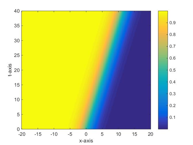
Figure 1: Example 1, desired traveling wave $u_{d}$ (left) and computed optimal state $u$ (right).

Example 2 (Stopping a traveling wave )

In contrast to Example 1, here we fix the desired pattern $u_{d}$ that is displayed in Fig. 2, left side. This desired pattern was not pre-computed but geometrically designed, i.e. it is a ”synthetic” pattern that shows a traveling wave stopping at the time $t\approx 16$. The other data are selected as in Example 1.

In the optimization process for Example 2, we fixed $\kappa=-1.5$. The initial iterate was $t_{1}=0,\,t_{2}=1$; fmincon returned $t_{1}=0.05,\,t_{2}=0.94$ as solution. The optimal state is displayed in Fig. 2.

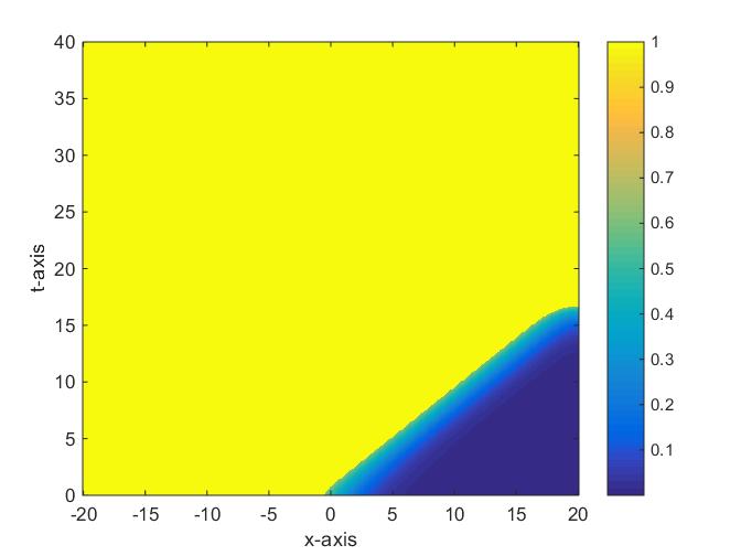
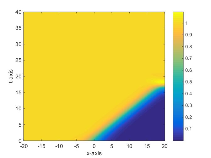
Figure 2: Example 2, synthetic desired state $u_{d}$ (left) and computed optimal state $u$ (right).

The next example shows that the applicability of the standard tracking functional $J$ of (PS) is limited to simple patterns $u_{d}$, e.g. wave type solutions of constant velocity.

Example 3 (Periodic pattern)

Also here, $u_{d}$ is a synthetic pattern that was not precomputed. In $\Omega=(-20,20)$, we define

$$u_{d}(x,t)=3\,\sin(t-\cos(\frac{\pi}{40}(x+40))).$$

Notice that this function $u_{d}$ obeys the homogeneous Neumann boundary conditions. It is displayed in Fig. 3, left. Since such a periodic pattern cannot be expected for small times, we consider the tracking only on $[T/2,T]$. Therefore, here we re-define the objective functional $J$ by

$$J_{S}(\kappa,t_{1},t_{2}):=\int_{T/2}^{T}\int_{\Omega}(u_{(\kappa,t_{1},t_{2})}-u_{d})^{2}\,dxdt+\frac{\nu}{2}(\kappa^{2}+t_{1}^{2}+t_{2}^{2}).$$

During the optimization run, we fixed the values $\kappa=-2$ and $t_{1}=0$ and optimized only with respect to $t_{2}$. Starting from $t_{2}=2$, the code fmincon returned the solution $t_{2}=3.71$. At this point, the Euclidean norm of $\nabla J_{S}$ is $|\nabla J_{S}(-2,0,3.71)|\approx 0.045$. This is a fairly good value and indicates that the result should be close to a local minimum. Nevertheless, the computed optimal objective value is very large,

$$J_{S}(-2,0,3.71)=1.32\cdot 10^{3}.$$

Remark 5

In this and in the next examples, we fix $t_{1}=0$. We observed in our computational examples that the optimization with respect to $(\kappa,t_{2})$ and $t_{1}=0$ yields sufficiently good results. Moreover, we found examples, where we got the same optimal objective value of $J$ for very different triplets $(\kappa,t_{1},t_{2})$.

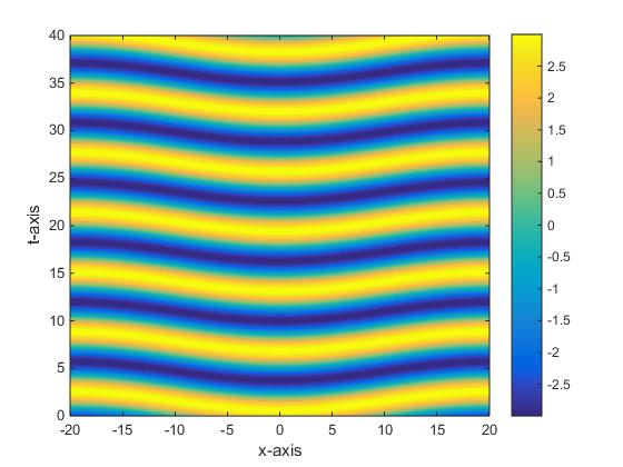
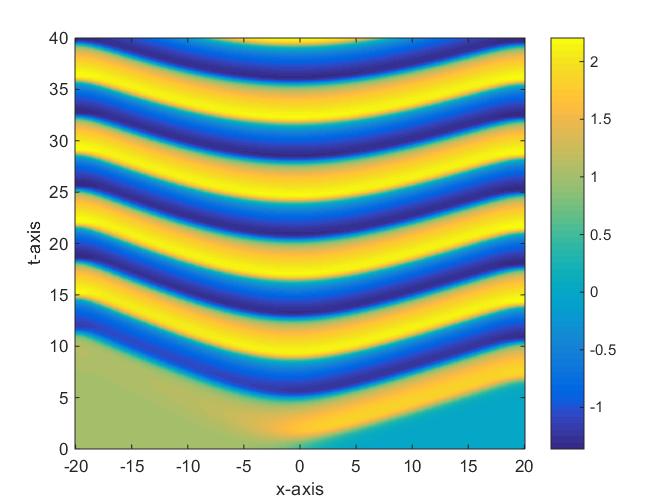
Figure 3: Example 3, Desired periodic pattern $u_{d}$ (left) and computed optimal state $u$ (right).

The computed optimal state for Example 3 is far from the desired one. In particular, the temporal periods are very different. The reason is that the standard quadratic tracking type functional $J$ is not able to resolve the desired periodicity. The main point is that the $L^{2}$-norm of the difference of a time-periodic function $t\mapsto u_{d}(t)$ and its phase shifted function $t\mapsto u_{d}(t-s)$ can be very large, although both functions have the same time period. For instance, in $Q=(-20,20)\times(0,40)$ we have

$$\iint_{Q}\left(3\sin(t-\cos(\frac{\pi}{20}(x+20)))-3\sin(t-3-\cos(\frac{\pi}{20}(x+20)))\right)^{2}dxdt=I,$$

where $I\approx 1.4374\cdot 10^{4}$. This brought us to considering another type of objective functionals that is discussed in the next section.

7 Minimizing a cross correlation type functional

The cross correlation

As Example 3 showed, we need an objective functional that better expresses our goal of approximating periodic structures. This is the cross correlation between $u$ and $u_{d}$. Moreover, in the functional, we have to observe a later part of the time interval, where $u$ already has developed its periodicity.

Let us briefly explain the meaning of the cross correlation. Assume that $x_{d}:\mathbb{R}\to\mathbb{R}$ is a periodic function and $x:[0,T]\to\mathbb{R}$ is another function; think of a function $x$ that is identical with $x_{d}$ after a time shift.

To see, if $x_{d}$ and $x$ are time shifts of each other, we consider the extremal problem

$$\min_{s\in\mathbb{R}}\int_{0}^{T}(x(t)-x_{d}(t-s))^{2}dt.$$ (38)

If $x$ and $x_{d}$ are just shifted, then the minimal value in (38) should be zero by taking the correct time shift $s$. The functional (38) can be simplified. To this aim, we expand the integrand,

$$\int_{0}^{T}(x(t)-x_{d}(t-s))^{2}dt=\int_{0}^{T}x^{2}(t)\,dt-2\int_{0}^{T}x(t)x_{d}(t-s)dt+\int_{0}^{T}x_{d}^{2}(t-s)\,dt.$$

The first integral does not depend on $s$. Since $x_{d}$ is a periodic function, also the last integral is independent of the shift $s$. Therefore, instead of minimizing the quadratic functional above, we can solve the following problem:

$$\max_{s\in\mathbb{R}}\frac{\int_{0}^{T}x(t)x_{d}(t-s)dt}{\|x\|_{L^{2}(0,T)}\|x_{d}\|_{L^{2}(0,T)}},$$ (39)

where we additionally introduced a normalization. The result is the so-called cross correlation between $x$ and $x_{d}$. The largest possible value in (39) is 1; in this case, both functions are collinear.

In the application to our control problems, this induces two equivalent objective functionals. The minimization problem (38) leads to the optimization problem

$$\min_{(\kappa,t_{1},t_{2})\in C_{\delta}}\left(\,\min_{s\in\mathbb{R}}\int_{Q}(u(x,t)-u_{d}(x,t-s))^{2}dxdt+\frac{\nu}{2}\,(\kappa^{2}+t_{1}^{2}+t_{2}^{2})\right).$$ (40)

The other way around is an equivalent problem that uses the cross correlation,

$$\min_{(\kappa,t_{1},t_{2})\in C_{\delta}}J_{corr}(\kappa,t_{1},t_{2})$$ (41)

where

$$J_{corr}(\kappa,t_{1},t_{2}):=1-\max_{s\in\mathbb{R}}\frac{\displaystyle\iint_{Q}u(x,t)u_{d}(x,t-s)dxdt}{\displaystyle\|u\|_{L^{2}(Q)}\|u_{d}\|_{L^{2}(Q)}}+\frac{\nu}{2}\,(\kappa^{2}+t_{1}^{2}+t_{2}^{2}).$$ (42)

For solving (41), we applied the Matlab code pattern search that turned out to be fairly efficient in finding global minima for functions that exhibit multiple local minima. In the periodic case, we have to deal with multiple local minima indeed. Here, the cross correlation based functional $J_{corr}$ is more useful, as the next figure shows.

Example 4 (Multiple local minima)

We pre-compute the desired state by $u_{d}=u_{(-2,0,2.5)}$ and consider the functions $\kappa\mapsto J_{S}(\kappa,0,2.5)$ and $\kappa\mapsto J_{corr}(\kappa,0,2.5)$ for $\kappa$ around the (optimal) parameter $\bar{\kappa}=-2$.

The two functions defined in Example 4 are shown in Fig. 4. The function $\kappa\mapsto J_{S}(\kappa,0,2.5)$ behaves more wildly around $\kappa=-2$ than the function $\kappa\mapsto J_{corr}(\kappa,0,2.5)$ that is based upon the cross correlation.

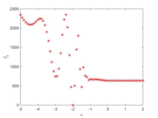
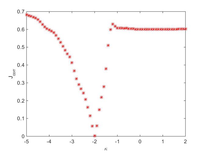
Figure 4: Example 4, goal functions $\kappa\mapsto J_{S}(\kappa,0,2.5)$ (left) and $\kappa\mapsto J_{corr}(\kappa,0,2.5)$ (right).

Let us re-consider the optimization problem of Example 3, but now by the cross correlation based optimization problem (41). Here, we apply the following strategy: We keep $t_{1}=0$ fixed and optimize only with respect to $(\kappa,t_{2})$. Moreover, at the beginning we fixed $\kappa=-2$ and optimized with respect to $\kappa$ in a second run. The computed solution was $t_{2}=2.7631$ with a value $J_{corr}=0.1604,\,(t_{1}=0,\,\kappa=-2)$; as before the Tikhonov parameter was selected as $\nu=0$. The computed $u$ of this first step is shown in Fig. 5. Now the agreement, in particular of the temporal period, is much better.

Next, we performed an alternating search for $(\kappa,t_{2})$ starting with the result obtained in the first step. We obtained $t_{2}=2.7631,\,\kappa=-2.4318$ and the improved objective value $J_{corr}=0.1229$. This improvement is graphically hardly to distinct from Fig. 5.

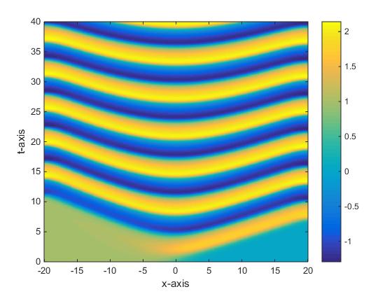
Figure 5: Example 3, Desired pattern $u_{d}$ (left) and computed pattern after minimizing $J_{corr}$ with respect to $t_{2}$ (right) for fixed $\kappa=-2,\,t_{1}=0$.

Finally, we consider another example with synthetic $u_{d}$ that has a larger period than $u_{d}$ of Example 3.

Example 5

We consider again $\Omega=(-20,20)$ and observe $u_{d}$ only in the time interval $[20,40]$. For $u_{d}$ we select

$$u_{d}(x,t)=3\,\displaystyle\sin\left(\frac{t}{2}-\cos\left(\frac{\pi}{20}(x+20)\right)\right).$$

Again, $t_{1}=0$ is fixed and the iteration is started with $t_{2}=2,\,\kappa=-2$. The optimal control parameters are $t_{2}=6.94191,\,\kappa=-2.28$ with computed optimal objective value $J_{corr}=0.1209$. The computed optimal state is shown in Fig. 6.

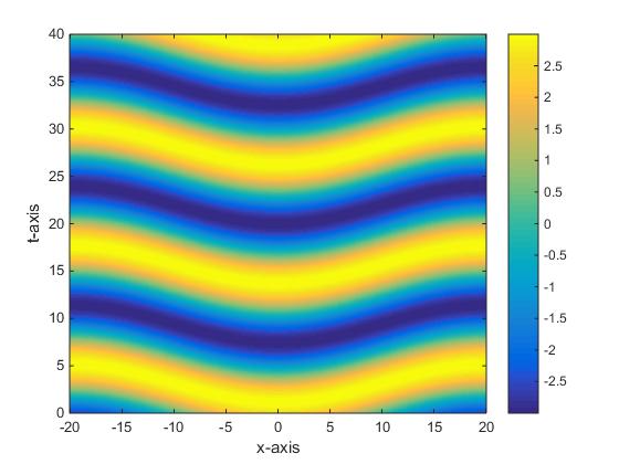
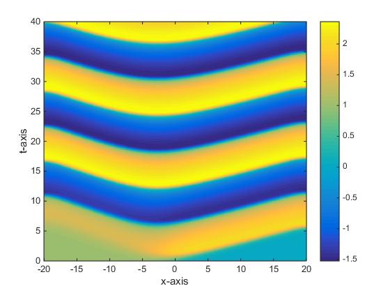
Figure 6: Example 5, desired pattern $u_{d}$ (left) and optimal pattern (right) for fixed $t_{1}=0$.

References

- (1) Atay, F.: Distributed delays facilitate amplitude death of coupled oscillators. Phys. Rev. Lett. 91, 094101 (2003)
- (2) Bachmair, C., Schöll, E.: Nonlocal control of pulse propagation in excitable media. Eur. Phys. J. B 276 (2014). DOI 10.1140/epjb/e2014-50339-2
- (3) Borzì, A., Griesse, R.: Distributed optimal control of lambda-omega systems. J. Numer. Math. 14(1), 17–40 (2006)
- (4) Brandão, A.J.V., Fernández-Cara, E., Paulo, P.M.D., Rojas-Medar, M.A.: Theoretical analysis and control results for the FitzHugh-Nagumo equation. Electron. J. Differential Equations 164, 1–20 (2008)
- (5) Buchholz, R., Engel, H., Kammann, E., Tröltzsch, F.: On the optimal control of the Schlögl model. Computational Optimization and Applications 56, 153–185 (2013)
- (6) Casas, E.: Boundary control of semilinear elliptic equations with pointwise state constraints. SIAM J. Control and Optimization 31, 993–1006 (1993)
- (7) Casas, E., Ryll, C., Tröltzsch, F.: Second order and stability analysis for optimal sparse control of the FitzHugh-Nagumo equation. Submitted (2014)
- (8) Casas, E., Ryll, C., Tröltzsch, F.: Sparse optimal control of the Schlögl and FitzHugh-Nagumo systems. Computational Methods in Applied Mathematics 13, 415–442 (2014). DOI 10.1515/cmam-2013-0016
- (9) Chamakuri, N., Kunisch, K., Plank, G.: Numerical solution for optimal control of the mono-domain equations in cardiac electrophysiology. Comput. Optim. Appl. (to appear)
- (10) Coron, J.M.: Control and Nonlinearity. American Mathematical Society, Providence (2007)
- (11) Di Benedetto, E.: On the local behaviour of solutions of degenerate parabolic equations with measurable coefficients. Ann. Scuola Sup. Pisa, Ser. I 13, 487–535 (1986)
- (12) Gugat, M., Tröltzsch, F.: Boundary feedback stabilization of the Schlögl system. Automatica (2014)
- (13) Kunisch, K., Nagaiah, C., Wagner, M.: A parallel Newton-Krylov method for optimal control of the monodomain model in cardiac electrophysiology. Comput. Vis. Sci. 14(6), 257–269 (2011)
- (14) Kunisch, K., Wagner, M.: Optimal control of the bidomain system (iii): Existence of minimizers and first-order optimality conditions. To appear in ESAIM: Mathematical Modelling and Numerical Analysis (2012)
- (15) Kunisch, K., Wang, L.: Time optimal controls of the linear Fitzhugh-Nagumo equation with pointwise control constraints. J. Math. Anal. Appl. 395(1), 114–130 (2012). DOI 10.1016/j.jmaa.2012.05.028. URL http://dx.doi.org/10.1016/j.jmaa.2012.05.028
- (16) Kyrychko, Y., Blyuss, K., Schöll, E.: Synchronization of networks of oscillators with distributed delay-coupling. Chaos 24, 043117 (2014)
- (17) Lasiecka, I., Triggiani, R.: Control Theory for Partial Differential Equations: Continuous and Approximation Theories. I: Abstract Parabolic Systems. Cambridge University Press, Cambridge (2000)
- (18) Lasiecka, I., Triggiani, R.: Control Theory for Partial Differential Equations: Continuous and Approximation Theories. II: Abstract Hyperbolic-Like Systems over a Finite Time Horizon. Cambridge University Press, Cambridge (2000)
- (19) Löber, J., Coles, R., Siebert, J., Engel, H., Schöll, E.: Control of chemical wave propagation. In: A. Mikhailov, G. Ertl (eds.) Engineering of Chemical Complexity II, pp. 185–207. World Scientific, arXiv:1403.3363, Singapore (2014)
- (20) Pyragas, K.: Continuous control of chaos by self-controlling feedback. Phys. Rev. Lett. A 170, 421 (1992)
- (21) Pyragas, K.: Delayed feedback control of chaos. Phil. Trans. R. Soc A 364, 2309 (2006)
- (22) Raymond, J.P., Zidani, H.: Pontryagin’s principle for state-constrained control problems governed by parabolic equations with unbounded controls. SIAM J. Control and Optimization 36, 1853–1879 (1998)
- (23) Raymond, J.P., Zidani, H.: Hamiltonian Pontryagin’s principles for control problems governed by semilinear parabolic equations. Applied Math. and Optimization 39, 143–177 (1999)
- (24) Schöll, E., Schuster, H.: Handbook of Chaos Control. Wiley-VCH, Weinheim (2008)
- (25) Siebert, J., Alonso, S., Bär, M., Schöll, E.: Dynamics of reaction-diffusion patterns controlled by asymmetric nonlocal coupling as a limiting case of differential advection. Physical Review E 89, 052909 (2014). DOI 10.1103/PhysRevE.89.052909
- (26) Siebert, J., Schöll, E.: Front and turing patterns induced by mexican-hat-like nonlocal feedback. Europhys. Lett. 109, 40014 (2015)
- (27) Smyshlyaev, A., Krstic, M.: Adaptive control of parabolic PDEs. Princeton University Press, Princeton, NJ (2010)
- (28) Tröltzsch, F.: Optimal Control of Partial Differential Equations. Theory, Methods and Applications, vol. 112. American Math. Society, Providence (2010)
- (29) Wille, C., Lehnert, J., Schöll, E.: Synchronization-desynchronization transitions in complex networks: An interplay of distributed time delay and inhibitory nodes. Phys. Rev. E 90, 032908 (2014)