Abstract

In this article a generalized mathematical model describing the interactions between malignant tumour and immune system with discrete time delay incorporated into the system is considered. Time delay represents the time required to generate an immune response due to the immune system activation by cancer cells. The basic mathematical properties of the considered model, including the global existence, uniqueness, non-negativity of the solutions, the stability of steady sates and the possibility of the existence of the stability switches, are investigated when time delay is treated as a bifurcation parameter. The model is validated with the sets of the experimental data and additional numerical simulations are performed to illustrate, extend, interpret and discuss the analytical results in the context of the tumour progression.

Keywords: delay differential equations, stability analysis, Hopf bifurcation, immune system, tumour, immunotherapy

1 Introduction

Cancer immunology is a new trend in immunology that focuses on the variety of interactions between the immune system and cancer cells. The aim of cancer immunology is to discover new cancer immunotherapies to fully cure or at least to retard the progression of the disease. According to recent reports [1] lymphocytes sensitive to tumour antigens are often present in the patient’s body, providing a potentially natural way to prevent tumour growth. On the other hand, it is also observed that the full immune response usually does not occur and so the natural protection afforded by the immune system is ineffective.

In general the interactions between tumour cells and immune system are very complex and involve a number of different kinds of molecules, immune cells and events, [2]. The immune response against tumour antigens involves different kinds of immune cells: B-Lymphocytes producing and secreting antibodies into the blood or placing them on their surfaces, cytotoxic T-Lymphocytes – the effector cells that destroy the antigens and thus the antigen-bearing cells, T helper-lymphocytes secreting interleukins, hence stimulate both T and B cells to divide and finally T-suppressor cells that end the immune response. All these cells are produced in the body from a small fraction of the precursor cells. Whenever antigens are presented to the precursor cells they are activated, start to proliferate and then differentiate into effector or memory cells. Unfortunately, these mechanism do not guarantee the fully efficient response of the immune system due mainly to the tumour’s own defence system. Tumour cells protect themselves from contact with lymphocytes by, amongst other methods, surface expression of ligands which initiate the apoptotic signal in the cytotoxic T-Lymphocytes, thus killing off the cytotoxic T-Lymphocytes before the necessary cell-contact with the tumour cells can be initiated.

Clearly, due to the complexity of the considered problem systems describing most of the tumour-immune system interactions would involve a large number of variables and thus equations, as in [3], where a model of 12 equations is proposed and numerically analysed or in [4], where a system of 5 equations describing the response of the effector cells to the growth of tumour cells is studied. More recently, systems of four or more equations investigating the immunotherapy and its improvement for high grade gliomas ([5, 6]), predicting outcomes of prostate cancer personalized immunotherapy ([7]) or humoral mediated immune response [8] were proposed. Also well known immune system Marchuk’s model, [9, 10, 11], describing the immune system dynamics which was applied to the description of the tumour growth phenomenon, see e.g. [12]. However, to better understand the main underlying mechanism of immune response to the presence of the tumour cells complex models were simplified and thus reduced into two- or three-equation and less detailed ones, see e.g. [13, 14, 15, 16, 17, 18, 19] or [20, 21, 22, 23, 24, 25, 26].

In this article the influence of a particular modification to the generalization of the two-equation model proposed in [19] is studied. The proposed generalization concerns the form of the stimulus function, namely only some essential assumptions regarding the shape and regularity of this function are assumed for the theoretical part of the paper. The proposed modification reflects the fact that the immune system requires some time before the presence of a tumour (actually, tumour antigens) in the body is detected and the immune system is able to respond. This assumption leads to the incorporation of a discrete time delay in the function describing the immune system stimulation by presence of the tumour cells. For the obtained system the basic mathematical properties of the model, the possible asymptotic behaviour of the system depending on the delay and the role of the native background immunity and the immune stimulation strength are investigated. For the particular form of the stimulus function the considered model is validated with two sets of the experimental data for particular tumour cell line and further studied in the context of the model dynamics within the framework of the other experimental data. It is shown that model can reflect different patterns, including periodic, reported in the experimental literature. For the estimated parameter values it is shown that an increase of the background immunity or the stimulation strength of the tumour cells on the immune system enlarge the stability region for the positive dormant steady state. Moreover, the increase of the background immunity might stabilize the unrestricted tumour growth observed for the control experiment.

The paper is organized as follows: in Section 2 the model without delay and summary of the existence and stability of the non-negative steady states are presented; in Section 3 the model with discrete delay is described and analysed. Next, in Section 4 model is validated with the experimental data. The numerical simulations confirming and extending the analytical results are shown in Section 5. Finally, in Section 6 above results are summarised and discussed.

2 Presentation of the base model

In [19] a simple model for tumour-immune system interaction, that takes into account the two most important variables: the size of specific anti-tumour immunity at time $s$ ($X(s)$) and the size of tumour ($Y(s)$), is studied. To describe the size of the overall specific immunity against the tumour Foryś et al., [19], make the following assumptions. First, in the absence of tumour antigens one observes a constant (with rate $w$) production of precursor cells that are able to respond to the tumour antigens and the natural death of the cells, which is expressed by a linear term $uX$. Thus, as a consequence of the tumour absence within the body a constant immunity level (so-called background immunity) is kept. Second, the presence of tumour antigens stimulate an increase of the immunity level. Moreover, it is assumed that immunity response is proportional to the current size of the immunity $X$ with the proportionality coefficient ($aF$), which is assumed to be a bounded function of both immunity size and tumour antigens or tumour antigens only. It is also assumed that the creation of the antibody-antigen complexes lead to the death of the immune cells and it is modelled by a bilinear term $XY$ with constant coefficient $b$. Clearly, if for particular tumours this process is not observed, then $b=0$. Finally, the destructive influence of immune system on the tumour development is described by the bilinear term $XY$ with the constant rate $c$, similarly as it was assumed in [16]. Additionally, it is assumed that the tumour grows according to the exponential law, as e.g. in [14, 20, 18], with growth rate equal to $r$. The system proposed in[19] has the following form

$$\frac{\operatorname{\mathrm{d\!}}X}{\operatorname{\mathrm{d\!}}s} =w-uX+aF(X,Y)X-bXY,$$ (2.1a)

$$\frac{\operatorname{\mathrm{d\!}}Y}{\operatorname{\mathrm{d\!}}s} =Y(r-cX),$$ (2.1b)

where the presence of tumour antigens that stimulate the immune system response ($F$) is defined by

$$F_{1}(X,Y)=\frac{Y^{\alpha}}{k_{1}^{\alpha}X^{\alpha}+Y^{\alpha}},\quad\text{or}\quad F_{2}(X,Y)=\frac{Y^{\alpha}}{k_{2}^{\alpha}+Y^{\alpha}}.$$ (2.2)

Different forms of $F_{1}$ and $F_{2}$ reflect different assumptions on tumour–immunity interactions, and both of them were earlier considered in the literature in the context of the immune system response. For $F=F_{2}$ it is assumed that the number of stimulated cells does not depend on the size of the immune system itself, hence stimulation is signal dependent. Such a form of the stimulus function in the context of immune response was considered for example in [27, 4, 28, 29] and more recently in [19, 21, 25]. In case of $F=F_{1}$ a number of signal molecules need to be reached before faster production of immune cells is activated (after which, the size of anti-tumour immunity increases) hence such a function is often called a ratio-dependent stimulation function and it was considered in the immune system - tumour interactions context in [3].

Due to the biological interpretation of constants, it is assumed that all parameters are non-negative and in particular parameters $a$, $c$, $u$, $r$, $w$ and $k_{i}$, $i=1,2$ are strictly positive. Moreover, it is assumed that $\alpha$, which describes the switching characteristics of the stimulus functions, is greater or equal to 1.

In order to simplify the model analysis, in the analytical part of the paper, its non-dimensional form is considered

$$\frac{\operatorname{\mathrm{d\!}}x}{\operatorname{\mathrm{d\!}}t} =d\big{(}\omega-x+\rho f(x,y)x-\psi xy\big{)},$$ (2.3a)

$$\frac{\operatorname{\mathrm{d\!}}y}{\operatorname{\mathrm{d\!}}t} =y(1-x),$$ (2.3b)

where $\omega=cw/(ur)>0$ is the native (background) immunity, i.e. the natural level of immunity in the absence of antigens, $\rho=a/u>0$ is the stimulation strength, $\psi=bY_{0}/u\geq 0$ ($Y_{0}=k_{1}r/c$ or $Y_{0}=k_{2}$ depending on the form of $F$ function considered) is the strength of anti-immune activity, $d=u/r>0$ and $f(x,y)$ is the stimulus function given by

$$f_{1}(x,y)=\frac{y^{\alpha}}{x^{\alpha}+y^{\alpha}}\quad\text{or}\quad f_{2}(x,y)=\frac{y^{\alpha}}{1+y^{\alpha}},\quad\alpha\geq 1,$$ (2.4)

time and variables are scaled $t=rs$ and $x=cX/r$, $y=Y/Y_{0}$, respectively.

As mentioned before in the well established literature the stimulating effect of the presence of tumour antigens on the immune system response is usually described by the function $f=f_{2}$ and often ([4, 29, 21, 25]) with $\alpha=1$ (that is by the Michaelis-Menten function). Hence, that form is considered in the part of paper devoted to the model fitting to the experimental data and its further validation. However, function $f_{2}$ given by (2.4) has several general properties, thus for the theoretical part on the paper a more general family of stimulus functions, fulfilling conditions:

1. the function $f$ is a non-negative Lipschitz continuous on $\varmathbb{R}_{\geq}=[0,+\infty)$;

2. $f(y)$ is bounded by one for all $y\in\varmathbb{R}_{\geq}$;

3. $f(0)=0$, $\lim\limits_{y\to+\infty}f(y)=1$, $f(1)=1/2$;

4. $f(y)$ is increasing for all $y\in\varmathbb{R}_{\geq}$;

5. $f(y)$ is differentiable for all $y\in\varmathbb{R}_{\geq}$;

6. the function $f$ has at most one inflection point.

and if further needed the additional smoothness

1. $f(y)\in C^{2}$ for all $y\in\varmathbb{R}_{\geq}$,

is considered.

Clearly, assumption (A1) together with the form of the system (2.3) guarantees existence of non-negative unique solutions of (2.3) with non-negative initial condition (3.2). Additionally, the global existence of the solution is a consequence of the assumption (A2).

In [19] the importance of parameters $\omega$ (background immunity) and $\mu=\omega-1+\rho$, (so-called overall immune capacity) is stressed since both of them strongly influence the existence and the stability of the steady states. Hence, due to the biological interpretation of the parameter $\mu$ in the rest of the paper its positivity, i.e.,

$$\omega+\rho>1$$

is assumed.

Because of the form of Eq. (2.3b) all non-negative steady states are always of the form $(\zeta,0)$ or $(1,\zeta)$, where $\zeta>0$. Assumption $f(0)=0$ (see (A3)) implies that there always exists a semi-trivial steady state $A=(\omega,0)$. Clearly, the existence and number of positive steady states depends on the number of solutions of equation

$$\rho f(y)=\psi y+1-\omega.$$ (2.5)

Assumption (A6) implies that there exist at most three positive solutions of (2.5). If $\psi=0$, then due to (A3) and (A4) there exist no positive solutions of (2.5) for $\omega>1$ and there exists exactly one $y_{R}$ for $\max\{0,1-\rho\}<\omega<1$. If $\psi>0$, then the situation is more complicated. If the function $f$ has no inflection point (the assumption (A3) implies that $f$ is concave), then for $0<\omega<1$ Eq. (2.5) has zero or two solutions in a generic case. On the other hand, for $\omega>1$ Eq. (2.5) has exactly one positive solution. If the function $f$ has one inflection point, Eq. (2.5) has one or three positive solutions for $\omega>1$ and zero or two for $0<\omega<1$ (in a generic case).

Arguments analogous to those presented in [19] imply that the stability of the steady states of the system (2.3) with $f$ fulfilling conditions (A1)-(A6) are the same as for particular forms of $f$ functions given by (2.4). The results regarding the existence and stability of the steady states of (2.3) are summarized in Tab. 1 and partially in Fig. 1. Note that, in [19] additionally it is shown that there are no periodic solutions of the system (2.3).

Table 1: Existence and stability of the steady states of the system (2.3) for $f$ fulfilling conditions (A1)–(A6) depending on values of parameters $\alpha,\omega,\psi,\rho$. Numbers in the column ips indicate the number of possible inflection points of the function $f$.

$\psi$	$\omega$	ips	Steady states	Stability
Semi-trivial steady states
$\psi\geq 0$	$0<\omega<1$	$0,1$	$A=(\omega,0)$	unstable
	$\omega>1$			locally stable
Positive steady states
$\psi=0$	$0<\omega<1^{*}$	$0,1$	$R=(1,y_{R})$, $y_{R}>0$	globally stable
	$\omega>1$		none
$\psi>0$	$0<\omega<1$	$0,1$	none
			$B=(1,y_{B}),\,\,C=(1,y_{C})$	$B$ locally stable
			$0<y_{B}<y_{C}$	$C$ unstable
	$\omega>1$	$0,1$	$C=(1,y_{C})$, $y_{C}>0$	$B$ unstable
		$1$	$B=(1,y_{B}),\,\,C=(1,y_{C}),\,\,D=(1,y_{D})$	$B$ unstable
			$0<y_{B}<y_{C}<y_{D}$	$C$ locally stable
				$D$ unstable

^∗ under assumption $\omega+\rho>1$

Since in a later section of the paper $f$ is given by the Michaelis-Menten function, the conditions for the existence of positive steady states of the system (2.3) for $\alpha=1$ and $f=f_{2}$ are directly provided below (compare with Figure 1).

Proposition 2.1

Let $\psi=0$ and $f=f_{2}$ is given by (2.4), then

1. for $\omega>1$ there are no positive steady states of the system (2.3);

2. for $\max\{0,1-\rho\}<\omega<1$ there is exactly one positive steady state of the system (2.3) given by

   $$R=(1,y_{R})=\left(1,\Big{(}\frac{1-\omega}{\rho+\omega-1}\Big{)}^{\frac{1}{\alpha}}\right).$$

Proof : Because of the form of Eq. (2.3b) all positive steady states are always of the form $(1,\zeta)$, where $\zeta>0$. Clearly, the existence and number of positive steady states depends on the number of solutions of (2.5). For $\psi=0$, due to the facts: $f(0)=0$, $\lim\limits_{y\to+\infty}f(y)=1$ and $f$ being increasing, there exist no positive solutions of (2.5) for $\omega>1$ and there exists exactly one $\zeta$ for $\max\{0,1-\rho\}<\omega<1$.  

Proposition 2.2

Let $\psi>0$, $\alpha=1$, $f=f_{2}$ is given by (2.4) and $\Delta=\left(1+(1-\omega-\rho)/\psi\right)^{2}-4(1-\omega)/\psi$, then

1. for $\omega>1$ there exits a unique positive steady state $C=(1,y_{C})$ of the system (2.3) with

   $$y_{C}=\frac{1}{2}\left(\frac{\rho+\omega-1}{\psi}-1+\sqrt{\Delta}\right).$$ (2.6)

2. for $0<\omega<1$ and $\rho>\bigl{(}\sqrt{\psi}+\sqrt{1-\omega}\bigr{)}^{2}$ two positive steady states $(1,y_{B})$ and $(1,y_{C})$ of the system (2.3) exist where

   $$y_{B}=\frac{1}{2}\left(\frac{\rho+\omega-1}{\psi}-1-\sqrt{\Delta}\right)$$

   and $y_{C}$ is given by (2.6). On the other hand, if $0<\omega<1$ and $\rho<\bigl{(}\sqrt{\psi}+\sqrt{1-\omega}\bigr{)}^{2}$, then there are no positive steady states of the system (2.3).

Proof :

Eq. (2.5) takes form $\rho y=\Bigl{(}\psi y+1-\omega\Bigr{)}\bigl{(}1+y\bigr{)}$. Dividing both sides by $\psi$ and denoting $\beta=\frac{1-\omega}{\psi}$ and $\nu=\frac{\rho}{\psi}$ one obtains

$$y^{2}+(1-\nu+\beta)y+\beta=0.$$ (2.7)

Inequality $\omega>1$ implies $\beta<0$, hence Eq. (2.7) has one positive solution and the part (i) follows.

For $0<\omega<1$ there is $\beta>0$. If real roots of (2.7) exist, then they have the same sign. Moreover, they are positive if and only

$$\nu>1+\beta.$$ (2.8)

On the other hand, the existence of real solutions to (2.7) depends on the sign of the determinant $\Delta=(1-\nu+\beta)^{2}-4\beta=\nu^{2}-2\nu(1+\beta)+(1-\beta)^{2}$. It can be easily calculated that $\Delta>0$ if and only if

$$\nu<\bigl{(}1-\sqrt{\beta}\bigr{)}^{2}\quad\text{ or }\quad\nu>\bigl{(}1+\sqrt{\beta}\bigr{)}^{2}.$$ (2.9)

Note, that for $\beta>0$ the first inequality of (2.9) is equivalent to $\nu<1+\beta-2\sqrt{\beta}$, which contradicts (2.8). On the other hand, the second inequality of (2.9) is equivalent (again for $\beta>0$) to $\nu>1+\beta+2\sqrt{\beta}$, which implies (2.8). Thus, the part (ii) follows.  

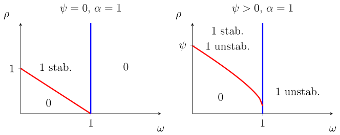
Figure 1: The $\omega-\rho$ space divided into regions where different numbers of steady states for $\alpha=1$ and $\psi=0$ or $\psi>0$ are observed. Numbers and text in the regions indicate the number of positive steady states of the system (2.3) for $f=f_{2}$ and theirs stability for $\tau=0$; abbreviations stab. and unstab. stand for stable and unstable, respectively.

3 Model with discrete time delay

The immune system requires some time before the presence presence of the tumour (or rather, the tumour’s antigens) in the organism is detected and the immune system is able to respond. From the mathematical point of view, to reflect such phenomena, one can include time lags into the system, e.g. by introducing a discrete delay into the stimulus function. Although the model itself differs from the one considered in [21], the idea presented there of introducing one discrete time delay only in the function describing the stimulating effect of the tumour on immune cells proliferation in the system variable representing the tumour cells compartment is followed here. That assumption reflects situation when the immune system response due to the presence of the tumour cells depends on the amount of the immune system cells at a given time $t$ and on the amount of tumour cells at time $t-\tau$, where $\tau>0$ is the time needed for the immune system to develop a suitable response after antigens recognition. Following that approach time lag is introduced in a classical way, as it is done in the logistic model by Hutchinson [30] or in the Gompertz model [31, 32], where delay is introduced to the function representing the per capita growth rate. The same assumption of the form of time delay in the model of the immune system-tumour interactions has been recently made e.g. in [24]. Clearly, in the literature [15, 17, 18] discrete delay in the variable representing the size of the immune system was also considered. However, this idea is not followed since the priority is given to the immune system’s time reaction. It is also assumed that the immune system does not require time to know the size of itself.

The non-dimensional system with one discrete delay has the following form

$$\frac{\operatorname{\mathrm{d\!}}x(t)}{\operatorname{\mathrm{d\!}}t} =d\big{(}\omega-x(t)+\rho f(y(t-\tau))x(t)-\psi x(t)y(t)\big{)},$$ (3.1a)

$$\frac{\operatorname{\mathrm{d\!}}y(t)}{\operatorname{\mathrm{d\!}}t} =y(t)(1-x(t)),$$ (3.1b)

where function $f$ fulfils conditions (A1)-(A6) (and (A7) if needed).

To close system (3.1) one needs to define the initial condition

$$x(t)=\varphi_{1}(t),\quad y(t)=\varphi_{2}(t),\,\,\text{for }t\in[-\tau,0],\quad\varphi_{1}(t),\varphi_{2}(t)\in\mathcal{C},$$ (3.2)

where $\mathcal{C}=\mathbf{C}\left([-\tau,0],\mathbb{R}_{\geq}\right)$ denotes the set of continuous functions defined on the interval $[-\tau,0]$ with non-negative values. Clearly, since in system (3.1) only $y$ variable has delayed argument model dynamics will depend on $\varphi_{1}(0)$ and $\varphi_{2}(t)$.

Theorem 3.1

Let $f$ fulfils assumptions (A1)-(A2), then there exists a global, unique and non-negative solution of system (3.1)-(3.2).

Proof : For $t\in[0,\tau]$ $y(t-\tau)=\varphi_{2}(t-\tau)\geq 0$ is well defined thus for $\varphi_{1}(t),\varphi_{2}(t)\in\mathcal{C}$, under assumption (A1), there exists an interval $[0,t^{*})\subset[0,\tau]$ where the solution $(x(t),y(t))$ of the system  (3.1) exists and is unique, for details see [33].

Re-writing Eq. (3.1b) in the integral form ($y(t)=\varphi_{2}(0)\exp{\int_{0}^{t}(1-x(s))ds}$) one obtains non-negativity of $y(t)$ whenever it exists. Now, assume that at point $t_{1}\in(0,t^{*})$ $x(t)$ starts to be negative, i.e. $x(t)>0$ for $0<t<t_{1}$, $x(t_{1})=0$ and $\dot{x}(t_{1})\leq 0$. Clearly, for considered $f(y)$ inequality $\dot{x}(t_{1})=d\big{(}\omega-x(t_{1})+\rho f(y(t_{1}-\tau))x(t_{1})-\psi x(t_{1})y(t_{1})\big{)}=d\omega>0$, holds. That contradicts the hypothesis that solution $x(t)$ starts to be negative for $t=t_{1}$.

On the other hand, the non-negativity of $x(t)$ and $y(t)$ imply $y(t)\leq\varphi_{2}(0)e^{t^{*}}$. Moreover, stimulus function $f(y)$ fulfils assumptions (A1)-(A2). Hence, $\dot{x}\leq d(\omega+\rho x)$ and $x(t)\leq e^{d\rho t^{*}}\left(\varphi_{1}(0)+\frac{\omega}{\rho}\right)-\frac{\omega}{\rho}$. Thus, both variables and theirs derivatives are bounded, so the solution can be extend through the point $t^{*}$. Following the method of steps (see e.g. [33]) and repeating presented arguments for each interval $[n\tau,(n+1)\tau]$, $n\in\mathbb{N}$ one completes the proof.     

3.1 Stability of the steady states

Clearly, the steady states of the system with delay (3.1) are the same as for the system without delay (2.3). However, the system’s stability, already strongly depending on the values of parameters $\phi$ and $\omega$ without delay, now can also depend on the value of parameter $\tau$.

Theorem 3.2

Let $f$ fulfils conditions (A1)–(A5). The semi-trivial steady state $A=(\omega,0)$ of system (3.1)-(3.2) is a locally stable node for $\omega>1$ and a saddle for $\omega<1$ independently of the value of parameter $\tau\geq 0$.

Proof : For $\tau=0$ steady state $A$ is a locally stable node (for $\omega>1$) or a saddle (for $0<\omega<1$) and it always exists, for details see [19]. Consider $\tau>0$. Linearising system (3.1) around steady state $A$ one obtains system without delay which is the same as the linearisation of the system (2.3) without delay. Hence, parameter $\tau$ has no influence on the local stability of semi-trivial steady state $A$.     

As pointed earlier, for all positive steady states the first coordinate equals to 1, thus $(1,\zeta)$, $\zeta>0$ denotes the positive steady state of the system (3.1). Moreover, to simplify the notation define

$$\gamma_{f}:=\rho f^{\prime}(\zeta)=\rho\frac{\alpha\zeta^{\alpha-1}}{(1+\zeta^{\alpha})^{2}}>0,$$ (3.3)

which is positive due to the assumption (A4).

Theorem 3.3

Let $f$ fulfils conditions (A1)–(A7), $\psi\geq 0$ and $\gamma_{f}>0$ is given by (3.3).

1. If $\psi-\gamma_{f}>0$, then the steady state $(1,\zeta)$ of system (3.1) is unstable for all $\tau\geq 0$.

2. If $\psi-\gamma_{f}<0$, then the steady state $(1,\zeta)$ of system (3.1) is locally asymptotically stable for $\tau=0$ and there exists a critical value $\tau_{cr}^{\zeta}$ such that $(1,\zeta)$ is locally asymptotically stable for $\tau<\tau_{cr}^{\zeta}$ and is unstable for $\tau>\tau_{cr}^{\zeta}$. Moreover, for $\tau=\tau_{cr}^{\zeta}$, the Hopf bifurcation occurs and periodic solutions arise with period equal to $2\pi/\sqrt{\eta^{\zeta}}$ , where

   $$\eta^{\zeta}=\frac{-(2d\zeta\psi+(d\omega)^{2})+\sqrt{(d\omega)^{4}+4d^{3}\zeta\psi\omega^{2}+4(d\zeta\gamma_{f})^{2}}}{2},\quad\tau_{cr}^{\zeta}=\frac{1}{\sqrt{\eta^{\zeta}}}\arccos{\left(\frac{\eta^{\zeta}+d\zeta\psi}{d\zeta\gamma_{f}}\right)}.$$ (3.4)

Proof : Linearising system (3.1) around steady state $(1,\zeta)$ one obtains

$$\frac{\operatorname{\mathrm{d\!}}x(t)}{\operatorname{\mathrm{d\!}}t}=d(-1+\rho f(\zeta)-\psi)x(t)-d\psi y(t)+\rho\gamma_{f}y(t-\tau),\quad\quad\frac{\operatorname{\mathrm{d\!}}y(t)}{\operatorname{\mathrm{d\!}}t}=-\zeta x(t).$$

Note that for steady state $(1,\zeta)$ equality $1-\rho f(\zeta)+\psi\zeta=\omega$, holds. Thus, the characteristic function for each positive steady state $(1,\zeta)$ has the following form

$$W(\lambda)=\lambda^{2}+d\omega\lambda-d\psi\zeta+d\zeta\gamma_{f}\operatorname{\mathrm{e}}^{-\lambda\tau}.$$ (3.5)

Clearly, for $\tau=0$ Eq. (3.5) reads $W(\lambda)=\lambda^{2}+d\omega\lambda-d\zeta(\psi-\gamma_{f})$ and for $\psi-\gamma_{f}>0$ it has two real solutions of opposite signs. Thus, in such a case steady state $(1,\zeta)$ is a saddle. On the other hand, for $\tau=0$ and $\psi-\gamma_{f}<0$ both roots are real and negative or complex with negative real parts, hence $(1,\zeta)$ is locally asymptotically stable. From the continuous dependence, one knows that for sufficiency small delays this result holds, however, the stability of the steady state(s) might change for a larger values of delay, see e.g. [33]. Such a situation is only possible if there exists a critical value $\tau=\tau_{cr}^{\zeta}$ and a pair of purely imaginary roots of (3.5) such that roots cross the imaginary axis (in the proper direction) when $\tau$ exceeds $\tau_{cr}^{\zeta}$.

Let $\pm i\theta$ be a pair of pure imaginary roots of (3.5). Hence, $W(i\theta)=-\theta^{2}+id\omega\theta-d\zeta\psi+d\zeta\gamma_{f}\big{(}\cos{\theta\tau}-i\sin{\theta\tau}\big{)}=0$, and

$$\cos{\theta\tau}=\frac{\theta^{2}+d\psi\zeta}{d\zeta\gamma_{f}}>0,\quad\sin{\theta\tau}=\frac{d\omega\theta}{d\zeta\gamma_{f}}>0.$$ (3.6)

A solution of system (3.6) exists if condition $d\zeta(\psi-\gamma_{f})\leq-\theta^{2}$ is fulfilled. Hence, for $\psi-\gamma_{f}>0$ the characteristic quasi-polynomial (3.5) of the system (3.1) has no purely imaginary roots and hence the real parts of eigenvalues can not change sign for any value of $\tau\geq 0$. That completes the proof of part 1.

Consider $\psi-\gamma_{f}<0$. Squaring and adding Eqs. (3.6) one has

$$\tilde{F}(\theta):=\theta^{4}+d\Bigl{(}2\psi\zeta+d\omega^{2}\Bigr{)}\theta^{2}+d^{2}\zeta^{2}\Bigl{(}\psi^{2}-\gamma_{f}^{2}\Bigr{)}=0.$$ (3.7)

Next, substituting $\eta=\theta^{2}$ one gets $\eta^{2}+\eta((d\omega)^{2}+2d\zeta\psi)+(d\zeta)^{2}(\psi^{2}-\gamma_{f}^{2})=0$ with roots given by

$$\eta_{1,2}^{\zeta}=\frac{-(2d\zeta\psi+(d\omega)^{2})\pm\sqrt{(2d\zeta\psi+(d\omega)^{2})^{2}-4(d\zeta)^{2}(\psi^{2}-\gamma_{f}^{2})}}{2}.$$ (3.8)

Clearly, roots (3.8) are always real since the expression $(2d\psi\zeta+(d\omega)^{2})^{2}-4(d\zeta)^{2}(\psi^{2}-\gamma_{f}^{2})$ is strictly positive for $\psi-\gamma_{f}<0$. Moreover, for $\psi-\gamma_{f}<0$ roots have opposite signs. Denote the positive root by $\eta_{1}^{\zeta}>0$, then there exists $\bar{\theta}^{\zeta}=\sqrt{\eta_{1}^{\zeta}}$ such that $0<(\bar{\theta}^{\zeta})^{2}+2d\zeta\psi<d\zeta\gamma_{f}$, and moreover $W(i\bar{\theta}^{\zeta})=0$ for an infinite sequence of critical values of $\tau$ given by

$$\tau_{cr,k}^{\zeta}=\frac{1}{\bar{\theta}^{\zeta}}\left(\arccos{\left(\frac{\left({\bar{\theta^{\zeta}}}\right)^{2}+2d\zeta\psi}{d\zeta\gamma_{f}}\right)}+2k\pi\right),\quad k\in\mathbb{N}_{0}.$$ (3.9)

Denote by $\tau_{cr}^{\zeta}$ the first positive delay fulfilling condition (3.9). To complete the proof one needs to show that the real part of eigenvalues of roots cross the imaginary axis at $\tau=\tau_{cr}^{\zeta}$ with positive speed, i.e. $\frac{\partial}{\partial\tau}\textrm{Re}{\lambda(\tau)}|_{\tau=\tau_{cr}^{\zeta}}>0$ and that the re-stabilization of the positive steady state is not possible for larger values of $\tau$. Here, using the theorem proved by Cooke and Van den Driessche in [34], one can show that all the roots of the characteristic quasi-polynomial (3.5) cross the imaginary axis from the left to the right-hand side of the complex plane. The Cooke and Van den Driessche theorem indicates that $\frac{\partial}{\partial\tau}\textrm{Re}{\lambda(\tau)}|_{\tau=\tau_{cr,k}^{\zeta}}=\frac{d\widetilde{F}(\theta)}{d\theta}|_{\eta=\bar{\eta}^{cr}}$, hence it is enough to calculate $\frac{d\widetilde{F}(\theta)}{d\theta}=4\theta^{3}+2d\theta(2\psi\zeta+d\omega^{2})>0$ for $\theta>0$. Thus, in the case when the steady state is locally asymptotically stable for $\tau=0$, for $\tau=\tau_{cr}^{\zeta}$ new periodic orbits arise due to the Hopf bifurcation with period equal to $2\pi/\bar{\theta^{\zeta}}$. Moreover, destabilized steady state $(1,\zeta)$ remains unstable for all $\tau>\tau_{cr}^{\zeta}$. That completes the proof.     

4 Experimental data, estimation of parameters and model validation

The model parameters are obtained by fitting the solutions of the non-scaled version of model (3.1) to the experimental data provided in [35] for mice affected by B-cell lymphoma in the spleen (BCL₁). It is assumed that $F$ is given by the Michaelis-Menten function ($F=F_{2}$ defined by (2.2) with $\alpha=1$) since it is the most common form of the stimulation function considered in that context in the literature, see e.g. [4, 29, 21, 25]. Estimation of the ranges for each parameter is based on the experimental literature as well as on the assumptions made by other scientists who in particular modelled the BCL₁ and DLBCL (diffuse large B-cell lymphoma) progression or modelled the tumour-immune system interactions in general [4, 25, 36, 29, 18, 13].

4.1 Experimental data

The solutions to non-scaled version of model (3.1) are fitted to the experimental data for BCL₁ from [35], where the modelled experiment was performed on two sets of animals: the control group (BALB/c mice) and chimeric. Chimeric animals were obtained from BALB/c mice by having, by lethal irradiation, their bone marrow destroyed and then having bone marrow transferred from other mice to rebuild the immune system. In normal BALB/c mice, one observes that $5\times 10^{5}$ injected BCL₁ cells into the spleens grew rapidly, reaching a plateau after 40 days and causing mice death by 90 days. In contrast, identically injected groups of chimeric animals demonstrated a different growth pattern: the initial rate of growth was similar to the control group, but then it slowed down with tumours reaching their maximum sizes (10 times smaller than in control mice) and a commensurate decrease in the number of cells was observed after day 40, see Figure 2.

4.2 Parameter ranges

Tumour growth rate ($r$). Tumour volume duplication time strongly depends on the tumour type. For some tumours it can be 20 days, while for others, e.g. colon cancer, it can be years. On the other hand, the tumour doubling time for malignant lymphoma is reported to be around 29 days, [37]. In [36], for DLBCL, it was assumed that the tumour doubling time is between 1.4 and 70 days which corresponds to a tumour growth rate between 0.0099 and 0.4951 day^-1 (approximately 0.01 and 0.5 day^-1). That assumption is followed since the interval [0.01,0.5] includes the range 0.05-0.5 proposed in [25]. Clearly, the tumour growth rate estimated by Kuznetsov et al. in [4] (0.18 day^-1) also lies in that interval.

Natural lymphocyte death rate ($u$). The mean lifetime of T lymphocytes from the spleen and the blood was estimated to be approximately 30 days or more, [38]. Thus, the degradation rate, which is 1/(mean life time), is assumed to be in the range $1.25\times 10^{-2}-5\times 10^{-2}$ day^-1, which corresponds to $20-80$ days mean life time. The values of the death rate $0.03125$ and $0.0412$ day^-1 estimated in [25] and [4], respectively, also lie in the assumed range.

Immune response function ($F$, $\alpha$, $k_{2}$, $a$). It is assumed that the immune system response term has the same form as those considered e.g. in [4, 13, 29, 21, 25] or [36], that is $F=Y^{\alpha}/(k_{2}^{\alpha}+Y^{\alpha})$ with $\alpha=1$. In [4] the value of the steepens of the immune response function ($k_{2}$) was estimated to be $2.019\times 10^{7}$ cells, while in [25] the value $1.5109\times 10^{7}$ cells. In this study the range of $10^{7}-2\times 10^{8}$ cells for $k_{2}$ is chosen. To determine the range of the maximal immune system response rate ($a$) [25] is followed and range 0-2.5 day^-1, which contains the value $0.1245$ day^-1 estimated in [4], is taken.

Tumour independent production rate of effector cells ($w$). Following [25] the range for the constant influx of effector cells ($w$) from the immune system in the absence of tumour is chosen to be $3.2\times 10^{3}-3.2\times 10^{4}$ cells day^-1. The value $1.3\times 10^{4}$ cells day^-1 estimated by [4] belongs to the considered range.

Tumour-induced inactivation rate of effector cells ($b$). In [25] the range for the fraction of immune cells inactivated due to the interactions with tumour cells ($w$) was assumed to be $10^{-12}-5\times 10^{-7}$ cells^-1 day^-1. The value $3.422\times 10^{-10}$ cells^-1 day^-1 estimated in [4] belongs to the assumed range.

Effector induced elimination rate of tumour cells (c). In [18] the range for the fraction of cancer cells killed per effector cell was assumed to be $10^{-9}-10^{-7}$ cells^-1day^-1. However, in [4] the value of that parameter was estimated to be equal to $1.101\times 10^{-7}$ cells^-1day^-1. Hence, the range is extended and it is assumed to be $c\in[10^{-9},3\times 10^{-7}]$.

Time delay in the immune system activation ($\bar{\tau}$). In this study it is assumed that time delay in immune system response is in range from 1h till 5 days, i.e. 0.0416-5 days.

All ranges of the model parameters together with corresponding references are given in Table 2.

Table 2: Parameter ranges with referenced used for the fitting procedure to the experimental data from [35].

Par.	Biological interpretation	Unit	Range	Reference
$w$	tumour independent production rate of effector cells	cells day-1	$3.2\times 10^{3}-3.2\times 10^{4}$	[25], [4]
$u$	natural lymphocyte death rate	day-1	$1.25\times 10^{-2}-5\times 10^{-2}$	[38] [25], [4].
$a$	maximal immune response rate	day-1	0-2.5	[25], [4]
$b$	fraction of immune cells inactivated in interactions with tumour cells	cells-1 day-1	$10^{-12}-5\times 10^{-7}$	[25], [4]
$r$	tumour growth rate	day-1	$0.01-0.5$	[36], [25], [4], [37]
$c$	fraction of cancer cells killed per effector cell	cell-1 day-1	$10^{-9}-3\times 10^{-7}$	[18], [4]
$\bar{\tau}$	time delay	day	$0.0416-5$	ass.
$k_{2}$	steepens of immune response	cells	$10^{7}-2\times 10^{8}$	[25],[4]
$\alpha$	detrmines type of immune response	–	1	[4], [13], [29], [21], [25], [36]

4.3 Estimation of model parameters

Clearly, if there are no tumour cells in the system ($Y=0$), then immune-activity stays at the constant level calculated directly from (2.1a). Hence, the initial condition for the variable $X$ is a constant equal to $w/u$. On the other hand, to determine the level of the tumour cells at the beginning of the experiment (at $s=0$) one can directly use the data from [35] taking $\Phi_{2}(0)=5\times 10^{5}$ cells. Thus, the initial condition for non-scaled version of (3.1) reads

$$\Phi_{1}(s)=\frac{w}{u}\,\,\,\textrm{for}\,\,\,s\in[-\bar{\tau},0],\quad\textrm{and}\quad\Phi_{2}(s)=\begin{cases}0&\textrm{for}\,\,\,s\in[-\bar{\tau},0),\\ 5\times 10^{5}&\textrm{for}\,\,\,s=0,\end{cases}$$ (4.1)

and due to the dependencies on the parameters $w$, $u$ and $\bar{\tau}=\tau/r$ the initial condition is estimated within the fitting procedure.

The fitting procedure is performed in the commercial MATLAB^® computational environment using the PSO function. PSO finds a minimum of a function of several variables using the particle swarm optimization algorithm based on the stochastic optimization technique that was inspired by the social behaviour of bird flocking or fish schooling. The algorithm was originally introduced in 1995 by Kennedy and Eberhart, [39], and later extended by Shi and Eberhart, [40]. Nowadays it has a number of extensions, however the main idea is the same a swarm of particles moves around in the search space and the movements of the individual particles are influenced by the improvements discovered by the others in the swarm. In [41] Clerc and Kennedy introduced a constriction factor in PSO, which was later shown to be superior to the inertia factors. That version of algorithm is used here. Solutions of delay differential equations (DDEs) are computed using dde23 function with tolerance RelTol =1e-7, and AbsTol=1e-11.

In the presented study the objective function is the standard one based on the calculation of mean square error (MSE):

$$\textrm{MSE}=\frac{1}{m}\sum_{i=1}^{m}err_{i}^{2},\quad\quad err_{i}=\frac{x^{data}_{i}-x^{sym}_{i}}{x^{data}_{i}},$$

where $m$ is the number of experimental measurements, $x^{data}_{i}$ are the measured values and $x^{sym}_{i}$ are the values of the solution of DDEs for respective time points.

Table 3: Fitted non-scaled model parameters, steady states and theirs stability for $\bar{\tau}=0$ for non-scaled system (3.1). Parameter $\alpha$=1.

	control	chimeric
parameters
$w$	$3.0337\times 10^{4}$
$u$	$0.0196$
$a$	$0.1452$	$0.2835$
$k_{2}$	$1.3604\times 10^{8}$	$1.8720\times 10^{8}$
$b$	$2.1010\times 10^{-10}$	$6.6828\times 10^{-10}$
$r$	0.4695
$c$	$1.7608\times 10^{-7}$	$2.0761\times 10^{-7}$
$\bar{\tau}$	$3.1869$	$0.0581$
steady states and theirs stability for $\bar{\tau}=0$
semi trivial unstable	$(1.5472\times 10^{6},0)$	$(1.5472\times 10^{6},0)$
positive stable	$(2.6666\times 10^{6},1.0548\times 10^{7})$	$(2.2616\times 10^{6},7.8919\times 10^{6})$
positive unstable	$(2.6666\times 10^{6},5.0530\times 10^{8})$	$(2.2616\times 10^{6},2.1986\times 10^{8})$

Table 4: Fitted model parameters for system (3.1), parameter $\alpha$=1.

	$d$	$\omega$	$\rho$	$\psi$	$\tau$
control	$0.0418$	$0.5802$	$7.4046$	$1.4576$	$1.4964$
chimeric		$0.6841$	$14.4583$	$6.3802$	$0.0273$

Table 5: Summary of the bifurcation phenomena for scaled parameters given in Table 4 and $\tau$ treated as a bifurcation parameter, $\alpha=1$.

Param. type	steady state	stability $\tau=0$	$\tau_{cr}$	period	bif. type
control	(0.5802, 0)	unstable	unstable for $\tau\geq 0$
	(1, 0.0775)	stable	1.1776	50.1363	supercritical
	(1, 3.7145)	unstable	unstable for $\tau\geq 0$
chimera	(0.6841, 0)	unstable	unstable for $\tau\geq 0$
	(1, 0.0422)	stable	1.2227	57.3715	supercritical
	(1, 1.1745)	unstable	unstable for $\tau\geq 0$

First, the solutions of the non-scaled version of system (3.1) are fitted to the data from the chimera experiment for BCL₁ tumour cell population in the spleen of the BALB/c mice over 110 days (described in [35]) with the initial condition given by (4.1) that depends on $w$, $u$ and $\bar{\tau}$ parameter values. The result of the fitting procedure is presented in Figure 2 (left) showing a good agreement with the experimental data (with MSE at the level of $3.57\%$) and thus positively validates the proposed model.

Next, the parameters $w$, $u$ and $r$ are fixed (as for chimera experiment) and the rest of the parameters are fitted to the 90 day control mice experiment to further validate the model. This time a very good agreement with the experimental data with MSE at the level of $0.14\%$ is obtained, see Figure 2 (right). The corresponding values of the estimated parameters for both experiments are given in Table 3.

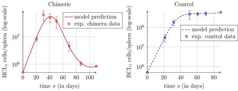
Figure 2: (Left) Result of the fitting procedure of the trajectories of the non-scaled version of system (3.1) to the experimental data for BCL₁ tumour cell population in the spleen of the chimeric mice over 110 days experiment described in [35]. MSE=0.0357. (Right) Result of the fitting procedure of the trajectories of the non-scaled version of system (3.1) to the experimental data for BCL₁ tumour cell population in the spleen of the BALB/c mice over 90 days control experiment described in [35]. MSE=0.0014. In both panels solutions of the non-scaled version of system (3.1) are computed with RelTol=1e-7 and AbsTol=1e-11. All used parameter values, for both panels, are given in Table 3. Bars indicate the measurement errors as reported in [35].

5 Results

Comparing the sets of parameters (see Table 3) for both experiments estimated via the fitting procedures one immediately sees that for the chimeric set of parameters parameter $a$ is two times larger than for the control set. Thus, together with slightly larger $k_{2}$ (for the chimeric experiment) implies a stronger stimulation of the immune system due to the presence of the tumour cells. Additionally, the time lag of that response is much shorter, approx. 1.4 h, for the chimeric set of parameters than for the control, approx. 76.5 h, indicating a more effective immune system reaction in the presence of the tumour cells for the chimeric mice. For both the chimeric and control sets, the estimated value of the tumour cells killed per effector cells $(c)$ is very similar. Despite the large range for parameter $b$ ($10^{-12}-5\times 10^{-7}$, see Table 2) and that no further assumptions on the range of $b$ to differentiate the chimeric and control experiments are made, the fitted values obtain the same order of magnitude.

The simulations presented in Figure 3 again validate positively the model and confirm results from [35] showing that for larger than control initial injection of populations of the tumour BCL₁ cells into the spleens of the chimeric mice leads to the same growth pattern. Experiments performed in [35] indicate that even if one injects $5\times 10^{7}$ cells after around 110 days, due to the immune system response, the number of tumour cells is reduced to the almost the same amount as for $5\times 10^{5}$ initially injected cells. To reproduce that phenomena all used parameter values were fixed, as given in Table 4 (column chimeric) and only a part of the initial condition that is $\Phi_{2}(0)$ was changed, see Figure 3.From the mathematical point of view such behaviour shows that the stable steady state, that can be identified as a dormant tumour state, has large enough basin of attraction.

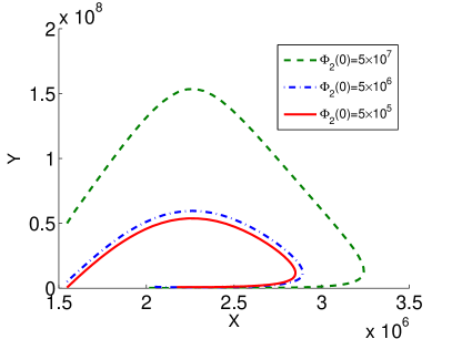
Figure 3: Trajectories of the non-scaled version of tumour-immune system (3.1) for initial condition as defined in (4.1) with different values of $\Phi_{2}(0)$: $5\times 10^{5}$ (dash green line), $5\times 10^{6}$ (dash-dot blue line) and $5\times 10^{7}$ (solid red line). All used parameter values are given in Table 3 (column chimeric), $s\in[0,110]$. All solutions computed with RelTol=1e-7 and AbsTol=1e-11.

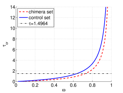
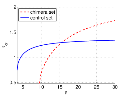
Figure 4: (Left) Critical values of the bifurcation parameter as the functions of $\omega$ (left) and as the functions of $\rho$ (right) for both chimeric (red dash line) and control (blue solid line) sets of parameters. All used parameter values (except $\omega$, $\rho$ and $\tau$) are given in Table 4. The stability regions lie below the solid blue and the dashed red lines. The horizontal grey dash-dot line in the left panel indicates the value of delay estimated via the fitting procedure for the control experiment $\tau=1.4964$.

For the sets of estimated parameters that have been scaled and are given in Table 4 the system (3.1) has one semi-trivial steady state which is equal to $(0.5802,0)$ and $(0.6841,0)$ for the control and chimeric parameter sets, respectively. For both sets of parameters $\omega<1$, thus both semi-trivial steady states are unstable. Moreover, according to Theorem 3.2 they stay unstable independently of the value of time delay.

Additionally, for both sets of parameters, assumptions of Proposition 2.2 are fulfilled and thus, for both cases the system (3.1) has two positive steady states: $B_{c}=(1,0.0775)$ and $C_{c}=(1,3.7145)$ for control; $B_{chim}=(1,0.0422)$ and $C_{chim}=(1,1.1745)$ for chimera. Interesting is that the values of the positive steady states $B_{chim}$ and $B_{c}$ are similar. For $\tau=0$ one can easily check that the steady states $B_{c}$ and $B_{chim}$ are locally asymptotically stable, while the steady states $C_{c}$ and $C_{chim}$ are unstable, see Table 5. Considering $\tau$ as a bifurcation parameter and using results of Theorem 3.3 one obtains that independently of the value of time delay the steady states $C_{c}$ and $C_{chim}$ remain unstable. The situation differs for steady states $B_{c}$ and $B_{chim}$, whose stability changes for sufficiently large values of parameter $\tau$. Moreover, Theorem 3.3 indicates that there can be only a single stability switch for each $B_{c}$ and $B_{chim}$ steady states for time delay treated as a bifurcation parameter. For the considered sets of parameters the critical values of the bifurcation parameter are $1,1776$ and $1.2227$ for control and chimeric parameter sets, respectively. Theorem 3.3 and the results of the numerical analysis indicate that for sufficiently large time delay, the periodic behaviour of the solutions of system (3.1) should be observed if the initial condition is properly chosen.Clearly, for the estimated chimeric set of parameters the delay value dose not exceed the critical value, thus for that set of parameters the steady state $B_{chim}$ is locally asymptotically stable. For the control set of parameters, $B_{c}$ is unstable since for $\tau=1.1776$ the Hopf bifurcation takes place.

The functional dependences of the critical values of the bifurcation parameter ($\tau_{cr}$) for the steady states $B_{c}$ and $B_{chim}$ on the model parameters $\omega$ and $\rho$ are presented in Figure 4, where all parameters are fixed (as in Table 4) except $\omega$, $\rho$ and $\tau$. Figure 4 left indicates that the critical values of time delays, for both chimeric and control sets of parameters, are the increasing functions background immunity. Thus, the increase of the native immunity increases the stability region of the steady states $B_{c}$ and $B_{chim}$. Proposition 2.2 indicates that for $0<\omega<1$ (that is the case of the estimated values of parameters) and $\rho\rightarrow(\sqrt{\psi}+\sqrt{1-\omega})^{2}$ (that is $\rho\rightarrow 9.5355$ and $\rho\rightarrow 3.4419$, for chimeric and control sets of parameters, respectively) the positive steady states merge, thus the critical values $\tau_{cr}$ can only be computed for sufficiently large values of $\rho$. Additionally, there are no upper limits for $\rho$. Similarly as in the previous case, $\tau_{cr}$ for both sets of parameters are increasing functions of $\rho$. However, this time they are concave functions. Thus, increasing the stimulation strength enlarges the stability region of the steady states $B_{c}$ and $B_{chim}$, however in a different manner.

In the general case a large number of model parameters makes the analytical study of the nature of the Hopf bifurcations, i.e. of the stability of the arising periodic solutions, hard to perform. Thus, for the estimated model parameters the BIFTOOL package (a Matlab package for numerical bifurcation analysis for DDEs developed by Engelborghs et al.) is used, for details and the documentation see [42], [43] or visit http://twr.cs.kuleuven.be/research/software/delay/ddebiftool.shtml. In Figure 5 the amplitudes of the periodic solutions as a function of the bifurcation parameter $\tau$ for the control and chimeric sets of parameters (see Table 4) for model (3.1) are presented. Clearly, from the figure one reads that periodic solutions are born for critical values of $\tau$ given in the Table 5 and exist for $\tau$ greater than the critical values of the bifurcation parameter, indicating that the Hopf bifurcations are supercritical. In both cases, the amplitudes are comparable, having the same order of magnitude. This result holds for the non-scaled model as well since the parameter $r$ is held constant across both cases, whilst the fitted value of $c$ has the same order of magnitude between cases.

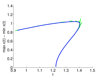
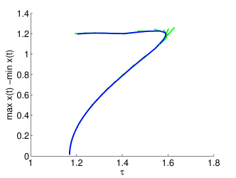
Figure 5: Amplitudes of the periodic solutions arising due to the Hopf Bifurcation as a function of the bifurcation parameter $\tau$ for chimeric (left) and control (right) sets of parameters given in Table 4 for model (3.1). In green the predicted values are marked, while in blue the corrected ones.

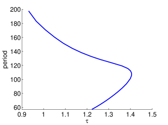
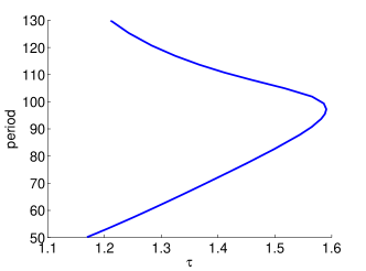
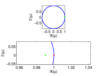
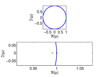
Figure 6: Top: Periods of periodic solutions arising from the Hopf bifurcations as a function of bifurcation parameter $\tau$ for chimeric set of parameters (left) and control set of parameters (right) for model (3.1). Middle and bottom: Floquet multipliers plotted on the complex plain for the periodic solutions near the bifurcation points for chimeric (left) and control (right) sets of parameters for model (3.1). In the bottom row the zoom of the results form the middle row is presented. For all simulations model parameters are given in Table 4.

In Figure 6 (top) the period of periodic solutions arising from the Hopf bifurcations as a function of $\tau$ for control and chimeric sets of parameters are presented. The directly calculated (Theorem 3.3) values of the periods for critical values of bifurcation parameter are $50.1363$ and $57.3715$ for control and chimeric sets of parameters, respectively, see Table 5. Calculating the same for the non-scaled model gives periods of approx. $107$ and $122$ days for the control and chimeric sets of parameters, respectively. These pattern agrees with 3-4 months oscillations observed for the clinical data for certain kinds of human leukemias and also agrees with oscillatory growth of human and rat tumour cell lines reported in [44, 45, 46] or in [47] for non-Hodgkin’s lymphoma.

Interesting is that such recurrent patterns of tumour remission and re-growth have also been clinically observed for immunized BALB/c mice, where mice where initially immunized with BCL₁-Idiotype before the injection of $10^{6}$ BCL₁ tumour cells and without any further immunization, [35]. For such experiment the level of Anti-Id in serum and spleen sizes where followed for a period of 115 days showing that in several mice the spontanous regression followed by splenomegaly was observed, compare Figure 5 in [35]. Moreover, Figure 6 (top) indicates that the periods of the periodic solutions increase with the increase of the bifurcation parameter thus, for larger time lags in the reaction of the immune system to the presence of antigens, larger periods of oscillation of the tumour mass and immunity are observed.

In Figure 6 (middle and bottom) the Floquet multipliers plotted on the complex plain for both sets of estimated parameters are presented. Clearly, the multiplier $(0,1)$ is the trivial one that always exists for the autonomous systems, while the ones inside the circle has modulus smaller than $1$. Since periodic solutions are stable if all, except (0,1), multipliers have modulus smaller than one, one concludes that for the parameter values given in Table 4 the arising periodic solutions are stable. This implies that the supercritical Hopf bifurcations for both sets of parameters are observed, confirming our previous results presented in Figure 5. From the biological or medical point of view supercritical Hopf bifurcation is considered as a safe bifurcation (of course assuming that the amplitude of periodic solutions can not be too large), since although the steady state becomes unstable for larger values of the bifurcation parameter the new born periodic solutions are stable. In such situations a local stable limit cycle around the dormant tumour steady state occurs and again some kind of boundedness of tumour growth is observed. Such oscillations around the steady state corresponds to situation where the tumour grows and shrinks with no application of additional treatment, see the experimental tumour volume data from [44, 45] or [46].

6 Discussion

In this paper the interaction between tumour and immune system by a system of non-linear differential equations with discrete delay, representing time lag in the reaction of immune system to recognition of the antigens, is described. The mathematical properties of proposed model such as: existence, uniqueness and non-negativity of solutions are studied. The presented study focusses on the on the stability of the steady states depending on the value of the bifurcation parameter, which is the time delay. The direct conditions for the stability of the steady states are derived in this paper. In the general case, it is shown that depending on assumptions on the model parameters the stability of the system changes due to Hopf bifurcation for sufficiently large delay. Moreover, only one such stability switch is possible. Additionally, it is shown that the unstable (for $\tau=0$) steady states remain unstable independently of the values of delay.

Next, the proposed model is calibrated with two sets of the experimental data for BCL₁ tumour cells injected to the mice spleens, [35], with MSEs at the level of 3.57% and 0.14%. For the estimated values of parameters, the proposed model is further validated with other experiments for different initial numbers of injected cells. For both sets of estimated values of the parameters the considered model has two positive steady states and one unstable semi-trivial steady state. For the chimeric set of parameters there are stable and unstable positive steady states, which indicate a local stabilization (dormancy) of tumour growth at finite size if the initial size of tumour is sufficiently small (as in case of considered experimental setup) or infinite tumour growth otherwise. For the estimated control set of parameters both positive steady states are unstable, however the periodic orbits exist. That means that depending on the initial conditions the unrestricted tumour growth (as for the control set of parameters) or periodic oscillations of tumour size are observed.

The second coordinates of the positive stable steady state for the chimeric set of the parameters and positive steady state (that is stable for sufficiently small delay) for the control set of parameters are similar. Hence, by decreasing the time response of the immune system to the presence of the tumour cells one might stabilize the uncontrolled tumour growth in case of the control experiment.

Additionally, for both estimated sets of parameters (except time delay treated as a bifurcation parameter) the presented analytical study is extended by investigating the stability of the new born periodic orbits and thus the type of existing Hopf bifurcations. It should be pointed out that the oscillatory behaviour of the multicellular tumour volume was experimentally observed, even without administration of any treatment, as reported for the in vitro experiments for human and rat cell lines reported in [45] and [44]. Such oscillations are explained e.g. as the effect of non-linear feedback between proliferation at the multicellular tumours surface and invasion of the surrounding by tumour cells leaving the spheroid surface however other scenarios are also discussed. The oscillating growth phenomenon is also observed for the in vivo studies and take place for e.g. the mice initially immunized with BCL₁-Idiotype before the injection of $10^{6}$ BCL₁ tumour cells or in non-Hodgkin’s lymphoma [47].

Although the model is rather simple, its dynamics might be complex and reflect a number of bio-medical phenomena such as: therapy failure considered as a modification of model parameters, i.e. an unrestricted growth of the tumour; stabilisation (at least temporary) of tumour growth at a finite size – dormancy; and desirable regression of the tumour. If the initial size of the tumour (or rather amount of antigens) is strictly greater than zero, then according to the values of the model parameters seven different scenarios are possible: (i) asymptotic unrestricted growth of the tumour independently of the initial tumour size; (ii) stabilisation of the tumour growth independently of initial tumour size (existence of globally stable equilibrium); (iii) global eradication of the tumour by the immune system independently of the initial tumour size; (iv) local stabilisation of tumour growth at a certain finite size (if the initial tumour size is sufficiently small one observes stabilisation of the tumour growth at a finite size, otherwise unrestricted growth); (v) local eradication of the tumour by the immune system (for sufficiently small initial size tumour will be eradicated by the immune system, otherwise it will grow unrestrictedly); (vi) bi-stability with eradication for sufficiently small initial tumour, stabilisation on a finite size of tumour of medium initial size and unrestricted growth for large initial tumour when two locally stable steady states co-exist; and finally (vii) recurrent patterns of tumour remission and re-growth. The first six of these features can be observed for the model without time delay, while the last one it is not possible since the ODE model has no periodic solutions. Hence, the DDE model can reflect the oscillatory phenomenon observed for a range of tumour types and in particular in lymphoma.

The main goal of the any-anticancer therapies is to treat disease or at least control its progression. Form the mathematical point of view this means that one wishes to ensure that the trajectories of the system are in the region of attraction of the proper steady states. To do that at the level of the considered model one can try to increase or decrease some of the parameters. In the context of immunotherapy several attempts to increase the immune system efficiency or the creation of anti-tumour immunity were already proposed in many different ways [1, 48, 49]. One can consider the increase of the native immunity e.g. by proper incubation of a patient’s natural killer lymphocytes to enhance their activity and later by their infusion of them into the patient body. In the mathematical language that would mean the increase of the $\omega$ parameter which is crucial for reaching the global or local eradication of the tumour or the bi-stability phenomenon (depending on the values of the other system parameters). Recall that $\omega=wc/(ur)$. Clearly, since the natural lymphocyte death rate ($u$) and the tumour growth rate ($r$) are rather out of reach of immunotherapy one should thus focus on increasing $w$ and $c$ parameters, that is stimulation of the production strength and the effectiveness of effector cells. The increase of the effective cells can be reached by the infusions of the cells grown ex vivo, while the increase of the killing effectiveness of the cells can be obtained as the result of the infusion of properly chosen cytokines, [1]. On the other hand, parameter $r$ can be for example decreased by different types of chemotherapies. Another parameter that has an essential role in determining the range of the controlled tumour growth is the stimulation strength $\rho=a/u$. If the tumour antigens are not presented to the lymphocytes, one can increase $a$ by method of artificial loading of the of antigen-presenting calls with tumour antigen. The effectiveness of such an approach will be dictated by the values of the background immunity and strength of the anti-immune activity. In this paper, it is shown that for the model with discrete delay and estimated parameters an increase of the background immunity ($\omega$), as well as the stimulation strength ($\rho$) of the tumour cells on the immune system, causes the increase of the critical delay value for which the Hopf bifurcation is observed, enlarging the stability region for the positive dormant steady state, see Figure 4. Hence, by increasing the background immunity (range is reachable) one might stabilize the unrestricted tumour growth observed for the control experiment.

On the other hand, if one wishes to model the effectiveness of a given therapy or try to increase a given therapeutic effect one should rather directly include these elements in the system, e.g. by adding new terms and considering the optimization problem. That of course would force the additional calibration of the extended model with additional sets of experimental data required. Researchers who are interested in collaborating with experimentalists or clinicians who have access to patients or in vivo animal trial data should feel encouraged to follow this idea. Recently the very promising concept of an anti-tumour vaccines has arisen, [1, 48]. However, due to the discrete nature of the vaccination program, the presented model would need to be adapted to include an impulse-response framework. In that context, the presented calibrated model can be a base for the future study of the effectiveness of a different types of therapies, including the chemotherapy or combined chemo-immunotherapy. One should feel free to modify the proposed model by fitting it to appearing needs. For example one can consider instead of the exponential tumour growth rather the Gompertz one, which takes into account the finite environmental capacity for tumour cells. That might cause an essential qualitative difference between models. However, it is still an open question. On the other hand, to fit even better proposed model with the experimental data one could instead of the discrete delay consider the distributed one that often better reflects the real measurements.

References

- [1] H. Schreiber, Tumor immunology, in: W. E. Paul (Ed.), Fundamental Immunology, Lippincott-Raven, Philadelphia, 1999, pp. 1237–1270.
- [2] B. Alberts, A. Johnson, J. Lewis, M. Raff, K. Roberts, P. Walter, Molecular Biology of the Cell, 5th Edition, Garland Science, 2008.
- [3] D. Prikrylova, M. Jilek, J. Waniewski, Mathematical modelling of the immune response, CRC Press.
-
[4]
V. A. Kuznetsov, I. A. Makalkin, M. A. Taylor, A. S. Perelson,
Nonlinear dynamics of immunogenic
tumors: Parameter estimation and global bifurcation analysis, Bull. Math.
Biol. 56 (2) (1994) 295–321.
doi:10.1007/bf02460644.
URL http://dx.doi.org/10.1007/BF02460644 - [5] N. Kronik, Y. Kogan, V. Vainstein, Z. Agur, Improving alloreactive CTL immunotherapy for malignant gliomas using a simulation model of their interactive dynamics, Cancer Immunol. Immunother. 57 (2008) 425–439.
- [6] Y. Kogan, U. Foryś, Z. Agur, N. Kronik, O. Shukron, Cellular immunotherapy for high grade gliomas: mathematical analysis deriving efficacious infusion rates based on patient requirements, SIAM J. Appl. Math. 70 (6) (2010) 1953–1976.
- [7] N. Kronik, Y. Kogan, M. Elishmereni, K. Halevi-Tobias, S. Vuk-Pavlović, Z. Agur, Predicting outcomes of prostate cancer immunotherapy by personalized mathematical models, PLoS ONE 5 (12) (2010) e15482. doi:10.1371/journal.pone.0015482.
-
[8]
S. Feyissa, S. Banerjee,
Delay-induced
oscillatory dynamics in humoral mediated immune response with two time
delays, Nonlinear Anal. Real World Appl. 14 (1) (2013) 35–52.
doi:10.1016/j.nonrwa.2012.05.001.
URL http://dx.doi.org/10.1016/j.nonrwa.2012.05.001 - [9] U. Foryś, Global analysis of Marchuk’s model in case of strong immune system, J. Biol. Systems 8 (2000) 331–346.
- [10] U. Foryś, Global analysis of Marchuk’s model in a case of weak immune system, Math. Comput. Modelling 25 (1997) 97–106.
- [11] U. Foryś, Stability and bifurcations for the chronic state in Marchuk’s model of an immune system, J. Math. Anal. Appl. 352 (2009) 922–942.
- [12] U. Foryś, Marchuk’s model of immune system dynamics with application to tumour growth, J. Theor. Med. 4 (1) (2002) 85–93.
-
[13]
D. Kirschner, J. C. Panetta,
Modeling immunotherapy of the
tumor - immune interaction, J. Math. Biol. 37 (3) (1998) 235–252.
doi:10.1007/s002850050127.
URL http://dx.doi.org/10.1007/s002850050127 -
[14]
O. Sotolongo-Costa, L. Morales Molina, D. Rodriguez Perez, J. Antoranz,
M. Chacon Reyes,
Behavior of tumors
under nonstationary therapy, Phys. D 178 (3-4) (2003) 242–253.
doi:10.1016/s0167-2789(03)00005-8.
URL http://dx.doi.org/10.1016/S0167-2789(03)00005-8 - [15] M. Galach, Dynamics of the tumour-immune system competition: The effect of time delay, Int. J. Appl. Math. Comput. Sci. 13 (2003) 395–406.
-
[16]
A. d’Onofrio, A general
framework for modeling tumor-immune system competition and immunotherapy:
Mathematical analysis and biomedical inferences, Phys. D 208 (3-4) (2005)
220–235.
doi:10.1016/j.physd.2005.06.032.
URL http://dx.doi.org/10.1016/j.physd.2005.06.032 - [17] R. Yafia, Hopf bifurcation in differential equations with delay for tumour–immune system competition model, SIAM J. Appl. Math. 67 (6) (2007) 1693–1703.
-
[18]
D. Rodriguez-Perez, O. Sotolongo-Grau, R. Espinosa Riquelme,
O. Sotolongo-Costa, J. A. Santos Miranda, J. C. Antoranz,
Assessment of cancer
immunotherapy outcome in terms of the immune response time features, Math.
Med. Biol. 24 (3) (2007) 287–300.
doi:10.1093/imammb/dqm003.
URL http://dx.doi.org/10.1093/imammb/dqm003 - [19] U. Foryś, J. Waniewski, P. Zhivkov, Anti-tumor immunity and tumor anti-immunity in a mathematical model of tumor immunotherapy, J. Biol. Sys. 14(1) (2006) 13–30.
- [20] S. Banerjee, R. Sarkar, Delay-induced model for tumor-immune interaction and control of malignant tumor growth, BioSystems 91 (2007) 268–288.
- [21] A. d’Onofrio, F. Gatti, P. Cerrai, L. Freschi, Delay-induced oscillatory dynamics of tumour–immune system interaction, Math. Comput. Modelling 51 (5) (2010) 572–591.
- [22] M. Piotrowska, M. Bodnar, J. Poleszczuk, U. Foryś, Mathematical modelling of immune reaction against gliomas: sensitivity analysis and influence of delays, Nonlinear Anal. Real World Appl. 14 (2013) 1601–1620. doi:10.1016/j.nonrwa.2012.10.020.
-
[23]
F. A. Rihan, M. Safan, M. A. Abdeen, D. Abdel Rahman,
Qualitative and computational
analysis of a mathematical model for tumor-immune interactions, J. Appl.
Math. 2012 (2012) 19.
doi:10.1155/2012/475720.
URL http://dx.doi.org/10.1155/2012/475720 -
[24]
P. Bi, S. Ruan, Bifurcations in
delay differential equations and applications to tumor and immune system
interaction models, SIAM J. Appl. Dyn. Syst. 12 (4) (2013) 1847–1888.
doi:10.1137/120887898.
URL http://dx.doi.org/10.1137/120887898 -
[25]
F. Rihan, D. Abdel Rahman, S. Lakshmanan, A. Alkhajeh,
A time delay model of
tumour-immune system interactions: Global dynamics, parameter estimation,
sensitivity analysis, Appl. Math. Comput. 232 (2014) 606–623.
doi:10.1016/j.amc.2014.01.111.
URL http://dx.doi.org/10.1016/j.amc.2014.01.111 -
[26]
F. Frascoli, P. S. Kim, B. D. Hughes, K. A. Landman,
A dynamical model of
tumour immunotherapy, Math. Biosci. 253 (2014) 50–62.
doi:10.1016/j.mbs.2014.04.003.
URL http://dx.doi.org/10.1016/j.mbs.2014.04.003 - [27] G. Bell, Predator-pray equation simulating an immune response, Math. Biosci. 16 (1973) 291–314.
- [28] H. Mayer, K. Zaenker, U. an der Heiden, A basic mathematical model of the immune response, Chaos 5 (1995) 155–161.
- [29] L. de Pillis, A. Radunskaya, A mathematical tumor model with immune resistance and drug therapy: An optimal control approach, Journal of Theoretical Medicine 3 (2001) 79–100.
- [30] G. E. Hutchinson, Circular casual systems in ecology, Ann. N.Y. Acad. Sci. 50 (1948) 221–246.
- [31] M. Piotrowska, U. Foryś, The nature of Hopf bifurcation for the Gompertz model with delays, Math. Comput. Modelling 54 (2011) 2183–2198. doi:10.1016/j.mcm.2011.05.027.
-
[32]
M. Bodanr, M. Piotrowska, U. Foryś,
Gompertz model with delays
and treatment: Mathematical analysis, Math. Biosci. Eng. 10 (3) (2013)
551–563.
doi:10.3934/mbe.2013.10.551.
URL http://dx.doi.org/10.3934/mbe.2013.10.551 - [33] J. Hale, V. S. Lunel, Introduction to Functional Differential Equations (Applied Mathematical Sciences), 1st Edition, Springer, 1993.
- [34] K. L. Cooke, P. Van Den Driessche, On zeroes of some transcendental equations, Funkcial. Ekvac. 29 (1) (1986) 77–90.
- [35] J. W. Uhr, T. Tucker, R. D. May, H. Siu, E. S. Vitetta, Cancer dormancy: Studies of the murine bcl 1 lymphoma., Cancer Res. (Suppl.) 51 (1991) 5045s–5053s.
-
[36]
K. Roesch, D. Hasenclever, M. Scholz,
Modelling lymphoma therapy
and outcome, Bulletin of Mathematical Biology 76 (2) (2013) 401–430.
doi:10.1007/s11538-013-9925-3.
URL http://dx.doi.org/10.1007/s11538-013-9925-3 - [37] M. Tubiana, Tumor cell proliferation kinetics and tumour growth rate., Rev. Oncol. 2 (1989) 113–121.
- [38] R. H. W. S. R. Reynolds, C. W., R. B. Herberman, Measurements of the in vivo turnover rates of rat peripheral blood and spleen large granular lymphocytes., Natural Irnmun. Cell Growth Regul 9 (1985) 272.
-
[39]
J. Kennedy, R. Eberhart,
Particle swarm
optimization, Proceedings of ICNNIV95 - International Conference on Neural
Networksdoi:10.1109/icnn.1995.488968.
URL http://dx.doi.org/10.1109/ICNN.1995.488968 - [40] Y. Shi, R. Eberhart, A modified particle swarm optimizer, Proceedings of IEEE International Conference on Evolutionary Computation (1998) 69–73.
-
[41]
M. Clerc, J. Kennedy, The particle
swarm - explosion, stability, and convergence in a multidimensional complex
space, IEEE Trans. Evol. Computat. 6 (1) (2002) 58–73.
doi:10.1109/4235.985692.
URL http://dx.doi.org/10.1109/4235.985692 - [42] G. S. K. Engelborghs, T. Lyzyanina, Dde-biftool v. 2.00: a matlab package for bifurcation analysis of delay differential equations, Ph.D. thesis, Department of Computer Science, K.U.Leuven, Leuven, Belgium (2001).
- [43] K. Engelborghs, T. Luzyanina, D. Roose, Numerical bifurcation analysis of delay differential equations using dde-biftool, ACM Trans. Math. Softw. 28 (1) (2002) 1–21. doi:10.1145/513001.513002.
-
[44]
R. Chignola, A. Schenetti, E. Chiesa, R. Foroni, S. Sartpris, A. Brendolan,
G. Tridente, G. Andrighetto, D. Liberati,
Oscillating
growth patterns of multicellular tumour spheroids, Cell Prolif. 32 (1)
(1999) 39–48.
doi:10.1046/j.1365-2184.1999.3210039.x.
URL http://dx.doi.org/10.1046/j.1365-2184.1999.3210039.x -
[45]
R. Chignola, A. Schenetti, G. Andrighetto, E. Chiesa, R. Foroni, S. Sartoris,
G. Tridente, D. Liberati,
Forecasting the
growth of multicell tumour spheroids: implications for the dynamic growth of
solid tumours, Cell Prolif 33 (4) (2000) 219–229.
doi:10.1046/j.1365-2184.2000.00174.x.
URL http://dx.doi.org/10.1046/j.1365-2184.2000.00174.x -
[46]
A. S. Gliozzi, C. Guiot, R. Chignola, P. P. Delsanto,
Oscillations in
growth of multicellular tumour spheroids: a revisited quantitative analysis,
Cell Prolif. 43 (4) (2010) 344–353.
doi:10.1111/j.1365-2184.2010.00683.x.
URL http://dx.doi.org/10.1111/j.1365-2184.2010.00683.x - [47] J. G. Krikorian, G. S. Portlock, D. P. Cooney, S. A. Rosenberg, Spontaneous regression of non-hodgkin’s lymphoma: a report of nine cases., Cancer (Phila.) 46 (1980) 2093–2099.
- [48] J. Timmerman, R. Levy, Dentritic cell vaccines for cancer immunotherapy, Ann. Rev. Med. 50 (1999) 507–529.
- [49] P.-L. Lollini, G. Forni, Antitumor vaccines: is it possible to prevent a tumor?, Cancer Immunol. Immunother. 51 (2002) 409–416.