Tests for separability in nonparametric covariance operators of random surfaces

Abstract

. The assumption of separability of the covariance operator for a random image or hypersurface can be of substantial use in applications, especially in situations where the accurate estimation of the full covariance structure is unfeasible, either for computational reasons, or due to a small sample size. However, inferential tools to verify this assumption are somewhat lacking in high-dimensional or functional data analysis settings, where this assumption is most relevant. We propose here to test separability by focusing on $K$-dimensional projections of the difference between the covariance operator and a nonparametric separable approximation. The subspace we project onto is one generated by the eigenfunctions of the covariance operator estimated under the separability hypothesis, negating the need to ever estimate the full non-separable covariance. We show that the rescaled difference of the sample covariance operator with its separable approximation is asymptotically Gaussian. As a by-product of this result, we derive asymptotically pivotal tests under Gaussian assumptions, and propose bootstrap methods for approximating the distribution of the test statistics. We probe the finite sample performance through simulations studies, and present an application to log-spectrogram images from a phonetic linguistics dataset.

Keywords:

Acoustic Phonetic Data, Bootstrap, Dimensional Reduction, Functional Data, Partial Trace, Sparsity.

1 Introduction

Many applications involve hypersurface data, data that is both functional (as in functional data analysis, see e.g. Ramsay & Silverman, 2005; Ferraty & Vieu, 2006; Horváth & Kokoszka, 2012a; Wang et al., 2015) and multidimensional. Examples abound and include images from medical devices such as MRI (Lindquist, 2008) or PET (Worsley et al., 1996), spectrograms derived from audio signals (Rabiner & Schafer, 1978, and as in the application we consider in Section 4) or geolocalized data (see, e.g., Secchi et al., 2015). In these kinds of problem, the number of available observations (hypersurfaces) is often small relative to the high-dimensional nature of the individual observation, and not usually large enough to estimate a full multivariate covariance function.

It is usually, therefore, necessary to make some simplifying assumptions about the data or their covariance structure. If the covariance structure is of interest, such as for PCA or network modeling, for instance, it is usually assumed to have some kind of lower dimensional structure. Traditionally, this translates into a sparsity assumption: one assumes that most entries of the covariance matrix or function are zero. Though being relevant for a number of applications (Tibshirani, 2014), this traditional definition of sparsity may not be appropriate in some cases, such as in imaging, as this can give rise to artefacts in the analysis (for example, holes in an image). In such problems, where the data is multidimensional, a natural assumption that can be made is that the covariance is separable. This assumption greatly simplifies both the estimation and the computational cost in dealing with multivariate covariance functions, while still allowing for a positive definite covariance to be specified. In the context of space-time data $X(s,t)$, for instance, where $s\in[-S,S]^{d}$, $S>0$, denotes the location in space, and $t\in[0,T]$, $T>0$, is the time index, the assumption of separability translates into

$$c(s,t,s^{\prime},t^{\prime})=c_{1}(s,s^{\prime})c_{2}(t,t^{\prime}),\quad s,s^{\prime}\in[-S,S]^{d};t,t^{\prime}\in[0,T],$$ (1.1)

where $c$, $c_{1}$, and $c_{2}$, are respectively the full covariance function, the space covariance function and the time covariance function. In words, this means that the full covariance function factorises as a product of the spatial covariance function with the time covariance function.

The separability assumption (see e.g. Gneiting et al., 2007; Genton, 2007) simplifies the covariance structure of the process and makes it far easier to estimate; in some sense, the separability assumption results in a estimator of the covariance which has less variance, at the expense of a possible bias. As an illustrative example, consider that we observe a discretized version of the process through measurements on a two dimensional grid (without loss of generality, as the same arguments apply for any dimension greater than $2$) being a $q\times p$ matrix (of course, the functional data analysis approach taken here does not assume that the replications of the process are observed on same grid, nor that they are observed on a grid). Since we are not assuming a parametric form for the covariance, the degrees of freedom in the full covariance are $qp(qp+1)/2$, while the separability assumption reduces them to $q(q+1)/2+p(p+1)/2$. This reflects a dramatic reduction in the dimension of the problem even for moderate value of $q,p$, and overcomes both computational and estimation problems due to the relatively small sample sizes available in applications. For example, for $q=p=10$, we have $qp(qp+1)/2=5050$ degrees of freedom, however, if the separability holds, then we have only $q(q+1)+p(p+1)=110$ degrees of freedom. Of course, this is only one example, and our approach is not restricted to data on a grid, but this illustrates the computational savings that such assumptions can possess.

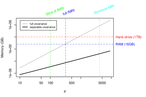
Figure 1: Memory required to store the full covariance and the separable covariance of $p\times p$ matrix data, as a function of $p$. Several types of data related to Neuroimaging (structural and functional Magnetic Resonance Imaging) are used as exemplars of data sizes, as they naturally have multidimensional structure.

Three related computational classes of problem can be identified. In the first case, the full covariance structure can be computed and stored. In the second one, it is still possible, although burdensome, to compute the full covariance matrix but it can not be stored, while the last class includes problems where even computation of the full covariance is infeasible. The values of $q,p$ that set the boundaries for these classes depend of course on the available hardware and they are rapidly changing. At the present time however, for widely available systems, storage is feasible up to $q,p\approx 100$ while computation becomes unfeasible when $q,p$ get close to $1000$ (see Figure 1). On the contrary, a separable covariance structure can be usually both computed and stored without effort even for these sizes of problem. We would like to stress however that the constraints coming from the need for statistical accuracy are usually tighter. The estimation of the full covariance structure even for $q,p=100$ presents about $5\times 10^{7}$ unknown parameters, when typical sample sizes are in the order of hundreds at most. If we are able to assume separability, we can rely on far more accurate estimates.

While the separability assumption can be very useful, and is indeed often implicitly made in many higher dimensional applications when using isotropic smoothing (Worsley et al., 1996; Lindquist, 2008), very little has been done to develop tools to assess its validity on a case by case basis. In the classical multivariate setup, some tests for the separability assumption are available. These have been mainly developed in the field of spatial statistics (see Lu & Zimmerman, 2005; Fuentes, 2006, and references therein), where the discussion of separable covariance functions is well-established, or for applications involving repeated measures (Mitchell et al., 2005). These methods, however, rely on the estimation of the full multidimensional covariance structure, which can be troublesome. It is sometimes possible to circumvent this problem by considering a parametric model for the full covariance structure (Simpson, 2010; Simpson et al., 2014; Liu et al., 2014). On the contrary, when the covariance is being non-parametrically specified, as will be the case in this paper, estimation of the full covariance is at best computationally complex with large estimation errors, and in many cases simply computationally infeasible. Indeed, we highlight that, while the focus of this paper is on checking the viability of a separable structure for the covariance, this is done without any parametric assumption on the form of $c_{1}(s,s^{\prime})$ and $c_{2}(t,t^{\prime})$, thus allowing for the maximum flexibility. This is opposed to assuming a parametric separable form with only few unknown parameters, which is usually too restrictive in many applications, something that has led to separability being rightly criticised and viewed with suspicion in the spatio-temporal statistics literature (Gneiting, 2002; Gneiting et al., 2007). Moreover, the methods we develop here are aimed to applications typical of functional data, where replicates from the underlying random process are available. This is different from the spatio-temporal setting, where usually only one realization of the process is observed. See also Constantinou et al. (2015) for another approach to test for separability in functional data.

It is important to notice that a separable covariance structure (or equivalently, a separable correlation structure) is not necessarily connected with the original data being separable. Furthermore, sums or differences of separable hypersurfaces are not necessarily separable. On the other hand, the error structure may be separable even if the mean is not. Given that in many applications of functional data analysis, the estimation of the covariance is the first step in the analysis, we concentrate on covariance separability. Indeed, covariance separability is an extremely useful assumption as it implies separability of the eigenfunctions, allowing computationally efficient estimation of the eigenfunctions (and principal components). Even if separability is misspecified, separable eigenfunctions can still form a basis representation for the data, they simply no longer carry optimal efficiency guarantees in this case (Aston & Kirch, 2012), but can often have near-optimality under the appropriate assumptions (Chen et al., 2015) .

In this paper, we propose a test to verify if the data at hand are in agreement with a separability assumption. Our test does not require the estimation of the full covariance structure, but only the estimation of the separable structure (1.1), thus avoiding both the computational issues and the diminished accuracy involved in the former. To do this, we rely on a strategy from Functional Data Analysis (Ramsay & Silverman, 2002, 2005; Ferraty & Vieu, 2006; Ramsay et al., 2009; Horváth & Kokoszka, 2012b), which consists in projecting the observations onto a carefully chosen low-dimensional subspace. The key fact for the success of our approach is that, under the null hypothesis, it is possible to determine this subspace using only the marginal covariance functions. While the optimal choice for the dimension of this subspace is a non-trivial problem, some insight can be obtained through our extensive simulation studies (Section 4.1). Ultimately, the proposed test checks the separability in the chosen subspace, which will often be the focus of following analyses.

The paper proceeds as follows. In Section 2, we examine the ideas behind separability, propose a separable approximation of a covariance operator, and study the asymptotics of the difference between the sample covariance operator and its separable approximation. This difference will be the building block of the testing procedures introduced in Section 3, and whose distribution we propose to approximate by bootstrap techniques. In Section 4, we investigate by means of simulation studies the finite sample behaviour of our testing procedures and apply our methods to acoustic phonetic data. A conclusion, given in Section 5, summarizes the main contributions of this paper. Proofs are collected in appendices A, B, and C, while implementation details, theoretical background and additional figures can be found in the appendices E, D and F. All the tests introduced in the paper are available as an R package covsep (Tavakoli, 2016), available on the Comprehensive R Archive Network (CRAN).

For notational simplicity, the proposed method will be described for two dimensional functional data (e.g. random surfaces), hence a four dimensional covariance structure (i.e. the covariance of a random surface), but the generalization to higher dimensional cases is straightforward. The methodology is developed in general for data that take values in a Hilbert space, but the case of square integrable surfaces—being relevant for the case of acoustic phonetic data—is used throughout the paper as a demonstration. We recall that the proposed approach is not restricted to data observed on a regular grid, although for simplicity of exposition we consider here the case where data are observed densely and a pre-processing smoothing step allows to consider the smooth surfaces as our observations, as happens for example the case of the acoustic phonetic data described in Section 4. If data are observed sparsely, the proposed approach can still be applied but there may be the need to use more appropriate estimators for the marginal covariance functions (see, e.g. Yao et al., n.d.) and these need to satisfy the properties described in Section 2.

2 Separable Covariances: definitions, estimators and asymptotic results

While the general idea of the factorization of a multi-dimensional covariance structure as the product of lower dimensional covariances is easy to describe, the development of a testing procedure asks for a rigorous mathematical definition and the introduction of some technical results. In this section we propose a definition of separability for covariance operators, show how it is possible to estimate a separable version of a covariance operator and evaluate the difference between the empirical covariance operator and its separable version. Moreover, we derive some asymptotic results for these estimators. To do this, we first set the problem in the framework of random elements in Hilbert spaces and their covariance operators. The benefit in doing this is twofold. First, our results become applicable in more general settings (e.g. multidimensional functional data, data on multidimensional grids, fixed size rectangular random matrices) and do not depend on a specific choice of smoothness of the data (which is implicitly assumed when modeling the data as e.g. square integrable surfaces). They only rely on the Hilbert space structure of the space in which the data lie. Second, it highlights the importance of the partial trace operator in the estimation of the separable covariance structure, and how the properties of the partial trace (Appendix C) play a crucial role in the asymptotic behavior of the proposed test statistics. However, to ease explanation, we use the case of the Hilbert space of square integrable surfaces (which shall be used in our linguistic application, see Section 4) as an illustration of our testing procedure.

2.1 Notation

Let us first introduce some definitions and notation about operators in a Hilbert space (see e.g. Gohberg et al., 1990; Kadison & Ringrose, 1997a; Ringrose, 1971). Let $H$ be a real separable Hilbert space (that is, a Hilbert space with a countable orthonormal basis), whose inner product and norm are denoted by $\left\langle\cdot,\cdot\right\rangle$ and ${\left\lVert\cdot\right\rVert}$, respectively. The space of bounded (linear) operators on $H$ is denoted by $\mathcal{S}_{\infty}(H)$, and its norm is ${\left|\kern-0.86108pt\left|\kern-0.86108pt\left|T\right|\kern-0.86108pt\right|\kern-0.86108pt\right|}_{\infty}=\sup_{x\neq 0}{\left\lVert Tx\right\rVert}/{\left\lVert x\right\rVert}$. The space of Hilbert–Schmidt operators on $H$ is denoted by $\mathcal{S}_{2}(H)$, and is a Hilbert space with the inner-product $\left\langle S,T\right\rangle_{\!\!\mathcal{S}_{2}}=\sum_{i\geq 1}\left\langle Se_{i},Te_{i}\right\rangle$ and induced norm ${\left|\kern-0.86108pt\left|\kern-0.86108pt\left|\cdot\right|\kern-0.86108pt\right|\kern-0.86108pt\right|}_{2}$, where $(e_{i})_{i\geq 1}\subset H$ is an orthonormal basis of $H$. The space of trace-class operator on $H$ is denoted by $\mathcal{S}_{1}(H)$, and consists of all compact operators $T$ with finite trace-norm, i.e. ${\left|\kern-0.86108pt\left|\kern-0.86108pt\left|T\right|\kern-0.86108pt\right|\kern-0.86108pt\right|}_{1}=\sum_{n\geq 1}s_{n}(T)<\infty$, where $s_{n}(T)\geq 0$ denotes the $n$-th singular value of $T$. For any trace-class operator $T\in\mathcal{S}_{1}(H)$, we define its trace by $\operatorname{{\mathrm{Tr}}}(T)=\sum_{i\geq 1}\left\langle Te_{i},e_{i}\right\rangle$, where $(e_{i})_{i\geq 1}\subset H$ is an orthonormal basis, and the sum is independent of the choice of the orthonormal basis.

If $H_{1},H_{2}$ are real separable Hilbert spaces, we denote by $H=H_{1}\operatorname*{\otimes}H_{2}$ their tensor product Hilbert space, which is obtained by the completion of all finite sums $\sum_{i,j=1}^{N}u_{i}\operatorname*{\otimes}v_{j}$, $u_{i}\in H_{1},v_{j}\in H_{2}$, under the inner-product $\left\langle u\operatorname*{\otimes}v,z\operatorname*{\otimes}w\right\rangle=\left\langle u,z\right\rangle\left\langle v,w\right\rangle,u,z\in H_{1},z,w\in H_{2}$ (see e.g. Kadison & Ringrose, 1997a). If $C_{1}\in\mathcal{S}_{\infty}(H_{1})$, $C_{2}\in\mathcal{S}_{\infty}(H_{2})$, we denote by $C_{1}\operatorname*{\>\widetilde{\otimes}\>}C_{2}$ the unique linear operator on $H_{1}\operatorname*{\otimes}H_{2}$ satisfying

$$\left(C_{1}\operatorname*{\>\widetilde{\otimes}\>}C_{2}\right)(u\operatorname*{\otimes}v)=C_{1}u\operatorname*{\otimes}C_{2}v,\quad\text{for all }u\in H_{1},v\in H_{2}.$$ (2.1)

It is a bounded operator on $H$, with ${\left|\kern-0.86108pt\left|\kern-0.86108pt\left|C_{1}\operatorname*{\>\widetilde{\otimes}\>}C_{2}\right|\kern-0.86108pt\right|\kern-0.86108pt\right|}_{\infty}={\left|\kern-0.86108pt\left|\kern-0.86108pt\left|C_{1}\right|\kern-0.86108pt\right|\kern-0.86108pt\right|}_{\infty}{\left|\kern-0.86108pt\left|\kern-0.86108pt\left|C_{2}\right|\kern-0.86108pt\right|\kern-0.86108pt\right|}_{\infty}$. Furthermore, if $C_{1}\in\mathcal{S}_{1}(H_{1})$ and $C_{2}\in\mathcal{S}_{1}(H_{2})$, then $C_{1}\operatorname*{\>\widetilde{\otimes}\>}C_{2}\in\mathcal{S}_{1}(H_{1}\operatorname*{\otimes}H_{2})$ and ${\left|\kern-0.86108pt\left|\kern-0.86108pt\left|C_{1}\operatorname*{\>\widetilde{\otimes}\>}C_{2}\right|\kern-0.86108pt\right|\kern-0.86108pt\right|}_{1}={\left|\kern-0.86108pt\left|\kern-0.86108pt\left|C_{1}\right|\kern-0.86108pt\right|\kern-0.86108pt\right|}_{1}{\left|\kern-0.86108pt\left|\kern-0.86108pt\left|C_{2}\right|\kern-0.86108pt\right|\kern-0.86108pt\right|}_{1}$. We denote by $\operatorname{{\mathrm{Tr}}}_{1}:\mathcal{S}_{1}(H_{1}\operatorname*{\otimes}H_{2})\rightarrow\mathcal{S}_{1}(H_{2})$ the partial trace with respect to $H_{1}$. It is the unique bounded linear operator satisfying $\operatorname{{\mathrm{Tr}}}_{1}(A\operatorname*{\>\widetilde{\otimes}\>}B)=\operatorname{{\mathrm{Tr}}}(A)B$, for all $A\in\mathcal{S}_{1}(H_{1}),B\in\mathcal{S}_{1}(H_{2})$. $\operatorname{{\mathrm{Tr}}}_{2}:\mathcal{S}_{1}(H_{1}\operatorname*{\otimes}H_{2})\rightarrow\mathcal{S}_{1}(H_{1})$ is defined symmetrically (see Appendix C for more details).

If $X\in H$ is a random element with $\operatorname{\>{\mathbb{E}}}{\left\lVert X\right\rVert}<\infty$, then $\mu=\operatorname{\>{\mathbb{E}}}X\in H$, the mean of $X$, is well defined. Furthermore, if $\operatorname{\>{\mathbb{E}}}{\left\lVert X\right\rVert}^{2}<\infty$, then $C=\,\>{\mathbb{E}\left[(X-\mu)\operatorname*{\otimes_{2}}(X-\mu)\right]}$ defines the covariance operator of $X$, where $f\operatorname*{\otimes_{2}}g$ is the operator on $H$ defined by $(f\operatorname*{\otimes_{2}}g)h=\left\langle h,g\right\rangle f$, for $f,g,h\in H$. The covariance operator $C$ is a trace-class hermitian operator on $H$, and encodes all the second-order fluctuations of $X$ around its mean.

Using this nomenclature, we are going to deal with random variables belonging to a tensor product Hilbert space. This framework encompasses the situation where $X$ is a random surface, for example a space-time indexed data, i.e. $X=X(s,t),s\in[-S,S]^{d},t\in[0,T]$, $S,T>0$, by setting $H={L^{2}\left([-S,S]^{d}\times[0,T],\mathbb{R}\right)}$, for instance (notice however that additional smoothness assumptions on $X$ would lead to assume that $X$ belongs to some other Hilbert space). In this case, the covariance operator of the random element $X\in{L^{2}\left([-S,S]^{d}\times[0,T],\mathbb{R}\right)}$ satisfies

$$Cf(s,t)=\int_{[-S,S]^{d}}\int_{0}^{T}c(s,t,s^{\prime},t^{\prime})f(s^{\prime},t^{\prime})ds^{\prime}dt^{\prime},\quad s\in[-S,S]^{d},t\in[0,T],$$

$f\in{L^{2}\left([-S,S]^{d}\times[0,T],\mathbb{R}\right)}$, where $c(s,t,s^{\prime},t^{\prime})={{\operatorname{{\mathrm{cov}}}}\left[X(s,t),X(s^{\prime},t^{\prime})\right]}$ is the covariance function of $X$. The space of square integrable surfaces,

$${L^{2}\left([-S,S]^{d}\times[0,T],\mathbb{R}\right)},$$

is a tensor product Hilbert space because it can can be identified with

$${L^{2}\left([-S,S]^{d},\mathbb{R}\right)}\operatorname*{\otimes}{L^{2}\left([0,T],\mathbb{R}\right)}.$$

2.2 Separability

We recall now that we want to define separability so that the covariance function can be written as $c(s,t,s^{\prime},t^{\prime})=c_{1}(s,s^{\prime})c_{2}(t,t^{\prime}),$ for some $c_{1}\in{L^{2}\left([-S,S]^{d}\times[-S,S]^{d},\mathbb{R}\right)}$ and $c_{2}\in{L^{2}\left([0,T]\times[0,T],\mathbb{R}\right)}$. This can be extended to the covariance operator of a random elements $X\in H=H_{1}\operatorname*{\otimes}H_{2}$, where $H_{1},H_{2}$ are arbitrary separable real Hilbert spaces. We call its covariance operator $C$ separable if

$$C=C_{1}\operatorname*{\>\widetilde{\otimes}\>}C_{2},$$ (2.2)

where $C_{1}$, respectively $C_{2}$, are trace-class operators on $H_{1}$, respectively on $H_{2}$, and $C_{1}\operatorname*{\>\widetilde{\otimes}\>}C_{2}$ is defined in (2.1). Notice that though the decomposition (2.2) is not unique, since $C_{1}\operatorname*{\>\widetilde{\otimes}\>}C_{2}=(\alpha C_{1})\operatorname*{\>\widetilde{\otimes}\>}(\alpha^{-1}C_{2})$ for any $\alpha\neq 0$, this will not cause any problem at a later stage since we will ultimately be dealing with the product $C_{1}\operatorname*{\>\widetilde{\otimes}\>}C_{2}$, which is identifiable.

In practice, neither $C$ nor $C_{1}\operatorname*{\>\widetilde{\otimes}\>}C_{2}$ are known. If $X_{1},\ldots,X_{N}\stackrel{{\scriptstyle\text{i.i.d.}}}{{\sim}}X$ and (2.2) holds, the sample covariance operator $\widehat{C}_{N}$ is not necessarily separable in finite samples. However, we can estimate a separable approximation of it by

$$\widehat{C}_{1,N}\operatorname*{\>\widetilde{\otimes}\>}\widehat{C}_{2,N},$$ (2.3)

where $\widehat{C}_{1,N}=\operatorname{{\mathrm{Tr}}}_{2}(\widehat{C}_{N})/\sqrt{\operatorname{{\mathrm{Tr}}}(\widehat{C}_{N})}$, $\widehat{C}_{2,N}=\operatorname{{\mathrm{Tr}}}_{1}(\widehat{C}_{N})/\sqrt{\operatorname{{\mathrm{Tr}}}(\widehat{C}_{N})}$. The intuition behind (2.3) is that

$$\operatorname{{\mathrm{Tr}}}(T)T=\operatorname{{\mathrm{Tr}}}_{2}(T)\operatorname*{\>\widetilde{\otimes}\>}\operatorname{{\mathrm{Tr}}}_{1}(T),$$

for all $T\in\mathcal{S}_{1}(H_{1}\operatorname*{\otimes}H_{2})$ of the form $T=A\operatorname*{\>\widetilde{\otimes}\>}B$, $A\in\mathcal{S}_{1}(H_{1}),B\in\mathcal{S}_{1}(H_{2})$, with $\operatorname{{\mathrm{Tr}}}(T)\neq 0$.

Let us consider again what this means when $X$ is a random element of ${L^{2}\left([-S,S]^{d}\times[0,T],\mathbb{R}\right)}$—i.e. the realization of a space-time process—of which we observe $N$ i.i.d. replications $X_{1},\ldots,X_{N}\sim X$. In this case, Proposition C.2 tells us that if the covariance function is continuous, the operators $\widehat{C}_{1,N}$ and $\widehat{C}_{2,N}$ are defined by

$$\widehat{C}_{1,N}f(s) =\int_{[-S,S]^{d}}\widehat{c}_{1,N}(s,s^{\prime})f(s)ds,\quad f\in{L^{2}\left([-S,S]^{d},\mathbb{R}\right)},$$

$$\widehat{C}_{2,N}g(t) =\int_{0}^{T}\widehat{c}_{2,N}(t,t^{\prime})g(t)dt,\quad g\in{L^{2}\left([0,T],\mathbb{R}\right)},$$

where

$$\widehat{c}_{1,N}(s,s^{\prime}) =\frac{\tilde{c}_{1,N}(s,s^{\prime})}{\sqrt{\int_{[-S,S]^{d}}\tilde{c}_{1,N}(s,s)ds}}, \widehat{c}_{2,N}(t,t^{\prime}) =\frac{\tilde{c}_{2,N}(t,t^{\prime})}{\sqrt{\int_{0}^{T}\tilde{c}_{2,N}(t,t)dt}},$$

and

$$\tilde{c}_{1,N}(s,s^{\prime}) =\frac{1}{N}\sum_{i=1}^{N}\int_{0}^{T}\left(X_{i}(s,t)-\overline{X}(s,t)\right)\left(X_{i}(s^{\prime},t)-\overline{X}(s^{\prime},t)\right)dt=\int_{0}^{T}c_{N}(s,t,s^{\prime},t)dt,$$

$$\tilde{c}_{2,N}(t,t^{\prime}) =\frac{1}{N}\sum_{i=1}^{N}\int_{[-S,S]^{d}}\left(X_{i}(s,t)-\overline{X}(s,t)\right)\left(X_{i}(s,t^{\prime})-\overline{X}(s,t^{\prime})\right)ds=\int_{[-S,S]^{d}}c_{N}(s,t,s,t^{\prime})ds,$$

$$\overline{X}(s,t) =\frac{1}{N}\sum_{i=1}^{N}X_{i}(s,t),\widehat{c}_{N}(s,t,s^{\prime},t^{\prime})=\frac{1}{N}\sum_{i=1}^{N}\left(X_{i}(s,t)-\overline{X}(s,t)\right)\left(X_{i}(s^{\prime},t^{\prime})-\overline{X}(s^{\prime},t^{\prime})\right),$$

for all $s,s^{\prime}\in[-S,S]^{d},t,t^{\prime}\in[0,T]$. The assumption of separability here means that the estimated covariance is written as a product of a purely spatial component and a purely temporal component, thus making both modeling and estimation easier in many practical applications.

We stress again that we aim to develop a test statistic that solely relies on the estimation of the separable components $C_{1}$ and $C_{2}$, and does not require the estimation of the full covariance $C$. We can expect that under the null hypothesis $H_{0}:C=C_{1}\operatorname*{\>\widetilde{\otimes}\>}C_{2}$, the difference $D_{N}=\widehat{C}_{N}-\widehat{C}_{1,N}\operatorname*{\>\widetilde{\otimes}\>}\widehat{C}_{2,N}$ between the sample covariance operator and its separable approximation should take small values. We propose therefore to construct our test statistic by projecting $D_{N}$ onto the first eigenfunctions of $C$, since these encode the directions along which $X$ has the most variability. If we denote by $C_{1}=\sum_{i\geq 1}\lambda_{i}u_{i}\operatorname*{\otimes_{2}}u_{i}$ and $C_{2}=\sum_{j\geq 1}\gamma_{j}v_{j}\operatorname*{\otimes_{2}}v_{j}$ the Mercer decompositions of $C_{1}$ and $C_{2}$, we have

$$C=C_{1}\operatorname*{\>\widetilde{\otimes}\>}C_{2}=\sum_{i,j\geq 1}\lambda_{i}\gamma_{j}(u_{i}\operatorname*{\otimes}v_{j})\operatorname*{{\bigotimes}_{2}}(u_{i}\operatorname*{\otimes}v_{j}),$$

where we have used results from Appendix D.1. The eigenfunctions of $C$ are therefore of the form $u_{r}\operatorname*{\otimes}v_{s}$, where $u_{r}\in H_{1}$ is the $r$-th eigenfunction of $C_{1}$ and $v_{s}\in H_{2}$ is the $s$-th eigenfunction of $C_{2}$. We define a test statistic based on the projection

$$T_{N}(r,s)=\sqrt{N}\left\langle D_{N}(\hat{u}_{r}\operatorname*{\otimes}\hat{v}_{s}),\hat{u}_{r}\operatorname*{\otimes}\hat{v}_{s}\right\rangle,\quad r,s\geq 1\text{ fixed},$$ (2.4)

where we have replaced the eigenfunctions of $C_{1}$ and $C_{2}$ by their empirical counterpart, i.e. the Mercer decompositions of $\widehat{C}_{1,N}$, respectively $\widehat{C}_{2,N}$, are given by $\widehat{C}_{1,N}=\sum_{i\geq 1}\hat{\lambda}_{i}\hat{u}_{i}\operatorname*{\otimes}\hat{u}_{i}$, respectively $\widehat{C}_{2,N}=\sum_{j\geq 1}\hat{\gamma}_{j}\hat{v}_{j}\operatorname*{\otimes}\hat{v}_{j}$. Notice that though the eigenfunctions of $\widehat{C}_{1,N}$ and $\widehat{C}_{2,N}$ are defined up to a multiplicative constant $\alpha=\pm 1$, our test statistic is well defined. The key fact for the practical implementation of the method is that $T_{N}(r,s)$ can be computed without the need to estimate (and store in memory) the operator $D_{N}$, since $T_{N}(r,s)=\sqrt{N}\left(\frac{1}{N}\sum_{k=1}^{N}\left\langle X_{k}-\overline{X}_{N},\widehat{v}_{i}\otimes\widehat{u}_{j}\right\rangle^{2}-\hat{\lambda}_{r}\hat{\gamma}_{s}\right).$ In particular, the computation of $T_{N}(r,s)$ does not require an estimation of the full covariance operator $C$, but only the estimation of the marginal covariance operators $C_{1}$ and $C_{2}$, and their eigenstructure.

2.3 Asymptotics

The theoretical justification for using a projection of $D_{N}$ to define a test procedure is that, under the null hypothesis $H_{0}:C=C_{1}\operatorname*{\>\widetilde{\otimes}\>}C_{2}$, we have ${\left|\kern-0.86108pt\left|\kern-0.86108pt\left|D_{N}\right|\kern-0.86108pt\right|\kern-0.86108pt\right|}_{1}\stackrel{{\scriptstyle p}}{{\longrightarrow}}0$ as $N\rightarrow\infty$, i.e. $D_{N}$ convergences in probability to zero with respect to the trace norm. In fact, we will show in Theorem 2.3 that $\sqrt{N}D_{N}$ is asymptotically Gaussian under the following regularity conditions:

Condition 2.1.

$X$ is a random element of the real Hilbert space $H$ satisfying

$$\sum_{j=1}^{\infty}\left(\,\>{\mathbb{E}\left[\left\langle X,e_{j}\right\rangle^{4}\right]}\right)^{1/4}<\infty,$$ (2.5)

for some orthonormal basis $(e_{j})_{j\geq 1}$ of $H$.

The implications of this condition can be better understood in light of the following remark.

remark 2.2 (Mas (2006)).

1. Condition 2.1 implies that $\operatorname{\>{\mathbb{E}}}{{\left\lVert X\right\rVert}^{4}}<\infty$.

2. If $\operatorname{\>{\mathbb{E}}}{{\left\lVert X\right\rVert}^{4}}<\infty$, then $\sqrt{N}(C_{N}-C)$ converges in distribution to a Gaussian random element of $\mathcal{S}_{2}(H)$ for $N\rightarrow\infty$, with respect to the Hilbert–Schmidt topology. Under Condition 2.1, a stronger form of convergence holds: $\sqrt{N}(C_{N}-C)$ converges in distribution to a random element of $\mathcal{S}_{1}(H)$ for $N\rightarrow\infty$, with respect to the trace-norm topology.

3. If $X$ is Gaussian and $(\lambda_{j})_{j\geq 1}$ is the sequence of eigenvalues of its covariance operator, a sufficient condition for (2.5) is $\sum_{j\geq 1}\sqrt{\lambda_{j}}<\infty$.

Condition 2.1 requires fourth order moments rather than the usual second order moments often assumed in functional data, as in this case we are interested in investigating the variation of the second moment, and hence require assumptions on the fourth order structure. Recall that $\widehat{C}_{N}=\frac{1}{N}\sum_{j=1}^{N}(X_{i}-\overline{X})\operatorname*{\otimes_{2}}(X_{i}-\overline{X})$, where $\overline{X}=N^{-1}\sum_{k=1}^{N}X_{k}$. The following result establishes the asymptotic distribution of $D_{N}=\widehat{C}_{N}-\frac{\operatorname{{\mathrm{Tr}}}_{2}(\widehat{C}_{N})\operatorname*{\>\widetilde{\otimes}\>}\operatorname{{\mathrm{Tr}}}_{1}(\widehat{C}_{N})}{\operatorname{{\mathrm{Tr}}}(\widehat{C}_{N})}$:

theorem 2.3.

Let $H_{1},H_{2}$ be separable real Hilbert spaces, $X_{1},\ldots,X_{N}\sim X$ be i.i.d. random elements on $H_{1}\operatorname*{\otimes}H_{2}$ with covariance operator $C$, and $\operatorname{{\mathrm{Tr}}}{C}\neq 0$.

If $X$ satisfies Condition 2.1 (with $H=H_{1}\operatorname*{\otimes}H_{2}$), then, under the null hypothesis

$$H_{0}:C=C_{1}\operatorname*{\>\widetilde{\otimes}\>}C_{2},\qquad C_{1}\in\mathcal{S}_{1}(H_{1}),C_{2}\in\mathcal{S}_{1}(H_{2}),$$

we have

$$\sqrt{N}\left(\widehat{C}_{N}-\frac{\operatorname{{\mathrm{Tr}}}_{2}(\widehat{C}_{N})\operatorname*{\>\widetilde{\otimes}\>}\operatorname{{\mathrm{Tr}}}_{1}(\widehat{C}_{N})}{\operatorname{{\mathrm{Tr}}}(\widehat{C}_{N})}\right)\stackrel{{\scriptstyle d}}{{\longrightarrow}}Z,\quad\text{as }N\rightarrow\infty,$$ (2.6)

where $Z$ is a Gaussian random element of $\mathcal{S}_{1}(H_{1}\operatorname*{\otimes}H_{2})$ with mean zero, whose covariance structure is given in Lemma A.1.

Condition 2.1 is used here because we need $\sqrt{N}(\widehat{C}_{N}-C)$ to converge in distribution in the topology of the space $\mathcal{S}_{1}(H_{1}\operatorname*{\otimes}H_{2})$; it could be replaced by any (weaker) condition ensuring such convergence. The assumption $\operatorname{{\mathrm{Tr}}}{C}\neq 0$ is equivalent to assuming that $X$ is not almost surely constant.

Proof of Theorem 2.3.

First, notice that $C=C_{1}\operatorname*{\>\widetilde{\otimes}\>}C_{2}=\frac{\operatorname{{\mathrm{Tr}}}_{2}(C)\operatorname*{\>\widetilde{\otimes}\>}\operatorname{{\mathrm{Tr}}}_{1}(C)}{\operatorname{{\mathrm{Tr}}}(C)}$ under $H_{0}$. Therefore, using the linearity of the partial trace, we get

$$\sqrt{N}\left(\widehat{C}_{N}-\frac{\operatorname{{\mathrm{Tr}}}_{2}(\widehat{C}_{N})\operatorname*{\>\widetilde{\otimes}\>}\operatorname{{\mathrm{Tr}}}_{1}(\widehat{C}_{N})}{\operatorname{{\mathrm{Tr}}}(\widehat{C}_{N})}\right) =\sqrt{N}(\widehat{C}_{N}-C)$$

$$\quad+\sqrt{N}\left(\frac{\operatorname{{\mathrm{Tr}}}_{2}(C)\operatorname*{\>\widetilde{\otimes}\>}\operatorname{{\mathrm{Tr}}}_{1}(C)}{\operatorname{{\mathrm{Tr}}}(C)}+\frac{\operatorname{{\mathrm{Tr}}}_{2}(\widehat{C}_{N})\operatorname*{\>\widetilde{\otimes}\>}\operatorname{{\mathrm{Tr}}}_{1}(\widehat{C}_{N})}{\operatorname{{\mathrm{Tr}}}(\widehat{C}_{N})}\right)$$

$$=\sqrt{N}(\widehat{C}_{N}-C)+\frac{\operatorname{{\mathrm{Tr}}}\left(\sqrt{N}(\widehat{C}_{N}-C)\right)C}{\operatorname{{\mathrm{Tr}}}(\widehat{C}_{N})}$$

$$\quad-\frac{\operatorname{{\mathrm{Tr}}}_{2}\left(\sqrt{N}(\widehat{C}_{N}-C)\right)\operatorname*{\>\widetilde{\otimes}\>}\operatorname{{\mathrm{Tr}}}_{1}(C)}{\operatorname{{\mathrm{Tr}}}(\widehat{C}_{N})}$$

$$\quad-\frac{\operatorname{{\mathrm{Tr}}}_{2}(\widehat{C}_{N})\operatorname*{\>\widetilde{\otimes}\>}\operatorname{{\mathrm{Tr}}}_{1}\left(\sqrt{N}(\widehat{C}_{N}-C)\right)}{\operatorname{{\mathrm{Tr}}}(\widehat{C}_{N})}.$$

$$=\Psi\left(\sqrt{N}(\widehat{C}_{N}-C),\widehat{C}_{N}\right),$$

where

$$\Psi(T,S)=T+\frac{\operatorname{{\mathrm{Tr}}}(T)C}{\operatorname{{\mathrm{Tr}}}(S)}-\frac{\operatorname{{\mathrm{Tr}}}_{2}(T)\operatorname*{\>\widetilde{\otimes}\>}\operatorname{{\mathrm{Tr}}}_{1}(C)}{\operatorname{{\mathrm{Tr}}}(S)}-\frac{\operatorname{{\mathrm{Tr}}}_{2}(S)\operatorname*{\>\widetilde{\otimes}\>}\operatorname{{\mathrm{Tr}}}_{1}(T)}{\operatorname{{\mathrm{Tr}}}(S)};\quad T,S\in\mathcal{S}_{1}(H_{1}\operatorname*{\otimes}H_{2}).$$

Notice that the function $\Psi:\mathcal{S}_{1}(H_{1}\operatorname*{\otimes}H_{2})\times\mathcal{S}_{1}(H_{1}\operatorname*{\otimes}H_{2})\rightarrow\mathcal{S}_{1}(H_{1}\operatorname*{\otimes}H_{2})$ is continuous at $(T,S)\in\mathcal{S}_{1}(H_{1}\operatorname*{\otimes}H_{2})\times\mathcal{S}_{1}(H_{1}\operatorname*{\otimes}H_{2})$ in each coordinate, with respect to the trace norm, provided $\operatorname{{\mathrm{Tr}}}(S)\neq 0$. Since $\sqrt{N}(\widehat{C}_{N}-C)$ converges in distribution—under Condition 2.1—to a Gaussian random element $Y\in\mathcal{S}_{1}(H_{1}\operatorname*{\otimes}H_{2})$, with respect to the trace norm ${\left|\kern-0.86108pt\left|\kern-0.86108pt\left|\cdot\right|\kern-0.86108pt\right|\kern-0.86108pt\right|}_{1}$ (see Mas, 2006, Proposition 5), $\Psi\left(\sqrt{N}(\widehat{C}_{N}-C),\widehat{C}_{N}\right)$ converges in distribution to

$$\Psi(Y,C)=Y+\frac{\operatorname{{\mathrm{Tr}}}(Y)C}{\operatorname{{\mathrm{Tr}}}(C)}-\frac{\operatorname{{\mathrm{Tr}}}_{2}(Y)\operatorname*{\>\widetilde{\otimes}\>}\operatorname{{\mathrm{Tr}}}_{1}(C)}{\operatorname{{\mathrm{Tr}}}(C)}-\frac{\operatorname{{\mathrm{Tr}}}_{2}(C)\operatorname*{\>\widetilde{\otimes}\>}\operatorname{{\mathrm{Tr}}}_{1}(Y)}{\operatorname{{\mathrm{Tr}}}(C)}$$ (2.7)

by the continuous mapping theorem in metric spaces (Billingsley, 1999). $\Psi(Y,C)$ is Gaussian because each of the summands of (2.7) are Gaussian. Indeed, the first and second summands are obviously Gaussian, and the last two summands are Gaussian by Proposition C.3, and Proposition D.2. ∎

We can now give the asymptotic distribution of $T_{N}(r,s)$, defined in (2.4) as the (scaled) projection of $D_{N}$ in a direction given by the tensor product of the empirical eigenfunctions $\hat{u}_{r}$ and $\hat{v}_{s}$. The proof of the following result is given in Appendix B.

corollary 2.4.

Under the conditions of Theorem 2.3, if $\mathcal{I}\subset\left\{(i,j):i,j\geq 1\right\}$ is a finite set of indices such that $\lambda_{r}\gamma_{s}>0$ for each $(r,s)\in\mathcal{I}$, then

$$\left(T_{N}(r,s)\right)_{(r,s)\in\mathcal{I}}\stackrel{{\scriptstyle d}}{{\longrightarrow}}N(0,\Sigma),\quad\text{as }N\rightarrow\infty.$$

This means that the vector $\left(T_{N}(r,s)\right)_{(r,s)\in\mathcal{I}}$ is asymptotically multivariate Gaussian, with asymptotic variance-covariance matrix $\Sigma=\left(\Sigma_{(r,s),(r^{\prime},s^{\prime})}\right)_{(r,s),(r^{\prime},s^{\prime})\in\mathcal{I}}$ is given by

$$\Sigma_{(r,s),(r^{\prime},s^{\prime})} =\tilde{\beta}_{rsr^{\prime}s^{\prime}}+\frac{\alpha_{rs}\tilde{\beta}_{r^{\prime}s^{\prime}\cdot\cdot}+\alpha_{r^{\prime}s}\tilde{\beta}_{r\cdot\cdot s^{\prime}}+\alpha_{rs^{\prime}}\tilde{\beta}_{r^{\prime}\cdot\cdot s}+\alpha_{r^{\prime}s^{\prime}}\tilde{\beta}_{rs\cdot\cdot}}{\operatorname{{\mathrm{Tr}}}(C)}$$

$$\qquad+\frac{\alpha_{rs}\alpha_{r^{\prime}s^{\prime}}\tilde{\beta}_{\cdot\cdot\cdot\cdot}}{\operatorname{{\mathrm{Tr}}}(C)^{2}}+\frac{\lambda_{r}\lambda_{r^{\prime}}\tilde{\beta}_{\cdot s\cdot s^{\prime}}}{\operatorname{{\mathrm{Tr}}}(C_{1})^{2}}+\frac{\gamma_{s}\gamma_{s^{\prime}}\tilde{\beta}_{r\cdot r^{\prime}\cdot}}{\operatorname{{\mathrm{Tr}}}(C_{2})^{2}}$$

$$\qquad-\frac{\lambda_{r}\tilde{\beta}_{r^{\prime}s^{\prime}\cdot s}+\lambda_{r^{\prime}}\tilde{\beta}_{rs\cdot s^{\prime}}}{\operatorname{{\mathrm{Tr}}}(C_{1})}-\frac{\gamma_{s}\tilde{\beta}_{r^{\prime}s^{\prime}r\cdot}+\gamma_{s^{\prime}}\tilde{\beta}_{rsr^{\prime}\cdot}}{\operatorname{{\mathrm{Tr}}}(C_{2})}$$

$$\qquad-\frac{\alpha_{rs}}{\operatorname{{\mathrm{Tr}}}(C)}\left(\frac{\gamma_{s^{\prime}}\tilde{\beta}_{r^{\prime}\cdot\cdot\cdot}}{\operatorname{{\mathrm{Tr}}}(C_{2})}+\frac{\lambda_{r^{\prime}}\tilde{\beta}_{\cdot s^{\prime}\cdot\cdot}}{\operatorname{{\mathrm{Tr}}}(C_{1})}\right)$$

$$\qquad-\frac{\alpha_{r^{\prime}s^{\prime}}}{\operatorname{{\mathrm{Tr}}}(C)}\left(\frac{\gamma_{s}\tilde{\beta}_{r\cdot\cdot\cdot}}{\operatorname{{\mathrm{Tr}}}(C_{2})}+\frac{\lambda_{r}\tilde{\beta}_{\cdot s\cdot\cdot}}{\operatorname{{\mathrm{Tr}}}(C_{1})}\right)$$

where $\mu=\,\>{\mathbb{E}\left[X\right]}$, $\alpha_{rs}=\lambda_{r}\gamma_{s}$,

$$\tilde{\beta}_{ijkl}=\,\>{\mathbb{E}\left[\left\langle X-\mu,u_{i}\operatorname*{\otimes}v_{j}\right\rangle^{2}\left\langle X-\mu,u_{k}\operatorname*{\otimes}v_{l}\right\rangle^{2}\right]},$$

and ‘$\,\cdot$’ denotes summation over the corresponding index, i.e. $\tilde{\beta}_{r\cdot jk}=\sum_{i\geq 1}\tilde{\beta}_{rijk}$.

We note that the asymptotic variance-covariance of $\left(T_{N}(r,s)\right)_{(r,s)\in\mathcal{I}}$ depends on the second and fourth order moments of $X$, which is not surprising since it is based on estimators of the covariance of $X$. Under the additional assumption that $X$ is Gaussian, the asymptotic variance-covariance of $\left(T_{N}(r,s)\right)_{(r,s)\in\mathcal{I}}$ can be entirely expressed in terms of the covariance operator $C$. The proof of the following result is given in Appendix B.

corollary 2.5.

Assume the conditions of Theorem 2.3 hold, and that $X$ is Gaussian. If $\mathcal{I}\subset\left\{(i,j):i,j\geq 1\right\}$ is a finite set of indices such that $\lambda_{r}\gamma_{s}>0$ for each $(r,s)\in\mathcal{I}$, then

$$\left(T_{N}(r,s)\right)_{(r,s)\in\mathcal{I}}\stackrel{{\scriptstyle d}}{{\longrightarrow}}N(0,\Sigma),\quad\text{as }N\rightarrow\infty.$$

where

$$\Sigma_{(r,s),(r^{\prime},s^{\prime})} =\frac{2\lambda_{r}\lambda_{r^{\prime}}\gamma_{s}\gamma_{s^{\prime}}}{\operatorname{{\mathrm{Tr}}}(C)^{2}}\left(\delta_{rr^{\prime}}\operatorname{{\mathrm{Tr}}}(C_{1})^{2}+{\left|\kern-0.86108pt\left|\kern-0.86108pt\left|C_{1}\right|\kern-0.86108pt\right|\kern-0.86108pt\right|}_{2}^{2}-(\lambda_{r}+\lambda_{r^{\prime}})\operatorname{{\mathrm{Tr}}}(C_{1})\right)$$

$$\qquad\times\left(\delta_{ss^{\prime}}\operatorname{{\mathrm{Tr}}}(C_{2})^{2}+{\left|\kern-0.86108pt\left|\kern-0.86108pt\left|C_{2}\right|\kern-0.86108pt\right|\kern-0.86108pt\right|}_{2}^{2}-(\gamma_{s}+\gamma_{s^{\prime}})\operatorname{{\mathrm{Tr}}}(C_{2})\right),$$

and $\delta_{ij}=1$ if $i=j$, and zero otherwise. In particular, notice that $\Sigma$ itself is separable.

It will be seen in the next section that even in the case where we use a bootstrap test, knowledge of the asymptotic distribution can be very useful to establish a pivotal bootstrap test, which will be seen to have very good performance in simulation.

3 Separability Tests and Bootstrap Approximations

In this section we use the estimation procedures and the theoretical results presented in Section 2 to develop a test for $H_{0}:C=C_{1}\operatorname*{\>\widetilde{\otimes}\>}C_{2}$, against the alternative that $C$ cannot be written as a tensor product.

First, it is straightforward to define a testing procedure when $X$ is Gaussian. Indeed, if we let

$$G_{N}(r,s)=T_{N}^{2}(r,s)=N\left(\frac{1}{N}\sum_{k=1}^{N}\left\langle X_{k}-\overline{X},\widehat{u}_{r}\otimes\widehat{v}_{s}\right\rangle^{2}-\hat{\lambda}_{r}\hat{\gamma}_{s}\right)^{2},$$ (3.1)

and

$$\hat{\sigma}^{2}(r,s)=\left({\operatorname{{\mathrm{Tr}}}(\widehat{C}_{1,N})^{2}\operatorname{{\mathrm{Tr}}}(\widehat{C}_{2,N})^{2}}\right)^{-1}2\hat{\lambda}_{r}^{2}\hat{\gamma}_{s}^{2}\\ \times\left(\operatorname{{\mathrm{Tr}}}(\widehat{C}_{1,N})^{2}+{\left|\kern-0.86108pt\left|\kern-0.86108pt\left|\widehat{C}_{1,N}\right|\kern-0.86108pt\right|\kern-0.86108pt\right|}_{2}^{2}-2\hat{\lambda}_{r}\operatorname{{\mathrm{Tr}}}(\widehat{C}_{1,N})\right)\\ \times\left(\operatorname{{\mathrm{Tr}}}(\widehat{C}_{2,N})^{2}+{\left|\kern-0.86108pt\left|\kern-0.86108pt\left|\widehat{C}_{2,N}\right|\kern-0.86108pt\right|\kern-0.86108pt\right|}_{2}^{2}-2\hat{\gamma}_{s}\operatorname{{\mathrm{Tr}}}(\widehat{C}_{2,N})\right),$$ (3.2)

then $\hat{\sigma}^{-2}(r,s)G_{N}(r,s)$ is asymptotically $\chi^{2}_{1}$ distributed, and $\{G_{N}^{2}(r,s)>\hat{\sigma}^{2}(r,s)\chi^{2}_{1}(1-\alpha)\}$, where $\chi^{2}_{1}(1-\alpha)$ is the $1-\alpha$ quantile of the $\chi^{2}_{1}$ distribution, would be a rejection region of level approximately $\alpha$, for $\alpha\in[0,1]$ and $N$ large.

Apart for the distributional assumption for $X$ to be Gaussian, this approach suffers also the important limitation that it only tests the separability assumption along one eigendirection. It is possible to extend this approach to take into account several eigendirections. For simplicity, let us consider the case $\mathcal{I}=\left\{1,\ldots,p\right\}\times\left\{1,\ldots,q\right\}$. Denote by $\mathbf{T}_{N}(\mathcal{I})$ the $p\times q$ matrix with entries $(\mathbf{T}_{N}(\mathcal{I}))_{ij}=T_{N}(i,j)$, and let

$$\widetilde{G}_{N}(\mathcal{I})=\left|\hat{\Sigma}_{L,\mathcal{I}}^{-1/2}\mathbf{T}_{N}(\mathcal{I})\hat{\Sigma}_{R,\mathcal{I}}^{-\mathsf{T}/2}\right|^{2},$$ (3.3)

where $|A|^{2}$ denotes the sum of squared entries of a matrix $A$, $A^{-1/2}$ denotes the inverse of (any) square root of the matrix $A$, $A^{-\mathsf{T}/2}=(A^{-1/2})^{\mathsf{T}}$, and the matrices $\hat{\Sigma}_{L,\mathcal{I}}$, respectively $\hat{\Sigma}_{R,\mathcal{I}}$, which are estimators of the row, resp. column, asymptotic covariances of $\mathbf{T}_{N}(\mathcal{I})$, are defined in Appendix E. Then $\widetilde{G}_{N}(\mathcal{I})$ is asymptotically $\chi^{2}_{pq}$ distributed. In the simulation studies (Section 4.1), we consider also an approximate version of this Studentized test statistics, $\widetilde{G}_{N}^{a}(\mathcal{I})=\sum_{(r,s)\in\mathcal{I}}T_{N}^{2}(r,s)/\hat{\sigma}^{2}(r,s),$ which are obtained simply by standardizing marginally each entry $T_{N}^{2}(r,s)$, thus ignoring the dependence between the test statistics associated with different directions. In order to assess the advantage of Studentization, we also consider the non-Studentized test statistic

$$G_{N}(\mathcal{I})=\sum_{(r,s)\in\mathcal{I}}T_{N}^{2}(r,s).$$

The computation details for $\widetilde{G}_{N}$, $T_{N}$, $\hat{\sigma}^{2}(r,s)$, $\hat{\Sigma}_{L,\mathcal{I}}$ and $\hat{\Sigma}_{R,\mathcal{I}}$ are described in Appendix E.

remark 3.1.

Notice that the only test whose asymptotic distribution is parameter free is $\widetilde{G}_{N}(\mathcal{I})$, under Gaussian assumptions. It would in principle be possible to construct an analogous test without the Gaussian assumptions (using Corollary 2.4). However, due to the large number of parameters that would need to be estimated in this case, we expect the asymptotics to come into force only for very large sample sizes (this is actually the case under Gaussian assumptions, specially if the set of projections $\mathcal{I}$ is large, as can be seen in Figure 10). For these reasons, we shall investigate bootstrap approximations to the test statistics.

The choice of the number of eigenfunctions $K$ (the number of elements in $\mathcal{I}$) onto which one should project is not trivial. The popular choice of including enough eigenfunctions to explain a fixed percentage of the variability in the dataset may seem inappropriate in this context, because under the alternative hypothesis there is no guarantee that the separable eigenfunctions explain that percentage of variation.

For fixed $K$, notice that the test at least guarantees the separability in the subspace of the respective $K$ eigenfunctions, which is where the following analysis will be often focused. On the other hand, since our test statistic looks at an estimator of the non-separable component

$$D=C-\frac{\operatorname{{\mathrm{Tr}}}_{2}(C)\operatorname*{\>\widetilde{\otimes}\>}\operatorname{{\mathrm{Tr}}}_{1}(C)}{\operatorname{{\mathrm{Tr}}}(C)},$$

restricted to the subspace spanned by the eigenfunctions $u_{r}\operatorname*{\otimes}v_{s}$, the test takes small values (and thus lacks power) when

$$\left\langle D(u_{r}\operatorname*{\otimes}v_{s}),u_{r}\operatorname*{\otimes}v_{s}\right\rangle=\left\langle D,(u_{r}\operatorname*{\otimes_{2}}u_{r})\operatorname*{\>\widetilde{\otimes}\>}(v_{s}\operatorname*{\otimes_{2}}v_{s})\right\rangle_{\!\!\mathcal{S}_{2}}=0,$$

that is when the non-separable component $D$ is orthogonal to

$$(u_{r}\operatorname*{\otimes_{2}}u_{r})\operatorname*{\>\widetilde{\otimes}\>}(v_{s}\operatorname*{\otimes_{2}}v_{s})$$

with respect to the Hilbert–Schmidt inner product. Thus the proposed test statistic $G_{N}(\mathcal{I})$ is powerful when $D$ is not orthogonal to the subspace

$$V_{\mathcal{I}}=\mathrm{span}\{(u_{i}\operatorname*{\otimes_{2}}u_{i})\operatorname*{\>\widetilde{\otimes}\>}(v_{j}\operatorname*{\otimes_{2}}v_{j}),(i,j)\in\mathcal{I}\},$$

and in general the power of the test for finite sample size depends on the properly rescaled norm of the projection of $D$ onto $V_{\mathcal{I}}$.

In practice, it seems reasonable to use the subset of eigenfunctions that it is possible to estimate accurately given the available sample sizes. The accuracy of the estimates for the eigendirections can be in turn evaluated with bootstrap methods, see e.g. Hall & Hosseini-Nasab (2006) for the case of functional data. A good strategy may also be to consider more than one subset of eigenfunctions and then summarize the response obtained from the different tests using a Bonferroni correction.

As an alternative to these test statistics (based on projections of $D_{N}=C_{N}-C_{1,N}\operatorname*{\>\widetilde{\otimes}\>}C_{2,N}$), we consider also a test based on the squared Hilbert–Schmidt norm of $D_{N}$, i.e. ${\left|\kern-0.86108pt\left|\kern-0.86108pt\left|D_{N}\right|\kern-0.86108pt\right|\kern-0.86108pt\right|}_{2}^{2}$, whose null distribution will be approximated by a bootstrap procedure (this test will be referred to as Hilbert–Schmidt test hereafter). Though it seems that such tests would require one to store the full sample covariance of the data (which could be infeasible), we describe in Appendix E a way of circumventing such problem, although the computation of each entry of the full covariance is still needed. Therefore this could be used only for applications in which the dimension of the discretized covariance matrix is not too large.

In the following, we propose also a bootstrap approach to approximate the distribution of the test statistics $\widetilde{G}_{N}(\mathcal{I})$, $\widetilde{G}^{a}_{N}(\mathcal{I})$ and $G_{N}(\mathcal{I})$, with the aim to improve the finite sample properties of the procedure and to relax the distributional assumption on $X$.

3.1 Parametric Bootstrap

If we assume we know the distribution of $X$ up to its mean $\mu$ and its covariance operator $C$, i.e. $X\sim F(\mu;C)$, we can approximate the distribution of $\widetilde{G}_{N}(\mathcal{I})$, $\widetilde{G}^{a}_{N}(\mathcal{I})$, $G_{N}(\mathcal{I})$ and ${\left|\kern-0.86108pt\left|\kern-0.86108pt\left|D_{N}\right|\kern-0.86108pt\right|\kern-0.86108pt\right|}_{2}^{2}$ under the separability hypothesis via a parametric bootstrap procedure. Since $C_{1,N}\operatorname*{\>\widetilde{\otimes}\>}C_{2,N}$, respectively $\overline{X}$, is an estimate of $C$, respectively $\mu$, we simulate $B$ bootstrap samples $X^{b}_{1},\ldots,X^{b}_{N}\stackrel{{\scriptstyle\text{i.i.d.}}}{{\sim}}F\left(\>\overline{X},C_{1,N}\operatorname*{\>\widetilde{\otimes}\>}C_{2,N}\right)$, for $b=1,\ldots,B$. For each sample, we compute $H_{N}^{b}=H_{N}(X_{1}^{b},\ldots,X_{N}^{b})$, where $H_{N}=G_{N}(\mathcal{I})$, $H_{N}=\widetilde{G}_{N}(\mathcal{I})$, $H_{N}=\widetilde{G}^{a}_{N}(\mathcal{I})$ respectively $H_{N}={\left|\kern-0.86108pt\left|\kern-0.86108pt\left|D_{N}\right|\kern-0.86108pt\right|\kern-0.86108pt\right|}_{2}^{2}$, if we wish to use the non-Studentized projection test, the Studentized projection test, the approximated Studentized version or the Hilbert–Schmidt test, respectively. A formal description of the algorithm for obtaining the $p$-value of the test based on the statistic $H_{N}=H_{N}(X_{1},\ldots,X_{N})$ with the parametric bootstrap can be found in Appendix E, along with the details for the computation of $H_{N}$. We highlight that this procedure does not ask for the estimation of the full covariance structure, but only of its separable approximation, with the exception of the Hilbert–Schmidt test (and even in this case, it is possible to avoid the storage of the full covariance).

3.2 Empirical Bootstrap

In many applications it is not possible to assume a distribution for the random element $X$, and a non-parametric approach is therefore needed. In this setting, we can use the empirical bootstrap to estimate the distribution of the test statistic $G_{N}(\mathcal{I}),\widetilde{G}_{N}(\mathcal{I})$ or ${\left|\kern-0.86108pt\left|\kern-0.86108pt\left|D_{N}\right|\kern-0.86108pt\right|\kern-0.86108pt\right|}_{2}^{2}$ under the null hypothesis $H_{0}:C=C_{1}\operatorname*{\>\widetilde{\otimes}\>}C_{2}$. Let $H_{N}$ denote the test statistic whose distribution is of interest. Based on an i.i.d. sample $X_{1},\ldots,X_{N}\sim X$, we wish to approximate the distribution of $H_{N}$ with the distribution of some test statistic $\Delta_{N}^{*}=\Delta_{N}(X_{1}^{*},\ldots,X_{N}^{*})$, where $X_{1}^{*},\ldots,X_{N}^{*}$ is obtained by drawing with replacement from the set $\left\{X_{1},\ldots,X_{N}\right\}$. Though it is tempting to use $\Delta^{*}_{N}=H_{N}(X_{1}^{*},\ldots,X_{N}^{*})$, this is not an appropriate choice. Indeed, let us look at the case $H_{N}=G_{N}(i,j)$. Notice that the true covariance of $X$ is

$$C=\frac{\operatorname{{\mathrm{Tr}}}_{2}(C)\operatorname*{\>\widetilde{\otimes}\>}\operatorname{{\mathrm{Tr}}}_{1}(C)}{\operatorname{{\mathrm{Tr}}}(C)}+D,$$ (3.4)

where $D$ is a possibly non-zero operator, and that

$$H_{N}^{*}=G_{N}(i,j|X_{1}^{*},\ldots,X_{N}^{*})=N\left\langle(C_{N}^{*}-C_{1,N}^{*}\operatorname*{\>\widetilde{\otimes}\>}C_{2,N}^{*})(\hat{u}_{i}\operatorname*{\otimes}\hat{v}_{j}),\hat{u}_{i}\operatorname*{\otimes}\hat{v}_{j}\right\rangle^{2},$$

where $C_{N}^{*}=C_{N}(X_{1}^{*},\ldots,X_{N}^{*}),C_{1,N}^{*}=C_{1,N}(X_{1}^{*},\ldots,X_{N}^{*}),$ and $C_{2,N}^{*}=C_{2,N}(X_{1}^{*},\ldots,X_{N}^{*})$. Since $(C_{N}^{*}-C_{1,N}^{*}\operatorname*{\>\widetilde{\otimes}\>}C_{2,N}^{*})\approx(C_{N}-C_{1,N}\operatorname*{\>\widetilde{\otimes}\>}C_{2,N})\approx D$, the statistic $H_{N}^{*}$ would approximate the distribution of $H_{N}$ under the hypothesis (3.4), which is not what we want. We therefore propose the following choices of $\Delta_{N}^{*}=\Delta_{n}(X_{1}^{*},\ldots,X_{N}^{*};X_{1},\ldots,X_{N})$, depending on the choice of $H_{N}$:

1. $H_{N}=G_{N}(\mathcal{I})$, $\Delta_{N}^{*}=\sum_{(i,j)\in\mathcal{I}}\left(T_{N}^{*}(i,j)-T_{N}(i,j)\right)^{2}$.

2. $H_{N}=\widetilde{G}_{N}(\mathcal{I})$, $\Delta_{N}^{*}=\left|\left(\hat{\Sigma}^{*}_{L,\mathcal{I}}\right)^{-1/2}\left(\mathbf{T}^{*}_{N}(\mathcal{I})-\mathbf{T}_{N}(\mathcal{I})\right)\left(\hat{\Sigma}^{*}_{R,\mathcal{I}}\right)^{-\mathsf{T}/2}\right|^{2},$ where $\hat{\Sigma}^{*}_{L,\mathcal{I}}=\hat{\Sigma}_{L,\mathcal{I}}(X_{1}^{*},\ldots,X_{N}^{*})$, and $\hat{\Sigma}^{*}_{R,\mathcal{I}}=\hat{\Sigma}_{R,\mathcal{I}}(X_{1}^{*},\ldots,X_{N}^{*})$. are the row, resp. column, covariances estimated from the bootstrap sample.

3. $H_{N}=\widetilde{G}^{a}_{N}(\mathcal{I})$, $\Delta_{N}^{*}=\sum_{(i,j)\in\mathcal{I}}\left(T_{N}^{*}(i,j)-T_{N}(i,j)\right)^{2}/\hat{\sigma}_{*}^{2}(i,j),$ where $\hat{\sigma}_{*}^{2}(i,j)=\hat{\sigma}^{2}(i,j|X_{1}^{*},\ldots,X_{N}^{*})$.

4. $H_{N}={\left|\kern-0.86108pt\left|\kern-0.86108pt\left|D_{N}\right|\kern-0.86108pt\right|\kern-0.86108pt\right|}_{2}^{2}$, $\Delta_{N}^{*}={\left|\kern-0.86108pt\left|\kern-0.86108pt\left|D_{N}^{*}-D_{N}\right|\kern-0.86108pt\right|\kern-0.86108pt\right|}_{2}^{2}$, where $D_{N}^{*}=D_{N}(X_{1}^{*},\ldots,X_{N}^{*})$.

The algorithm to approximate the $p$-value of $H_{N}$ by the empirical bootstrap is described in detail. The basic idea consists of generating $B$ bootstrap samples, computing $\Delta_{N}^{*}$ for each bootstrap sample and looking at the proportion of bootstrap samples for which $\Delta_{N}^{*}$ is larger than the test statistic $H_{N}$ computed from the original sample.

4 Empirical demonstrations of the method

4.1 Simulation studies

We investigated the finite sample behavior of our testing procedures through an intensive reproducible simulation study (its running time is equivalent to approximately 401 days on a single CPU computer). We compared the test based on the asymptotic distribution of (3.1), as well as the tests based on $G_{N}(\mathcal{I}),\widetilde{G}_{N}(\mathcal{I}),\widetilde{G}^{a}_{N}(\mathcal{I})$, and ${\left|\kern-0.86108pt\left|\kern-0.86108pt\left|D_{N}\right|\kern-0.86108pt\right|\kern-0.86108pt\right|}_{2}^{2}$, with the $p$-values obtained via the parametric bootstrap or the empirical bootstrap.

We generated discretized functional data $X_{1},\ldots,X_{N}\in\mathbb{R}^{32\times 7}$ under two scenarios. In the first scenario (Gaussian scenario), the data were generated from a multivariate Gaussian distribution $\mathcal{N}(0,\mathbf{C})$. In the second scenario (Non-Gaussian scenario), the data were generated from a multivariate $t$ distribution with $6$ degrees of freedom and non centrality parameter equal to zero. In the Gaussian scenario, we set $\mathbf{C}=\mathbf{C}^{(\gamma)}$, where

$$\mathbf{C}^{(\gamma)}(i_{1},j_{1},i_{2},j_{2})=(1-\gamma)c_{1}(i_{1},i_{2})c_{2}(j_{1},j_{2})\\ +\gamma\frac{1}{(j_{1}-j_{2})^{2}+1}\exp\left\{-\frac{(i_{1}-i_{2})^{2}}{(j_{1}-j_{2})^{2}+1}\right\},$$ (4.1)

$\gamma\in[0,1];i_{1},i_{2}=1,\ldots,32;j_{1},j_{2}=1,\ldots,7$. The covariances $c_{1}$ and $c_{2}$ used in the simulations can be seen in Figure 2. For the Non-Gaussian scenario, we chose a multivariate $t$ distribution with the correlation structure implied by $\mathbf{C}^{(\gamma)}$, $\gamma\in[0,1];i_{1},i_{2}=1,\ldots,32;j_{1},j_{2}=1,\ldots,7$. The parameter $\gamma\in[0,1]$ controls the departure from the separability of the covariance $\mathbf{C}^{(\gamma)}$: $\gamma=0$ yields a separable covariance, whereas $\gamma=1$ yields a complete non-separable covariance structure (Cressie & Huang, 1999). All the simulations have been performed using the R package covsep (Tavakoli, 2016), available on CRAN, which implements the tests presented in the paper.

 

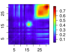
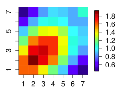
Figure 2: Covariance functions $c_{1}$ (left) and $c_{2}$ (right) used in the simulation study.

For each value of $\gamma\in\{0,0.01,0.02,\ldots,0.1\}$ and $N\in\{10,25,50,100\}$, we performed $1000$ replications for each of the above simulations, and estimated the power of the tests based on the asymptotic distribution of (3.1).

(a) Gaussian scenario

(b) Non Gaussian scenario

Figure 3: Empirical power of the testing procedures in the Gaussian scenario (panel (a)) and non-Gaussian scenario (panel (b)), for $N=10,25,50,100$ and $\mathcal{I}=\mathcal{I}_{1}$. The results shown correspond to the test (3.1) based on its asymptotic distribution ($\cdot\!\cdot\!\cdot\!\cdot\!+\!\cdot\!\cdot\!\cdot\!\cdot$), the Gaussian parametric bootstrap test (solid line with empty circles) and its studentized version (dash-dotted line with empty circles), the empirical parametric bootstrap test (—$\bigtriangleup$—) and its Studentized version (– –$\bigtriangleup$– –), the Gaussian parametric Hilbert–Schmidt test (dash-dotted line with filled circles) and the empirical Hilbert–Schmidt test (dash-dotted line with filled triangles). The horizontal dotted line indicates the nominal level ($5\%$) of the test. Note that the points have been horizontally jittered for better visibility.

We first also estimated the power of the tests $\widetilde{G}_{N}(1,1)$, $G_{N}(1,1)$, and ${\left|\kern-0.86108pt\left|\kern-0.86108pt\left|D_{N}\right|\kern-0.86108pt\right|\kern-0.86108pt\right|}_{2}$, with distributions approximated by a Gaussian parametric bootstrap, and the empirical bootstrap, with $B=1000$. The results are shown in Figure 3. In the Gaussian scenario (Figure 3, panel (a)), the empirical size of all the proposed tests gets closer to the nominal level ($5\%$) as $N$ increases (see also Table 2). Nevertheless, the non-Studentized tests $G_{N}(1,1)$, for both parametric and empirical bootstrap, seem to have a slower convergence with respect to the Studentized version, and even for $N=100$ the level of these tests appear still higher than the nominal one (and a CLT-based 95% confidence interval for the true level does not contain the nominal level in both cases). The empirical bootstrap version of the Hilbert–Schmidt test also fails to respect the nominal level at $N=100$, but its parametric bootstrap counterpart respects the level, even for $N=25$. For $N=25,50,100$, the most powerful tests (amongst those who respect the nominal level) are the parametric and empirical bootstrap versions of $\widetilde{G}_{N}(1,1)$, and they seem to have equal power. The power of the Hilbert–Schmidt test based on the parametric bootstrap seems to be competitive only for $N=100$ and $\gamma=0.1$, and is much lower for other values of the parameters. The test based on the asymptotic distribution does not respect the nominal level for small $N$ but it does when $N$ increases. Indeed, the convergence to the nominal level seems remarkably fast and its power is comparable with those of the parametric and empirical bootstrap tests based on $\widetilde{G}_{N}(1,1)$. Despite being based on an asymptotic result, its performance is quite good also in finite samples, and it is less computationally demanding than the bootstrap tests.

In the non-Gaussian scenario (Figure 3, panel (b)), only the empirical bootstrap version of $\widetilde{G}_{N}(1,1)$ and of the Hilbert–Schmidt test seem to respect the level for $N=10$ (see also Table 2). Amongst these tests, the most powerful one is clearly the empirical bootstrap test based on $\widetilde{G}_{N}(1,1)$. Although the Gaussian parametric bootstrap test has higher empirical power, it does not have the correct level (as expected) and thus cannot be used in a non-Gaussian scenario. Notice also that the test based on the asymptotic distribution of $\widetilde{G}_{N}(1,1)$ (under Gaussian assumptions) does not respects the level of the test even for $N=100$. The same holds for the Gaussian bootstrap version of the Hilbert–Schmidt test. Finally, though the empirical bootstrap version of the Hilbert–Schmidt test respects the level for $N=10,25,50,100$, it has virtually no power for $N=10,25,50$, and has very low power for $N=100$ (at most $0.3$ for $\gamma=0.1$).

As mentioned previously, there is no guarantee that a violation in the separability of $C$ is mostly reflected in the first separable eigensubspace. Therefore, we consider also a larger subspace for the test. Figure 9 shows the empirical power for the asymptotic test, the parametric and empirical bootstrap tests based on the test statistic $\widetilde{G}_{N}(\mathcal{I}_{2})$, as well as parametric and bootstrap tests based on the test statistics $G_{N}(\mathcal{I})$, $\widetilde{G}^{a}_{N}(\mathcal{I}_{2})$ where $\mathcal{I}_{2}=\{(i,j):i,j=1,2\}$. In the Gaussian scenario, the asymptotic test is much slower in converging to the correct level compared to its univariate version based on $\widetilde{G}_{N}(1,1)$. For larger $N$ its power is comparable to that of the parametric and empirical bootstrap based on the Studentized test statistics $\widetilde{G}_{N}(\mathcal{I}_{2})$, which in addition respects the nominal level, even for $N=10$. It is interesting to note that the approximated Studentized bootstrap tests $\widetilde{G}_{N}^{a}(\mathcal{I}_{2})$ have a performance which is better than the non Studentized bootstrap tests $G_{N}(\mathcal{I}_{2})$ but far worse than that of the Studentized tests $\widetilde{G}_{N}(\mathcal{I}_{2})$. The Hilbert–Schmidt test is again outperformed by all the other tests, with the exception of the non-Studentized bootstrap test when $N=10,25$. The results are similar for the non-Gaussian scenario, apart for the fact that the asymptotic test does not respect the nominal level (as expected, since it asks for $X$ to be Gaussian).

To investigate the difference between projecting on one or several eigensubspaces, we also compare the power of the empirical bootstrap version of the tests $\widetilde{G}_{N}(\mathcal{I})$ for increasing projection subspaces, i.e. for $\mathcal{I}=\mathcal{I}_{l},l=1,2,3$, where $\mathcal{I}_{1}=\{(1,1)\},\mathcal{I}_{2}=\{(i,j):i,j=1,2\}$ and $\mathcal{I}_{3}=\{(i,j):i=1,\ldots,4;j=1,\ldots,10\}$. The results are shown in Figure 4 for the Gaussian scenario and Figure 6 for the non-Gaussian scenario. In the Gaussian scenario, for $N=10$, the most powerful test is $\widetilde{G}_{N}(\mathcal{I}_{2})$. In this case, projecting onto a larger eigensubspace decreases the power of the test dramatically. However, for $N\geq 25$ the power of the test is the largest for $\widetilde{G}_{N}(\mathcal{I}_{3})$, albeit only significantly larger than that of $\widetilde{G}_{N}(\mathcal{I}_{2})$ when $\gamma=0.01$. Our interpretation is that when the sample size is too small, including too many eigendirection is bound to add only noise that degrades the performance of the test. However, as long as the separable eigenfunctions are estimated accurately, projecting in a larger eigenspace improves the performance of test. See also Figure 10 for the complete simulation results of the projection set $\mathcal{I}_{3}$.

Figure 4: Empirical power of the empirical bootstrap version of $\widetilde{G}_{N}(\mathcal{I}_{l})$, for $l=1$ (solid line), $l=2$ (dashed line) and $l=3$ (dash-dotted line), in the Gaussian scenario. The horizontal dotted line indicates the nominal level ($5\%$) of the test. Note that the points have been horizontally jittered for better visibility.

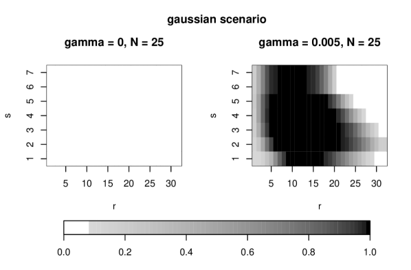
Figure 5: Empirical size (left) and power (right) of the separability test as functions of the projection set $\mathcal{I}$. The test used is $\widetilde{G}_{N}(\mathcal{I})$, with distribution approximated by the empirical bootstrap with $B=1000$. The left plot, respectively the right plot, was simulated from the Gaussian scenario with $\gamma=0$, respectively $\gamma=0.005$, and $N=25$ . Each $(r,s)$ rectangle represents the level/power of the test based on the projection set $\mathcal{I}=\left\{(i,j):1\leq i\leq r,1\leq j\leq s\right\}$.

This prompts us to investigate how the power of the test varies across all projection subsets

$$\mathcal{I}_{r,s}=\left\{(i,j):1\leq i\leq r,1\leq j\leq s\right\},$$

$r=1,\ldots,32,s=1,\ldots,7$,=. The test used is $\widetilde{G}_{N}(\mathcal{I})$, with distribution approximated by the empirical bootstrap with $B=1000$. Figure 5 shows the empirical size and power of the separability test in the Gaussian scenario for sample size $N=25$, and Figure 7, respectively Figure 8, shows the power for different sample sizes in the Gaussian scenario, respectively the non-Gaussian scenario.

4.1.1 Discussion of simulation studies

The simulation studies above illustrate how the empirical bootstrap test based on the test statistics $\widetilde{G}_{N}(\mathcal{I})$ usually outperforms its competitors, albeit it is also much more computationally expensive than the asymptotic test, whose performance are comparable in the Gaussian scenario for large enough number of observations.

The choice of the best set of eigendirections to use in the definition of the test statistics is difficult. It seems that $K$ should be ideally chosen to be increasing with $N$. This is reasonable, because larger values of $N$ increase the accuracy of the estimation of the eigenfunctions and therefore we will be able to detect departures from the separability in more eigendirections, including ones not only associated with the largest eigenvalues. However, the optimal rate at which $K$ should increase with $N$ is still an open problem, and will certainly depend in a complex way on the eigenstructure of the true underlying covariance operator $C$.

This is confirmed by the results reported in Figure 5 and Figures 7 and 8. These indeed show that taking into account too few eigendirections can result in smaller power, while including too many of them can also decrease the power.

As an alternative to tests based on projections of $D_{N}$, the tests based on the squared Hilbert–Schmidt norm of $D_{N}$, i.e. ${\left|\kern-0.86108pt\left|\kern-0.86108pt\left|D_{N}\right|\kern-0.86108pt\right|\kern-0.86108pt\right|}_{2}^{2}$, could potentially detect any departure from the separability hypothesis—as opposed to the tests $\widetilde{G}_{N}(\mathcal{I})$. But as the simulation study illustrates, they might be far less powerful in practice, particularly in situations where the departure from separability is reflected in only in a few eigendirections. Moreover, this approach still requires the computation of the full covariance operator (although not its storage) and is therefore not feasible for all applications.

4.2 Application to acoustic phonetic data

An interesting case where the proposed methods can be useful are phonetic spectrograms. These data arise in the analysis of speech records, since relevant features of recorded sounds can be better explored in a two dimensional time-frequency domain.

In particular, we consider here the dataset of 23 speakers from five different Romance languages that has been first described in Pigoli et al. (2014). The speakers were recorded while pronouncing the words corresponding to the numbers from one to ten in their language and the recordings are converted to a sampling rate of $16000$ samples per second. Since not all these words are available for all the speakers, we have a total of $219$ speech records. We focus on the spectrum that speakers produce in each speech recording $x^{L}_{ik}(t)$, where $L$ is the language, $i=1,\ldots,10$ the pronounced word and $k=1,\ldots,n_{L}$ the speaker, $n_{L}$ being the number of speakers available for language $L$. We then use a short-time Fourier transform to obtain a two dimensional log-spectrogram: we use a Gaussian window function $w(\cdot)$ with a window size of $10$ milliseconds and we compute the short-time Fourier transform as

$$X^{L}_{ik}(\omega,t)=\int_{-\infty}^{+\infty}x^{L}_{ik}(\tau)w(\tau-t)e^{-j\omega\tau}\mathrm{d}\tau.$$

The spectrogram is defined as the magnitude of the Fourier transform and the log-spectrogram (in decibel) is therefore

$$\mathfrak{S}^{L}_{ik}(\omega,t)=10\log_{10}(|X^{L}_{ik}(\omega,t)|^{2}).$$

The raw log-spectrograms are then smoothed (with the robust spline smoothing method proposed in Garcia, 2010) and aligned in time using an adaptation to 2-D of the procedure in Tang & Müller (2008). The alignment is needed because a phase distortion can be present in acoustic signals, due to difference in speech velocity between speakers. Since the different words of each language have different mean log-spectrograms, the focus of the linguistic analysis—which is the study cross-linguistics changes—is on the residual log-spectrograms

$$R_{ik}^{L}(\omega,t)=S_{ik}^{L}(\omega,t)-(1/n_{i})\sum_{k=1}^{n_{i}}S_{ik}^{L}(\omega,t).$$

Assuming that all the words within the language have the same covariance structure, we disregard hereafter the information about the pronounced words that generated the residual log-spectrogram, and use the surface data $R_{j}^{L}(\omega,t),j=1,\ldots,N_{L}$, i.e. the set of observations for the language $L$ including all speakers and words, for the separability test. These observations are measured on an equispaced grid with $81$ points in the frequency direction and $100$ points in the time direction. This translate on a full covariance structure with about $33\times 10^{6}$ degrees of freedom. Thus, although the discretized covariance matrix is in principle computable, its storage is a problem. More importantly, the accuracy of its estimate is poor, since we have at most $50$ observations within each language. For these reasons, we would like to investigate if a separable approximation of each covariance is appropriate.

We thus apply the Studentized version of the empirical bootstrap test for separability to the residual log-spectrograms for each language individually. Here, we take into consideration different choices for set of eigendirections to be used in the definition of the test statistic $\widetilde{G}_{N}(\mathcal{I})$, namely $\mathcal{I}=\mathcal{I}_{1}=\{(1,1)\}$, $\mathcal{I}=\mathcal{I}_{2}=\{(r,s):1\leq r\leq 2,1\leq s\leq 3\}$, $\mathcal{I}=\mathcal{I}_{3}=\{(r,s):1\leq r\leq 8,1\leq s\leq 10\}$. For all cases we use $B=1000$ bootstrap replicates.

The resulting $p$-values for each language and for each set of indices can be found in Table 1. Taking into account the multiple testings with a Bonferroni correction, we can conclude that the separability assumption does not appear to hold. We can also see that the departure from separability is caught mainly on the first component for the two Spanish varieties. In conclusion, a separable covariance structure is not a good fit for these languages and thus, when practitioners use this approximation for computational or modeling reasons, they should bear in mind that relevant aspects of the covariance structure may be missed in the analysis.

Table 1: $P$-values for the test for the separability of the covariance operators of the residual log-spectrograms of the five Romance languages, using the Studentized version of the empirical bootstrap.

$\mathcal{I}$	French	Italian	Portuguese	American Spanish	Iberian Spanish
$\mathcal{I}_{1}$	0.65	$<$ 0.001	$<$ 0.001	$<$ 0.001	$<$ 0.001
$\mathcal{I}_{2}$	0.078	0.197	0.022	0.36	0.013
$\mathcal{I}_{3}$	0.001	0.002	0.001	0.001	$<$ 0.001

5 Discussion and conclusions

We presented tests to verify the separability assumption for the covariance operators of random surfaces (or hypersurfaces) through hypothesis testing. These tests are based on the difference between the sample covariance operator and its separable approximation—which we have shown to be asymptotically Gaussian—projected onto subspaces spanned by the eigenfunctions of the covariance of the data. While the optimal choice for this subspace is still an open problem and it may depend on the eigenstructure of the full covariance operator, it is however possible to give some advice on how to choose $\mathcal{I}$ in practice:

• in many cases, a dimensional reduction based on the separable eigenfunctions is needed also for the follow up analysis. Then, it is recommended to use the same subspace for the test procedure as well, so that we are guaranteed at least that the projection of the covariance structure in the subspace that will be used for the analysis is separable, as shown in Section 3.

• As mentioned in Section 3, it is usually better to focus on the subset of eigenfunctions that it is possible to estimate accurately with the available data. These can be again identified with bootstrap methods such as the one described in Hall & Hosseini-Nasab (2006) or considering the dimension of the sample size. As highlighted by the results of the simulation studies in Figure 5 and in Figures 7 and 8, the empirical power of the test starts to decline when eigendirections that cannot be reasonably estimated with the available sample size are included.

• When in doubt, it is also possible to apply the test to more than one subset of eigenfunctions and then summarize the response using a Bonferroni correction. We follow this approach in the data application described in Section 4.2.

Though an asymptotic distribution is available in some cases, we also propose to approximate the distribution of our test statistics using either a parametric bootstrap (in case the distribution of the data is known) or an empirical bootstrap. A simulation study suggests that the Studentized version of the empirical bootstrap test gives the highest power in non-Gaussian settings, and has power comparable to its parametric bootstrap counterpart and to the asymptotic test in the Gaussian setting. We therefore use the Studentized empirical bootstrap for the application to linguistic data, since it is not easy to assess the distribution of the data generating process. The bootstrap test leads to the conclusion that the covariance structure is indeed not separable.

Our present approach implicitly assumed that the functional observations (e.g. the hypersurfaces) were densely observed. Though this approach is not restricted to data observed on a grid, it leaves aside the important class of functional data that are sparsely observed (e.g. Yao et al., n.d.). However, the extension of our methodology to the case of sparsely observed functional data is also possible, as long as the estimator used for the full covariance is consistent and satisfies a central limit theorem. Indeed, while we have only detailed the methods for 2-dimensional surfaces, the extension to higher-order multidimensional functions (such as 3-dimensional volumetric images from applications such as magnetic resonance imaging) is straightforward.

Appendix A The Asymptotic Covariance Structure

lemma A.1.

The covariance operator of the random operator $Z$, defined in Theorem 2.3, is characterized by the following equality, in which $\Gamma=\,\>{\mathbb{E}\left[(X\operatorname*{\otimes}X-C)\operatorname*{\>\widetilde{\bigotimes}\>}(X\operatorname*{\otimes}X-C)\right]}$:

$$\,\>{\mathbb{E}\left[\operatorname{{\mathrm{Tr}}}\left[(A_{1}\operatorname*{\>\widetilde{\otimes}\>}A_{2})Z\right]\operatorname{{\mathrm{Tr}}}\left[(B_{1}\operatorname*{\>\widetilde{\otimes}\>}B_{2})Z\right]\right]}=$$ (A.1)

$$\operatorname{{\mathrm{Tr}}}\left[(A\operatorname*{\>\widetilde{\bigotimes}\>}B)\Gamma\right]+\frac{\operatorname{{\mathrm{Tr}}}\left[BC\right]}{\operatorname{{\mathrm{Tr}}}(C)}\operatorname{{\mathrm{Tr}}}\left[(A\operatorname*{\>\widetilde{\bigotimes}\>}\mathrm{Id}_{H})\Gamma\right]-\frac{\operatorname{{\mathrm{Tr}}}[B_{2}C_{2}]}{\operatorname{{\mathrm{Tr}}}[C_{2}]}\operatorname{{\mathrm{Tr}}}\left[\left(A\operatorname*{\>\widetilde{\bigotimes}\>}(B_{1}\operatorname*{\>\widetilde{\otimes}\>}\mathrm{Id}_{H_{2}})\right)\Gamma\right]$$

$$-\frac{\operatorname{{\mathrm{Tr}}}[B_{1}C_{1}]}{\operatorname{{\mathrm{Tr}}}[C_{1}]}\operatorname{{\mathrm{Tr}}}\left[\left(A\operatorname*{\>\widetilde{\bigotimes}\>}(\mathrm{Id}_{H_{1}}\operatorname*{\>\widetilde{\otimes}\>}B_{2})\right)\Gamma\right]+\frac{\operatorname{{\mathrm{Tr}}}[AC]}{\operatorname{{\mathrm{Tr}}}[C]}\Bigg{\{}\operatorname{{\mathrm{Tr}}}\left[(\mathrm{Id}_{H}\operatorname*{\>\widetilde{\bigotimes}\>}B)\Gamma\right]+\frac{\operatorname{{\mathrm{Tr}}}[BC]}{\operatorname{{\mathrm{Tr}}}[C]}\operatorname{{\mathrm{Tr}}}[\Gamma]$$

$$-\frac{\operatorname{{\mathrm{Tr}}}[B_{2}C_{2}]}{\operatorname{{\mathrm{Tr}}}[C_{2}]}\operatorname{{\mathrm{Tr}}}\left[(\mathrm{Id}_{H}\operatorname*{\>\widetilde{\bigotimes}\>}(B_{1}\operatorname*{\>\widetilde{\otimes}\>}\mathrm{Id}_{H_{2}}))\Gamma\right]-\frac{\operatorname{{\mathrm{Tr}}}[B_{1}C_{1}]}{\operatorname{{\mathrm{Tr}}}[C_{1}]}\operatorname{{\mathrm{Tr}}}\left[(\mathrm{Id}_{H}\operatorname*{\>\widetilde{\bigotimes}\>}(\mathrm{Id}_{H_{1}}\operatorname*{\>\widetilde{\otimes}\>}B_{2}))\Gamma\right]\Bigg{\}}$$

$$-\frac{\operatorname{{\mathrm{Tr}}}[A_{2}C_{2}]}{\operatorname{{\mathrm{Tr}}}[C_{2}]}\Bigg{\{}\operatorname{{\mathrm{Tr}}}\left[\left((A_{1}\operatorname*{\>\widetilde{\otimes}\>}\mathrm{Id}_{H_{2}})\operatorname*{\>\widetilde{\bigotimes}\>}B\right)\Gamma\right]+\frac{\operatorname{{\mathrm{Tr}}}[BC]}{\operatorname{{\mathrm{Tr}}}[C]}\operatorname{{\mathrm{Tr}}}\left[\left((A_{1}\operatorname*{\>\widetilde{\otimes}\>}\mathrm{Id}_{H_{2}})\operatorname*{\>\widetilde{\bigotimes}\>}\mathrm{Id}_{H}\right)\Gamma\right]$$

$$-\frac{\operatorname{{\mathrm{Tr}}}[B_{2}C_{2}]}{\operatorname{{\mathrm{Tr}}}[C_{2}]}\operatorname{{\mathrm{Tr}}}\left[\left((A_{1}\operatorname*{\>\widetilde{\otimes}\>}\mathrm{Id}_{H_{2}})\operatorname*{\>\widetilde{\bigotimes}\>}(B_{1}\operatorname*{\>\widetilde{\otimes}\>}\mathrm{Id}_{H_{2}})\right)\Gamma\right]$$

$$-\frac{\operatorname{{\mathrm{Tr}}}[B_{1}C_{1}]}{\operatorname{{\mathrm{Tr}}}[C_{1}]}\operatorname{{\mathrm{Tr}}}\left[\left((A_{1}\operatorname*{\>\widetilde{\otimes}\>}\mathrm{Id}_{H_{2}})\operatorname*{\>\widetilde{\bigotimes}\>}(\mathrm{Id}_{H_{1}}\operatorname*{\>\widetilde{\otimes}\>}B_{2})\right)\Gamma\right]\Bigg{\}}$$

$$-\frac{\operatorname{{\mathrm{Tr}}}[A_{1}C_{1}]}{\operatorname{{\mathrm{Tr}}}[C_{1}]}\Bigg{\{}\operatorname{{\mathrm{Tr}}}\left[\left((\mathrm{Id}_{H_{1}}\operatorname*{\>\widetilde{\otimes}\>}A_{2})\operatorname*{\>\widetilde{\bigotimes}\>}B\right)\Gamma\right]+\frac{\operatorname{{\mathrm{Tr}}}[BC]}{\operatorname{{\mathrm{Tr}}}[C]}\operatorname{{\mathrm{Tr}}}\left[\left((\mathrm{Id}_{H_{1}}\operatorname*{\>\widetilde{\otimes}\>}A_{2})\operatorname*{\>\widetilde{\bigotimes}\>}\mathrm{Id}_{H}\right)\Gamma\right]$$

$$-\frac{\operatorname{{\mathrm{Tr}}}[B_{2}C_{2}]}{\operatorname{{\mathrm{Tr}}}[C_{2}]}\operatorname{{\mathrm{Tr}}}\left[\left((\mathrm{Id}_{H_{1}}\operatorname*{\>\widetilde{\otimes}\>}A_{2})\operatorname*{\>\widetilde{\bigotimes}\>}(B_{1}\operatorname*{\>\widetilde{\otimes}\>}\mathrm{Id}_{H_{2}})\right)\Gamma\right]$$

$$-\frac{\operatorname{{\mathrm{Tr}}}[B_{1}C_{1}]}{\operatorname{{\mathrm{Tr}}}[C_{1}]}\operatorname{{\mathrm{Tr}}}\left[\left((\mathrm{Id}_{H_{1}}\operatorname*{\>\widetilde{\otimes}\>}A_{2})\operatorname*{\>\widetilde{\bigotimes}\>}(\mathrm{Id}_{H_{1}}\operatorname*{\>\widetilde{\otimes}\>}B_{2})\right)\Gamma\right]\Bigg{\}},$$

where $A_{1},B_{1}\in\mathcal{S}_{\infty}(H_{1}),A_{2},B_{2}\in\mathcal{S}_{\infty}(H_{2})$, and $A=A_{1}\operatorname*{\>\widetilde{\otimes}\>}A_{2}$, $B=B_{1}\operatorname*{\>\widetilde{\otimes}\>}B_{2}$, $H=H_{1}\operatorname*{\otimes}H_{2}$, and $\mathrm{Id}_{H}$ denotes the identity operator on the Hilbert space $H$.

Proof.

By the linearity of the expectation and the trace, and by the properties of the partial trace, the computation of (A.1) boils down to the computation of expressions of the form

$$\,\>{\mathbb{E}\left[\operatorname{{\mathrm{Tr}}}\left[(A^{\prime}_{1}\operatorname*{\>\widetilde{\otimes}\>}A^{\prime}_{2})Y\right]\operatorname{{\mathrm{Tr}}}\left[(B^{\prime}_{1}\operatorname*{\>\widetilde{\otimes}\>}B^{\prime}_{2})Y\right]\right]},$$

for general $A^{\prime}_{1},B^{\prime}_{1}\in\mathcal{S}_{\infty}(H_{1}),A^{\prime}_{2},B^{\prime}_{2}\in\mathcal{S}_{\infty}(H_{2})$. Since $\operatorname{\>{\mathbb{E}}}{\left|\kern-0.77498pt\left|\kern-0.77498pt\left|Y\right|\kern-0.77498pt\right|\kern-0.77498pt\right|}_{1}^{2}<\infty$, we have

$$\operatorname{\>{\mathbb{E}}}{(\operatorname{{\mathrm{Tr}}}\left[(A^{\prime}_{1}\operatorname*{\>\widetilde{\otimes}\>}A^{\prime}_{2})Y\right]\operatorname{{\mathrm{Tr}}}\left[(B^{\prime}_{1}\operatorname*{\>\widetilde{\otimes}\>}B^{\prime}_{2})Y\right])}=$$

$$=\operatorname{{\mathrm{Tr}}}\left[\left((A^{\prime}_{1}\operatorname*{\>\widetilde{\otimes}\>}A^{\prime}_{2})\operatorname*{\>\widetilde{\bigotimes}\>}(B^{\prime}_{1}\operatorname*{\>\widetilde{\otimes}\>}B^{\prime}_{2})\right)\operatorname{\>{\mathbb{E}}}{\left(Y\operatorname*{\>\widetilde{\bigotimes}\>}Y\right)}\right]$$

$$=\operatorname{{\mathrm{Tr}}}\left[\left((A^{\prime}_{1}\operatorname*{\>\widetilde{\otimes}\>}A^{\prime}_{2})\operatorname*{\>\widetilde{\bigotimes}\>}(B^{\prime}_{1}\operatorname*{\>\widetilde{\otimes}\>}B^{\prime}_{2})\right)\Gamma\right],$$

where $\Gamma=\,\>{\mathbb{E}\left[(X\operatorname*{\otimes}X-C)\operatorname*{\>\widetilde{\bigotimes}\>}(X\operatorname*{\otimes}X-C)\right]}$. The computation of (A.1) follows directly. ∎

Appendix B Proofs

Proof of Corollary 2.4.

To alleviate the notation, we shall assume without loss of generality that $\mu=\operatorname{\>{\mathbb{E}}}X=0$. Using the properties of the tensor product (see Appendix D.1, we get that $T_{N}(r,s)=\operatorname{{\mathrm{Tr}}}\left[(\hat{A}_{r}\operatorname*{\>\widetilde{\otimes}\>}\hat{B}_{s})\sqrt{N}D_{N}\right]$, where $\hat{A}_{r}=(\hat{u}_{r}\operatorname*{\otimes_{2}}\hat{u}_{r})$, $\hat{B}_{s}=(\hat{v}_{s}\operatorname*{\otimes_{2}}\hat{v}_{s})$. Now notice that though $A_{r}=u_{r}\operatorname*{\otimes_{2}}u_{r}$ and $B_{s}=v_{s}\operatorname*{\otimes_{2}}v_{s}$ are not estimable separately (since $C_{1}$ and $C_{2}$ are not identifiable), their $\operatorname*{\>\widetilde{\otimes}\>}$-product is identifiable, and is consistently estimated by $\hat{A}_{r}\operatorname*{\>\widetilde{\otimes}\>}\hat{B}_{s}$ (in trace norm). Slutsky’s Lemma, Theorem 2.3 and the continuous mapping theorem imply therefore that $\left(T_{N}(r,s)\right)_{(r,s)\in\mathcal{I}}$ has the same asymptotic distribution of $\left(\widetilde{T}_{N}(r,s)\right)_{(r,s)\in\mathcal{I}}$, where $\widetilde{T}_{N}(r,s)=\operatorname{{\mathrm{Tr}}}\left[(A_{r}\operatorname*{\>\widetilde{\otimes}\>}B_{s})\sqrt{N}D_{N}\right]$. This implies that

$$\left(T_{N}(r,s)\right)_{(r,s)\in\mathcal{I}}\stackrel{{\scriptstyle d}}{{\longrightarrow}}Z^{\prime}=\left(\operatorname{{\mathrm{Tr}}}\left[(A_{r}\operatorname*{\>\widetilde{\otimes}\>}B_{s})Z\right]\right)_{(r,s)\in\mathcal{I}},\quad\text{as }N\rightarrow\infty,$$

where $Z$ is a mean zero Gaussian random element of $\mathcal{S}_{1}(H_{1}\operatorname*{\otimes}H_{2})$ whose covariance structure is given by Lemma A.1. $Z^{\prime}$ is therefore also Gaussian random element, with mean zero and covariances

$$\Sigma_{(r,s),(r^{\prime},s^{\prime})}=\operatorname{{\mathrm{cov}}}(Z^{\prime}_{(r,s)},Z^{\prime}_{(r^{\prime},s^{\prime})})=\,\>{\mathbb{E}\left[\operatorname{{\mathrm{Tr}}}\left[(A_{r}\operatorname*{\>\widetilde{\otimes}\>}B_{s})Z\right]\operatorname{{\mathrm{Tr}}}\left[A_{r^{\prime}}\operatorname*{\>\widetilde{\otimes}\>}B_{s^{\prime}})Z\right]\right]}.$$

Using Lemma A.1, we see that the computation of $\Sigma_{(r,s),(r^{\prime},s^{\prime})}$ depends on the terms $\operatorname{{\mathrm{Tr}}}\left[(A_{r}\operatorname*{\>\widetilde{\otimes}\>}B_{s})C\right]=\lambda_{r}\gamma_{s}$, $\operatorname{{\mathrm{Tr}}}\left[A_{r}C_{1}\right]=\lambda_{r}$, $\operatorname{{\mathrm{Tr}}}\left[B_{s}C_{2}\right]=\gamma_{s}$, as well as on the value of

$$\operatorname{{\mathrm{Tr}}}\left[\left((A_{1}^{\prime}\operatorname*{\>\widetilde{\otimes}\>}B_{1}^{\prime})\operatorname*{\>\widetilde{\bigotimes}\>}(A_{2}^{\prime}\operatorname*{\>\widetilde{\otimes}\>}B_{2}^{\prime})\right)\Gamma\right]$$

for general $A_{1}^{\prime},A_{2}^{\prime}\in\mathcal{S}_{\infty}(H_{1}),B_{1}^{\prime},B_{2}^{\prime}\in\mathcal{S}_{\infty}(H_{2})$. Using the Karhunen–Loève expansion $X=\sum_{i,i^{\prime}\geq 1}\xi_{ii^{\prime}}u_{i}\operatorname*{\otimes}v_{i^{\prime}}$, where $\xi_{ii^{\prime}}=\left\langle X,u_{i}\operatorname*{\otimes}v_{i^{\prime}}\right\rangle$, we get

$$\Gamma =\operatorname{\>{\mathbb{E}}}\left(\left(X\operatorname*{\otimes_{2}}X-C\right)\operatorname*{\>\widetilde{\otimes}\>}\left(X\operatorname*{\otimes_{2}}X-C\right)\right)$$

$$=\sum_{i,i^{\prime},j,j^{\prime},k,k^{\prime},l,l^{\prime}\geq 1}\beta_{ii^{\prime}jj^{\prime}kk^{\prime}ll^{\prime}}\left(u_{ij}\operatorname*{\>\widetilde{\otimes}\>}v_{i^{\prime}j^{\prime}}\right)\operatorname*{\>\widetilde{\bigotimes}\>}\left(u_{kl}\operatorname*{\>\widetilde{\otimes}\>}v_{k^{\prime}l^{\prime}}\right)$$

$$\qquad-\sum_{i,i^{\prime},j,j^{\prime}}\alpha_{ii^{\prime}}\alpha_{jj^{\prime}}\left(u_{ii}\operatorname*{\>\widetilde{\otimes}\>}v_{i^{\prime}i^{\prime}}\right)\operatorname*{\>\widetilde{\bigotimes}\>}\left(u_{jj}\operatorname*{\>\widetilde{\otimes}\>}v_{j^{\prime}j^{\prime}}\right)$$

where we have written $u_{ij}=u_{i}\operatorname*{\otimes_{2}}u_{j}\in\mathcal{S}_{1}(H_{1}),v_{ij}=v_{i}\operatorname*{\otimes_{2}}v_{j}\in\mathcal{S}_{1}(H_{2})$, $\beta_{ii^{\prime}jj^{\prime}kk^{\prime}ll^{\prime}}=\,\>{\mathbb{E}\left[\xi_{ii^{\prime}}\xi_{jj^{\prime}}\xi_{kk^{\prime}}\xi_{ll^{\prime}}\right]}$, $\alpha_{ij}=\lambda_{i}\gamma_{j}$ and used the identity $u_{ij}\operatorname*{\>\widetilde{\otimes}\>}v_{i^{\prime}j^{\prime}}=(u_{i}\operatorname*{\otimes}v_{i^{\prime}})\operatorname*{\otimes_{2}}(u_{j}\operatorname*{\otimes}v_{j^{\prime}})$. Therefore,

$$\operatorname{{\mathrm{Tr}}}\left[\left((A_{1}^{\prime}\operatorname*{\>\widetilde{\otimes}\>}A_{2}^{\prime})\operatorname*{\>\widetilde{\bigotimes}\>}(B_{1}^{\prime}\operatorname*{\>\widetilde{\otimes}\>}B_{2}^{\prime})\right)\Gamma\right]=$$

$$=\sum_{i,i^{\prime},j,j^{\prime},k,k^{\prime},l,l^{\prime}\geq 1}\beta_{ii^{\prime}jj^{\prime}kk^{\prime}ll^{\prime}}\operatorname{{\mathrm{Tr}}}[A_{1}^{\prime}u_{ij}]\operatorname{{\mathrm{Tr}}}[A_{2}^{\prime}v_{i^{\prime}j^{\prime}}]\operatorname{{\mathrm{Tr}}}[B_{1}^{\prime}u_{kl}]\operatorname{{\mathrm{Tr}}}[B_{2}^{\prime}v_{k^{\prime}l^{\prime}}]$$

$$\qquad-\sum_{i,i^{\prime},j,j^{\prime}}\alpha_{ii^{\prime}}\alpha_{jj^{\prime}}\operatorname{{\mathrm{Tr}}}[A_{1}^{\prime}u_{ii}]\operatorname{{\mathrm{Tr}}}[B_{1}^{\prime}u_{jj}]\operatorname{{\mathrm{Tr}}}[A_{2}^{\prime}v_{i^{\prime}i^{\prime}}]\operatorname{{\mathrm{Tr}}}[B_{2}^{\prime}v_{j^{\prime}j^{\prime}}],$$

and the computation of the variance $\Sigma_{(r,s),(r^{\prime},s^{\prime})}$ follows from a straightforward (though tedious) calculation. ∎

Proof of Corollary 2.5.

We only need to compute and substitute the values of the fourth order moments terms $\tilde{\beta}_{ijkl}$ in the expression given by Corollary 2.4. Since $\tilde{\beta}_{ijkl}=\,\>{\mathbb{E}\left[\xi_{ij}^{2}\xi_{kl}^{2}\right]}=3\alpha_{kl}^{2}$ if $(i,j)=(k,l)$, and $\tilde{\beta}_{ijkl}=\alpha_{ij}\alpha_{kl}$ if $(i,j)\neq(k,l)$, straightforward calculations give

$$\tilde{\beta}_{rs\cdot\cdot} =2\alpha_{rs}^{2}+\alpha_{rs}\operatorname{{\mathrm{Tr}}}(C)=\tilde{\beta}_{r\cdot\cdot s}, \tilde{\beta}_{\cdot\cdot\cdot\cdot} =\operatorname{{\mathrm{Tr}}}(C)^{2}+2{\left|\kern-0.77498pt\left|\kern-0.77498pt\left|C\right|\kern-0.77498pt\right|\kern-0.77498pt\right|}_{2}^{2},$$

$$\tilde{\beta}_{\cdot s\cdot s^{\prime}} =\gamma_{s}\gamma_{s^{\prime}}(\operatorname{{\mathrm{Tr}}}(C_{1})^{2}+2\delta_{ss^{\prime}}{\left|\kern-0.77498pt\left|\kern-0.77498pt\left|C_{1}\right|\kern-0.77498pt\right|\kern-0.77498pt\right|}_{2}^{2}), \tilde{\beta}_{r\cdot r^{\prime}\cdot} =\lambda_{r}\lambda_{r^{\prime}}(\operatorname{{\mathrm{Tr}}}(C_{2})^{2}+2\delta_{rr^{\prime}}{\left|\kern-0.77498pt\left|\kern-0.77498pt\left|C_{2}\right|\kern-0.77498pt\right|\kern-0.77498pt\right|}_{2}^{2}),$$

$$\tilde{\beta}_{rs\cdot s^{\prime}} =2\delta_{ss^{\prime}}\alpha_{rs}^{2}+\alpha_{rs}\gamma_{s^{\prime}}\operatorname{{\mathrm{Tr}}}(C_{1}), \tilde{\beta}_{rsr^{\prime}\cdot} =2\delta_{rr^{\prime}}\alpha_{rs}^{2}+\alpha_{rs}\lambda_{r^{\prime}}\operatorname{{\mathrm{Tr}}}(C_{2}),$$

$$\tilde{\beta}_{\cdot\cdot\cdot s} =2\gamma_{s}^{2}{\left|\kern-0.77498pt\left|\kern-0.77498pt\left|C_{1}\right|\kern-0.77498pt\right|\kern-0.77498pt\right|}_{2}^{2}+\gamma_{s}\operatorname{{\mathrm{Tr}}}(C_{1})^{2}\operatorname{{\mathrm{Tr}}}(C_{2}), \tilde{\beta}_{r\cdot\cdot\cdot} =2\lambda_{r}^{2}{\left|\kern-0.77498pt\left|\kern-0.77498pt\left|C_{2}\right|\kern-0.77498pt\right|\kern-0.77498pt\right|}_{2}^{2}+\lambda_{r}\operatorname{{\mathrm{Tr}}}(C_{1})\operatorname{{\mathrm{Tr}}}(C_{2})^{2},$$

where $\delta_{ij}=1$ if $i=j$, and zero otherwise. The proof is finished by direct calculations. ∎

Appendix C Partial Traces

Letting $\mathcal{S}_{1}(H_{1}\operatorname*{\otimes}H_{2})$ denote the space of trace-class operators on $H_{1}\operatorname*{\otimes}H_{2}$, we define the partial trace with respect to $H_{1}$ as the unique linear operator $\operatorname{{\mathrm{Tr}}}_{1}:\mathcal{S}_{1}(H_{1}\operatorname*{\otimes}H_{2})\rightarrow\mathcal{S}_{1}(H_{2})$ satisfying $\operatorname{{\mathrm{Tr}}}_{1}(A\operatorname*{\>\widetilde{\otimes}\>}B)=\operatorname{{\mathrm{Tr}}}(A)B$ for all $A\in\mathcal{S}_{1}(H_{1})$, $B\in\mathcal{S}_{1}(H_{2})$.

proposition C.1.

The operator $\operatorname{{\mathrm{Tr}}}_{1}$ is well-defined, linear, continuous, and satisfies

$${\left|\kern-0.77498pt\left|\kern-0.77498pt\left|\operatorname{{\mathrm{Tr}}}_{1}(A)\right|\kern-0.77498pt\right|\kern-0.77498pt\right|}_{1}\leq{\left|\kern-0.77498pt\left|\kern-0.77498pt\left|A\right|\kern-0.77498pt\right|\kern-0.77498pt\right|}_{1},\quad A\in\mathcal{S}_{1}(H_{1}\operatorname*{\otimes}H_{2})$$ (C.1)

Furthermore,

$$\operatorname{{\mathrm{Tr}}}(S\operatorname{{\mathrm{Tr}}}_{1}(T))=\operatorname{{\mathrm{Tr}}}((\mathrm{Id}_{1}\operatorname*{\>\widetilde{\otimes}\>}S)T),\qquad T\in\mathcal{S}_{1}(H_{1}\operatorname*{\otimes}H_{2}),S\in\mathcal{S}_{\infty}(H_{2}),$$ (C.2)

where $\mathrm{Id}_{1}$ is the identity operator on $H_{1}$.

Proof.

Let us start by proving that the operator $\operatorname{{\mathrm{Tr}}}_{1}(\cdot)$ is well defined. By Lemma D.6, the space

$$B_{0}=\{\sum_{i=1}^{n}A_{i}\operatorname*{\>\widetilde{\otimes}\>}B_{i}:A_{i}\in\mathcal{S}_{1}(H_{1}),B_{i}\in\mathcal{S}_{1}(H_{2}),n=1,2,\ldots\}$$

is a dense subset of $\mathcal{S}_{1}(H_{1}\operatorname*{\otimes}H_{2})$. We therefore only need to show that $\operatorname{{\mathrm{Tr}}}_{1}(\cdot)$ is continuous on $B_{0}$. Let $T\in B_{0}$, $T=\sum_{i=1}^{n}A_{i}\operatorname*{\>\widetilde{\otimes}\>}B_{i}$. Then, for any $S\in\mathcal{S}_{\infty}(H_{2})$, we have

$$\operatorname{{\mathrm{Tr}}}(S\operatorname{{\mathrm{Tr}}}_{1}(T)) =\sum_{i=1}^{n}\operatorname{{\mathrm{Tr}}}(A_{i})\operatorname{{\mathrm{Tr}}}(SB_{i})=\sum_{i=1}^{n}\operatorname{{\mathrm{Tr}}}\left((\mathrm{Id}_{1}\operatorname*{\>\widetilde{\otimes}\>}S)(A_{i}\operatorname*{\>\widetilde{\otimes}\>}B_{i})\right)=$$

$$=\operatorname{{\mathrm{Tr}}}\left((\mathrm{Id}_{1}\operatorname*{\>\widetilde{\otimes}\>}S)\left[\sum_{i=1}^{n}A_{i}\operatorname*{\>\widetilde{\otimes}\>}B_{i}\right]\right)=\operatorname{{\mathrm{Tr}}}\left((\mathrm{Id}_{1}\operatorname*{\>\widetilde{\otimes}\>}S)T\right).$$

Hence, using the following formula for the trace norm,

$${\left|\kern-0.77498pt\left|\kern-0.77498pt\left|T\right|\kern-0.77498pt\right|\kern-0.77498pt\right|}_{1}=\sup\left\{|\operatorname{{\mathrm{Tr}}}(ST)|:{\left|\kern-0.77498pt\left|\kern-0.77498pt\left|S\right|\kern-0.77498pt\right|\kern-0.77498pt\right|}_{\infty}=1\right\},$$

we get ${\left|\kern-0.77498pt\left|\kern-0.77498pt\left|\operatorname{{\mathrm{Tr}}}_{1}(T)\right|\kern-0.77498pt\right|\kern-0.77498pt\right|}_{1}\leq{\left|\kern-0.77498pt\left|\kern-0.77498pt\left|T\right|\kern-0.77498pt\right|\kern-0.77498pt\right|}_{1}$ for all $T\in B_{0}$. Thus $\operatorname{{\mathrm{Tr}}}_{1}(\cdot)$ can be extended by continuity to $H_{1}\operatorname*{\otimes}H_{2}$, and (C.1) (of the paper) holds.

Let us now show (C.2) (of the paper). Fix $S\in\mathcal{S}_{\infty}(H_{2})$, and define the linear functionals $g_{S},h_{S}:\mathcal{S}_{1}(H_{1}\operatorname*{\otimes}H_{2})\rightarrow\mathbb{R}$ by $g_{S}(T)=\operatorname{{\mathrm{Tr}}}\left((S\operatorname*{\>\widetilde{\otimes}\>}\mathrm{Id}_{2})T\right)$ and $h_{S}(T)=\operatorname{{\mathrm{Tr}}}(S\operatorname{{\mathrm{Tr}}}_{1}(T))$, for $T\in\mathcal{S}_{1}(H_{1}\operatorname*{\otimes}H_{2})$. By Hölder’s inequality and (C.1) (of the paper), $g_{S}$ and $h_{S}$ are both continuous. Since they are equal on the dense subset $B_{0}$, they are in fact equal everywhere, and (C.2) (of the paper) follows. ∎

We can also define $\operatorname{{\mathrm{Tr}}}_{2}:\mathcal{S}_{1}(H_{1}\operatorname*{\otimes}H_{2})\rightarrow\mathcal{S}_{1}(H_{1})$ analogously. The following result gives an explicit formula for the partial traces of integral operators with continuous kernels.

proposition C.2.

Let $D_{s}\subset\mathbb{R}^{p},D_{t}\subset\mathbb{R}^{q}$ be compact subsets, $H_{1}=L^{2}\left(D_{s},\mathbb{R}\right),H_{2}=L^{2}\left(D_{t},\mathbb{R}\right)$, and $H=L^{2}(D_{s}\times D_{t},\mathbb{R})=H_{1}\operatorname*{\otimes}H_{2}$. If $C\in\mathcal{S}_{1}(L^{2}(D_{s}\times D_{t},\mathbb{R}))$ is a positive definite operator with symmetric continuous kernel $c=c(s,t,s^{\prime},t^{\prime})$, i.e. $c(s,t,s^{\prime},t^{\prime})=c(s^{\prime},t^{\prime},s,t)$ for all $s,s^{\prime}\in D_{s},t,t^{\prime}\in D_{t}$, and

$$Cf(s,t)=\iint_{D_{s}\times D_{t}}c(s,t,s^{\prime},t^{\prime})f(s^{\prime},t^{\prime})ds^{\prime}dt^{\prime},\qquad f\in L^{2}(D_{s}\times D_{t},\mathbb{R}),$$

then $\operatorname{{\mathrm{Tr}}}_{1}(C)$ is the integral operator on $L^{2}(D_{t},\mathbb{R})$ with kernel $k(t,t^{\prime})=\int_{D_{s}}c(s,t,s,t^{\prime})ds$. The analogous result also holds for $\operatorname{{\mathrm{Tr}}}_{2}(C)$.

Proof.

Let ${\varepsilon}>0$. By Lemma D.7, we know that there exists an integral operator $C^{\prime}$ with continuous kernel $c^{\prime}$ such that ${\left|\kern-0.77498pt\left|\kern-0.77498pt\left|C-C^{\prime}\right|\kern-0.77498pt\right|\kern-0.77498pt\right|}_{1}\leq{\varepsilon}/2$ and ${\left\lVert c-c^{\prime}\right\rVert}_{\infty}\leq{\varepsilon}/2,$ where $C^{\prime}=\sum_{n=1}^{N}A_{n}\operatorname*{\>\widetilde{\otimes}\>}B_{n}$, and each $A_{n},B_{n}$ are finite rank operators, with continuous kernels $a_{n}$, respectively $b_{n}$, and ${\left\lVert g\right\rVert}_{\infty}\leavevmode\nobreak\ =\leavevmode\nobreak\ \sup_{x}|g(x)|$. We have

$${\left|\kern-0.77498pt\left|\kern-0.77498pt\left|\operatorname{{\mathrm{Tr}}}_{1}(C)-\int_{D_{s}}c(s,\cdot,s,\cdot)ds\right|\kern-0.77498pt\right|\kern-0.77498pt\right|}_{2} \leq{\left|\kern-0.77498pt\left|\kern-0.77498pt\left|\operatorname{{\mathrm{Tr}}}_{1}(C)-\operatorname{{\mathrm{Tr}}}_{1}(C^{\prime})\right|\kern-0.77498pt\right|\kern-0.77498pt\right|}_{2}$$ (C.3)

$$\quad+{\left|\kern-0.77498pt\left|\kern-0.77498pt\left|\operatorname{{\mathrm{Tr}}}_{1}(C^{\prime})-\int_{D_{s}}c^{\prime}(s,\cdot,s,\cdot)ds\right|\kern-0.77498pt\right|\kern-0.77498pt\right|}_{2}$$

$$\quad+{\left|\kern-0.77498pt\left|\kern-0.77498pt\left|\int_{D_{s}}c^{\prime}(s,\cdot,s,\cdot)ds-\int_{D_{s}}c(s,\cdot,s,\cdot)ds\right|\kern-0.77498pt\right|\kern-0.77498pt\right|}_{2}.$$

The first term is bounded ${\left|\kern-0.77498pt\left|\kern-0.77498pt\left|\operatorname{{\mathrm{Tr}}}_{1}(C)-\operatorname{{\mathrm{Tr}}}_{1}(C^{\prime})\right|\kern-0.77498pt\right|\kern-0.77498pt\right|}_{1}\leq{\left|\kern-0.77498pt\left|\kern-0.77498pt\left|C-C^{\prime}\right|\kern-0.77498pt\right|\kern-0.77498pt\right|}_{1}\leq{\varepsilon}/2$. The second term is equal to zero since

$$\operatorname{{\mathrm{Tr}}}_{1}(\sum_{n=1}^{N}A_{n}\operatorname*{\>\widetilde{\otimes}\>}B_{n}) =\sum_{n=1}^{N}\operatorname{{\mathrm{Tr}}}(A_{n})B_{n}$$

$$=\sum_{n=1}^{N}\int_{D_{s}}A_{n}(s,s)dsB_{n}$$

$$=\int_{D_{s}}\left(\sum_{n=1}^{N}A_{n}\operatorname*{\>\widetilde{\otimes}\>}B_{n}\right)(s,\cdot,s,\cdot)ds.$$

$$=\int_{D_{s}}c^{\prime}(s,\cdot,s,\cdot)ds,$$

where the second equality comes from the fact that $A_{n}$ is a finite rank operator (hence trace-class) with continuous kernel. The third term of (C.3) is

$$\left(\iint_{D_{t}\times D_{t}}\left(\int_{D_{s}}\left[c^{\prime}(s,t,s,t^{\prime})-c(s,t,s,t^{\prime})\right]ds\right)^{2}dtdt^{\prime}\right)^{1/2}\\ \leq|D_{s}|\>|D_{t}|\>{\left\lVert c^{\prime}-c\right\rVert}_{\infty}\leq{\varepsilon}/2,$$

where $|D_{s}|=\int_{D_{s}}dx$ and $|D_{t}|=\int_{D_{t}}dy$. Therefore,

$${\left|\kern-0.77498pt\left|\kern-0.77498pt\left|\operatorname{{\mathrm{Tr}}}_{1}(C)-\int_{D_{s}}c(s,t,s,t^{\prime})ds\right|\kern-0.77498pt\right|\kern-0.77498pt\right|}_{2}\leq{\varepsilon}.$$

Since this holds for any ${\varepsilon}>0$, $\operatorname{{\mathrm{Tr}}}_{1}(C)$ is equal to the operator with kernel $k(t,t^{\prime})=\int_{D_{s}}c(s,t,s,t^{\prime})ds$. The proof of the analogous result for $\operatorname{{\mathrm{Tr}}}_{2}(C)$ is similar. ∎

The next result states that the partial trace of a Gaussian random trace-class operator is also Gaussian.

proposition C.3.

Let $Z\in\mathcal{S}_{1}(H_{1}\operatorname*{\otimes}H_{2})$ be a Gaussian random element. Then $\operatorname{{\mathrm{Tr}}}_{1}(Z)\in\mathcal{S}_{1}(H_{2})$ is a Gaussian random element.

Proof.

The proof is finished by noticing that $A\in\mathcal{S}_{\infty}(H_{2})$, we have $\operatorname{{\mathrm{Tr}}}(A\operatorname{{\mathrm{Tr}}}_{1}(Z))=\operatorname{{\mathrm{Tr}}}\left((\mathrm{Id}\operatorname*{\>\widetilde{\otimes}\>}A)Z\right)$, where the right-hand side is obviously Gaussian. ∎

Appendix D Background Results

This section presents some background results that are used in the paper. Some references for these results are Zhu (2007); Gohberg & Krejn (1971); Gohberg et al. (1990); Kadison & Ringrose (1997a, b); Ringrose (1971).

D.1 Tensor Products Hilbert Spaces, and Hilbert–Schmidt Operators

Let $H_{1},H_{2}$ be two real separable Hilbert spaces, whose inner products are denoted by $\left\langle\cdot,\cdot\right\rangle_{1}$ and $\left\langle\cdot,\cdot\right\rangle_{2}$, respectively. Let $H_{1}\operatorname*{\otimes}H_{2}$ denote the Hilbert space obtained as the completion of the space of finite linear combinations of simple tensors $u\operatorname*{\otimes}v,u\in H_{1},v\in H_{2}$ under the inner product

$$\left\langle u\operatorname*{\otimes}v,u^{\prime}\operatorname*{\otimes}v^{\prime}\right\rangle=\left\langle u,u^{\prime}\right\rangle_{1}\left\langle v,v^{\prime}\right\rangle_{2}.$$

The Hilbert space $H_{1}\operatorname*{\otimes}H_{2}$ is actually isometrically isomorphic to the space of Hilbert–Schmidt operators from $H_{2}$ to $H_{1}$, denoted by $\mathcal{S}_{2}(H_{2},H_{1})$, which consists of all continuous linear operators $T:H_{2}\rightarrow H_{1}$ satisfying

$${\left|\kern-0.77498pt\left|\kern-0.77498pt\left|T\right|\kern-0.77498pt\right|\kern-0.77498pt\right|}_{2}^{2}=\sum_{n\geq 1}{\left\lVert Te_{n}\right\rVert}^{2},$$

where the sum extends over any orthonormal basis $(e_{n})_{n\geq 1}$ of $H_{2}$. The norm ${\left|\kern-0.77498pt\left|\kern-0.77498pt\left|\cdot\right|\kern-0.77498pt\right|\kern-0.77498pt\right|}$ is actually induced by the inner-product inner product

$$\left\langle T,S\right\rangle_{\!\!\mathcal{S}_{2}}=\sum_{n\geq 1}\left\langle Te_{n},Se_{n}\right\rangle_{1},\quad T,S\in\mathcal{S}_{2}(H_{2},H_{1}),$$

which is independent of the choice of the basis (the space $\mathcal{S}_{2}(H_{2},H_{1})$ is therefore itself a Hilbert space). The isomorphism between $H_{1}\operatorname*{\otimes}H_{2}$ and $\mathcal{S}_{2}(H_{2},H_{1})$ is given by the mapping $\Phi:H_{1}\operatorname*{\otimes}H_{2}\rightarrow\mathcal{S}_{2}(H_{2},H_{1})$, defined by $\Phi(u\operatorname*{\otimes}v)=u\operatorname*{\otimes_{2}}v$ for all $u\in H_{1},v\in H_{2}$, where $u\operatorname*{\otimes_{2}}v(v^{\prime})=\left\langle v^{\prime},v\right\rangle u$ for $u\in H_{1},v,v^{\prime}\in H_{2}$. We therefore identify these two spaces, and might write $u\operatorname*{\otimes}v$ instead of $u\operatorname*{\otimes_{2}}v$ hereafter.

Notice that since $\mathcal{H}=\mathcal{S}_{2}(H_{1})=\mathcal{S}_{2}(H_{1},H_{1})$ is itself a Hilbert space, if $A,B\in\mathcal{H}$, the operator $A\operatorname*{{\bigotimes}_{2}}B\in\mathcal{S}_{2}(\mathcal{H},\mathcal{H})$ is defined by $\left(A\operatorname*{{\bigotimes}_{2}}B\right)(C)=\left\langle C,B\right\rangle_{\!\!\mathcal{S}_{2}}A$, for $A,B,C\in\mathcal{H}$. Here are some properties of the tensor product $\cdot\operatorname*{\otimes_{2}}\cdot$:

proposition D.1.

Let $H$ be a real separable Hilbert space. For any $u,v,f,g\in H$, $A,B\in\mathcal{S}_{2}(H)$

1. $\cdot\operatorname*{\otimes_{2}}\cdot$ is linear on the left, and conjugate-linear on the right,

2. $\left\langle u\operatorname*{\otimes_{2}}v,f\operatorname*{\otimes_{2}}g\right\rangle_{\!\!\mathcal{S}_{2}}=\left\langle u,f\right\rangle\left\langle g,v\right\rangle=\left\langle(u\operatorname*{\otimes_{2}}v)g,f\right\rangle$,

3. $\left\langle A,u\operatorname*{\otimes_{2}}v\right\rangle_{\!\!\mathcal{S}_{2}}=\left\langle Av,u\right\rangle=\left\langle v\operatorname*{\otimes_{2}}u,A^{{\dagger}}\right\rangle_{\!\!\mathcal{S}_{2}},$

4. $\operatorname{{\mathrm{Tr}}}(u\operatorname*{\otimes_{2}}v)=\left\langle u,v\right\rangle$,

5. ${\left|\kern-0.77498pt\left|\kern-0.77498pt\left|u\operatorname*{\otimes_{2}}v\right|\kern-0.77498pt\right|\kern-0.77498pt\right|}_{1}={\left|\kern-0.77498pt\left|\kern-0.77498pt\left|u\operatorname*{\otimes_{2}}v\right|\kern-0.77498pt\right|\kern-0.77498pt\right|}_{2}={\left\lVert u\right\rVert}{\left\lVert v\right\rVert}$,

6. $(u\operatorname*{\otimes_{2}}v)(f\operatorname*{\otimes_{2}}g)=\left\langle f,v\right\rangle u\operatorname*{\otimes_{2}}g$,

7. $(u\operatorname*{\otimes_{2}}v)^{{\dagger}}=v\operatorname*{\otimes_{2}}u,$

8. $(A\operatorname*{{\bigotimes}_{2}}B)^{{\dagger}}=B\operatorname*{{\bigotimes}_{2}}A$.

Proof.

The proof follows from the definition and the properties of the inner product, and is therefore omitted. ∎

Recall that for $A\in\mathcal{S}_{\infty}(H_{1}),B\in\mathcal{S}_{\infty}(H_{2})$, the operator $(A\operatorname*{\>\widetilde{\otimes}\>}B)\in\mathcal{S}_{\infty}(H_{1}\operatorname*{\otimes}H_{2})$ is defined by the linear extension of

$$(A\operatorname*{\>\widetilde{\otimes}\>}B)(u\operatorname*{\otimes}v)=Au\operatorname*{\otimes}Bv,u\in H_{1},v\in H_{2}$$

Furthermore, we have $(A\operatorname*{\>\widetilde{\otimes}\>}B)^{{\dagger}}=A^{{\dagger}}\operatorname*{\>\widetilde{\otimes}\>}B^{{\dagger}}$, ${\left|\kern-0.77498pt\left|\kern-0.77498pt\left|A\operatorname*{\>\widetilde{\otimes}\>}B\right|\kern-0.77498pt\right|\kern-0.77498pt\right|}_{\infty}={\left|\kern-0.77498pt\left|\kern-0.77498pt\left|A\right|\kern-0.77498pt\right|\kern-0.77498pt\right|}_{\infty}{\left|\kern-0.77498pt\left|\kern-0.77498pt\left|B\right|\kern-0.77498pt\right|\kern-0.77498pt\right|}_{\infty}$, and $(A\operatorname*{\>\widetilde{\otimes}\>}B)(C\operatorname*{\>\widetilde{\otimes}\>}D)=(AC\operatorname*{\>\widetilde{\otimes}\>}CD)$ for $A,C\in\mathcal{S}_{\infty}(H_{1})$, $B,D\in\mathcal{S}_{\infty}(H_{2})$. For $u,v\in H_{1},f,g\in H_{2}$, $(u\operatorname*{\otimes_{2}}v)\operatorname*{\>\widetilde{\otimes}\>}(f\operatorname*{\otimes_{2}}g)=(u\operatorname*{\otimes}f)\operatorname*{{\bigotimes}_{2}}(v\operatorname*{\otimes}g)$ If $A\in\mathcal{S}_{1}(H_{1}),B\in\mathcal{S}_{1}(H_{2})$, then $A\operatorname*{\>\widetilde{\otimes}\>}B\in\mathcal{S}_{1}(H_{1}\operatorname*{\otimes}H_{2})$,

$${\left|\kern-0.77498pt\left|\kern-0.77498pt\left|A\operatorname*{\>\widetilde{\otimes}\>}B\right|\kern-0.77498pt\right|\kern-0.77498pt\right|}_{1}\leq{\left|\kern-0.77498pt\left|\kern-0.77498pt\left|A\right|\kern-0.77498pt\right|\kern-0.77498pt\right|}_{1}{\left|\kern-0.77498pt\left|\kern-0.77498pt\left|B\right|\kern-0.77498pt\right|\kern-0.77498pt\right|}_{1},$$

and $\operatorname{{\mathrm{Tr}}}(A\operatorname*{\>\widetilde{\otimes}\>}B)=\operatorname{{\mathrm{Tr}}}(A)\operatorname{{\mathrm{Tr}}}(B)$.

In the case $H_{1}=L^{2}\left([-S,S]^{d},\mathbb{R}\right)$, $H_{2}=L^{2}\left([0,T],\mathbb{R}\right)$, with $S,T>0$, if $A\in\mathcal{S}_{2}(H_{1})$, $B\in\mathcal{S}_{2}(H_{2})$ are Hilbert–Schmidt operators (hence also integral operators, with kernels $a(s,s),b(t,t)$, respectively), the operator $A\operatorname*{\>\widetilde{\otimes}\>}B\in\mathcal{S}_{2}(H_{1}\operatorname*{\otimes}H_{2})=\mathcal{S}_{2}(L^{2}\left([-S,S]^{d}\times[0,T],\mathbb{R}\right))$ is also an integral operator with kernel $k(s,t,s^{\prime},t^{\prime})=a(s,s^{\prime}){b(t,t^{\prime})},$ that is,

$$(A\operatorname*{\>\widetilde{\otimes}\>}B)u(s,t)=\int_{0}^{T}\int_{[-S,S]^{d}}k(s,t,s^{\prime},t^{\prime})u(s^{\prime},t^{\prime})dsdt.$$

D.2 Random Elements in Banach Spaces

We understand random elements of a separable Banach space $(B,{\left\lVert\cdot\right\rVert})$ in the Bochner sense (e.g. Ryan, 2002). A random element $X\in B$ satisfying $\operatorname{\>{\mathbb{E}}}{\left\lVert X\right\rVert}<\infty$ has a mean $\operatorname{\>{\mathbb{E}}}X\in B$, which satisfies $S(\operatorname{\>{\mathbb{E}}}X)=\operatorname{\>{\mathbb{E}}}(SX)$ for all bounded linear operator $S:B\rightarrow B^{\prime}$, where $B^{\prime}$ is another Banach space.

D.3 Random Trace-class Operators

If $X\in\mathcal{S}_{1}(H)$ is a random element satisfying $\operatorname{\>{\mathbb{E}}}{\left|\kern-0.77498pt\left|\kern-0.77498pt\left|X\right|\kern-0.77498pt\right|\kern-0.77498pt\right|}_{1}<\infty$, i.e. a random trace-class operator, then $\operatorname{\>{\mathbb{E}}}{\operatorname{{\mathrm{Tr}}}(AX)}=\operatorname{{\mathrm{Tr}}}(A\operatorname{\>{\mathbb{E}}}X)$ for any $A\in\mathcal{S}_{\infty}(H)$. Furthermore, if $X^{\prime}\in\mathcal{S}_{1}(H)$ is another random element such that $\operatorname{\>{\mathbb{E}}}({\left|\kern-0.77498pt\left|\kern-0.77498pt\left|X\right|\kern-0.77498pt\right|\kern-0.77498pt\right|}_{1}{\left|\kern-0.77498pt\left|\kern-0.77498pt\left|X^{\prime}\right|\kern-0.77498pt\right|\kern-0.77498pt\right|}_{1})<\infty$, then

$$\operatorname{\>{\mathbb{E}}}\left(\operatorname{{\mathrm{Tr}}}\left[AX\right]\operatorname{{\mathrm{Tr}}}[A^{\prime}X^{\prime}]\right) =\operatorname{\>{\mathbb{E}}}\left(\operatorname{{\mathrm{Tr}}}\left[AX\operatorname*{\>\widetilde{\bigotimes}\>}A^{\prime}X^{\prime}\right]\right)$$

$$=\operatorname{\>{\mathbb{E}}}\left(\operatorname{{\mathrm{Tr}}}\left[(A\operatorname*{\>\widetilde{\bigotimes}\>}A^{\prime})(X\operatorname*{\>\widetilde{\bigotimes}\>}X^{\prime})\right]\right)$$

$$=\operatorname{{\mathrm{Tr}}}\left[(A\operatorname*{\>\widetilde{\bigotimes}\>}A^{\prime})\operatorname{\>{\mathbb{E}}}\left(X\operatorname*{\>\widetilde{\bigotimes}\>}X^{\prime}\right)\right],$$

for any $A,A^{\prime}\in\mathcal{S}_{\infty}(H)$.

The second-order structure of a random element $X\in\mathcal{S}_{1}(H)$ satisfying $\operatorname{\>{\mathbb{E}}}{\left|\kern-0.77498pt\left|\kern-0.77498pt\left|X\right|\kern-0.77498pt\right|\kern-0.77498pt\right|}_{1}^{2}<\infty$ is encoded by the covariance functional $\Gamma:\mathcal{S}_{\infty}(H)\times\mathcal{S}_{\infty}(H)\rightarrow\mathbb{R}$, which is defined by

$$\Gamma(A,B)=\operatorname{{\mathrm{cov}}}\left(\operatorname{{\mathrm{Tr}}}[AX],\operatorname{{\mathrm{Tr}}}[BY]\right).$$

Since

$$\Gamma(A,B) =\operatorname{\>{\mathbb{E}}}\left(\operatorname{{\mathrm{Tr}}}[A(X-\mu)]\operatorname{{\mathrm{Tr}}}[B(X-\mu)]\right)$$

$$=\operatorname{{\mathrm{Tr}}}\left[(A\operatorname*{\>\widetilde{\bigotimes}\>}B)\operatorname{\>{\mathbb{E}}}\left((X-\mu)\operatorname*{\>\widetilde{\bigotimes}\>}(X-\mu)\right)\right],$$

the second-order structure is also encoded by the generalized covariance operator

$$\Gamma=\operatorname{\>{\mathbb{E}}}\left((X-\mu)\operatorname*{\>\widetilde{\bigotimes}\>}(X-\mu)\right)\in\mathcal{S}_{1}(H\operatorname*{\otimes}H).$$

proposition D.2.

Let $H_{1},H_{2}$ be real separable Hilbert spaces. Let $Y\in\mathcal{S}_{1}(H_{1})$ be a Gaussian random element such that $\operatorname{\>{\mathbb{E}}}{\left|\kern-0.77498pt\left|\kern-0.77498pt\left|Y\right|\kern-0.77498pt\right|\kern-0.77498pt\right|}_{1}^{2}<\infty$. Then, for any $T\in\mathcal{S}_{1}(H_{2})$ fixed, $Y\operatorname*{\>\widetilde{\otimes}\>}T$ is a Gaussian random element of $\mathcal{S}_{1}(H_{1}\operatorname*{\otimes}H_{2})$.

Proof.

We need to show that for all $S\in\mathcal{S}_{\infty}(H_{1}\operatorname*{\otimes}H_{2})$, $\operatorname{{\mathrm{Tr}}}(S(Y\operatorname*{\>\widetilde{\otimes}\>}T))$ is Gaussian. This can be reduced to showing that $\operatorname{{\mathrm{Tr}}}(S_{n}(Y\operatorname*{\>\widetilde{\otimes}\>}T))$ is Gaussian for all $n\geq 1$, where $(S_{n})$ is a sequence of operators in $\mathcal{S}_{\infty}(H_{1}\operatorname*{\otimes}H_{2})$ that converges weakly to $S$. Indeed, letting $D_{n}=S_{n}-S$, we have

$$\,\>{\mathbb{E}\left[\left(\operatorname{{\mathrm{Tr}}}(S_{n}(Y\operatorname*{\>\widetilde{\otimes}\>}T))-\operatorname{{\mathrm{Tr}}}(S(Y\operatorname*{\>\widetilde{\otimes}\>}T)\right)^{2}\right]} =\,\>{\mathbb{E}\left[\operatorname{{\mathrm{Tr}}}(D_{n}(Y\operatorname*{\>\widetilde{\otimes}\>}T))^{2}\right]}$$

$$=\operatorname{\>{\mathbb{E}}}\operatorname{{\mathrm{Tr}}}\left((D_{n}\operatorname*{\>\widetilde{\otimes}\>}D_{n})(Y\operatorname*{\>\widetilde{\otimes}\>}T\operatorname*{\>\widetilde{\otimes}\>}Y\operatorname*{\>\widetilde{\otimes}\>}T)\right)$$

$$=\operatorname{{\mathrm{Tr}}}\left((D_{n}\operatorname*{\>\widetilde{\otimes}\>}D_{n})\operatorname{\>{\mathbb{E}}}(Y\operatorname*{\>\widetilde{\otimes}\>}T\operatorname*{\>\widetilde{\otimes}\>}Y\operatorname*{\>\widetilde{\otimes}\>}T)\right),$$

where the last equality is valid since

$$\operatorname{\>{\mathbb{E}}}{\left|\kern-0.77498pt\left|\kern-0.77498pt\left|(D_{n}\operatorname*{\>\widetilde{\otimes}\>}D_{n})(Y\operatorname*{\>\widetilde{\otimes}\>}T\operatorname*{\>\widetilde{\otimes}\>}Y\operatorname*{\>\widetilde{\otimes}\>}T)\right|\kern-0.77498pt\right|\kern-0.77498pt\right|}_{1}\leq{\left|\kern-0.77498pt\left|\kern-0.77498pt\left|D_{n}\right|\kern-0.77498pt\right|\kern-0.77498pt\right|}_{\infty}^{2}{\left|\kern-0.77498pt\left|\kern-0.77498pt\left|T\right|\kern-0.77498pt\right|\kern-0.77498pt\right|}_{1}^{2}\operatorname{\>{\mathbb{E}}}{\left|\kern-0.77498pt\left|\kern-0.77498pt\left|Y\right|\kern-0.77498pt\right|\kern-0.77498pt\right|}_{1}^{2}<\infty.$$

Lemma D.4 tells us that $D_{n}\operatorname*{\>\widetilde{\otimes}\>}D_{n}$ converges weakly to zero, and since

$${\left|\kern-0.77498pt\left|\kern-0.77498pt\left|\operatorname{\>{\mathbb{E}}}(Y\operatorname*{\>\widetilde{\otimes}\>}T\operatorname*{\>\widetilde{\otimes}\>}Y\operatorname*{\>\widetilde{\otimes}\>}T)\right|\kern-0.77498pt\right|\kern-0.77498pt\right|}_{1}\leq{\left|\kern-0.77498pt\left|\kern-0.77498pt\left|T\right|\kern-0.77498pt\right|\kern-0.77498pt\right|}_{1}^{2}\operatorname{\>{\mathbb{E}}}{\left|\kern-0.77498pt\left|\kern-0.77498pt\left|Y\right|\kern-0.77498pt\right|\kern-0.77498pt\right|}_{1}^{2}<\infty,$$

Lemma D.5 tells us that $\,\>{\mathbb{E}\left[\left(\operatorname{{\mathrm{Tr}}}(S_{n}(Y\operatorname*{\>\widetilde{\otimes}\>}T))-\operatorname{{\mathrm{Tr}}}(S(Y\operatorname*{\>\widetilde{\otimes}\>}T)\right)^{2}\right]}\rightarrow 0$ as $n\rightarrow\infty$. Therefore, since the space of Gaussian random variables is close under the $L^{2}(\Omega,\mathbb{P})$ norm, $\operatorname{{\mathrm{Tr}}}(S(Y\operatorname*{\>\widetilde{\otimes}\>}T))$ is Gaussian if $\operatorname{{\mathrm{Tr}}}(S_{n}(Y\operatorname*{\>\widetilde{\otimes}\>}T))$ is Gaussian for all $n\geq 1$. Lemma D.3 tells us that we can choose $S_{n}=\sum_{i=1}^{n}A_{i}\operatorname*{\>\widetilde{\otimes}\>}B_{i}$, where $A_{i}\in\mathcal{S}_{\infty}(H_{1})$ and $B_{i}\in\mathcal{S}_{\infty}(H_{2})$. In this case,

$$\operatorname{{\mathrm{Tr}}}(S_{n}(Y\operatorname*{\>\widetilde{\otimes}\>}T))=\sum_{i=1}^{n}\operatorname{{\mathrm{Tr}}}\left((A_{i}\operatorname*{\>\widetilde{\otimes}\>}B_{i})(Y\operatorname*{\>\widetilde{\otimes}\>}T)\right)=\sum_{i=1}^{n}\operatorname{{\mathrm{Tr}}}(A_{i}Y)\operatorname{{\mathrm{Tr}}}(B_{i}T),$$

which is Gaussian since $\operatorname{{\mathrm{Tr}}}(A_{i}Y)$ is Gaussian for each $i\geq 1$. ∎

D.4 Technical results

Recall that $(T_{n})_{n\geq 1}\subset\mathcal{S}_{\infty}(H)$ is said to converge weakly to $T\in\mathcal{S}_{\infty}(H)$ if for all $u,v\in H$, $\left\langle T_{n}u,v\right\rangle\rightarrow\left\langle Tu,v\right\rangle$ as $n\rightarrow\infty$.

lemma D.3.

Let $H_{1},H_{2}$ be real separable Hilbert spaces. For any $S\in\mathcal{S}_{\infty}(H_{1}\operatorname*{\otimes}H_{2})$, there exists a sequences of operators $(S_{n})_{n\geq 1}\subset\mathcal{S}_{\infty}(H_{1}\operatorname*{\otimes}H_{2})$ of the form $S_{n}=\sum_{i=1}^{n}A_{i}\operatorname*{\>\widetilde{\otimes}\>}B_{i}$ with $A_{i}\in\mathcal{S}_{\infty}(H_{1})$, $B_{i}\in\mathcal{S}_{\infty}(H_{2})$, such that $S_{n}$ converges weakly to $S$.

Proof.

For $S\in\mathcal{S}_{\infty}(H_{1}\operatorname*{\otimes}H_{2})$, define

$$S_{N} =\sum_{n,n^{\prime},m,m^{\prime}=1}^{N}\left\langle Se_{n}\operatorname*{\otimes}f_{m},e_{n^{\prime}}\operatorname*{\otimes}f_{m^{\prime}}\right\rangle(e_{n^{\prime}}\operatorname*{\otimes}f_{m^{\prime}})\operatorname*{\otimes_{2}}(e_{n}\operatorname*{\otimes}f_{m}),$$

$$=\sum_{n,n^{\prime},m,m^{\prime}=1}^{N}\left\langle Se_{n}\operatorname*{\otimes}f_{m},e_{n^{\prime}}\operatorname*{\otimes}f_{m^{\prime}}\right\rangle(e_{n^{\prime}}\operatorname*{\otimes}e_{n})\operatorname*{\>\widetilde{\otimes}\>}(f_{m^{\prime}}\operatorname*{\otimes}f_{m}),$$

where $(e_{n})_{n\geq 1}$ is an orthonormal basis of $H_{1}$, and $(f_{m})_{m\geq 1}$ is an orthonormal basis of $H_{2}$. First, notice that we have the following equality:

$$\left\langle S_{N}e_{i}\operatorname*{\otimes}f_{j},e_{k}\operatorname*{\otimes}f_{l}\right\rangle =\sum_{n,m=1}^{N}\sum_{n^{\prime},m^{\prime}=1}^{N}\left\langle Se_{n}\operatorname*{\otimes}f_{m},e_{n^{\prime}}\operatorname*{\otimes}f_{m^{\prime}}\right\rangle\left\langle e_{n}\operatorname*{\otimes}f_{m},e_{i}\operatorname*{\otimes}f_{j}\right\rangle\left\langle e_{n^{\prime}}\operatorname*{\otimes}f_{m^{\prime}},e_{k}\operatorname*{\otimes}f_{l}\right\rangle$$

$$=\left\langle Se_{i}\operatorname*{\otimes}f_{j},e_{k}\operatorname*{\otimes}f_{l}\right\rangle\mathbf{1}_{\{i\leq N\}}\mathbf{1}_{\{j\leq N\}}\mathbf{1}_{\{k\leq N\}}\mathbf{1}_{\{l\leq N\}}.$$ (D.1)

Therefore, for general $g,h\in H_{1}\operatorname*{\otimes}H_{2}$, $g=\sum_{i,j\geq 1}\alpha_{ij}e_{i}\operatorname*{\otimes}f_{j}$ and

$$h=\sum_{k,l\geq 1}\beta_{kl}e_{k}\operatorname*{\otimes}f_{l},$$

we have

$$\left\langle S_{N}h,g\right\rangle =\sum_{i,j\geq 1}\sum_{k,l\geq 1}\alpha_{ij}\beta_{kl}\left\langle S_{N}(e_{i}\operatorname*{\otimes}f_{j}),e_{k}\operatorname*{\otimes}f_{l}\right\rangle$$

$$=\sum_{i,j\geq 1}\sum_{k,l\geq 1}\alpha_{ij}\beta_{kl}\left\langle S(e_{i}\operatorname*{\otimes}f_{j}),e_{k}\operatorname*{\otimes}f_{l}\right\rangle\mathbf{1}_{\{i\leq N\}}\mathbf{1}_{\{j\leq N\}}\mathbf{1}_{\{k\leq N\}}\mathbf{1}_{\{l\leq N\}}$$ (Using (D.1))

$$=\left\langle S\left(\sum_{i,j=1}^{N}\alpha_{ij}e_{i}\operatorname*{\otimes}f_{j}\right),\sum_{k,l=1}^{N}\beta_{kl}e_{k}\operatorname*{\otimes}f_{l}\right\rangle.$$

Therefore, by continuity of the inner product and the continuity of $S$, we have $\lim_{N\rightarrow\infty}\left\langle S_{N}h,g\right\rangle=\left\langle Sh,g\right\rangle$. ∎

lemma D.4.

Let $(S_{n})_{n\geq 1}\subset\mathcal{S}_{\infty}(H)$ be a sequence of operators converging weakly to $S\in\mathcal{S}_{\infty}(H)$. Then, $S_{n}\operatorname*{\>\widetilde{\otimes}\>}S_{n}$ converges weakly to $S\operatorname*{\>\widetilde{\otimes}\>}S\in\mathcal{S}_{\infty}(H\operatorname*{\otimes}H)$.

Proof.

For $u,v,z,w\in H$, we have

$$\lim_{n\rightarrow\infty}\left\langle\left(S_{n}\operatorname*{\>\widetilde{\otimes}\>}S_{n}\right)(u\operatorname*{\otimes}v),z\operatorname*{\otimes}w\right\rangle =\lim_{n\rightarrow\infty}\left\langle S_{n}u,z\right\rangle\left\langle S_{n}v,w\right\rangle$$

$$=\left\langle Su,z\right\rangle\left\langle Sv,w\right\rangle$$

$$=\left\langle\left(S\operatorname*{\>\widetilde{\otimes}\>}S\right)(u\operatorname*{\otimes}v),z\operatorname*{\otimes}w\right\rangle.$$

Now for general $g,h\in H\operatorname*{\otimes}H$, let us write $g=\sum_{i,j\geq 1}\alpha_{ij}e_{i}\operatorname*{\otimes}e_{j}$, $h=\sum_{k,l\geq 1}\beta_{kl}e_{k}\operatorname*{\otimes}e_{l}$, where $(e_{i})_{i\geq 1}$ is an orthonormal basis of $H$, and let $g^{N}=\sum_{i,j=1}^{N}\alpha_{ij}e_{i}\operatorname*{\otimes}e_{j}$, $h^{N}=\sum_{k,l=1}^{N}\beta_{kl}e_{k}\operatorname*{\otimes}e_{l}$ for $N\geq 1$. Also, let

$$K=\max\{\sup_{n\geq 1}{\left|\kern-0.77498pt\left|\kern-0.77498pt\left|S_{n}\right|\kern-0.77498pt\right|\kern-0.77498pt\right|}_{\infty},{\left|\kern-0.77498pt\left|\kern-0.77498pt\left|S\right|\kern-0.77498pt\right|\kern-0.77498pt\right|}_{\infty}\},$$

and notice that $K<\infty$ by the uniform boundedness principle (e.g. Rudin, 1991). We have

$$\left|\left\langle(S_{n}\operatorname*{\>\widetilde{\otimes}\>}S_{n})g,h\right\rangle-\left\langle(S\operatorname*{\>\widetilde{\otimes}\>}S)g,h\right\rangle\right| \leq|\left\langle(S_{n}\operatorname*{\>\widetilde{\otimes}\>}S_{n})g,h\right\rangle|+|\left\langle(S_{n}\operatorname*{\>\widetilde{\otimes}\>}S_{n})g^{N},h^{N}\right\rangle|$$

$$\quad+\left|\left\langle(S_{n}\operatorname*{\>\widetilde{\otimes}\>}S_{n})g^{N},h^{N}\right\rangle-\left\langle(S\operatorname*{\>\widetilde{\otimes}\>}S)g^{N},h^{N}\right\rangle\right|$$

$$\quad+\left|\left\langle(S\operatorname*{\>\widetilde{\otimes}\>}S)g^{N},h^{N}\right\rangle-\left\langle(S\operatorname*{\>\widetilde{\otimes}\>}S)g,h\right\rangle\right|$$

$$\leq K^{2}{\left\lVert g\right\rVert}{\left\lVert h-h^{N}\right\rVert}+K^{2}{\left\lVert g-g^{N}\right\rVert}{\left\lVert h^{N}\right\rVert}$$

$$\quad+\Big{|}\sum_{i,j,k,l=1}^{N}\alpha_{ij}\beta_{kl}\big{[}\left\langle(S_{n}-S)e_{i},e_{k}\right\rangle\left\langle S_{n}e_{j},e_{l}\right\rangle$$

$$\quad\quad\quad\quad\quad\quad\quad\quad\quad+\left\langle Se_{i},e_{k}\right\rangle\left\langle(S_{n}-S)e_{j},e_{l}\right\rangle\big{]}\Big{|}$$

$$\quad+K^{2}{\left\lVert g\right\rVert}{\left\lVert h-h^{N}\right\rVert}+K^{2}{\left\lVert g^{N}-g\right\rVert}{\left\lVert h\right\rVert}$$

$$\leq 4K^{2}\max\left\{{\left\lVert g\right\rVert},{\left\lVert h\right\rVert}\right\}\max\left\{{\left\lVert h-h^{N}\right\rVert},{\left\lVert g-g^{N}\right\rVert}\right\}$$

$$\quad+2KN^{4}\left({\left\lVert g\right\rVert}+{\left\lVert h\right\rVert}\right)\max_{1\leq i,k\leq N}\left\{\left|\left\langle(S_{n}-S)e_{i},e_{k}\right\rangle\right|\right\}.$$

Now, for any ${\varepsilon}>0$, choose $N>1$ such that $\max\left\{{\left\lVert h-h^{N}\right\rVert},{\left\lVert g-g^{N}\right\rVert}\right\}\leq{\varepsilon}\left(6K^{2}\max\left\{{\left\lVert g\right\rVert},{\left\lVert h\right\rVert}\right\}\right)^{-1}$. Since $N$ is fixed, we can find an $n^{\prime}\geq 0$ such that

$$\max_{1\leq i,k\leq N}\left|\left\langle(S_{n}-S)e_{i},e_{k}\right\rangle\right|\leq\frac{{\varepsilon}}{6KN^{4}({\left\lVert g\right\rVert}+{\left\lVert h\right\rVert})},\quad\text{for all }n\geq n^{\prime}.$$

Then, for all $n\geq n^{\prime}$, we have $|{\langle(S_{n}\operatorname*{\>\widetilde{\otimes}\>}S_{n})g,h\rangle}-{\langle(S\operatorname*{\>\widetilde{\otimes}\>}S)g,h\rangle}|\leq{\varepsilon}$, therefore $S_{n}\operatorname*{\>\widetilde{\otimes}\>}S_{n}$ converges weakly to $S\operatorname*{\>\widetilde{\otimes}\>}S$. ∎

lemma D.5.

Let $(S_{n})_{n\geq 1}\subset\mathcal{S}_{\infty}(H)$ be a sequence of operators converging weakly to $S\in\mathcal{S}_{\infty}(H)$. Then, for all $T\in\mathcal{S}_{1}(H)$, we have

$$\operatorname{{\mathrm{Tr}}}(S_{n}T)\rightarrow\operatorname{{\mathrm{Tr}}}(ST),\quad n\rightarrow\infty.$$

Proof.

Let $T=\sum_{l\geq 1}\lambda_{l}u_{l}\operatorname*{\otimes_{2}}v_{l}$ be the singular value decomposition of $T$. Without loss of generality, $\left(v_{l}\right)_{l\geq 1}$ is an orthonormal basis of $H$. We have

$$\lim_{n\rightarrow\infty}\operatorname{{\mathrm{Tr}}}(S_{n}T) =\lim_{n\rightarrow\infty}\sum_{l\geq 1}\left\langle v_{l},S_{n}Tv_{l}\right\rangle$$

$$=\lim_{n\rightarrow\infty}\sum_{l\geq 1}\lambda_{l}\left\langle v_{l},S_{n}u_{l}\right\rangle$$

$$=\sum_{l\geq 1}\lambda_{l}\lim_{n\rightarrow\infty}\left\langle v_{l},S_{n}u_{l}\right\rangle$$

$$=\sum_{l\geq 1}\lambda_{l}\left\langle v_{l},Su_{l}\right\rangle$$

$$=\operatorname{{\mathrm{Tr}}}(ST),$$

where the third equality is justified by the dominated convergence theorem since $\sum_{l\geq 1}|\lambda_{l}||\left\langle v_{l},S_{n}u_{l}\right\rangle|\leq\sup_{n\geq 1}\left\{{\left|\kern-0.77498pt\left|\kern-0.77498pt\left|S_{n}\right|\kern-0.77498pt\right|\kern-0.77498pt\right|}_{\infty}\right\}{\left|\kern-0.77498pt\left|\kern-0.77498pt\left|T\right|\kern-0.77498pt\right|\kern-0.77498pt\right|}_{1}<\infty$ by the uniform boundedness theorem ∎

lemma D.6.

The operators of the form $\sum_{n=1}^{N}A_{n}\operatorname*{\>\widetilde{\otimes}\>}B_{n}$, where $A_{n}:H_{1}\rightarrow H_{1}$ and $B_{n}:H_{2}\rightarrow H_{2}$ are finite rank operators, and $N<\infty$, are dense in the Banach space $\mathcal{S}_{1}(H_{1}\operatorname*{\otimes}H_{2})$.

Proof.

Let $T\in\mathcal{S}_{1}(H_{1}\operatorname*{\otimes}H_{2})$. Then $T=\sum_{n\geq 1}\lambda_{n}U_{n}\operatorname*{\otimes_{2}}V_{n}$, with convergence in trace norm, where $(\lambda_{n})_{n\geq 1}$ is a summable decreasing sequence of positive numbers, and $(U_{n})_{n\geq 1}\subset H_{1}\operatorname*{\otimes}H_{2}$ and $(V_{n})_{n\geq 1}\subset H_{1}\operatorname*{\otimes}H_{2}$ are orthonormal sequences. Each $U_{n}$ can be written as $U_{n}=\sum_{l\geq 1}\lambda_{n,l}u_{n,l}^{(1)}\operatorname*{\otimes}u_{n,l}^{(2)}$, with convergence in the norm of $H_{1}\operatorname*{\otimes}H_{2}$, that we denote by ${\left\lVert\cdot\right\rVert}_{2}$. Similarly, $V_{n}=\sum_{l\geq 1}\gamma_{n,l}v_{n,l}^{(1)}\operatorname*{\otimes}v_{n,l}^{(2)}$. Let

$$U_{n}^{M}=\sum_{l=1}^{M}\lambda_{n,l}u_{n,l}^{(1)}\operatorname*{\otimes}u_{n,l}^{(2)}\quad\text{ and }\quad V_{n}^{M}=\sum_{l=1}\gamma_{n,l}v_{n,l}^{(1)}\operatorname*{\otimes}v_{n,l}^{(2)}.$$

Fix ${\varepsilon}>0$, and choose $N$ such that ${\left|\kern-0.77498pt\left|\kern-0.77498pt\left|T-\sum_{n=1}^{N}\lambda_{n}U_{n}\operatorname*{\otimes_{2}}V_{n}\right|\kern-0.77498pt\right|\kern-0.77498pt\right|}_{1}\leq{\varepsilon}/2$. For $M\geq 1$ fixed, we have

$${\left|\kern-0.77498pt\left|\kern-0.77498pt\left|T-\sum_{n=1}^{N}\lambda_{n}U_{n}^{M}\operatorname*{\otimes_{2}}V_{n}^{M}\right|\kern-0.77498pt\right|\kern-0.77498pt\right|}_{1} \leq{\left|\kern-0.77498pt\left|\kern-0.77498pt\left|T-\sum_{n=1}^{N}\lambda_{n}U_{n}\operatorname*{\otimes_{2}}V_{n}\right|\kern-0.77498pt\right|\kern-0.77498pt\right|}_{1}$$

$$\hskip 28.45274pt+{\left|\kern-0.77498pt\left|\kern-0.77498pt\left|\sum_{n=1}^{N}\lambda_{n}\left[(U_{n}-U_{n}^{M})\operatorname*{\otimes_{2}}V_{n}+U_{n}^{M}\operatorname*{\otimes_{2}}(V_{n}-V_{n}^{M})\right]\right|\kern-0.77498pt\right|\kern-0.77498pt\right|}_{1}$$

$$\leq{\varepsilon}/2+\sum_{n=1}^{N}\lambda_{n}\left[{\left|\kern-0.77498pt\left|\kern-0.77498pt\left|(U_{n}-U_{n}^{M})\operatorname*{\otimes_{2}}V_{n}\right|\kern-0.77498pt\right|\kern-0.77498pt\right|}_{1}+{\left|\kern-0.77498pt\left|\kern-0.77498pt\left|U_{n}^{M}\operatorname*{\otimes_{2}}(V_{n}-V_{n}^{M})\right|\kern-0.77498pt\right|\kern-0.77498pt\right|}_{1}\right]$$

$$\leq{\varepsilon}/2+\sum_{n=1}^{N}\lambda_{n}\left({\left\lVert U_{n}-U_{n}^{M}\right\rVert}_{2}{\left\lVert V_{n}\right\rVert}_{2}+{\left\lVert U_{n}^{M}\right\rVert}_{2}{\left\lVert V_{n}-V_{n}^{M}\right\rVert}_{2}\right).$$

Take $M\geq 1$ such that

$$\max_{n=1,\ldots,N}\left\{{\left\lVert U_{n}-U_{n}^{M}\right\rVert}_{2},{\left\lVert V_{n}-V_{n}^{M}\right\rVert}_{2}\right\}\leq\min\left\{\frac{{\varepsilon}}{6\operatorname{{\mathrm{Tr}}}{C}},1\right\}.$$

Then, since $U_{n},V_{n}$ have unit length, and ${\left\lVert U_{n}^{M}\right\rVert}_{2}\leq 1+{\left\lVert U_{n}-U_{n}^{M}\right\rVert}\leq 2$ for $n=1,\ldots,N$, we have

$${\left|\kern-0.77498pt\left|\kern-0.77498pt\left|T-\sum_{n=1}^{N}\lambda_{n}U_{n}^{M}\operatorname*{\otimes_{2}}V_{n}^{M}\right|\kern-0.77498pt\right|\kern-0.77498pt\right|}_{1} \leq{\varepsilon}/2+3\max_{n=1,\ldots,N}\left\{{\left\lVert U_{n}-U_{n}^{M}\right\rVert}_{2},{\left\lVert V_{n}-V_{n}^{M}\right\rVert}_{2}\right\}\cdot\left(\sum_{n=1}^{N}\lambda_{n}\right)$$

$$\leq{\varepsilon}/2+3\frac{{\varepsilon}}{6\operatorname{{\mathrm{Tr}}}{C}}\operatorname{{\mathrm{Tr}}}{C}$$

$$={\varepsilon}.$$

Since $\sum_{n=1}^{N}\lambda_{n}U_{n}^{M}\operatorname*{\otimes_{2}}V_{n}^{M}=\sum_{n=1}^{N}\sum_{j,l=1}^{K}\left(\lambda_{n}\lambda_{n,l}\gamma_{n,j}u_{n,l}^{(1)}\operatorname*{\otimes}v_{n,j}^{(1)}\right)\operatorname*{\>\widetilde{\otimes}\>}\left(u_{n,l}^{(2)}\operatorname*{\otimes}v_{n,j}^{(2)}\right)$ the proof is finished. ∎

If $H=L^{2}\left(D_{s}\times D_{t},\mathbb{R}\right)$, we can approximate certain integral operators in a stronger sense:

lemma D.7.

Let $D_{s}\subset\mathbb{R}^{p},D_{t}\subset\mathbb{R}^{q}$ be compact subsets, and $C\in\mathcal{S}_{1}(L^{2}(D_{s}\times D_{t},\mathbb{R}))$ be a positive definite integral operator with symmetric continuous kernel $c=c(s,t,s^{\prime},t^{\prime})$, i.e. $c(s,t,s^{\prime},t^{\prime})=c(s^{\prime},t^{\prime},s,t)$ for all $s,s^{\prime}\in D_{s},t,t^{\prime}\in D_{t}$.

For any ${\varepsilon}>0$, there exists an operator $C^{\prime}=\sum_{n=1}^{N}A_{n}\operatorname*{\>\widetilde{\otimes}\>}B_{n}$, where $A_{n}:L^{2}(D_{s},\mathbb{R})\rightarrow L^{2}(D_{s},\mathbb{R}),B_{n}:L^{2}(D_{t},\mathbb{R})\rightarrow L^{2}(D_{t},\mathbb{R})$ are finite rank operators with continuous kernels $a_{n}$, respectively $b_{n}$, such that

1. ${\left|\kern-0.77498pt\left|\kern-0.77498pt\left|C-C^{\prime}\right|\kern-0.77498pt\right|\kern-0.77498pt\right|}_{1}\leq{\varepsilon}$,

2. $\sup_{s,s^{\prime}\in D_{s},t,t^{\prime}\in D_{t}}\left|c(s,t,s^{\prime},t^{\prime})-c^{\prime}(s,t,s^{\prime},t^{\prime})\right|\leq{\varepsilon}$, where $c^{\prime}$ is the kernel of the operator $C^{\prime}$,

Proof.

By Mercer’s Theorem, there exists continuous orthonormal functions $(U_{n})_{n\geq 1}\subset L^{2}(D_{s}\times D_{t},\mathbb{R})$ and $(\lambda_{n})_{n\geq 1}\subset\mathbb{R}$ is a summable decreasing sequence of positive numbers, such that

$$c(s,t,s^{\prime},t^{\prime})=\sum_{n\geq 1}\lambda_{n}U_{n}(s,t)U_{n}(s^{\prime},t^{\prime}),$$ (D.2)

where the convergence is uniform in $(s,t,s^{\prime},t^{\prime})$.

Let $C^{N}=\sum_{n=1}^{N}\lambda_{n}U_{n}\operatorname*{\otimes_{2}}U_{n}$, and let $c^{N}$ denote its kernel. Fix ${\varepsilon}>0$, and let ${\left\lVert g\right\rVert}_{\infty}\leavevmode\nobreak\ =\leavevmode\nobreak\ \sup_{x}|g(x)|$. We have that for $N$ large enough, both ${\left|\kern-0.77498pt\left|\kern-0.77498pt\left|C-C^{N}\right|\kern-0.77498pt\right|\kern-0.77498pt\right|}_{1}$ and ${\left\lVert c-c^{N}\right\rVert}_{\infty}$ are bounded by ${\varepsilon}/2$, since $C$ is positive and (D.2) is also its singular value decomposition.

We can now approximate each of the continuous functions $U_{n}(s,t),n=1,\ldots,N,$ by tensor products of continuous functions (Cheney, 1986). Let $U_{n}^{M}=\sum_{l=1}^{M}u_{n,l}^{(1)}\operatorname*{\otimes}u_{n,l}^{(2)}$, where $u_{n,l}^{(1)}\in L^{2}(D_{s},\mathbb{R}),u_{n,l}^{(2)}\in L^{2}(D_{t},\mathbb{R}),l\geq 1$, are continuous functions such that

$${\left\lVert U_{n}-U_{n}^{M}\right\rVert}_{\infty}\leq\min\left\{\frac{{\varepsilon}}{6\kappa\operatorname{{\mathrm{Tr}}}{C}},\kappa\right\},$$

where $\kappa=\max_{n=1,\ldots,N}{\left\lVert U_{n}\right\rVert}_{\infty}$ (notice that $\kappa<\infty$ since each $U_{n}$ is continuous). Writing $C^{N,M}=\sum_{n=1}^{N}\lambda_{n}U_{n}^{M}\operatorname*{\otimes_{2}}U_{n}^{M}$, and denoting by $c^{N,M}$ its kernel, we have

$${\left\lVert c^{N}-c^{N,M}\right\rVert}_{\infty} \leq\sum_{n=1}^{N}\lambda_{n}\left[{\left\lVert U_{n}-U_{n}^{M}\right\rVert}_{\infty}{\left\lVert U_{n}\right\rVert}_{\infty}+{\left\lVert U_{n}^{M}\right\rVert}_{\infty}{\left\lVert U_{n}-U_{n}^{M}\right\rVert}_{\infty}\right]$$

$$\leq 3\kappa\max_{n=1,\ldots,N}{\left\lVert U_{n}-U_{n}^{M}\right\rVert}_{\infty}\cdot\operatorname{{\mathrm{Tr}}}(C)$$

$$\leq{\varepsilon}/2.$$

Furthermore, we also have

$${\left|\kern-0.77498pt\left|\kern-0.77498pt\left|C^{N}-C^{N,M}\right|\kern-0.77498pt\right|\kern-0.77498pt\right|}_{1} \leq\sum_{n=1}^{N}\lambda_{n}\left[{\left|\kern-0.77498pt\left|\kern-0.77498pt\left|(U_{n}-U_{n}^{M})\operatorname*{\otimes_{2}}U_{n}\right|\kern-0.77498pt\right|\kern-0.77498pt\right|}_{1}+{\left|\kern-0.77498pt\left|\kern-0.77498pt\left|U_{n}^{M}\operatorname*{\otimes_{2}}(U_{n}-U_{n}^{M})\right|\kern-0.77498pt\right|\kern-0.77498pt\right|}_{1}\right]$$

$$\leq\sum_{n=1}^{N}\lambda_{n}\left[{\left\lVert U_{n}-U_{n}^{M}\right\rVert}_{2}{\left\lVert U_{n}\right\rVert}_{2}+{\left\lVert U_{n}^{M}\right\rVert}_{2}{\left\lVert U_{n}-U_{n}^{M}\right\rVert}_{2}\right]$$

$$\leq\sum_{n=1}^{N}\lambda_{n}\left[{\left\lVert U_{n}-U_{n}^{M}\right\rVert}_{\infty}{\left\lVert U_{n}\right\rVert}_{\infty}+{\left\lVert U_{n}^{M}\right\rVert}_{\infty}{\left\lVert U_{n}-U_{n}^{M}\right\rVert}_{\infty}\right]$$

$$\leq{\varepsilon}/2.$$

Since $C^{N,M}=\sum_{n=1}^{N}\sum_{j,l=1}^{K}\left(\lambda_{n}u_{n,l}^{(1)}\operatorname*{\otimes}u_{n,j}^{(1)}\right)\operatorname*{\>\widetilde{\otimes}\>}\left(u_{n,l}^{(2)}\operatorname*{\otimes}u_{n,j}^{(2)}\right)$, the proof is finished. ∎

Appendix E Implementation details

All the implementation details described here are implemented in the R package covsep (Tavakoli, 2016).

In practice, random elements of $H_{1}\operatorname*{\otimes}H_{2}$ are first projected onto a truncated basis of $H_{1}\operatorname*{\otimes}H_{2}$. We shall assume that the truncated basis is of the form $(e_{i}\operatorname*{\otimes}f_{j})_{i=1,\ldots,d_{1};j=1,\ldots,d_{2}}$, for some $d_{1},d_{2}<\infty$, where $(e_{i})_{i\geq 1}\subset H_{1}$, respectively $(f_{j})_{j\geq 1}\subset H_{2}$, is an orthonormal basis of $H_{1}$, respectively $H_{2}$. In this way, one can encode (and approximate) an element $X\in H_{1}\operatorname*{\otimes}H_{2}$ by a $d_{1}\times d_{2}$ matrix $\mathbf{X}\in\mathbb{R}^{d_{1}\times d_{2}}$, whose $(k,l)$-th coordinate is given by $\mathbf{X}(k,l)=\left\langle X,e_{k}\operatorname*{\otimes}f_{l}\right\rangle,k=1,\ldots,d_{1};l=1,\ldots,d_{2}$. We therefore assume from now on that only need to describe the implementation of $T_{N}(r,s)$ for $H_{1}\operatorname*{\otimes}H_{2}=\mathbb{R}^{d_{1}}\operatorname*{\otimes}\mathbb{R}^{d_{2}}=\mathbb{R}^{d_{1}\times d_{2}}$. In this case, $\mathbf{X}$ is a random element of $\mathbb{R}^{d_{1}\times d_{2}}$, i.e.  a random $d_{1}\times d_{2}$ matrix, and we observe $\mathbf{X}_{1},\ldots,\mathbf{X}_{n}\stackrel{{\scriptstyle\text{i.i.d.}}}{{\sim}}\mathbf{X}$. We have

$$\mathbf{C}_{1,N}(k,k^{\prime}) =\frac{\widetilde{\mathbf{C}}_{1,N}(k,k^{\prime})}{\sqrt{\operatorname{{\mathrm{Tr}}}(\widetilde{\mathbf{C}}_{1,N})}}, \mathbf{C}_{2,N}(l,l^{\prime}) =\frac{\widetilde{\mathbf{C}}_{2,N}(l,l^{\prime})}{\sqrt{\operatorname{{\mathrm{Tr}}}(\widetilde{\mathbf{C}}_{2,N})}},$$

and

$$\widetilde{\mathbf{C}}_{1,N}(k,k^{\prime}) =\frac{1}{N}\sum_{i=1}^{N}\sum_{l=1}^{d_{2}}\left(\mathbf{X}_{i}(k,l)-\overline{\mathbf{X}}(k,l)\right)\left(\mathbf{X}_{i}(k^{\prime},l)-\overline{\mathbf{X}}(k^{\prime},l)\right)$$

$$=\left(\frac{1}{N}\sum_{i=1}^{N}\left(\mathbf{X}_{i}-\overline{\mathbf{X}}\right)\left(\mathbf{X}_{i}-\overline{\mathbf{X}}\right)^{\mathsf{T}}\right)_{k,k^{\prime}}=\sum_{l=1}^{d_{2}}\mathbf{C}_{N}(k,l,k^{\prime},l),$$

$$\widetilde{\mathbf{C}}_{2,N}(l,l^{\prime}) =\frac{1}{N}\sum_{i=1}^{N}\sum_{k=1}^{d_{1}}\left(\mathbf{X}_{i}(k,l)-\overline{\mathbf{X}}(k,l)\right)\left(\mathbf{X}_{i}(k,l^{\prime})-\overline{\mathbf{X}}(k,l^{\prime})\right)$$

$$=\left(\frac{1}{N}\sum_{i=1}^{N}\left(\mathbf{X}_{i}-\overline{\mathbf{X}}\right)^{\mathsf{T}}\left(\mathbf{X}_{i}-\overline{\mathbf{X}}\right)\right)_{l,l^{\prime}}=\sum_{k=1}^{d_{1}}\mathbf{C}_{N}(k,l,k,l^{\prime}),$$

$$\overline{\mathbf{X}}(k,l) =\frac{1}{N}\sum_{i=1}^{N}\mathbf{X}_{i}(k,l),$$

$$\mathbf{C}_{N}(k,l,k^{\prime},l^{\prime}) =\frac{1}{N}\sum_{i=1}^{N}\left(\mathbf{X}_{i}(k,l)-\overline{\mathbf{X}}(k,l)\right)\left(\mathbf{X}_{i}(k^{\prime},l^{\prime})-\overline{\mathbf{X}}(k^{\prime},l^{\prime})\right),$$

for all $k,k^{\prime}=1,\ldots,d_{1};l,l^{\prime}=1,\ldots,d_{2}$.

The computation of $\widetilde{\mathbf{C}}_{1,N}(k,k^{\prime})$ using the above formula is not efficient in R, when implemented using a double for loop. However, if we denote by $\mathbf{A}_{k}$ the $N\times d_{2}$ matrix with $\left(\mathbf{A}_{k}\right)_{il}=\mathbf{X}_{i}(k,l)-\overline{\mathbf{X}}(k,l)$, $n=1,\ldots,N;k=1,\ldots,d_{1};l=1,\ldots,d_{2}$, by ${\mathrm{Vec}}(\mathbf{A}_{k})$ the vector obtained by stacking the columns of $\mathbf{A}_{k}$ into a vector of length $Nd_{2}$, and by $Y_{n}$ the $n$-th row of the $Nd_{2}\times d_{1}$ matrix $A=\left({\mathrm{Vec}}(A_{1}),\ldots,{\mathrm{Vec}}(A_{d_{1}})\right)$, we get $\overline{Y}=(Nd_{2})^{-1}\sum_{n=1}^{Nd_{2}}=0$ and

$$(Nd_{2})^{-1}\sum_{n=1}^{Nd_{2}}(Y_{n})_{k}(Y_{n})_{k^{\prime}}=(Nd_{2})^{-1}\sum_{i=1}^{n}\sum_{l=1}^{d_{2}}\left(\mathbf{X}_{i}(k,l)-\overline{\mathbf{X}}_{i}(k,l)\right).$$

Therefore $\tilde{\mathbf{C}}_{1,N}=\frac{Nd_{2}-1}{N}\texttt{cov}(A)$, where cov is the standard R function returning the covariance, and the computation is very fast. The computation of $\tilde{\mathbf{C}}_{2,N}$ can be done similarly.

If we denote by $(\hat{\lambda}_{r},\hat{\mathbf{u}}_{r})$, respectively $(\hat{\gamma}_{s},\hat{\mathbf{v}}_{s})$, the $r$-th eigenvalue/eigenvector pair of $\mathbf{C}_{1,N}$, respectively the $s$-th eigenvalue/eigenvector pair of $\mathbf{C}_{2,N}$, we have

$$T_{N}(r,s)=T_{N}(r,s|X_{1},\ldots,X_{N})=\sqrt{N}\left[\frac{1}{N}\sum_{i=1}^{N}\left(\hat{\mathbf{u}}_{r}^{\mathsf{T}}(\mathbf{X}_{i}-\overline{\mathbf{X}})\hat{\mathbf{v}}_{s}\right)^{2}-\hat{\lambda}_{r}\hat{\gamma}_{s}\right],$$

where $\cdot^{\mathsf{T}}$ denotes matrix transposition. The variance of $T_{N}(r,s|X_{1},\ldots,X_{N})$ is estimated by

$$\hat{\sigma}^{2}(r,s|X_{1},\ldots,X_{N})=\\ \frac{2\hat{\lambda}_{r}^{2}\hat{\gamma}_{s}^{2}\left(\operatorname{{\mathrm{Tr}}}(\mathbf{C}_{1,N})^{2}+{\left|\kern-0.77498pt\left|\kern-0.77498pt\left|\mathbf{C}_{1,N}\right|\kern-0.77498pt\right|\kern-0.77498pt\right|}_{2}^{2}-2\hat{\lambda}_{r}\operatorname{{\mathrm{Tr}}}(\mathbf{C}_{1,N})\right)\left(\operatorname{{\mathrm{Tr}}}(\mathbf{C}_{2,N})^{2}+{\left|\kern-0.77498pt\left|\kern-0.77498pt\left|\mathbf{C}_{2,N}\right|\kern-0.77498pt\right|\kern-0.77498pt\right|}_{2}^{2}-2\hat{\gamma}_{s}\operatorname{{\mathrm{Tr}}}(\mathbf{C}_{2,N})\right)}{\operatorname{{\mathrm{Tr}}}(\mathbf{C}_{1,N})^{2}\operatorname{{\mathrm{Tr}}}(\mathbf{C}_{2,N})^{2}},$$ (E.1)

where ${\left|\kern-0.77498pt\left|\kern-0.77498pt\left|\mathbf{A}\right|\kern-0.77498pt\right|\kern-0.77498pt\right|}_{2}^{2}=\sum_{i=1}^{d_{1}}\sum_{j=1}^{d_{2}}[(\mathbf{A})_{ij}]^{2}$ for a $d_{1}\times d_{2}$ matrix $\bf A$.

If $\mathcal{I}=\left\{1,\ldots,p\right\}\times\left\{1,\ldots,q\right\}$, then $\left(T_{N}(r,s)\right)_{(r,s)\in\mathcal{I}}$ is asymptotically a mean zero Gaussian random $p\times q$ matrix, with separable covariance. Its left (row) covariances are consistently estimated by the $p\times p$ matrix $\hat{\Sigma}_{L,\mathcal{I}}=\hat{\Sigma}_{L,\mathcal{I}}(X_{1},\ldots,X_{N})$ with entries

$$\left(\hat{\Sigma}_{L,\mathcal{I}}\right)_{r,r^{\prime}}=\frac{\sqrt{2\hat{\lambda}_{r}\hat{\lambda}_{r^{\prime}}}\left(\delta_{rr^{\prime}}\operatorname{{\mathrm{Tr}}}(\widehat{C}_{1,N})^{2}+{\left|\kern-0.77498pt\left|\kern-0.77498pt\left|\widehat{C}_{1,N}\right|\kern-0.77498pt\right|\kern-0.77498pt\right|}_{2}^{2}-(\hat{\lambda}_{r}+\hat{\lambda}_{r^{\prime}})\operatorname{{\mathrm{Tr}}}(\widehat{C}_{1,N})\right)}{\operatorname{{\mathrm{Tr}}}(\widehat{C}_{1,N})\operatorname{{\mathrm{Tr}}}(\widehat{C}_{2,N})},$$ (E.2)

$r,r^{\prime}\in\left\{1,\ldots,p\right\}$, and it right (column) covariances are consistently estimated by the $q\times q$ matrix $\hat{\Sigma}_{R,\mathcal{I}}=\hat{\Sigma}_{R,\mathcal{I}}(X_{1},\ldots,X_{N})$ with entries

$$\left(\hat{\Sigma}_{R,\mathcal{I}}\right)_{s,s^{\prime}}=\frac{\sqrt{2\hat{\gamma}_{s}\hat{\gamma}_{s^{\prime}}}\left(\delta_{ss^{\prime}}\operatorname{{\mathrm{Tr}}}(\widehat{C}_{2,N})^{2}+{\left|\kern-0.77498pt\left|\kern-0.77498pt\left|\widehat{C}_{2,N}\right|\kern-0.77498pt\right|\kern-0.77498pt\right|}_{2}^{2}-(\hat{\gamma}_{s}+\hat{\gamma}_{s^{\prime}})\operatorname{{\mathrm{Tr}}}(\widehat{C}_{2,N})\right)}{\operatorname{{\mathrm{Tr}}}(\widehat{C}_{1,N})\operatorname{{\mathrm{Tr}}}(\widehat{C}_{2,N})}$$ (E.3)

$s,s^{\prime}\in\left\{1,\ldots,q\right\}$,

The computation of ${\left|\kern-0.77498pt\left|\kern-0.77498pt\left|D_{N}\right|\kern-0.77498pt\right|\kern-0.77498pt\right|}_{2}$ can be done without storing the full covariance $C_{N}$ in memory. The following pseudo-code returns ${\left|\kern-0.77498pt\left|\kern-0.77498pt\left|D_{N}\right|\kern-0.77498pt\right|\kern-0.77498pt\right|}_{2}$:

1. Compute and store $\mathbf{C}_{1,N}$ and $\mathbf{C}_{2,N}$, and set $s=0$.

2. Replace $\mathbf{X}_{n}$ by $\mathbf{X}_{n}-\overline{\mathbf{X}}$ for each $n=1,\ldots,N$.

3. For $i,k=1,\ldots,d_{1};j,l=1,\ldots,d_{2}$,

   1. Compute $y=N^{-1}\sum_{n=1}^{N}\mathbf{X}_{n}(i,j)\mathbf{X}_{n}(k,l)$.

   2. Set $s=s+\left(y-\mathbf{C}_{1,N}(i,k)\mathbf{C}_{2,N}(j,l)\right)^{2}$.

4. Return $s$.

The computation of ${\left|\kern-0.77498pt\left|\kern-0.77498pt\left|D_{N}^{*}-D_{N}\right|\kern-0.77498pt\right|\kern-0.77498pt\right|}_{2}$ requires a slight modification of the pseudo-code. Given $X_{1},\ldots,X_{N}$ and $X_{1}^{*},\ldots,X_{N}^{*}$,

1. Compute and store $\mathbf{C}_{1,N}$ and $\mathbf{C}_{2,N}$, $\mathbf{C}^{*}_{1,N}$ and $\mathbf{C}^{*}_{2,N}$, and set $s=0$.

2. Replace $\mathbf{X}_{n}$ by $\mathbf{X}_{n}-\overline{\mathbf{X}}$, and $\mathbf{X}_{n}^{*}$ by $\mathbf{X}_{n}^{*}-\overline{\mathbf{X}^{*}}$ for each $n=1,\ldots,N$.

3. For $i,k=1,\ldots,d_{1};j,l=1,\ldots,d_{2}$,

   1. Compute $y=N^{-1}\sum_{n=1}^{N}\left(\mathbf{X}_{n}(i,j)\mathbf{X}_{n}(k,l)-\mathbf{X}^{*}_{n}(i,j)\mathbf{X}^{*}_{n}(k,l)\right)$.

   2. Set $s=s+\left(y-\mathbf{C}^{*}_{1,N}(i,k)\mathbf{C}^{*}_{2,N}(j,l)+\mathbf{C}_{1,N}(i,k)\mathbf{C}_{2,N}(j,l)\right)^{2}$.

4. Return $s$.

Finally, Algorithms 1 and 2 describe the procedure to approximate the p-values for the tests based on parametric and empirical bootstrap, respectively.

Algorithm 1 Parametric Bootstrap $p$-value approximation for $H_{N}$

Given $X_{1},\ldots,X_{N}$,

1. compute $\overline{X}$, $C_{1,N}\operatorname*{\>\widetilde{\otimes}\>}C_{2,N}$, and $H_{N}=H_{N}(X_{1},\ldots,X_{N})$.

2. For $b=1,\ldots,B$,

   1. Create bootstrap samples $\mathbf{X}^{b}=\{X_{1}^{b},\ldots,X_{N}^{b}\}$, where
      $X_{i}^{b}\stackrel{{\scriptstyle\text{i.i.d.}}}{{\sim}}F\left(\>\overline{X},C_{1,N}\operatorname*{\>\widetilde{\otimes}\>}C_{2,N}\right)$.

   2. Compute $H_{N}^{b}=H_{N}(\mathbf{X}^{b})$,

3. Compute the estimated bootstrap $p$-value

   $$p=\frac{1}{B}\sum_{b=1}^{B}\mathbf{1}_{\{H_{N}^{b}>H_{N}\}},$$

   where $\mathbf{1}_{\{A\}}=1$ if $A$ is true, and zero otherwise.

Algorithm 2 Empirical Bootstrap $p$-value approximation for $H_{N}$

Given $\mathbf{X}=\left\{X_{1},\ldots,X_{N}\right\}$,

1. Compute $C_{1,N}\operatorname*{\>\widetilde{\otimes}\>}C_{2,N}$, and $H_{N}=H_{N}(\mathbf{X})$.

2. For $b=1,\ldots,B$,

   1. Create the bootstrap sample $\mathbf{X}^{b}=\{X_{1}^{b},\ldots,X_{N}^{b}\}$ by drawing with repetition from $X_{1},\ldots,X_{N}$.

   2. For each bootstrap sample, compute $\Delta_{N}^{b}=\Delta_{N}(\mathbf{X}^{b};\mathbf{X})$.

3. Compute the estimated bootstrap $p$-value

   $$p=\frac{1}{B}\sum_{b=1}^{B}\mathbf{1}_{\{\Delta_{N}^{b}>H_{N}\}},$$

   where $\mathbf{1}_{\{A\}}=1$ if $A$ is true, and zero otherwise.

Appendix F Additional results from the simulation studies

Figure 6 shows the empirical powers empirical bootstrap version of the tests $\widetilde{G}_{N}(\mathcal{I})$ for increasing projection subspaces, i.e. for $\mathcal{I}=\mathcal{I}_{l},l=1,2,3$, where $\mathcal{I}_{1}=\{(1,1)\},\mathcal{I}_{2}=\{(i,j):i,j=1,2\}$ and $\mathcal{I}_{3}=\{(i,j):i=1,\ldots,4;j=1,\ldots,10\}$, when data are generated from a multivariate $t$ distribution with $6$ degrees of freedom (the Non-Gaussian scenario in the paper). Figure 9 shows the empirical power for the asymptotic test, the parametric and empirical bootstrap tests based on the test statistic $\widetilde{G}_{N}(\mathcal{I}_{2})$, as well as parametric and bootstrap tests based on the test statistics $G_{N}(\mathcal{I})$, $\widetilde{G}^{a}_{N}(\mathcal{I}_{2})$ where $\mathcal{I}_{2}=\{(i,j):i,j=1,2\}$. Figure 10 shows the analogous results for the projection set $\mathcal{I}_{3}$. Tables 2, 3 and 4 give the true levels of the tests for $\mathcal{I}=\mathcal{I}_{1},\mathcal{I}_{2},$ and $\mathcal{I}=\mathcal{I}_{3}$, respectively.

Figure 7 shows the empirical size and power of the separability test, in the Gaussian scenario, as functions of the projection set

$$\mathcal{I}_{r,s}=\left\{(i,j):1\leq i\leq r,1\leq j\leq s\right\},$$

for all possible choices of $(r,s)$. The test used is $\widetilde{G}_{N}(\mathcal{I})$, with distribution approximated by the empirical bootstrap with $B=1000$. Figure 8 is analogous plot for the Non-Gaussian scenario.

Figure 6: Empirical power of the empirical bootstrap version of $\widetilde{G}_{N}(\mathcal{I}_{l})$, for $l=1$ (solid line), $l=2$ (dashed line) and $l=3$ (dash-dotted line), in the non-Gaussian scenario. The horizontal dotted line indicates the nominal level ($5\%$) of the test. Note that the points have been horizontally jittered for better visibility.

Figure 7: Empirical size (left column) and power (right column) of the separability test as functions of the projection set $\mathcal{I}$. The test used is $\widetilde{G}_{N}(\mathcal{I})$, with distribution approximated by the empirical bootstrap with $B=1000$. The left plots, respectively the right plots, were simulated from the Gaussian scenario with $\gamma=0$, respectively $\gamma=0.005$. Each row corresponds to a different sample size: $N=10$ (top), $N=25$ (middle), $N=50$ (bottom). Each $(r,s)$ rectangle represents the level/power of the test based on the projection set $\mathcal{I}=\left\{(i,j):1\leq i\leq r,1\leq j\leq s\right\}$.

Figure 8: Empirical size (left column) and power (right column) of the separability test as functions of the projection set $\mathcal{I}$. The test used is $\widetilde{G}_{N}(\mathcal{I})$, with distribution approximated by the empirical bootstrap with $B=1000$. The left plots, respectively the right plots, were simulated from the Non-Gaussian scenario with $\gamma=0$, respectively $\gamma=0.005$. Each row corresponds to a different sample size: $N=10$ (top), $N=25$ (middle), $N=50$ (bottom). Each $(r,s)$ rectangle represents the level/power of the test based on the projection set $\mathcal{I}=\left\{(i,j):1\leq i\leq r,1\leq j\leq s\right\}$.

(a) Gaussian scenario

(b) Non-Gaussian scenario

Figure 9: Empirical power of the testing procedures in the Gaussian scenario (panel (a)) and non-Gaussian scenario (panel (b)), for $N=10,25,50,100$ and $\mathcal{I}=\mathcal{I}_{3}$. The results shown correspond to the test (3.1) based on its asymptotic distribution ($\cdot\!\cdot\!\cdot\!\cdot\!+\!\cdot\!\cdot\!\cdot\!\cdot$), the Gaussian parametric bootstrap test $\widetilde{G}_{N}(\mathcal{I}_{2})$ (dash-dotted line with empty circles), $\widetilde{G}^{a}_{N}(\mathcal{I}_{2})$ (dashed line with empty circles), and $G_{N}(\mathcal{I}_{2})$ (solid line with empty circles), the empirical bootstrap projection tests $\widetilde{G}_{N}(\mathcal{I}_{2})$ (– $\cdot$ –$\bigtriangleup$– $\cdot$ –), $\widetilde{G}^{a}_{N}(\mathcal{I}_{2})$ (– –$\bigtriangleup$– –), and $G_{N}(\mathcal{I}_{2})$ (—$\bigtriangleup$—), the Gaussian parametric Hilbert–Schmidt test (dash-dotted line with filled circles) and the empirical Hilbert–Schmidt test (dash-dotted line with filled triangles). The horizontal dotted line indicates the nominal level ($5\%$) of the test. Note that the points have been horizontally jittered for better visibility.

(a) Gaussian scenario

(b) Non-Gaussian scenario

Figure 10: Empirical power of the testing procedures in the Gaussian scenario (panel (a)) and non-Gaussian scenario (panel (b)), for $N=10,25,50,100$ and $\mathcal{I}=\mathcal{I}_{3}$. The results shown correspond to the test (3.1) based on its asymptotic distribution ($\cdot\!\cdot\!\cdot\!\cdot\!+\!\cdot\!\cdot\!\cdot\!\cdot$), the Gaussian parametric bootstrap test $\widetilde{G}_{N}(\mathcal{I}_{3})$ (dash-dotted line with empty circles), $\widetilde{G}^{a}_{N}(\mathcal{I}_{3})$ (dashed line with empty circles), and $G_{N}(\mathcal{I}_{3})$ (solid line with empty circles), the empirical bootstrap projection tests $\widetilde{G}_{N}(\mathcal{I}_{3})$ (– $\cdot$ –$\bigtriangleup$– $\cdot$ –), $\widetilde{G}^{a}_{N}(\mathcal{I}_{3})$ (– –$\bigtriangleup$– –), and $G_{N}(\mathcal{I}_{3})$ (—$\bigtriangleup$—), the Gaussian parametric Hilbert–Schmidt test (dash-dotted line with filled circles) and the empirical Hilbert–Schmidt test (dash-dotted line with filled triangles). The horizontal dotted line indicates the nominal level ($5\%$) of the test. Note that the points have been horizontally jittered for better visibility.

Table 2: Empirical size of the testing procedures (with $\alpha=0.05$), for $\mathcal{I}=\mathcal{I}_{1}$.

	N=10	N=25	N=50	N=100
Asymptotic Distribution	0.17	0.09	0.08	0.06
Gaussian parametric bootstrap (non-Studentized)	0.22	0.10	0.08	0.08
(diag Studentized)	0.04	0.04	0.06	0.05
(full Studentized)	0.02	0.04	0.05	0.05
Empirical bootstrap (non-Studentized)	0.20	0.11	0.08	0.07
(diag Studentized)	0.10	0.05	0.05	0.06
(full Studentized)	0.10	0.07	0.06	0.06
Gaussian parametric Hilbert–Schmidt	0.07	0.08	0.07	0.07
Empirical Hilbert–Schmidt	0.11	0.05	0.03	0.04

(a) Gaussian scenario

	N=10	N=25	N=50	N=100
Asymptotic Distribution	0.29	0.20	0.18	0.15
Gaussian parametric bootstrap (non-Studentized)	0.31	0.21	0.18	0.17
(diag Studentized)	0.08	0.13	0.14	0.15
(full Studentized)	0.08	0.12	0.14	0.14
Empirical bootstrap (non-Studentized)	0.20	0.07	0.06	0.08
(diag Studentized)	0.07	0.06	0.04	0.04
(full Studentized)	0.06	0.04	0.03	0.03
Gaussian parametric Hilbert–Schmidt	0.37	0.51	0.55	0.63
Empirical Hilbert–Schmidt	0.06	0.01	0.01	0.01

(b) Non-Gaussian scenario

Table 3: Empirical size of the testing procedures (with $\alpha=0.05$), for $\mathcal{I}=\mathcal{I}_{2}$.

	N=10	N=25	N=50	N=100
Asymptotic Distribution	0.43	0.19	0.11	0.09
Gaussian parametric bootstrap (non-Studentized)	0.17	0.09	0.08	0.07
(diag Studentized)	0.04	0.05	0.06	0.05
(full Studentized)	0.02	0.04	0.05	0.04
Empirical bootstrap (non-Studentized)	0.12	0.08	0.07	0.07
(diag Studentized)	0.01	0.04	0.04	0.05
(full Studentized)	0.00	0.01	0.02	0.04
Gaussian parametric Hilbert–Schmidt	0.07	0.08	0.07	0.07
Empirical Hilbert–Schmidt	0.11	0.05	0.03	0.04

(a) Gaussian scenario

	N=10	N=25	N=50	N=100
Asymptotic Distribution	0.61	0.37	0.32	0.28
Gaussian parametric bootstrap (non-Studentized)	0.26	0.19	0.17	0.16
(diag Studentized)	0.09	0.12	0.14	0.14
(full Studentized)	0.10	0.16	0.20	0.22
Empirical bootstrap (non-Studentized)	0.10	0.04	0.06	0.07
(diag Studentized)	0.00	0.03	0.03	0.03
(full Studentized)	0.00	0.01	0.01	0.01
Gaussian parametric Hilbert–Schmidt	0.37	0.51	0.55	0.63
Empirical Hilbert–Schmidt	0.06	0.01	0.01	0.01

(b) Non-Gaussian scenario

Table 4: Empirical size of the testing procedures (with $\alpha=0.05$), for $\mathcal{I}=\mathcal{I}_{3}$.

	N=10	N=25	N=50	N=100
Asymptotic Distribution	1.00	0.98	0.79	0.40
Gaussian parametric bootstrap (non-Studentized)	0.18	0.09	0.08	0.07
(diag Studentized)	0.01	0.01	0.04	0.05
(full Studentized)	0.01	0.02	0.03	0.05
Empirical bootstrap (non-Studentized)	0.10	0.08	0.07	0.07
(diag Studentized)	0.00	0.00	0.01	0.01
(full Studentized)	0.00	0.00	0.00	0.00
Gaussian parametric Hilbert–Schmidt	0.07	0.08	0.07	0.07
Empirical Hilbert–Schmidt	0.11	0.05	0.03	0.04

(a) Gaussian scenario

	N=10	N=25	N=50	N=100
Asymptotic Distribution	1.00	1.00	0.98	0.94
Gaussian parametric bootstrap (non-Studentized)	0.28	0.19	0.17	0.17
(diag Studentized)	0.03	0.19	0.23	0.30
(full Studentized)	0.07	0.34	0.53	0.64
Empirical bootstrap (non-Studentized)	0.09	0.04	0.05	0.07
(diag Studentized)	0.00	0.00	0.00	0.00
(full Studentized)	0.00	0.00	0.00	0.00
Gaussian parametric Hilbert–Schmidt	0.37	0.51	0.55	0.63
Empirical Hilbert–Schmidt	0.06	0.01	0.01	0.01

(b) Non-Gaussian scenario

References

- (1)
- Aston & Kirch (2012) Aston, J. A. D. & Kirch, C. (2012), ‘Evaluating stationarity via change-point alternatives with applications to fMRI data’, The Annals of Applied Statistics 6(4), 1906–1948.
- Billingsley (1999) Billingsley, P. (1999), Convergence of probability measures, Wiley Series in Probability and Statistics: Probability and Statistics, second edn, John Wiley & Sons, Inc., New York. A Wiley-Interscience Publication.
- Chen et al. (2015) Chen, K., Delicado, P. & Müller, H.-G. (2015), ‘Modeling function-valued stochastic processes, with applications to fertility dynamics’, Technical report .
- Cheney (1986) Cheney, E. W. (1986), Multivariate approximation theory: Selected topics, SIAM.
- Constantinou et al. (2015) Constantinou, P., Kokoszka, P. & Reimherr, M. (2015), ‘Testing separability of space–time functional processes’, ArXiv e-prints .
- Cressie & Huang (1999) Cressie, N. & Huang, H.-C. (1999), ‘Classes of nonseparable, spatio-temporal stationary covariance functions’, Journal of the American Statistical Association 94(448), 1330–1339.
- Ferraty & Vieu (2006) Ferraty, F. & Vieu, P. (2006), Nonparametric Functional Data Analysis: Theory and Practice, Springer.
- Fuentes (2006) Fuentes, M. (2006), ‘Testing for separability of spatial–temporal covariance functions’, Journal of statistical planning and inference 136(2), 447–466.
- Garcia (2010) Garcia, D. (2010), ‘Robust smoothing of gridded data in one and higher dimensions with missing values’, Computational Statistics & Data Analysis 54(4), 1167–1178.
- Genton (2007) Genton, M. G. (2007), ‘Separable approximations of space-time covariance matrices’, Environmetrics 18(7), 681–695.
- Gneiting (2002) Gneiting, T. (2002), ‘Nonseparable, stationary covariance functions for space–time data’, Journal of the American Statistical Association 97(458), 590–600.
- Gneiting et al. (2007) Gneiting, T., Genton, M. G. & Guttorp, P. (2007), ‘Geostatistical space-time models, stationarity, separability, and full symmetry’, Monographs On Statistics and Applied Probability 107, 151.
- Gohberg & Krejn (1971) Gohberg, I. C. & Krejn, M. G. (1971), Introduction à la théorie des opérateurs linéaires non auto-adjoints dans un espace hilbertien, Dunod, Paris. Traduit du russe par Guy Roos, Monographies Universitaires de Mathématiques, No. 39.
- Gohberg et al. (1990) Gohberg, I., Goldberg, S. & Kaashoek, M. A. (1990), Classes of linear operators. Vol. I, Operator Theory: Advances and Applications, Birkhäuser Verlag, Basel.
- Hall & Hosseini-Nasab (2006) Hall, P. & Hosseini-Nasab, M. (2006), ‘On properties of functional principal components analysis’, Journal of the Royal Statistical Society: Series B (Statistical Methodology) 68(1), 109–126.
- Horváth & Kokoszka (2012a) Horváth, L. & Kokoszka, P. (2012a), Inference for functional data with applications, Springer series in statistics, Springer, New York, NY.
- Horváth & Kokoszka (2012b) Horváth, L. & Kokoszka, P. (2012b), Inference for functional data with applications, Vol. 200, Springer Science & Business Media.
- Kadison & Ringrose (1997a) Kadison, R. & Ringrose, J. (1997a), Fundamentals of the Theory of Operator Algebras: Elementary theory, number v. 1 in ‘Fundamentals of the Theory of Operator Algebras’, American Mathematical Society.
- Kadison & Ringrose (1997b) Kadison, R. V. & Ringrose, J. R. (1997b), Fundamentals of the theory of operator algebras. Vol. II, Vol. 16 of Graduate Studies in Mathematics, American Mathematical Society, Providence, RI. Advanced theory, Corrected reprint of the 1986 original.
- Lindquist (2008) Lindquist, M. A. (2008), ‘The statistical analysis of fMRI data’, Statistical Science 23(4), 439–464.
- Liu et al. (2014) Liu, C., Ray, S. & Hooker, G. (2014), ‘Functional Principal Components Analysis of Spatially Correlated Data’, ArXiv e-prints 1411.4681.
- Lu & Zimmerman (2005) Lu, N. & Zimmerman, D. L. (2005), ‘The likelihood ratio test for a separable covariance matrix’, Statistics & probability letters 73(4), 449–457.
- Mas (2006) Mas, A. (2006), ‘A sufficient condition for the CLT in the space of nuclear operators—Application to covariance of random functions’, Statistics & probability letters 76(14), 1503–1509.
- Mitchell et al. (2005) Mitchell, M. W., Genton, M. G. & Gumpertz, M. L. (2005), ‘Testing for separability of space–time covariances’, Environmetrics 16(8), 819–831.
- Pigoli et al. (2014) Pigoli, D., Aston, J. A. D., Dryden, I. L. & Secchi, P. (2014), ‘Distances and inference for covariance operators’, Biometrika 101(2), 409–422.
- Rabiner & Schafer (1978) Rabiner, L. R. & Schafer, R. W. (1978), Digital processing of speech signals, Vol. 100, Prentice-hall Englewood Cliffs.
- Ramsay et al. (2009) Ramsay, J., Graves, S. & Hooker, G. (2009), Functional Data Analysis with R and MATLAB, Springer, New York.
- Ramsay & Silverman (2002) Ramsay, J. O. & Silverman, B. W. (2002), Applied functional data analysis, Springer Series in Statistics, Springer-Verlag, New York. Methods and case studies.
- Ramsay & Silverman (2005) Ramsay, J. O. & Silverman, B. W. (2005), Functional data analysis, Springer Series in Statistics, second edn, Springer, New York.
- Ringrose (1971) Ringrose, J. R. (1971), Compact non-self-adjoint operators, Van Nostrand Reinhold Co., London.
- Rudin (1991) Rudin, W. (1991), Functional analysis. 2nd ed., 2nd ed. edn, New York, NY: McGraw-Hill.
- Ryan (2002) Ryan, R. A. (2002), Introduction to tensor products of Banach spaces, Springer Monographs in Mathematics, Springer-Verlag London, Ltd., London.
- Secchi et al. (2015) Secchi, P., Vantini, S. & Vitelli, V. (2015), ‘Analysis of spatio-temporal mobile phone data: a case study in the metropolitan area of Milan’, Statistical Methods & Applications . in press.
- Simpson (2010) Simpson, S. L. (2010), ‘An adjusted likelihood ratio test for separability in unbalanced multivariate repeated measures data’, Statistical Methodology 7(5), 511–519.
- Simpson et al. (2014) Simpson, S. L., Edwards, L. J., Styner, M. A. & Muller, K. E. (2014), ‘Separability tests for high-dimensional, low-sample size multivariate repeated measures data’, Journal of applied statistics 41(11), 2450–2461.
- Tang & Müller (2008) Tang, R. & Müller, H.-G. (2008), ‘Pairwise curve synchronization for functional data’, Biometrika 95(4), 875–889.
-
Tavakoli (2016)
Tavakoli, S. (2016), covsep: Tests for
Determining if the Covariance Structure of 2-Dimensional Data is Separable.
R package version 1.0.0.
https://CRAN.R-project.org/package=covsep - Tibshirani (2014) Tibshirani, R. J. (2014), In praise of sparsity and convexity, in X. Lin, C. Genest, D. L. Banks, G. Molenberghs, D. W. Scott & J.-L. Wang, eds, ‘Past, Present, and Future of Statistical Science’, Chapman and Hall, pp. 497–506.
-
Wang et al. (2015)
Wang, J.-L., Chiou, J.-M. & Mueller, H.-G. (2015), ‘Review of Functional Data Analysis’.
http://arxiv.org/abs/1507.05135v1 - Worsley et al. (1996) Worsley, K. J., Marrett, S., Neelin, P., Vandal, A. C., Friston, K. J. & Evans, A. C. (1996), ‘A unified statistical approach for determining significant signals in images of cerebral activation’, Human brain mapping 4(1), 58–73.
- Yao et al. (n.d.) Yao, F., Müller, H.-G. & Wang, J.-L. (n.d.), ‘Functional Data Analysis for Sparse Longitudinal Data’, Journal of the American Statistical Association 100(470), 577–590.
- Zhu (2007) Zhu, K. (2007), Operator theory in function spaces, Mathematical Surveys and Monographs, second edn, American Mathematical Society, Providence, RI.