Influence of Luddism on innovation diffusion

Abstract

We generalize the classical Bass model of innovation diffusion to include a new class of agents—Luddites—that oppose the spread of innovation. Our model also incorporates ignorants, susceptibles, and adopters. When an ignorant and a susceptible meet, the former is converted to a susceptible at a given rate, while a susceptible spontaneously adopts the innovation at a constant rate. In response to the rate of adoption, an ignorant may become a Luddite and permanently reject the innovation. Instead of reaching complete adoption, the final state generally consists of a population of Luddites, ignorants, and adopters. The evolution of this system is investigated analytically and by stochastic simulations. We determine the stationary distribution of adopters, the time needed to reach the final state, and the influence of the network topology on the innovation spread. Our model exhibits an important dichotomy: when the rate of adoption is low, an innovation spreads slowly but widely; in contrast, when the adoption rate is high, the innovation spreads rapidly but the extent of the adoption is severely limited by Luddites.

I Introduction

Models of innovation diffusion seek to understand how new ideas, products, or practices spread within a society through various channels R03 . Innovation may refer to new technologies or deviations from existing social norms. Rather than a single theory, innovation diffusion represents a theoretical framework that encompasses a range of social models in which the term “diffusion” can mean contagion, imitation, and social learning Kincaid04 ; R&G43 ; CKM .

Many of the traditional approaches 1960s to innovation diffusion modeling are based on a mean-field approximation and are referred to as aggregate models. An influential example is the seminal Bass model B69 ; B80 ; M90 ; B04 ; CEJOR2012 ; Hopp04 ; BMapplications , where innovation spreads as the result of either an adopter converting a susceptible (contagion), or through external influences on susceptibles (advertising and mass media). The basic outcome of the Bass model is that the time dependence of the fraction of adopters exhibits a sigmoidal shape B69 ; B80 ; M90 ; B04 ; R03 ; PY09 . Thus significant adoption arises only after some latency period, after which complete adoption is quickly achieved.

While the Bass and related models have been successful in fitting historic data Sultan90 , there are several limitations of these approaches:

• The predictive power of the Bass model is uncertain BMparameters ; Hohnisch08 .

• Aggregate models are based on infinitely large, homogeneous populations CEJOR2012 ; PY09 and cannot account for sample-specific differences and related fluctuation phenomena.

• Bass-like models do not account for behavioral patterns that result from social reinforcement and “bandwagon” pressure C10 ; Cth ; bandWagon ; reinf .

• Aggregate models assume a “pro-innovation bias” and thus cannot reproduce phenomena such as incomplete adoption G00 ; R03 ; C10 ; bandWagon .

We are particularly interested in situations where innovation can be accompanied by controversy, suspicion, or rejection within some social circles, potentially leading to incomplete adoption. As an example, mobile phones are owned by 90% of Americans mobiles1 as of 2014, but their use is accompanied by continued health and safety concerns mobiles2 . Similarly, the coverage of the measles, mumps and rubella vaccine in the United Kingdom reached 92.7% in 2013–14, below the target level of 95% coverage for herd immunity. This incomplete adoption level may result from doubts about vaccine effectiveness and safety concerns promulgated by anti-vaccination movements vaccine1 ; vaccine2 . Such doubts seem to persist even in the face of their apparently negative consequences, such as the measles epidemic that seemed to have its inception in Disneyland at the start of 2015.

Motivated by these facts, we introduce a model for the diffusion of an innovation, using a statistical physics approach DOInets , in which we account for the competing role of “Luddites” in hindering the spread of the innovation. Agents may either be Luddites (opposed to innovation), “Ignorants” (no knowledge of the innovation), “Susceptibles” (receptive to innovation), or “Adopters” of the innovation. We dub this the LISA (Luddites/Ignorants/Susceptibles/Adopters) model. The main new feature of the LISA model is the existence of agents that reject the innovation in response to the spread of adoption. Previous work resistance has considered the introduction of ‘resistance leaders’ who spread a negative response to the innovation, akin to the spread of a competing innovation. The LISA model differs from this approach by considering agents who respond in particular to the rate of uptake of the innovation. We use the term “Luddites” in reference to the 19th-century Luddism movement in which English textile artisans protested against newly developed labor-saving machinery Luddites_hist . We are interested in determining how Luddism limits the final level of adoption and how the presence of Luddites leads to a trade-off between adoption levels and adoption times scales.

The LISA model is defined in the next section, while the behavior of the model in the mean-field limit and on complete graphs is investigated in Section III. Section IV focuses on the model dynamics on random graphs and on a one-dimensional regular lattice. For all these substrates, we investigate how Luddism affects the final level of adoption and the time scale of adoption. We also elucidate a dichotomy between the cases of slow but relatively universal adoption for low values of an intrinsic innovation rate, and the rapid but limited spread of innovation that occurs in the opposite limit. Our conclusions are presented in Section V.

II The LISA model

As a helpful preliminary, let us review the simpler two-state Bass model of innovation diffusion. Here a population consists of two types of agents: susceptibles $\mathcal{S}$ or adopters $\mathcal{A}$. In the Bass model, susceptibles can become adopters via either of two processes:

• Contagion-driven conversion: a susceptible converts to an adopter by interacting with another adopter, as represented by the process $\mathcal{S}+\mathcal{A}\to\mathcal{A}+\mathcal{A}$.

• Spontaneous adoption: a susceptible converts to an adopter, $\mathcal{S}\to\mathcal{A}$.

The characteristic feature of the Bass model is that the adopter density exhibits a sigmoidal time dependence, in which the time derivative of this density has a sharp peak (corresponding to an inflection point in the time dependence of the density itself), before complete adoption eventually occurs B69 ; B80 ; M90 ; B04 ; R03 ; PY09 .

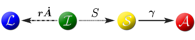
Figure 1: (Color online) Schematic depiction of the LISA model. An ignorant $\mathcal{I}$ can become a Luddite $\mathcal{L}$ with rate $r\dot{A}$ (in a mean-field setting); an ignorant can also become a susceptible $\mathcal{S}$ by contagion with rate proportional to the susceptible density. A susceptible spontaneously becomes an adopter at rate $\gamma$.

Our LISA model is a four-state system that consists of a population of $N$ individuals that can each be in the states of Luddite ($\mathcal{L}$), ignorant ($\mathcal{I}$), susceptible ($\mathcal{S}$), or adopter ($\mathcal{A}$). Ignorant agents may either be persuaded to become susceptible, and thence reach the adopter state, or they may become a Luddite and permanently oppose the spread of the innovation. Specifically, the elemental steps of our LISA model are the following (see Fig. 1):

1. Contagion-driven conversion: An ignorant agent becomes susceptible by interacting with another susceptible agent. That is, $\mathcal{I}+\mathcal{S}\to\mathcal{S}+\mathcal{S}$ with rate 1.

2. Spontaneous adoption: A susceptible agent spontaneously becomes an adopter, $\mathcal{S}\to\mathcal{A}$ with rate $\gamma$ .

3. Luddism: Ignorants may permanently reject the innovation and become Luddites, $\mathcal{I}\to\mathcal{L}$, with a rate proportional to the change in the density of adopters in its neighborhood.

The Luddism mechanism outlined above incorporates two aspects of negative behavior towards innovation. The first represents a fear of innovation or its consequences, as in the case of the historical Luddism movement, where the introduction of labor-saving machinery caused fear over job security Luddites_hist . The second is that of non-conformity; agents may oppose the innovation simply due to its rapid increase in popularity bandWagon . We model this feature by defining the rate at which the Luddite density increases to be proportional to the adoption rate, with constant of proportionality denoted by $r$, the Luddism parameter.

The multi-stage progression $\mathcal{I}\to\mathcal{S}\to\mathcal{A}$ may also be viewed as a type of social reinforcement mechanism in which adoption follows from a succession of prompts from neighbors Cth ; reinf . The equivalent 3-state model with only Luddites, ignorants and adopters creates a polarized community creates a polarized community where the ratio of adopters to Luddites is dependent only on the Luddism parameter, $r$. Other relevant models resistance have found that high levels of advertising can prompt a negative response to innovation which cannot be replicated with only three states. The combination of a multi-stage progression to adoption, together with the Luddite mechanism, arguably represents the simplest generalization of the Bass model that gives rise to non-trivial long-time state with incomplete adoption of an innovation.

III Mean-field descriptions

We first consider the LISA model in the mean-field limit, where agents are perfectly mixed. The densities of each type of agent are given by $(L,I,S,A)=(N_{\mathcal{L}},N_{\mathcal{I}},N_{\mathcal{S}},N_{\mathcal{A}})/N$, where $N_{X}$ is the number of agents of type $X\in\{\mathcal{L},\mathcal{I},\mathcal{S},\mathcal{A}\}$, and $N$ is the total number of agents. We consider the limit $N\to\infty$, so that all densities are continuous variables and all fluctuations are negligible. In this setting, the evolution of the agent densities is described by the rate equations:

$$\begin{split}\dot{L}&=r\dot{A}I\equiv(\alpha-1)SI,\\ \dot{I}&=-(1+\gamma r)SI\equiv-\alpha SI,\\ \dot{S}&=S(I-\gamma),\\ \dot{A}&=\gamma S,\end{split}$$ (1)

where the dot denotes the time derivative and we define $\alpha\equiv 1+\gamma r$. Since the total density is conserved, i.e., $L+I+S+A=1$, the sum of these rate equations equals zero. A natural initial condition is a population that consists of a small density of susceptible agents that initiate the dynamics, while all other agents are ignorant; that is, $I(0)=1-S(0)=I_{0}$ and $L(0)=A(0)=0$.

To solve these rate equations, it is useful to introduce the modified time variable $d\tau=S(t)\,dt$, which linearize the rate equations to

$$\begin{split}L^{\prime}&=(\alpha-1)I,\\ I^{\prime}&=-\alpha I,\\ S^{\prime}&=I-\gamma,\\ A^{\prime}&=\gamma,\end{split}$$ (2)

with solution

$$\begin{split}L&=\frac{\alpha-1}{\alpha}I_{0}(1-e^{-\alpha\tau}),\\ I&=I_{0}e^{-\alpha\tau},\\ S&=\frac{I_{0}}{\alpha}(1-e^{-\alpha\tau})+1-I_{0}-\gamma\tau,\\ A&=\gamma\tau.\end{split}$$ (3)

There are two basic regimes of behavior that are controlled by the adoption rate $\gamma$, as illustrated in Fig. 2:

1. Extensive adoption. When $\gamma<I_{0}$, the density of susceptibles $S$ varies non-monotonically in time and reaches a maximum value $S_{\rm inc}$ at an “inception” time $t_{\rm inc}$, after which $S$ decays to 0. This non-monotonicity leads to a sigmoidal curve for the adopter density, with $A$ increasing rapidly for $t\lesssim t_{\rm inc}$ and increasing very slowly for $t\gtrsim t_{\rm inc}$. The rescaled inception time $\tau_{\rm inc}$ is determined by the criterion $S^{\prime}=0$, or equivalently, $I(\tau_{\rm inc})=\gamma$. This gives

   $$\tau_{\rm inc}=\frac{1}{\alpha}\ln(I_{0}/\gamma)\,.$$ (4)

2. Sparse adoption. When $\gamma>I_{0}$, the susceptibles quickly become adopters, leaving behind a substantial static population of ignorants and a small fraction of adopters, as well as Luddites.

Numerical simulations of the LISA model on a large complete graph and numerical integration of the rate equations (1), illustrated in Fig. 2, give results that are virtually indistinguishable.

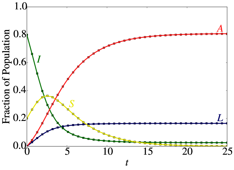
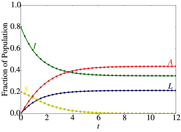
Figure 2: (Color online) Evolution of a realization of the LISA model on a complete graph of $10^{6}$ nodes with $I_{0}=0.8$ and Luddism parameter $r=0.9$. (a) $\gamma=0.3$ (extensive adoption) (b) $\gamma=1$ (sparse adoption). Evenly distributed samples of the stochastic simulation ($\Box$) are indistinguishable from the solution of Eq. (1) (solid line). The completion times for (a) and (b) are $60$ and $17$ respectively.

We can express the densities in terms of the physical time $t$ by inverting $d\tau=S(t)dt$ to give $t=\int_{0}^{\tau}d\tau^{\prime}/S(\tau^{\prime})$. Substituting $S(\tau)$ from the third of Eqs. (3) and taking the limits of low adoption, $\gamma\ll 1$ and $\alpha\approx 1$, we have 

$$t=\int_{0}^{\tau}\!\!\frac{d\tau^{\prime}}{1-I_{0}e^{-\tau^{\prime}}}\approx\tau+\ln\left[1-I_{0}e^{-\tau}\right]\,.$$ (5)

In particular, the physical inception time $t_{\rm inc}$ is,

$$t_{\rm inc}\approx\int_{0}^{\ln(I_{0}/\gamma)}\!\!\frac{d\tau^{\prime}}{1-I_{0}e^{-\tau^{\prime}}}\approx\ln\left[\frac{I_{0}}{(1-I_{0})\gamma}\right]$$ (6)

and therefore grows as $\ln(1/\gamma)$.

The stationary state is reached when all susceptibles disappear, so that no further reactions can occur. This gives the criterion $S(\tau_{\infty})=0$ which defines the value of $\tau_{\infty}$. By solving the third line of Eq. (3), we obtain

$$\tau_{\infty}=\frac{1}{\gamma}\!-\!\frac{I_{0}r}{\alpha}\!+\!\frac{1}{\alpha}W_{0}\left(-\frac{I_{0}}{\gamma}e^{I_{0}r-\alpha/\gamma}\right)\,,$$ (7)

where $W_{0}(z)$ is the principal branch of the Lambert function $W(z)$, which is defined as the solution of $z=We^{W}$. Here $\tau_{\infty}$ is a decreasing function of the adoption rate $\gamma$, with $\tau_{\infty}\sim 1/\gamma$ in the high and low adoption rate regimes.

We now determine the final densities by substituting $\tau_{\infty}$ into Eqs. (3). For small adoption rate ($\gamma\ll 1$), this gives

$$A_{\infty} =1\!-\!\mathcal{O}(\gamma),$$

$$I_{\infty} \to 0,$$

$$L_{\infty} \approx(\alpha-1)I_{0}=\mathcal{O}(\gamma).$$

Similarly, the densities at the inception time are obtained by substituting $\tau_{\rm inc}$ into Eqs. (3). This yields $A(\tau_{\rm inc})+S(\tau_{\rm inc})=1-[(\alpha-1)I_{0}+\gamma]/\alpha$. Since $(\alpha-1)I_{0}\sim{\cal O}(\gamma)$, when $\gamma\ll 1$ and $r$ is finite, here the stationary density of adopters approximately equals the sum of the adopter and susceptible densities at the inception time, $A_{\infty}\approx A(\tau_{\rm inc})+S(\tau_{\rm inc})$. Hence, in the low adoption rate regime (when $r$ is finite), we can infer the final level of adoption from the adopter and susceptible densities at the inception time, i.e., well before the stationary state.

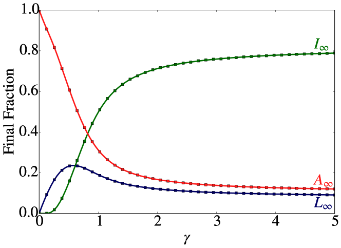
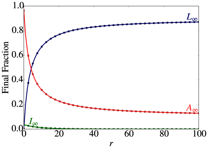
Figure 3: (Color online) Dependences of the final-state densities $L_{\infty},I_{\infty}$ and $A_{\infty}$ for a complete graph of $10^{4}$ nodes and $I_{0}=0.9$. In the top panel $r=0.9$ while $\gamma$ varies, whereas in the bottom panel $\gamma=0.3$ while $r$ varies. Simulations ($\Box$) in complete agreement with (3) with substitution (7) (solid line).

The dependence of the final densities for different parameter ranges is shown in Fig. 3. Again simulation results for the complete graph are indistinguishable from numerical integration of the rate equations. Interestingly, $L_{\infty}$ varies non-monotonically on $\gamma$ when the initial state consists mostly of ignorants and the fixed rate of Luddism $r$ is not too high, as in Fig. 3 (top). This non-monotonic dependence on $\gamma$ can be understood by noting that $dL_{\infty}/d\gamma\sim r(1-e^{-1/\gamma})>0$ for $\gamma\ll 1$ and $dL_{\infty}/d\gamma\sim-e^{-1/\gamma}/\gamma^{2}<0$ for $\gamma\gg 1$. We therefore expect that $L_{\infty}$ is peaked for an intermediate value of $\gamma$ on a range between the slow and quick adoption regimes. It is also worth noting that in the absence of Luddites, complete adoption is almost, but not completely achieved, since the final densities of adopters and ignorants are $A_{\infty}\approx 1-I_{\infty}$ and $I_{\infty}\approx e^{-1/\gamma}$, see Fig.3 (bottom).

To assess the role of finite-$N$ fluctuations on the dynamics, we simulate the LISA model on complete graphs of $N$ nodes using the Gillespie algorithm Gillespie . At long times we find that the densities of each species, $N_{X}/N$, fluctuates around the corresponding mean-field density, with a root-mean-square fluctuation of amplitude $\sim N^{-1/2}$, as expected from general properties of this class of reaction processes noise . We also find that the probability distribution of $N_{X}/N$ is a Gaussian of width of order $N^{-1/2}$ that is centered on the mean-field density. We also estimate the completion time $T_{C}$ for the system to reach its final state by the physical criterion that $S(t\!=\!T_{C})=1/N$. That is, completion is defined by the presence of a single susceptible remaining in the population reinf . By linearizing the rate equations (1) around $S_{\infty}=0$, the density of susceptibles asymptotically vanishes as $S(t)\sim e^{-(\gamma-I_{\infty})t}$. Hence, we estimate the mean completion time to be $T_{C}\approx(\ln~{}N)/(\gamma-I_{\infty})$. This prediction is confirmed by our simulations.

IV LISA model on random graphs and lattices

We now consider the behavior of the LISA model on Erdős-Rényi random graphs and one-dimensional lattices. We are particularly interested in uncovering dynamics that are characterized by genuine non mean-field effects.

A graph with $N$ nodes can be represented by its $N\times N$ adjacency matrix ${\bf A}=[A_{ij}]$, where $A_{ij}=1$ if nodes $i$ and $j$ are connected and $0$ otherwise. We implement the LISA model on such a graph using the Gillespie algorithm Gillespie . The propensity for a susceptible to become an adopter is $\gamma$, independent of the local environment. The propensity for an ignorant node $i$ to become susceptible if it has $s_{i}$ susceptible neighbors is $s_{i}/N$. The propensity of an ignorant node $i$ to become a Luddite is $r\gamma s_{i}/k_{i}$, where $k_{i}=\sum_{j}A_{ij}$ is the degree (number of neighbors) of node $i$, and $s_{i}/k_{i}$ is the fraction of nodes in the neighborhood of $i$ that are in the susceptible state. Thus the propensity of $i$ to become a Luddite is proportional to the sum of its susceptible neighbors’ propensities to adopt. This rate encodes node $i$’s local knowledge of the rate of adoption. These reaction rates approach those of the complete graph, described in Section III, as the average degree of the graph increases.

IV.1 Erdős-Rényi random graphs

We first study the LISA model on the class of Erdős-Rényi (ER) random graphs in which an edge between any two nodes occurs with a fixed probability $p$. This construction leads to a binomial degree distribution for the ER graph in which each node has, on average, $k=p(N-1)$ neighbors Newman2010 . Under the assumption of no correlations between the degrees of neighboring nodes, the adjacency matrix may be written as $A_{ij}\approx k_{i}k_{j}/(Nk)\approx k/N$. The LISA dynamics on ER graphs can now be approximately described by a natural generalization of the mean-field theory in which there are suitably defined reaction rates. In particular, if $S_{i}$ is the probability that a node $i$ is susceptible and $I_{j}$ is the probability that a node $j$ is ignorant, then the density of susceptibles $S$ evolves as

$$\dot{S_{i}}=S_{i}\Big{[}\sum_{j}(A_{ij}/N)I_{j}-\gamma\Big{]}\approx S\big{[}(k/N)I-\gamma\big{]},$$

since each susceptible interacts with $k$ of its $N$ neighbors on average. Thus on the ER graph there is a rescaling of the rate of the two-body contagion process $\mathcal{I}+\mathcal{S}\to\mathcal{S}+\mathcal{S}$, whereas the rates of the remaining one-body processes remain unaltered. Hence we obtain the effective rate equations

$$\begin{split}\dot{L}&=\gamma rSI\equiv\left(\beta-\frac{k}{N}\right)SI,\\ \dot{I}&=-\left(\gamma r+\frac{k}{N}\right)SI\equiv-\beta SI,\\ \dot{S}&=S\left(\frac{k}{N}~{}I-\gamma\right),\\ \dot{A}&=\gamma S,\\ \end{split}$$ (8)

where, for later convenience, we define $\beta\equiv\gamma r+(k/N)$.

As in the case of the mean-field dynamics, the above equations predict two regimes of behavior (see Fig. 4):

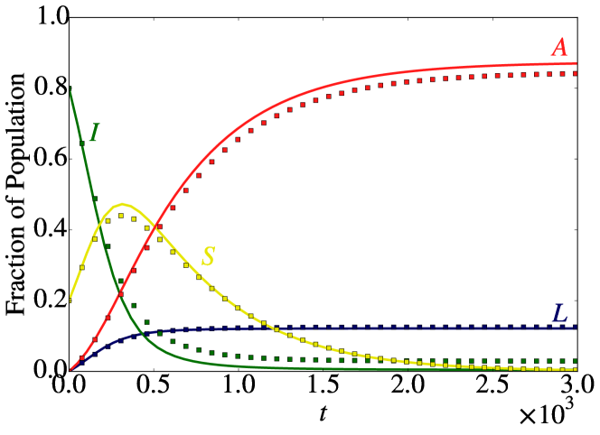
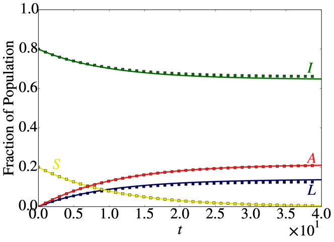
Figure 4: (Color online) The evolution, averaged over 100 realizations, of the LISA model on an ER graph with $N=10^{3}$ nodes, $k=10$, and $I_{0}=0.8$. (a) $\gamma=0.002$, such that $\gamma<(k/N)I_{0}$ and (b) $\gamma=0.1$ such that $\gamma>(k/N)I_{0}$. Shown are the evenly distributed samples of the stochastic simulation ($\Box$) and the solution of Eq. (8) (solid line). The Luddism parameter $r=0.9$.

1. Slow but extensive adoption ($\gamma<kI_{0}/N$). Here the density of $\mathcal{S}$’s peaks at a inception time $t_{\rm inc}\sim\ln(1/\gamma)$ before vanishing.

2. Rapid but sparse adoption ($\gamma>kI_{0}/N$). The density of $\mathcal{S}$’s vanishes quickly so that the density of adopters and Luddites quickly reach their steady-state values.

The simulation results presented in Fig. 4 indicate that the mean-field approximation (8) correctly captures the main qualitative features of the dynamics on large ER graphs. When $\gamma<kI_{0}/N$, the densities of $\mathcal{A}$ and $\mathcal{L}$ are characterized by a sigmoidal time dependence, whereas the density of $\mathcal{S}$ has a peak at the inception time $t_{\rm inc}$, with time evolution that is slower than on complete graphs, since each agent has now a finite neighborhood.

The stationary state can be determined by again noting that (8) becomes linear in terms of the variable $\tau=\int_{0}^{t}S(t^{\prime})dt^{\prime}$. Thus proceeding as in Section III, we find the steady state by the condition $S(\tau_{\infty})=0$. This yields

$$\begin{split}I_{\infty}&=I_{0}e^{-\beta\tau_{\infty}}\\ L_{\infty}&=\frac{\beta-k/N}{\beta}(I_{0}-I_{\infty})\\ A_{\infty}&=\gamma\tau_{\infty},\\ \end{split}$$ (9)

where now

$$\tau_{\infty} =\frac{k}{N\gamma\beta}+(1-I_{0})\frac{r}{\beta}$$

$$\hskip 36.135pt+\frac{1}{\beta}W_{0}\left(-\frac{kI_{0}}{N\gamma}e^{-(1-I_{0})r-k/(N\gamma)}\right)\,.$$ (10)

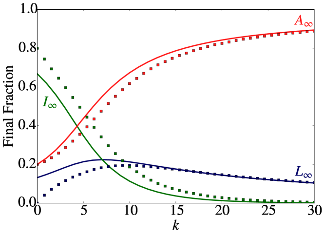
Figure 5: (Color online) Dependence of the final densities $L_{\infty},I_{\infty}$ and $A_{\infty}$ on the average degree for ER graphs with $N=10^{3}$ nodes. The simulation ($\Box$) represents an average over $40$ model realizations for $30$ randomly generated networks. Parameters are $\gamma=0.005,r=0.9$, and $I_{0}=0.9$. The mean-field predictions (9) (solid line) match the simulation for $k\gtrsim 20$ (see main text).

It is instructive to compare the predictions (9) with the results of stochastic simulations, and also compare with the equivalent results for the complete graph. Figure 5 shows simulation results for the stationary densities as a function of the mean degree. These results confirm that the mean-field predictions correctly capture the functional dependence of the steady state on the various parameters. However, the mean-field predictions (9) are quantitatively accurate only when $k/N$ is large. If $k/N\ll 1$, the neighborhood of each agent represents a small fraction of the entire network, and resulting large demographic fluctuations invalidate the assumptions underlying the derivation of (9). The dependence on $\gamma$ and $r$ are qualitatively similar to those observed on complete graphs.

The influence of demographic fluctuations can be heuristically assessed by viewing ER graphs of mean degree $k$ as a meta-population that consists of $N/k$ patches each comprising a well-mixed population of size $k$. According to this picture, when $N\gg k\gg 1$, the number of agents in each of the $N/k$ components fluctuates in a range of $k^{1/2}$ about its average value. Since these are independent fluctuations, the noise in the whole population should have an amplitude $\sim(N/k)^{1/2}\,k^{1/2}=N^{1/2}$, which leads to fluctuations in the densities of order $N^{-1/2}$. This prediction is confirmed by our simulations—we find that $N_{A}(\infty)/N$ has a Gaussian probability distribution around $A_{\infty}$ with a width that decays as $N^{-1/2}$. The same behavior is observed for $L_{\infty}$ and $I_{\infty}$ but not for $S_{\infty}$ as $S_{\infty}=0$ is a requirement for the completion of the dynamics.

The mean-field steady state predictions (9) are summarized in Fig. 6, where we plot the mean-field steady state predictions corresponding to each pair of steady state densities being equal. For example, the solid curve corresponds to parameter values for which $A_{\infty}=I_{\infty}$. This carves up the $(\gamma,r)$ parameter space into regions corresponding to different orderings of the steady state densities, labelled with Roman numerals in Fig. 6. We can use these orderings to interpret, from a marketing perspective, whether or not these would be considered successful campaigns. In this context, the most desirable outcome would be region (I), where adopters form the largest steady-state group and Luddites form the smallest. Whilst adopters also form the largest group in region (II), Luddites form the second largest group and so this region could be considered a controversial success — despite the majority adopting, a significant number of people have responded negatively. Conversely, regions (III) and (IV) could both be considered controversial failures because Luddites form the largest groups. Regions (V) and (VI) represent ineffective campaigns because ignorants form the largest steady state groups.

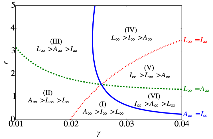
Figure 6: (Color online) The mean-field steady state predictions (9) over the parameter space $(\gamma,r)$ for $k/N=0.025$ and $I_{0}=0.9$. The contours $L_{\infty}=I_{\infty}$, $L_{\infty}=A_{\infty}$, and $I_{\infty}=A_{\infty}$ split the domain into six regions which characterize the innovation (see main text).

In summary, we have shown that the LISA dynamics on ER graphs can be accurately approximated by using mean-field assumptions, provided that the average degree is sufficiently high (see Fig. 5).

IV.2 One-dimensional lattices

Recent controlled experiments have shown that innovation may spread more efficiently on clustered graphs and lattices than on random networks C10 . To understand the effect of regular topology on the spread of an innovation, and where the mean-field approximation breaks down, we investigate the LISA dynamics on one-dimensional lattices.

The two regimes of behavior predicted by the mean-field description (8) on ER random graphs (see Section IV.1) also occur on one-dimensional lattices, despite the difference in topology. Specifically with $k=2$ we observe slow adoption for $\gamma<(2/N)I_{0}$ and fast adoption for $\gamma>(2/N)I_{0}$. From simulations, illustrated in Fig.7, we observe the following three regimes:

1. When $\gamma\ll 2I_{0}/N$, there is slow adoption as well as a time-scale separation. First, almost all $\mathcal{I}$’s are converted to $\mathcal{S}$’s 1D in a time of the order of $N^{2}$. When the lattice consists almost entirely of $\mathcal{S}$’s, these become adopters after a mean time of the order of $\gamma^{-1}$. As a consequence, when $\gamma\ll N^{-1}$ the size of the adopter domains grows abruptly after a time of order $\sim N^{2}+\gamma^{-1}$, when all ignorants have disappeared and the entire lattice is covered with adopters.

2. When $\gamma\sim 2I_{0}/N$, the domains of adopters grow initially nearly linearly in time, whereas the average size of ${\cal I}$ clusters remains approximately constant and of a comparable size to ${\cal A}$ domains.

3. When $\gamma\gg(2/N)I_{0}$, adoption occurs quickly and the final state is reached in a time of order ${\cal O}(1/\gamma)$. The final adopter density is limited by the formation of Luddites at the ends of ignorant domains which prevent further conversion within each domain.

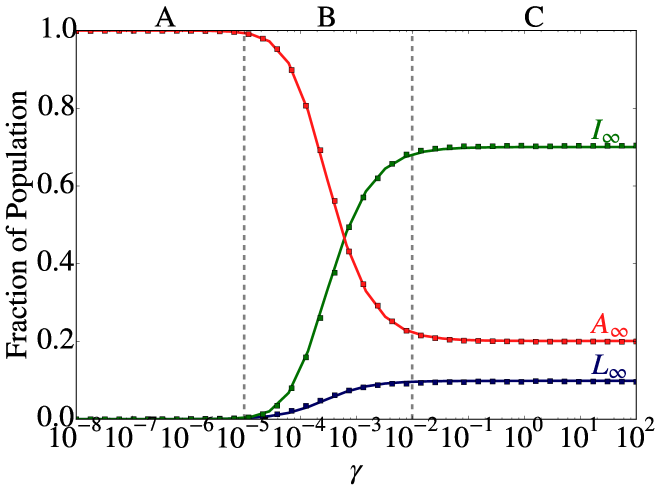
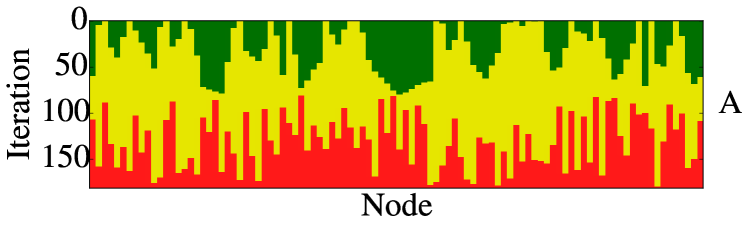
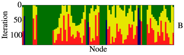
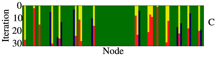
Figure 7: (Color online) Final simulated average proportions of adopters (red/gray $\Box$), ignorants (green/dark gray $\Box$) and Luddites (blue/black $\Box$) for varying values of $\gamma$, averaged over 100 simulations. Theoretical predictions using ignorant domain length (see Appendix A for details) are overlaid (solid line). Parameters are $N=1000$, $r=0.5$. Initially ignorants and susceptibles are randomly distributed, with densities $I_{0}=0.8$ and $S_{0}=0.2$. The three regimes discussed in the text are separated by dashed lines corresponding to regions where $(2/N)I_{0}\ll\gamma$ and $(2/N)I_{0}\gg\gamma$. Typical realizations of the model for $N=100$ in each of the three regimes are given (bottom). On the vertical axis the iteration corresponds to a single step of the Gillespie algorithm, with one reaction taking place per iteration.

While the mean-field approximation (8) predicts the correct regimes of behavior, the agreement is only qualitative. In Fig. 8 we compare typical simulations of the LISA model on a one-dimensional lattice with the mean-field predictions of (8) for the case of $k=2$.

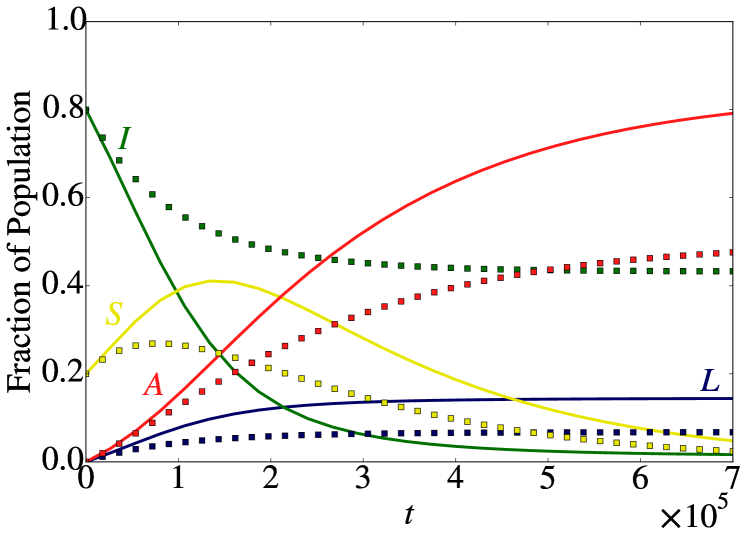
Figure 8: (Color online) Time dependence of the densities in each state for a one-dimensional lattice of size $N=10^{5}$ averaged over 100 realizations. The corresponding mean-field predictions from Eq. (8) with $k=2$ (solid line) deviate dramatically from the simulation samples ($\Box$). The parameters are $\gamma=0.005,r=0.9$, and $I_{0}=0.8$.

The simulations and mean-field predictions (8) systematically deviate; the latter always overestimates the final density of adopters and underestimates the final density of ignorants. This can be attributed to the topological constraints on one-dimensional lattices. Initially the lattice comprises of contiguous domains of ignorants that are separated by domains of one or more neighboring susceptibles. Since ignorants can only become susceptible if a neighbor is susceptible, domains of ignorants shrink at their interfaces with susceptibles. Crucially, the evolution of an ignorant-susceptible interface ceases if either the susceptible at the interface adopts or the ignorant at the interface becomes a Luddite. Thus in one dimension both Luddites and adopters act as barriers to the spread of adoption, an effect that is not captured by the mean-field description.

Since domains of ignorants decrease in size and evolve independently, we can determine analytically the expected final length of ignorant domains $\langle x\rangle$ and hence the final fractions of each type of agent. The details of these calculations are given in Appendix A. Briefly, we first determine the probability $P_{n}(m)$ that a domain of ignorants of initial length $n$ shrinks by $m$. We then use $P_{n}(m)$ to calculate the expected final length of ignorant domains $\langle x\rangle$ and the final fraction of ignorants. Since Luddites only form at the boundaries of ignorant domains, we are able also to determine the expected final fraction of Luddites and hence, using the conservation relation $L+I+S+A=1$, the final fraction of adopters. The resulting final fractions of each type of agent are plotted in Fig. 7 and agree extremely well with the corresponding numerical simulations. In principle, this method allows us to derive explicit formulas for the final fractions of each agent; however, in practice these formulas prove cumbersome.

V Discussion & conclusion

Innovations are often accompanied by societal debates and controversies that may lead to divisions between adopters of an innovation and those who permanently reject that innovation. Consequently, innovations are rarely adopted by the whole population, as various examples, ranging from technology to medicine, demonstrate. Classical models of innovation diffusion, such as that proposed by Bass, assume a “pro-innovation bias” and predict the complete adoption of innovations.

Motivated by these considerations we have introduced a multi-stage generalization of the Bass model, the LISA model, that does not unavoidably lead to complete adoption. The main new feature of our model is the introduction of Luddites that permanently oppose the spread of innovation in their neighborhood. In the LISA model, ignorant individuals can successively become susceptibles and then adopters, or turn to Luddism in response to a high rate of adoption and permanently reject the innovation.

We carried out a detailed analysis of the properties of the LISA model on complete graphs and Erdős-Rényi random graphs, as well as on one-dimensional lattices. In particular, we focused on the steady states and completion time (time to reach stationarity). We showed that significant insights can be gained from a simple mean-field analysis that aptly captures the qualitative aspects of the two basic regimes of the LISA dynamics. When the rate of adoption is low, the population slowly converges to a final state that consists of a high concentration of adopters. In the converse case, the stationary state is reached much more quickly, but the final fraction of adopters is much lower and is severely limited by the significant densities of Luddites and ignorants.

Since most models of innovation diffusion are formulated at mean-field level, an important aspect of this work has also been to reveal the limitations of the mean-field approximation. In particular, for Erdős-Rényi random graphs with low mean degree and one-dimensional lattices, the mean-field approximation proves inaccurate. This is due to the formation of Luddites which isolate domains of ignorants from the innovation, an effect particularly apparently in one dimension. It would be worthwhile to investigate the LISA model on modular networks, where Luddism has the potential to block the spread of innovation to entire communities. In addition to the work described in this paper, we also found that the mean-field approximation proves better on two-dimensional lattices than on one-dimensional lattices.

In summary, the LISA model is a simple, but non-trivial, innovation diffusion model that accounts for the possibility that the promotion of an innovation may be tempered by the alienation of some individuals. These in turn affect the spread of the innovation. Interestingly, our model outlines two possible marketing scenarios: If one is interested in reaching a high level of adoption then this can only be achieved over long time scales, since the rate of adoption must be low. However, if the priority is to attain a finite level of adoption as quickly as possible regardless of the alienation that this may cause, then a high rate of adoption is preferable.

VI Acknowledgements

This work is supported by an EPSRC Industrial Case Studentship Grant No. EP/L50550X/1. SR is supported in part by NSF Grant No. DMR-1205797. Partial funding from Bloom Agency in Leeds U.K. is also gratefully acknowledged.

Appendix A Analysis of one-dimensional dynamics

In this appendix we describe the calculation of the final fractions of each type of agent on one-dimensional lattices. These results are compared with simulations in Fig. 7 of Section IV.2.

A.1 Analysis of ignorant domains

Initially, the nodes on the one-dimensional lattice are either ignorant, with probability $I_{0}$, or susceptible, with probability $S_{0}=1-I_{0}$. Thus the initial configuration consists of connected domains of ignorant nodes bordered by susceptibles. Moreover, since ignorants can only become susceptible if a neighbor is susceptible, domains of ignorants only evolve at their ignorant-susceptible interfaces. We will refer to these as “active interfaces”. At an active interface one of three events can occur:

• The ignorant node becomes susceptible, thus reducing the domain length by one, with probability

  $$p_{S}=\frac{1/N}{1/N+r\gamma/2+\gamma}.$$

• The ignorant node becomes a Luddite, thus reducing the length of the domain by one and causing the interface to become inactive, with probability

  $$p_{L}=\frac{r\gamma/2}{1/N+r\gamma/2+\gamma}.$$

• The susceptible node becomes an adopter, thereby terminating the interface evolution, with probability

  $$p_{A}=\frac{\gamma}{1/N+r\gamma/2+\gamma}.$$

For an isolated ignorant node with two susceptible neighbors, these probabilities respectively become

$$\hat{p}_{S}= \frac{2/N}{2/N+r\gamma+\gamma},$$

$$\hat{p}_{L}= \frac{r\gamma}{2/N+r\gamma+\gamma},$$

$$\hat{p}_{A}= \frac{\gamma}{2/N+r\gamma+\gamma}.$$

Let $Q_{n}(m)$ be the probability that a domain of ignorants of initial length $n$ with a single ignorant-susceptible interface has a final length $n-m$, with $0\leq m\leq n$. We can determine $Q_{n}(m)$ as follows: If the final length of ignorants is $n-m$, with $0<m<n$, then either $m$ ignorant nodes must become susceptible before a susceptible node at the interface adopts, or $m-1$ ignorant nodes must become susceptible before an ignorant node at the interface becomes a Luddite. These events occur with probabilities $p_{A}p_{S}^{m}$ and $p_{L}p_{S}^{m-1}$ respectively. Using similar reasoning for the cases $m=0$ and $m=n$, we thus find

$$Q_{n}(m)=\left\{\begin{array}[]{crl}p_{A}&\text{if}&m=0\\ p_{A}p_{S}^{m}+p_{L}p_{S}^{m-1}&\text{if}&0<m<n\\ p_{S}^{n}+p_{L}p_{S}^{n-1}&\text{if}&m=n\end{array}\right..$$ (11)

By summing over $m$, it can be shown that $Q_{n}(m)$ is normalized.

We now consider the case where a connected region of $n$ ignorant nodes initially has two ignorant-susceptible interfaces. The probability $P_{n}(m)$ that a region of ignorants of initial length $n$ with two active interfaces has final length $n-m$ is given by the recursion relation

$$P_{n}(m) =Q_{n}(m)p_{A}+Q_{n-1}(m-1)p_{L}$$

$$\hskip 28.45274pt+P_{n-1}(m-1)p_{S},$$ (12)

where the terms $Q_{n}(m)$ are given by (11). Equation (12) captures the three possible events that can occur at the interface. If a susceptible node at the interface adopts, which occurs with probability $p_{A}$, then the region of ignorants only has one remaining active interface left and there will be $n-m$ remaining ignorants with probability $Q_{n}(m)$, as given in (11). If an ignorant node at the interface becomes a Luddite, which occurs with probability $p_{L}$, then again the region of ignorants will only have one active interface. Since there will be one ignorant less the probability there will be $n-m$ remaining ignorants is $Q_{n-1}(m-1)$. Finally, if an ignorant node at the boundary becomes susceptible, which occurs with probability $p_{S}$, then the probability that there are $n-m$ ignorants remaining is the same as if we had started with $n-1$ ignorant nodes, i.e. $P_{n-1}(m-1)$.

To solve the recursion relation (12) we need $P_{n}(0)$ and $P_{1}(1)$. The probability that a region of ignorants of initial length $n$ remains of length $n$ is given by

$$P_{n}(0)=\left\{\begin{array}[]{crl}p_{A}\hat{p}_{A}&\text{if}&n=1\\ p_{A}^{2}&\text{if}&n>1\end{array}\right..$$

Also, the probability that a single ignorant node that initially has two susceptible neighbors becomes a susceptible or Luddite is given by

$$P_{1}(1)=\hat{p}_{A}(p_{L}+p_{S})+\hat{p}_{L}+\hat{p}_{S}.$$

Thus the solution to the recursion relation (12) for $0<m<n-1$ is given by

$$P_{n}(m) =(m+1)p_{A}^{2}p_{S}^{m}+2mp_{A}p_{L}p_{S}^{m-1}$$

$$+(m-1)p_{L}^{2}p_{S}^{m-2}.$$

For $m=n-1$ we have

$$P_{n}(n-1) =p_{A}\left[\hat{p}_{A}+(n-1)p_{A}\right]p_{S}^{n-1}$$

$$+2(n-1)p_{A}p_{L}p_{S}^{n-2}+(n-2)p_{L}^{2}p_{S}^{n-3},$$

and for $m=n$ we have

$$P_{n}(n) =\left[\hat{p}_{A}(p_{L}+p_{S})+\hat{p}_{L}+\hat{p}_{S}\right]p_{S}^{n-1}$$

$$+(n-1)\left(p_{A}p_{S}^{n}+2p_{L}p_{S}^{n-1}+p_{L}^{2}p_{S}^{n-2}\right).$$

Again it is possible to check, by summing (12) over $m$ and solving the resulting recursion relation, that $P_{n}(m)$ is normalized.

We can use $P_{n}(m)$ to calculate the expected final length of ignorant domains $\langle x\rangle$. First note that since $I_{0}$ is the initial probability of being ignorant, the probability that a domain of ignorants initially has length $n>0$ is given by $p_{0}(n)=I_{0}^{n-1}S_{0}$ for large $N$. Thus we find that

$$\langle x\rangle=\sum_{n=0}^{N}np_{0}(n)-\sum_{n=0}^{N}p_{0}(n)\sum_{l=0}^{n}lP_{n}(l).$$

In principle, we may use the above to obtain an explicit expression for $\langle x\rangle$. In practice, however, we use the solutions to (12) to calculate $\langle x\rangle$ numerically.

A.2 Calculation of population densities

Initially, the mean number of ignorants is given by $I_{0}N$ and so dividing by the mean length of ignorant domains, $1/(1-I_{0})$, yields the expected number of ignorant domains, $(1-I_{0})I_{0}N$. Thus the final density of ignorants is

$$I_{\infty}=(1-I_{0})I_{0}\langle x\rangle.$$

The probability that an ignorant domain survives is

$$q=1-\sum_{n=0}^{\infty}p_{0}(n)P_{n}(n).$$

Surviving ignorant domains have two interfaces, which are either ignorant-adopter or ignorant-Luddite, with probabilities $p_{A}/(p_{L}+p_{A})$ and $p_{L}/(p_{L}+p_{A})$, respectively. Thus the expected number of Luddites at the interfaces of non-vanishing ignorant domains is given by

$$\eta_{+}=\frac{2p_{L}}{p_{L}+p_{A}}q(1-I_{0})I_{0}N.$$ (13)

It is also possible for Luddites to arise when a domain vanishes. By identifying the terms in $P_{n}(n)$ that result in Luddites, it is possible to determine that the expected number of Luddites that arise when a domain of initial size $n>1$ vanishes is given by

$$l_{n}=\left(\hat{p}_{A}p_{L}+\hat{p}_{L}\right)p_{S}^{n-1}+(n-1)\left(2p_{L}p_{S}^{n-1}+p_{L}^{2}p_{S}^{n-2}\right)$$

and $l_{1}=\hat{p}_{A}p_{L}+\hat{p}_{L}$. Thus the expected number of Luddites that arise from domains of ignorants that vanish is

$$\eta_{0}=(1-I_{0})I_{0}N\sum_{n=0}^{\infty}p_{0}(n)l_{n}.$$ (14)

Summing Eqs. (13) and (14) and dividing by $N$ we arrive at the final density of Luddites

$$L_{\infty}=I_{0}(1-I_{0})\left(\frac{2p_{L}}{p_{L}+p_{A}}q+\sum_{n=0}^{\infty}p_{0}(n)l_{n}\right).$$

Since the dynamics cease when $S=0$, the number of adopters can be found using the conservation law $A_{\infty}=1-L_{\infty}-I_{\infty}$.

References

- (1) E. M. Rogers, Diffusion of Innovations (Free Press, New York, 2003).
- (2) D. L. Kincaid, J. of Health Comm. 9, 37 (2004).
- (3) B. Ryan and N. Gross, Rural Sociology 8, 15 (1943).
- (4) J. Coleman, E. Katz, and H. Menzel, Sociometry 20, 253 (1957).
- (5) L. A. Fourt and J. W. Woodlock, Journal of Marketing 25 31 (1960); E. Mansfield, Econometrica 29, 741 (1961).
- (6) F. M. Bass, Management Science 15, 215 (1969).
- (7) F. M. Bass, J. Business 53, S51 (1980).
- (8) V. Mahajan, E. Muller, and F. M. Bass, Journal of Marketing 54, 1 (1990).
- (9) F. M. Bass, Management Science 50, 1833 (2004).
- (10) W. J. Hopp, Management Science 50, 1763 (2004).
- (11) M. G. Dekimpe, P. M. Parker and M. Sarvary, Technol. Forecast. Soc. Change 57, 105 (1998); S. Sundqvista, L. Franka and K. Puumalainen, J. Bus. Res. 58, 107 (2005); C. Michalakelis, D. Varoutas and T. Sphicopoulos, Telecommun. Policy 32, 234 (2008): J. Lim, C. Nam, S. Kim, H. Rhee, E. Lee and H. Lee, Telecommun. Policy 36, 858 (2012); J. L. Toole, M. Cha, and M. C. Gonzalez, PLoS One 7, e29528 (2012).
- (12) E. Kiesling et al., CEJOR 20, 183 (2012).
- (13) H. Peyton Young, American Economic Review, 99, 1899 (2009).
- (14) F. Sultan, J. U. Farley, D. R. Lehmann DR, Journal of Marketing 27 70 (1990).
- (15) R. M. Heeler, T. P. Hustad, Management Science 26, 1007 (1980); C. Van den Bulte, G. L. Lilien, Marketing Science 16, 338 (1997); R. Kohli, D. R. Lehmann, J. Pae, J. Product Innovation Management 16, 134 (1999).
- (16) M Hohnisch, S. Pittnauer, and D. Stauffer, Industrial and Corporate Change 17, 1001 (2008).
- (17) D. Centola, Science 329, 1194 (2010).
- (18) D. Centola, R. Wilker, and M. W. Macy, Am. J. Sociol. 110, 1009 (2005); D. Centola, V. M Eguiluz, and M. W. Macy, Physica A 374, 449 (2007).
- (19) P. S. Dodds and D. J. Watts, Phys. Rev. Lett. 92, 218701 (2004); H. P. Young, Amer. Econ. Rev. 99, 1899 (2009); P. L. Krapivsky, S. Redner, and D. Volovik, J. Stat. Mech. P12003 (2011).
- (20) J. Goldenberg, B. Libai, S. Solomon, N. Jan N, and D. Stauffer, Physica A 284, 335 (2000); D. Strang D and M. W. Macy, American Journal of Sociology 107, 147 (2001).
- (21) P. S. Tolbert and L. G. Zucker, Admin. Science Quarterly 28, 22 (1983); E. Abrahamson and L. Rosenkopf, Acad. Management Review 18, 487 (1993); L. Rosenkopf and E. Abrahamson, Comp. and Math. Organization Theory 5, 361 (1999).
- (22) http://www.pewinternet.org/data-trend/mobile/device-ownership/
- (23) http://interphone.iarc.fr/UICCReportFinal03102011.pdf
- (24) R. M. Wolfe and L. K. Sharp, BMJ 325, 430 (2002).
- (25) http://www.hscic.gov.uk/catalogue/PUB14949/nhs-immu-stat-eng-2013-14-rep.pdf
- (26) D. J. Watts and P. S. Dodds, J Cons Res 34, 441 (2007); G. Kocsis and F. Kun, J. Stat. Mech. P10014 (2008); M. Lin, N. Li, Physica A 389, 473 (2010); G. Pegoretti, F. Rentocchini, G. V. Marzetti, J. Econ. Interact. Coord. 7, 145 (2012); N. J. McCullen, A. M. Rucklidge, C. S. E. Bale, T. J. Foxon, and W. F. Gale, SIAM J. Applied Dynamical Systems 12, 515 (2013); S. Melnik, J. A. Ward, J. P. Gleeson, M. A. Porter, Chaos, 23, 013124 (2013); K. Sznajd-Weron, J. Szwabinski, R. Weron, T. Weron, J.Stat.Mech. (2014) P03007; P. Przybyla, K. Sznajd-Weron, R. Weron, Advances in Complex Systems 17 (2014) 1450004
- (27) S. Moldovan and J. Goldenberg, Technological Forecasting & Social Change 71 (2004) 425–442.
- (28) http://www.nationalarchives.gov.uk/education/politics/g3/
- (29) D. T. Gillespie, J. Comput. Phys. 22, 403 (1976).
- (30) M. Newman, Networks: An Introduction (Oxford University Press, Oxford, 2010); M. O. Jackson, Social and Economic Networks (Princeton University Press, Princeton, 2010).
- (31) N. G. Van Kampen, Stochastic Processes in Physics and Chemistry (Elsevier, 2007); C. Gardiner, Stochastic Methods (Springer, 2010).
- (32) Nonequilibrium Statistical Mechanics in One Dimension, edited by V. Privman (Cambridge University Press, New York, 1997); S. Redner, A Guide to First-Passage Processes (Cambridge University Press, New York, 2001); P. L. Krapivsky, S. Redner and E. Ben-Naim, A kinetic view of statistical physics (Cambridge University Press, New York, 2010).