Top Quark Pair Production beyond NNLO

Abstract

We construct an approximate expression for the total cross section for the production of a heavy quark-antiquark pair in hadronic collisions at next-to-next-to-next-to-leading order (N³LO) in $\alpha_{s}$. We use a technique which exploits the analyticity of the Mellin space cross section, and the information on its singularity structure coming from large $N$ (soft gluon, Sudakov) and small $N$ (high energy, BFKL) all order resummations, previously introduced and used in the case of Higgs production. We validate our method by comparing to available exact results up to NNLO. We find that N³LO corrections increase the predicted top pair cross section at the LHC by about 4% over the NNLO.

1 Introduction

The lack of discovery of any new physics signal so far has made of the Large Hadron Collider (LHC) even more a precision machine than it ever was. Because the LHC is a hadron collider, the largest uncertainties are related to nucleon structure, i.e. parton distributions, and higher order QCD corrections. This has consequently led to enormous progress in the computation of higher order corrections to QCD processes in the last several years, recently leading to the publication of first N³LO results for a hadron collider process Anastasiou:2015ema .

In Ref. Ball:2013bra some of us have proposed a general methodology for the determination of approximate expressions for higher-order corrections to QCD processes. The basic idea is that QCD corrections to many important hard processes are known to all orders in the strong coupling in two opposite limits: the high energy limit, in which the available center-of-mass energy is much greater than the invariant mass of the final state, and the soft limit, in which the invariant mass is close to threshold. By performing a Mellin transform, this knowledge can be turned into information on the singularities of the hard (partonic) Mellin-space cross section to any given finite order, viewed as an analytic function of the Mellin complex variable: the soft limit determines the singularity at infinity, and the high-energy limit determines the rightmost pole on the real axis. It is then possible to reconstruct an approximate form of the function by exploiting this knowledge: indeed, knowledge of all the singularities would determine the function completely.

The case of Higgs production, to which the methodology of Ref. Ball:2013bra was first applied Ball:2013bra ; Bonvini:2014jma ; Bonvini:2014joa , is particularly simple in many respects: the leading-order process has fixed kinematics (only one scalar colorless particle in the final state), and the total cross section is known Kramer:1996iq to be dominated by its threshold limit. The validation of the methodology which comes from checking that it provides a good approximation to known results in the case of Higgs is thus not necessarily the most compelling.

In this paper we turn our attention to heavy quark production: a process which is rather more complicated in terms of kinematics and color structure, with the goal of performing a more stringent test of our methodology. Next-to-leading (NLO) QCD corrections to this process were computed long ago Nason:1987xz ; Mangano:1991jk , though fully analytic expressions only became available much more recently Czakon:2008ii , and were a first necessary step towards the full determination of the NNLO result which was very recently achieved Baernreuther:2012ny ; Czakon:2012zr ; Czakon:2012pz ; Czakon:2013goa . These results revealed that the physical-space partonic cross section has a particularly complex singularity structure, which raises the question of how this relates to the Mellin-space singularities which are used for the approximation of Ref. Ball:2013bra , and also, that existing attempts at an approximate NNLO determination Moch:2012mk were rather off the mark.

Here, we will present an approximate determination of the N³LO QCD corrections to the total cross section for heavy quark production. In Section 2 we will review the singularity structure of the heavy quark production partonic cross section both in physical and in Mellin space. Specifically, we will discuss the relationship between the total cross section and the invariant mass distribution, to which the methods of Ref. Ball:2013bra apply, and show that the peculiar singularity structure of the physical-space cross section leads nevertheless to the standard Mellin-space singularities. The rest of our treatment closely follows that of Higgs production: in Sects. 3 and 4 respectively we present the derivation of the soft and high-energy singularities from the respective resummations. They are combined in Section 5 where we present our final result: first, we compare the approximation obtained through our procedure to the known exact result up to NNLO, and then we present our final approximate N³LO both at the parton and the hadron level.

2 Analytic structure of the partonic cross section

The analytic structure of the cross section for the production of a heavy quark pair potentially differs from that for Higgs production discussed in Ref. Ball:2013bra for two different reasons, thereby potentially hampering, or requiring some adaptation of the methods used in that reference. First, the known Czakon:2008ii fact that the partonic cross section for heavy quark production already at NLO has unphysical singularities in the complex plane of its kinematic variables may suggest that the singularity structure of its Mellin transform also does not follow the general pattern discussed in Ref. Ball:2013bra . Second, as we shall see in more detail below, the analytic structure discussed in Ref. Ball:2013bra is generic for partonic differential cross sections, while the case we are presently considering is that of a total cross section. We will see that the first issue is of no concern, while the second requires a careful discussion of the relation of the total heavy quark production cross section to the corresponding invariant mass distribution.

We will address the two issues in turn, after a quick review of standard notation and general results.

2.1 Notation and general results

The total cross section for the production of a heavy quark-antiquark pair can be written in factorized form as

$$\sigma(m^{2},\rho_{h})=\rho_{h}\sum_{ij}\int_{\rho_{h}}^{1}\frac{d\rho}{\rho}\,\mathscr{L}_{ij}\left(\frac{\rho_{h}}{\rho},\mu_{\rm\scriptscriptstyle\rm F}^{2}\right)\frac{1}{\rho}\hat{\sigma}_{ij}\left(m^{2},\rho,\alpha_{s}(\mu_{\rm\scriptscriptstyle\rm R}^{2}),\frac{m^{2}}{\mu_{\rm\scriptscriptstyle\rm F}^{2}},\frac{m^{2}}{\mu_{\rm\scriptscriptstyle\rm R}^{2}}\right)$$ (2.1)

where $\rho_{h}=4m^{2}/s$, $s$ is the hadronic center of mass energy, $\mathscr{L}_{ij}(\rho,\mu_{\rm\scriptscriptstyle\rm F}^{2})$ are parton luminosities, $m$ is the mass of the heavy quark, $\mu_{\rm\scriptscriptstyle\rm F},\mu_{\rm\scriptscriptstyle\rm R}$ are factorization and renormalization scales, and the scaling variable is $\rho=4m^{2}/\hat{s}$, with $\hat{s}$ the partonic center of mass energy. To simplify notations, in the following we will not indicate explicitly the dependence of parton luminosities on the factorization scale $\mu_{\rm\scriptscriptstyle\rm F}$ and that of the partonic cross section on the strong coupling and on $\mu_{\rm\scriptscriptstyle\rm F},\mu_{\rm\scriptscriptstyle\rm R}$.

The partonic cross sections $\hat{\sigma}_{ij}$ admit a perturbative expansion in powers of the QCD coupling:

$$\hat{\sigma}_{ij}(m^{2},\rho)=\frac{\alpha_{s}^{2}}{m^{2}}\left[\hat{\sigma}^{\left(0\right)}_{ij}(\rho)+\alpha_{s}\hat{\sigma}^{(1)}_{ij}(\rho)+\alpha_{s}^{2}\hat{\sigma}^{(2)}_{ij}(\rho)+\alpha_{s}^{3}\hat{\sigma}^{(3)}_{ij}(\rho)+\mathcal{O}(\alpha_{s}^{4})\right],$$ (2.2)

where, thanks to the $m^{-2}$ prefactor, the coefficients $\hat{\sigma}^{(k)}_{ij}(\rho)$ are dimensionless. Eq. (2.1) is in the form of a convolution product, so its Mellin transform

$$\sigma(m^{2},N)=\int_{0}^{1}d\rho_{h}\,\rho_{h}^{N-2}\sigma(m^{2},\rho_{h})$$ (2.3)

factorizes in terms of the Mellin space luminosity and partonic cross section function, defined respectively as

$$\mathscr{L}(N) =\int_{0}^{1}d\rho\,\rho^{N-1}\mathscr{L}(\rho)$$ (2.4)

$$\hat{\sigma}_{ij}(m^{2},N) =\int_{0}^{1}d\rho\,\rho^{N-2}\hat{\sigma}_{ij}(m^{2},\rho),$$ (2.5)

according to

$$\sigma(m^{2},N)=\sum_{ij}\mathscr{L}_{ij}(N)\hat{\sigma}_{ij}(m^{2},N).$$ (2.6)

If the Mellin transform integral has a finite convergence abscissa, the $N$-space partonic cross section is an analytic function of the complex variable $N$, defined by the integral representation Eq. (2.5) to the right of the convergence abscissa, and by analytic continuation elsewhere. Therefore, it is fully determined by the knowledge of its singularities.

In this paper, we will concentrate on the $gg$ partonic channel, which is the most relevant (in the $\overline{\rm MS}$ scheme) at LHC energies, while we leave the study of other parton subprocesses for future work. For this reason in the following we will drop the parton indices $ij$, with the understanding that $i=j=g$ in all parton luminosities and partonic cross sections.

The singularity structure of a generic differential partonic cross section is relatively simple. The singularity at infinity is determined by soft gluon radiation, which leads to a growth of the cross section with increasingly high powers of $\ln N$ at higher perturbative orders. For finite $N$, singularities away from the real axis are not allowed, as they would have to come in pairs and would thus lead to oscillatory behaviour of the cross section at high energy. From Regge theory one expects that the rightmost singularity on the real axis is a multiple pole located at $N=1$ Lipatov:polo , with further multiple poles along the real axis at $N=0,-1,-2,\dots$. This expectation is confirmed by explicit fixed-order calculations.

While knowledge of the residues of all poles is required in order to fully determine the function $\hat{\sigma}(m^{2},N)$, its behaviour in the region $1<\mathrm{Re}\>N<\infty$ is mostly controlled by the rightmost pole at $N=1$, with poles further to the left having an increasingly small impact. Using the saddle point approximation one can show that the hadronic cross section is mostly determined by the behaviour of the partonic cross section $\hat{\sigma}(m^{2},N)$ in the vicinity of a single (saddle) value of $N$ on the real axis, to the right of the rightmost singularity Bonvini:2012an ; Ball:2013bra (see also Sect. 5.1). In Ref. Ball:2013bra it was suggested that knowledge of the rightmost singularity on the real axis and of the singularity at infinity is sufficient to determine the partonic cross section in the region where the saddle-point is located with reasonable accuracy.

As mentioned in the introduction, however, in the specific case of heavy quark production, we encounter two difficulties. The first, is related to the fact that the physical momentum-space coefficient function has unphysical singularities. The second is due to the fact that the partonic cross sections $\hat{\sigma}_{ij}(m^{2},N)$ Eq. (2.6) vanish as $N\to\infty$, rather than growing logarithmically.

We will address both issues in turn. The first issue turns out to be of no concern: the analytic structure in Mellin space is unaffected by the unphysical momentum-space singularities. The second issue instead is due to the fact that the reason why the partonic cross sections discussed in Ref. Ball:2013bra grow as $N\to\infty$ is that they are distributions, rather than ordinary functions: indeed, elementary properties of Laplace transforms imply that the Mellin transform of an ordinary function, if it exists, must vanish as $N\to\infty$. Now, the integral of a distribution is an ordinary function, so it is clear that the behaviour of Ref. Ball:2013bra can only hold for partonic cross sections which are sufficiently differential. As we shall see below, it is the invariant-mass distribution which behaves at large $N$ in the way discussed in Ref. Ball:2013bra . However, by exploiting the relation between total cross section and invariant-mass distribution, it is possible to relate their respective large-$N$ behaviors, and define a coefficient function whose singularity structure follows the general pattern discussed above.

2.2 Unphysical singularities in momentum space

The perturbative coefficients $\hat{\sigma}_{ij}^{(k)}(\rho)$ display a class of spurious singularities in the complex $\rho$ plane outside the physical region $0<\rho\leq 1$. However, after Mellin transformation, even in the presence of such spurious singularities in $\rho$ space, the result has the expected analytic structure, as we now show.

As an example, we present the case of NLO corrections of top pair production in the $gg$ channel. In Ref. Czakon:2008ii , the complete analytic form of $\hat{\sigma}^{\left(1\right)}_{gg}\left(\rho\right)$ is computed, and it contains, in addition to the usual (physical) singularities in $\rho=1$ and $\rho=0$, four further singularities (branch points) located at $\rho=-4$, $\rho=4$, $\rho=-1$, $\rho=-\frac{1}{4}$ (see in particular the functions $F_{i}(\rho)$, $i=1,\ldots,4$ of section $4$ and the discussion of section $5$ of Ref. Czakon:2008ii ). For simplicity we focus our attention only on the first spurious singularity; similar considerations hold for all the others.

The function

$$F_{2}\left(\rho\right) =\int_{x(\rho)}^{1}dz\,f_{2}(z)$$ (2.7)

$$f_{2}(z) =-\frac{\left(2z+3\right)\left(12\ln z\ln\frac{1+z}{\sqrt{z}}+3\ln^{2}z+12\mathrm{Li}_{2}\left(-z\right)+\pi^{2}\right)}{4\left(z^{2}+3z+1\right)},$$ (2.8)

$$x(\rho) =\frac{1-\sqrt{1-\rho}}{1+\sqrt{1-\rho}}$$ (2.9)

has a logarithmic branch cut starting at $\rho=-4$, because the integrand has a simple pole in

$$z=\frac{\sqrt{5}-3}{2}=x(-4).$$ (2.10)

However, the Mellin transform is

$$F_{2}(N)=\int_{0}^{1}d\rho\,\rho^{N-2}\int_{x(\rho)}^{1}dz\,f_{2}(z)=\int_{0}^{1}dz\,f_{2}\left(z\right)\int_{0}^{\frac{4z}{\left(1+z\right)^{2}}}d\rho\,\rho^{N-2}:$$ (2.11)

the $\rho$ integral is convergent for $\mathrm{Re}\>N>1$, and the result

$$F_{2}(N)=\frac{4^{N-1}}{N-1}\int_{0}^{1}dz\,z^{N-1}(1+z)^{2-2N}f_{2}(z)$$ (2.12)

can be analytically continued to the whole complex $N$ plane, except the isolated points $N=1,0,-1,-2,\dots$, where the result has simple poles. This can be seen for example by repeatedly integrating by parts using $z^{N-1}$ as a differential factor.

This is the analytic structure one expects for the Mellin transform of a physical cross section. We conclude that the presences of unphysical singularities in the $\rho$ space does not affect the general structure the partonic cross section in $N$ space. Of course, it could be that the presence of new structures in the partonic cross section at higher perturbative orders affects the numerical size of the residues of singularities, for the same reasons why it makes standard scale-variation estimates of higher order terms unreliable.

2.3 Total cross section and invariant-mass distribution

We will first show that the invariant-mass distribution for heavy-quark production has the large $N$ singularity structure discussed in Ref. Ball:2013bra and dominated by Sudakov radiation, then we will prove that the coefficient function $C(N)$, defined by factoring out the leading order contribution in the total cross section:

$$\hat{\sigma}(m^{2},N)=\hat{\sigma}^{\scriptscriptstyle\rm LO}(m^{2},N)C(N),$$ (2.13)

exhibits the same Sudakov enhancement at large $N$.

The invariant-mass distribution $\Sigma(m^{2},\xi,z)$ is defined as

$$\Sigma(m^{2},\xi,z)=\hat{s}\frac{d\hat{\sigma}}{dM^{2}}(m^{2},\xi,z),$$ (2.14)

which is a function of two dimensionless ratios, due to the presence of an extra energy scale $M^{2}$, the invariant mass of the quark-antiquark pair. We choose to express it as a function of $z=M^{2}/\hat{s}$, and of $\xi=4m^{2}/M^{2}=\rho/z$, and we insert the factor of $\hat{s}$ in Eq. (2.14) for later convenience. The total cross section is related to the invariant-mass distribution by

$$\hat{\sigma}(m^{2},\rho)=\int_{4m^{2}}^{\hat{s}}dM^{2}\,\frac{d\hat{\sigma}}{dM^{2}}=\int_{\rho}^{1}dz\,\Sigma\left(m^{2},\frac{\rho}{z},z\right).$$ (2.15)

In Mellin space, the relation between $\hat{\sigma}$ and $\Sigma$ can be obtained by computing the Mellin transform of Eq. (2.15):

$$\hat{\sigma}(m^{2},N) =\int_{0}^{1}d\rho\,\rho^{N-2}\int_{\rho}^{1}dz\,\Sigma\left(m^{2},\frac{\rho}{z},z\right)$$ (2.16)

$$=\int_{0}^{1}dz\,\int_{0}^{z}d\rho\,\rho^{N-2}\Sigma\left(m^{2},\frac{\rho}{z},z\right).$$ (2.17)

Changing integration variable we obtain

$$\hat{\sigma}(m^{2},N)=\int_{0}^{1}dz\,z^{N-1}\int_{0}^{1}d\xi\,\xi^{N-2}\Sigma(m^{2},\xi,z)=\Sigma(m^{2},N-1,N).$$ (2.18)

Using this last relation, we will show that $C(N)$ implicitly defined in Eq. (2.13) has the same Sudakov singularities in the large $N$ limit as the invariant mass distribution $\Sigma(m^{2},\xi,N)$ in the limit $\xi\to 1$. This limit is called the absolute threshold limit, and it corresponds to the double limit $\xi\to 1$ and $z\to 1$ of $\Sigma\left(m^{2},\xi,z\right)$ in $z$ space. Indeed, we see from Eq. (2.15) that, when $\rho\to 1$, only the region $z\to 1$ (and hence $\xi\to 1$) contributes to the integral.

The behaviour of $\Sigma(m^{2},\xi,z)$ for $z$ close to one is governed by Sudakov resummation. In analogy with Drell-Yan or resonant Higgs production, the $\mathcal{O}(\alpha_{s}^{n})$ perturbative coefficient for $\Sigma(m^{2},\xi,z)$ is a linear combination of the distributions

$$\mathcal{D}_{k}(z)=\left[\frac{\ln^{k}(1-z)}{1-z}\right]_{+},\qquad\delta(1-z)$$ (2.19)

with $0\leq k\leq 2n-1$, plus contributions which are less singular in the threshold limit $z\to 1$. Correspondingly, the perturbative coefficients of

$$\Sigma(m^{2},\xi,N)=\int_{0}^{1}dz\,z^{N-1}\Sigma(m^{2},\xi,z)$$ (2.20)

grow at large $N$ as $\ln^{k}N$, $0\leq k\leq 2n$.

The resummation of these large logarithmic contributions has been performed in recent years, both in momentum space with Soft Collinear Effective Theory (SCET) techniques Ahrens:2010zv ; Ahrens:2011px ; Yang:2014hya and in Mellin space Kidonakis:2013zqa ; Kidonakis:2011ca ; Kidonakis:2001nj . In the latter case one finds Kidonakis:2011ca

$$\Sigma^{\rm res}(m^{2},\xi,N) =\exp\left[G\left(N\right)\right]{\rm Tr\,}\Bigg{\{}\mathbf{H}(\xi,\alpha_{s}(M^{2}))$$

$$\times\exp\left[\int_{0}^{1}dz\,\frac{z^{N-1}-1}{1-z}\mathbf{\Gamma_{S}}^{\dagger}(\xi,\alpha_{s}(M^{2}(1-z)^{2}))\right]\mathbf{S}\left(\alpha_{s}\left(\frac{M^{2}}{N^{2}}\right)\right)$$

$$\times\exp\left[\int_{0}^{1}dz\,\frac{z^{N-1}-1}{1-z}\mathbf{\Gamma_{S}}(\xi,\alpha_{s}(M^{2}(1-z)^{2}))\right]\Bigg{\}}$$ (2.21)

up to corrections which vanish in the large-$N$ limit. Here, bold symbols are used for matrices in color space. In the case of heavy quark pair production in gluon-gluon fusion, these are $3\times 3$ matrices because there are three independent colour configurations Kidonakis:2001nj . The function $G(N)$ is given by

$$G(N)=\int_{0}^{1}dz\,\frac{z^{N-1}-1}{1-z}\left[2\int_{\mu_{\rm\scriptscriptstyle\rm F}^{2}}^{M^{2}\left(1-z\right)^{2}}\frac{d\mu^{2}}{\mu^{2}}A(\alpha_{s}(\mu^{2}))+D(\alpha_{s}(M^{2}(1-z)^{2}))\right]$$ (2.22)

where $A(\alpha_{s})$ Catani:2003zt ; Vogt:2004mw and $D(\alpha_{s})$ Contopanagos:1996nh have perturbative expansions in powers of $\alpha_{s}$, which are known up to $\mathcal{O}\left(\alpha_{s}^{3}\right)$ (see for instance Moch:2005ba ; Moch:2005ky ; Laenen:2005uz ). The soft anomalous dimension $\mathbf{\Gamma_{S}}(\xi,\alpha_{s})$ and the soft (matrix) function $\mathbf{S}(\alpha_{s})$ originate from soft emissions in the presence of a heavy quark pair. Finally, the matrix function $\mathbf{H}(\xi,\alpha_{s})$ represents the hard contribution to the cross section. NNLL accuracy is achieved by expanding the cusp anomalous dimension $A$ up to three loops, the characteristic function $D$ and soft anomalous dimension $\mathbf{\Gamma_{S}}$ up to two loops, and the soft and hard functions $\mathbf{S},\mathbf{H}$ to one loop. Moreover to predict the term proportional to the delta function $\delta(1-z)$ at $\mathcal{O}(\alpha_{s}^{2})$, we just need the sum of the two loop contributions to the hard and soft functions, $\mathbf{H}$ and $\mathbf{S}$, which can be determined by matching with NNLO calculation.

However, what we are interested in is the absolute threshold limit $\xi\to 1$ of Eq. (2.3). We now show that in this limit Eq. (2.3) greatly simplifies. For $\xi\sim 1$ we can replace $M^{2}$ by $4m^{2}$ in the argument of $\alpha_{s}$, the difference being suppressed by powers of $1-\xi$. Furthermore, it was noted in Ref. Czakon:2009zw that in this limit the matrix $\mathbf{\Gamma_{S}}(\xi,\alpha_{s})$ is diagonal in the singlet-octet basis defined e.g. in Ref. Kidonakis:2001nj . To order $\alpha_{s}^{2}$ it takes the form Czakon:2009zw

$$\mathbf{\Gamma_{S}}(\xi,\alpha_{s})=-C_{\rm\scriptscriptstyle\rm A}\left[\frac{\alpha_{s}}{2\pi}+\left(\frac{\alpha_{s}}{2\pi}\right)^{2}\left(K+\zeta_{3}-1\right)\right]\mathbf{\Pi_{8}}\equiv\Gamma_{S}(\alpha_{s})\mathbf{\Pi_{8}},$$ (2.23)

where

$$K=\left(\frac{67}{18}-\frac{\pi^{2}}{6}\right)C_{\rm\scriptscriptstyle\rm A}-\frac{10}{18}n_{f},$$ (2.24)

and the matrix $\mathbf{\Pi_{8}}$ is the projector over the octet subspace:

$$\mathbf{\Pi_{8}}=\left(\begin{array}[c]{ccc}0&0&0\\ 0&1&0\\ 0&0&1\end{array}\right).$$ (2.25)

We now turn to the soft matrix $\mathbf{S}(\alpha_{s})$. By a suitable definition of $\mathbf{H}$, it can be chosen to be the unity matrix $\mathbf{I}$ at leading order. Its NLO expansion, sufficient to achieve NNLL accuracy, is given by

$$\mathbf{S}(\alpha_{s})=\mathbf{1}+\frac{C_{\rm\scriptscriptstyle\rm A}}{\pi}\alpha_{s}\mathbf{\Pi_{8}}+\mathcal{O}(\alpha_{s}^{2}).$$ (2.26)

Thus, in the absolute threshold limit, Eq. (2.3) reduces to

$$\Sigma^{\rm res}(m^{2},\xi,N) =\exp\left[G(N)\right]{\rm Tr\,}\Bigg{\{}\mathbf{H}(\xi,\alpha_{s}(m^{2}))\left[\mathbf{1}+\frac{C_{\rm\scriptscriptstyle\rm A}}{\pi}\alpha_{s}\left(\frac{4m^{2}}{N^{2}}\right)\mathbf{\Pi_{8}}+\mathcal{O}(\alpha_{s}^{2})\right]$$

$$\times\exp\left[2\mathbf{\Pi_{8}}\int_{0}^{1}dz\,\frac{z^{N-1}-1}{1-z}\Gamma_{S}(\alpha_{s}(4m^{2}(1-z)^{2}))\right]\Bigg{\}}$$ (2.27)

The calculation of the color trace in Eq. (2.3) is greatly simplified by noting that, for any complex number $a$,

$$e^{a\mathbf{\Pi_{8}}}=e^{a}\mathbf{\Pi_{8}}+\mathbf{\Pi_{1}}$$ (2.28)

where

$$\mathbf{\Pi_{1}}+\mathbf{\Pi_{8}}=\mathbf{1};\qquad\mathbf{\Pi_{1}}^{2}=\mathbf{\Pi_{1}};\qquad\mathbf{\Pi_{8}}^{2}=\mathbf{\Pi_{8}};\qquad\mathbf{\Pi_{1}}\mathbf{\Pi_{8}}=\mathbf{0}.$$ (2.29)

As a consequence, the resummed invariant mass distribution splits into the sum of an octet and a singlet component:

$$\Sigma^{\rm res}(m^{2},\xi,N) =\exp\left[G(N)\right]{\rm Tr\,}\left[\mathbf{H}(\xi,\alpha_{s}(m^{2}))\mathbf{\Pi_{8}}\right]\left[1+\frac{C_{\rm\scriptscriptstyle\rm A}}{\pi}\alpha_{s}\left(\frac{4m^{2}}{N^{2}}\right)+\mathcal{O}(\alpha_{s}^{2})\right]$$

$$\times\exp\left[2\int_{0}^{1}dz\,\frac{z^{N-1}-1}{1-z}\Gamma_{S}(\alpha_{s}(4m^{2}(1-z)^{2}))\right]$$

$$+\exp\left[G(N)\right]{\rm Tr\,}\left[\mathbf{H}(\xi,\alpha_{s}(m^{2}))\mathbf{\Pi_{1}}\right]\left[1+\mathcal{O}(\alpha_{s}^{2})\right].$$ (2.30)

The matrix $\mathbf{H}(\xi,\alpha_{s})$ cannot be expanded in powers of $\xi-1$, because it is proportional to the phase-space factor $\sqrt{1-\xi}$. However, one may factorize the leading order coefficient as in Ref. Czakon:2009zw , to obtain

$$\mathbf{H}(\xi,\alpha_{s})=\mathbf{H}^{(0)}(\xi)\left[1+\mathbf{H}^{(1)}(\xi)\alpha_{s}+\mathbf{H}^{(2)}(\xi)\alpha_{s}^{2}+\mathcal{O}(\alpha_{s}^{3})\right].$$ (2.31)

The coefficients $\mathbf{H}^{(i)}(\xi)$, $i\geq 1$ are now analytic around $\xi=1$. Thus

$$\mathbf{H}(\xi,\alpha_{s})=\mathbf{H}^{(0)}(\xi)\left[1+\mathbf{h}^{(1)}\alpha_{s}+\mathbf{h}^{(2)}\alpha_{s}^{2}+\mathcal{O}(\alpha_{s}^{3})+\mathcal{O}(1-\xi)\right]$$ (2.32)

where $\mathbf{h}^{(i)}=\mathbf{H}^{(i)}(1)$ are constant matrices. A further simplification arises from the particular structure of the matrix $\mathbf{H}^{(0)}(\xi,\alpha_{s})$. Indeed, one finds

$$\mathbf{H}^{(0)}(\xi,\alpha_{s})=\left(\begin{array}[c]{ccc}\hat{\sigma}_{\mathbf{1}}^{\scriptscriptstyle\rm LO}(m^{2},\xi)&\hat{\sigma}_{\mathbf{1}}^{\scriptscriptstyle\rm LO}(m^{2},\xi)&0\\ 3\hat{\sigma}_{\mathbf{1}}^{\scriptscriptstyle\rm LO}(m^{2},\xi)&\frac{5}{2}\hat{\sigma}_{\mathbf{1}}^{\scriptscriptstyle\rm LO}(m^{2},\xi)&0\\ 0&0&\hat{\sigma}_{\mathbf{8}}^{\scriptscriptstyle\rm LO}(m^{2},\xi)-\frac{5}{2}{\hat{\sigma}_{\mathbf{1}}^{\scriptscriptstyle\rm LO}(m^{2},\xi)}\end{array}\right),$$ (2.33)

where $\hat{\sigma}_{\mathbf{I}}^{\scriptscriptstyle\rm LO}(m^{2},\xi)$ are the leading-order total cross sections in each color configuration. Since

$$\lim_{\xi\to 1}\frac{\hat{\sigma}_{\mathbf{8}}^{\scriptscriptstyle\rm LO}(m^{2},\xi)}{\hat{\sigma}_{\mathbf{1}}^{\scriptscriptstyle\rm LO}(m^{2},\xi)}=\frac{5}{2};\qquad\hat{\sigma}^{\scriptscriptstyle\rm LO}(m^{2},\xi)=\hat{\sigma}_{\mathbf{1}}^{\scriptscriptstyle\rm LO}(m^{2},\xi)+\hat{\sigma}_{\mathbf{8}}^{\scriptscriptstyle\rm LO}(m^{2},\xi)$$ (2.34)

we have

$$\mathbf{H}^{(0)}(\xi,\alpha_{s})=\hat{\sigma}^{\scriptscriptstyle\rm LO}(m^{2},\xi)\mathbf{h}^{(0)}+\mathcal{O}(1-\xi);\qquad\mathbf{h}^{(0)}=\left(\begin{array}[c]{ccc}\frac{2}{7}&\frac{2}{7}&0\\ \frac{6}{7}&\frac{5}{7}&0\\ 0&0&0\end{array}\right).$$ (2.35)

It follows that

$${\rm Tr\,}\left[\mathbf{H}(\xi,\alpha_{s})\mathbf{\Pi_{I}}\right]=\hat{\sigma}^{\scriptscriptstyle\rm LO}(m^{2},\xi)\bar{g}_{\mathbf{I}}(\alpha_{s})+\mathcal{O}(1-\xi);\qquad\mathbf{I}=\mathbf{1},\mathbf{8},$$ (2.36)

where

$$\bar{g}_{\mathbf{I}}(\alpha_{s}) ={\rm Tr\,}\left[\mathbf{h}^{(0)}\left(1+\alpha_{s}\mathbf{h}^{(1)}+\alpha_{s}^{2}\mathbf{h}^{(2)}+\mathcal{O}(\alpha_{s}^{3})\right)\mathbf{\Pi_{I}}\right]$$

$$=\bar{g}_{\mathbf{I}}^{(0)}+\alpha_{s}\bar{g}^{(1)}_{\mathbf{I}}+\alpha_{s}^{2}\bar{g}^{(2)}_{\mathbf{I}}+\mathcal{O}(\alpha_{s}^{3})$$ (2.37)

are independent of $N$.

Eq. (2.3) may be cast in a more familiar form, by reabsorbing the logarithmic terms in the factor $1+C_{\rm\scriptscriptstyle\rm A}\alpha_{s}(4m^{2}/N^{2})/\pi$ in a redefinition of the function $\Gamma_{S}(\alpha_{s})$. This also generates $N$-independent terms, which can be absorbed in a redefinition of the constants $\bar{g}^{(i)}_{\mathbf{8}}$ Czakon:2009zw . Putting everything together, we obtain

$$\Sigma^{\rm res}(m^{2},\xi,N)=\hat{\sigma}^{\scriptscriptstyle\rm LO}(m^{2},\xi)\sum_{\mathbf{I=1,8}}\bar{g}_{\mathbf{I}}(\alpha_{s})\exp\left[G_{\mathbf{I}}(N)\right]+\mathcal{O}\left(\frac{1}{N}\right)$$ (2.38)

with

$$G_{\mathbf{I}}(N)=\int_{0}^{1}dz\,\frac{z^{N-1}-1}{1-z}\left[2\int_{\mu_{\rm\scriptscriptstyle\rm F}^{2}}^{4m^{2}(1-z)^{2}}\frac{d\mu^{2}}{\mu^{2}}\,A(\alpha_{s}(\mu^{2}))+D_{\mathbf{I}}(\alpha_{s}(4m^{2}(1-z)^{2}))\right]$$ (2.39)

$$\qquad D_{\mathbf{1}}(\alpha_{s})=D(\alpha_{s})\qquad$$ (2.40)

$$\qquad D_{\mathbf{8}}(\alpha_{s})=D(\alpha_{s})+2\Gamma_{S}(\alpha_{s})+2C_{\rm\scriptscriptstyle\rm A}\beta_{0}\left(\frac{\alpha_{s}}{2\pi}\right)^{2}+\mathcal{O}(\alpha_{s}^{3}).$$ (2.41)

Finally, recalling the relation Eq. (2.18) between total cross section and invariant-mass distribution, we get

$$\hat{\sigma}(m^{2},N) =\int_{0}^{1}d\xi\,\xi^{N-2}\Sigma(m^{2},\xi,N)$$

$$=\hat{\sigma}^{\scriptscriptstyle\rm LO}(m^{2},N)\sum_{\mathbf{I=1,8}}\bar{g}_{\mathbf{I}}(\alpha_{s})\exp\left[G_{\mathbf{I}}(N)\right]+\mathcal{O}\left(\frac{1}{N}\right)$$ (2.42)

where

$$\hat{\sigma}^{\scriptscriptstyle\rm LO}(m^{2},N)=\int_{0}^{1}d\xi\,\xi^{N-2}\hat{\sigma}^{\scriptscriptstyle\rm LO}(m^{2},\xi),$$ (2.43)

is the Mellin transform of the Born level total cross section. By comparing Eq. (2.42) with the definition of the coefficient function Eq. (2.13), we see that

$$C(N)=\sum_{\mathbf{I=1,8}}\bar{g}_{\mathbf{I}}(\alpha_{s})\exp\left[G_{\mathbf{I}}(N)\right]+\mathcal{O}\left(\frac{1}{N}\right)$$ (2.44)

has the same singularity structure as the Mellin-transformed invariant-mass distribution in the $N\to\infty$ limit.

2.4 Analytic structure of the coefficient function

We now focus on the coefficient function $C(N)$, implicitly defined in Eq. (2.13). We have shown in the previous section that in the $N\to\infty$ limit $C(N)$ has the same singularity structure as the Mellin-transformed invariant mass distribution, whose behaviour in turn is determined by soft-gluon emissions. On the other hand, we note that $C\left(N\right)$ has the same leading singularity in $N=1$ as $\hat{\sigma}(m^{2},N)$, because $\hat{\sigma}^{\scriptscriptstyle\rm LO}(m^{2},N)$ is subleading in the high-energy regime. Therefore, we can construct an approximation to $C(N)$ according to the procedure of Ref. Ball:2013bra , as

$$C_{\rm approx}(N)=C_{\rm soft}(N)+C_{\rm h.e.}(N),$$ (2.45)

where $C_{\rm soft}$ contains the terms predicted by Sudakov (soft) resummation, and $C_{\mathrm{h.e.}}$ the terms predicted by BFKL (high-energy) resummation. Explicit expressions for both components are given in the following Sections.

3 Large-$N$ contributions

3.1 Threshold resummation and analyticity

In this subsection, we will extend the procedure outlined in Ref. Ball:2013bra for the Higgs production cross section to the coefficient function $C(N)$ of Eq. (2.44). The cusp anomalous dimension $A(\alpha_{s})$ has been computed up to three loops Vogt:2004mw , and the colored characteristic anomalous dimensions $D_{\mathbf{I}}(\alpha_{s})$ are known completely at two loops Cacciari:2011hy , allowing us to achieve NNLL accuracy. Hence, we are able to determine all terms of order $\alpha_{s}^{n}\ln^{m}N$, with $2n-3\leq m\leq 2n$, in the coefficients of the perturbative expansions of $C(N)$. The inclusion of $\alpha_{s}^{2}$ contribution in the constant terms $\bar{g}_{\mathbf{I}}$ enables the extension of our prediction to $2n-4\leq m\leq 2n$. We are thus able to predict all large-$N$ non-vanishing contributions to $C(N)$ up to $\mathcal{O}\left(\alpha_{s}^{2}\right)$, and all logarithmically enhanced contributions except the single log and the constants $\bar{g}_{\mathbf{I}}^{(3)}$ at $\mathcal{O}(\alpha_{s}^{3})$. The single log at $\mathcal{O}(\alpha_{s}^{3})$, formally a N³LL contribution, is produced by the third order of the colored characteristic anomalous dimensions $D_{\mathbf{I}}$. At this order only the singlet is fully known Laenen:2005uz , but we do not know the contributions to $D^{(3)}_{\mathbf{8}}$ coming from the N³LO soft anomalous dimension and soft function. We thus set $D^{(3)}_{\mathbf{8}}=D^{(3)}_{\mathbf{1}}$ and $\bar{g}_{\mathbf{I}}^{(3)}=0$ in the following. The extra uncertainty induced by this assumption on our results will be discussed in Sect. 5.3 below.

As pointed out in Ref. Ball:2013bra ; Kramer:1996iq , the quality of the soft approximation to the full cross section significantly depends on the choice of subleading terms which are included in the resummed result. Since the resummation procedure only fixes the coefficients of logarithmically divergent terms, there is a certain freedom in defining how the soft approximation is constructed, by including contributions that are suppressed in the limit $N\to\infty$. The idea proposed in Ref. Ball:2013bra ; Bonvini:2014jma is to include subleading terms that are known to be present in the exact calculations, in order to preserve the known analytic structure at small $N$.

In principle, the exponent $G_{\mathbf{I}}(N)$ Eq. (2.39) is ill-defined, because the integration range includes the Landau pole of the strong coupling. This problem is usually avoided by computing the integral in the large-$N$ limit: the resummed $N$-space result is then well-defined as a function of $\ln N$. The logarithm, however, has an unphysical cut at $N=0$, where the cross section should only have poles.

However, as pointed out in Ref. Ball:2013bra , if we are only interested in the expansion of Eq. (2.39) in powers of $\alpha_{s}(m^{2})$ to finite order, the problem of the Landau pole does not arise. The Mellin transform in Eq. (2.39) may then be computed exactly, provided the integrand is understood to be expanded in powers of $\alpha_{s}(m^{2})$ to some finite order. The result is a function of $N$ which has the correct logarithmic behaviour at $N\to\infty$, but is free of unphysical cuts on the real negative axis from $N=0$.

An explicit calculation yields

$$G_{\mathbf{I}}(N)=\sum_{n=1}^{\infty}\alpha_{s}^{n}\left[\sum_{k=0}^{n}b^{(A)}_{n,k}\mathcal{D}_{k}(N)+\sum_{k=0}^{n-1}b^{(D)}_{n,k,\mathbf{I}}\mathcal{D}_{k}(N)\right],$$ (3.1)

where $\mathcal{D}_{k}(N)$ are the Mellin transforms of the distributions

$$\mathcal{D}_{k}(z)=\left[\frac{\ln^{k}(1-z)}{1-z}\right]_{+},$$ (3.2)

and the coefficients $b^{(A)}_{n,k},b^{(D)}_{n,k,\mathbf{I}}$ up to order $n=3$ are given in the Appendix A, Eqs. (A.1) and (A.2), and depend respectively on $A(\alpha_{s})$ and $D_{\mathbf{I}}(\alpha_{s})$ only. Explicit forms of the functions $\mathcal{D}_{k}(N)$ are given e.g. in Ref. Ball:2013bra ; they are seen to only have poles on the real axis.

Following the argument of Ref. Ball:2013bra , we now observe that the logarithmic enhancement at threshold arises from the integration over the transverse momentum of the emitted gluons, which has the form

$$\mathcal{P}_{gg}(z)\int_{\Lambda}^{M\frac{(1-z)}{\sqrt{z}}}\frac{dk_{\rm\scriptscriptstyle\rm T}}{k_{\rm\scriptscriptstyle\rm T}}=\frac{A_{g}(z)}{1-z}\left[\ln\frac{1-z}{\sqrt{z}}+\ln\frac{M}{\Lambda}\right]$$ (3.3)

where $\mathcal{P}_{gg}(z)$ is the gluon-gluon splitting function for $z<1$ and $A_{g}(z)=(1-z)\mathcal{P}_{gg}(z)$, with $A_{g}(1)=A^{(1)}$ (see Eq. (A.3)). Thus, it is natural to include subleading terms in Eq. (2.39) by restoring the factor of $1/\sqrt{z}$ in the upper integration bound, and by replacing $A^{(1)}$ by the expansion of $A_{g}(z)$ about $z=1$ up to some finite order (keeping the full expression of $A_{g}(z)$ is not advisable, because an unphysical singularity in $z=0$ would appear; see Ref. Ball:2013bra ).

We therefore replace $G_{\mathbf{I}}(N)$ with

$$\hat{G}_{\mathbf{I}}(N) =\int_{0}^{1}dz\,\frac{z^{N-1}-1}{1-z}\left\{2\int_{\mu_{\rm\scriptscriptstyle\rm F}^{2}}^{\frac{4m^{2}(1-z)^{2}}{z}}\frac{d\mu^{2}}{\mu^{2}}\,z\,A(\alpha_{s}(\mu^{2}))+D_{\mathbf{I}}\left(\alpha_{s}\left(\frac{4m^{2}\left(1-z\right)^{2}}{z}\right)\right)\right\}$$

$$+c_{\mathbf{I}},$$ (3.4)

which differs from $G_{\mathbf{I}}(N)$ by non-logarithmically enhanced terms. The factor of $z$ in the first terms arises after expansion of $A_{g}(z)$ in powers of $1-z$ to first order; indeed, it turns out that

$$A_{g}(z)=A_{g}(1)-(1-z)A_{g}(1)+\mathcal{O}\left((1-z)^{2}\right)=zA_{g}(1)=zA^{(1)}.$$ (3.5)

An extra power of $z$ simply amounts to a shift of $N$ by one unit in the Mellin-space result. This clearly does not affect the logarithmic behaviour at $N\to\infty$. This extra $z$ factor multiplies also all higher order contributions to the cusp anomalous dimension $A(\alpha_{s})$.

The constants $c_{\mathbf{I}}$ have been introduced by requiring

$$\lim_{N\to\infty}\left[\hat{G}_{\mathbf{I}}(N)-G_{\mathbf{I}}(N)\right]=0.$$ (3.6)

When expanding in powers of $\alpha_{s}$ as in Eq. (3.1), we can effectively get rid of the constants by simply defining distributions whose Mellin transform differ by $1/N$ suppressed terms at large $N$, namely

$$\hat{\mathcal{D}}_{k}\left(z\right)=\left[\frac{\ln^{k}\left(1-z\right)}{1-z}\right]_{+}+\left[\frac{\ln^{k}\frac{1-z}{\sqrt{z}}}{1-z}-\frac{\ln^{k}\left(1-z\right)}{1-z}\right].$$ (3.7)

In this way we find

$$\hat{G}_{\mathbf{I}}(N)=\sum_{n=1}^{\infty}\alpha_{s}^{n}\left[\sum_{k=0}^{n}b^{(A)}_{n,k}\hat{\mathcal{D}}_{k}(N+1)+\sum_{k=0}^{n-1}b^{(D)}_{n,k,\mathbf{I}}\hat{\mathcal{D}}_{k}(N)\right],$$ (3.8)

where the coefficients $b^{(A)}_{n,k}$ and $b^{(D)}_{n,k,\mathbf{I}}$ are the same as in Eq. (3.1), and the argument of the Mellin transform of the distributions associated with the cusp term are shifted by one. Explicit expressions for the Mellin transforms $\hat{\mathcal{D}}_{k}(N)$ are given in Appendix A. Note that here, unlike in Ref. Ball:2013bra , we do not shift the $D$ terms; however, the difference is subleading, and the impact is negligible.

It is important to observe that, unlike in the case of Higgs production, the inclusion of the second term in the expansion Eq. (3.5), does not lead to the full inclusion of all subdominant contributions of the form $\alpha_{s}^{n}N^{-1}\ln^{2n-1}N$. This is because contributions of this order to $C(N)$ may arise both from soft emission, but also from interference of powers suppressed terms in the leading order cross section. We will use these terms (by turning on and off the shift in $N$) as a way to estimate the uncertainty in our procedure.

3.2 Coulomb singularities

In Sect. 3.1 we have studied the large-$N$ terms originated by soft gluon emission. In the case of heavy quark pair production, however, there is another class of contributions which, order by order in perturbation theory, do not vanish in the large-$N$ limit, altogether unrelated to soft emission. It was pointed out many years ago Fadin:1990wx that pair interaction dynamics and bound state effects may be relevant in the threshold regime. This multiple exchange of “Coulomb gluons” between the two heavy quarks in the final state leads to corrections of order $(\alpha_{s}/\beta)^{m}$ with $\beta=\sqrt{1-\rho}$, which are usually referred to as Coulomb singularities. For $m$ large enough, such contributions may compete with, and even dominate over, Sudakov logarithms in the threshold limit. It turns out, however, that these contributions can be resummed to all orders (see for example Ref. Frixione:1997ma and references therein), and the result of resummation vanishes in the large-$N$ limit. Nevertheless, these contributions must be taken into account in the absolute threshold limit $\rho\to 1$.

Coulomb terms have been studied in Refs. Fadin:1990wx ; Frixione:1997ma ; Beneke:2010da ; Bonciani:1998vc ; Cacciari:2011hy ; Beneke:1999qg . In particular, it was shown in Ref. Beneke:2010da that Coulomb singularities and soft singularities factorize in Mellin space in the $N\to\infty$ limit and in the singlet-octet basis:

$$C(N)=\sum_{\mathbf{I=1,8}}\bar{g}_{\mathbf{I}}(\alpha_{s})J_{\mathbf{I}}(N,\alpha_{s})\exp\left[G_{\mathbf{I}}(N)\right]+\mathcal{O}\left(\frac{1}{N}\right),$$ (3.9)

where the factor

$$J_{\mathbf{I}}(N,\alpha_{s})=1+J_{\mathbf{I}}^{(1)}(N)\alpha_{s}+J_{\mathbf{I}}^{(2)}(N)\alpha_{s}^{2}+J_{\mathbf{I}}^{(3)}(N)\alpha_{s}^{3}+\mathcal{O}(\alpha_{s}^{4})$$ (3.10)

contains Coulomb terms. The coefficients $J_{\mathbf{I}}^{(1)}(N)$ and $J_{\mathbf{I}}^{(2)}(N)$ can be obtained by matching with exact fixed-order calculations Beneke:2009ye , while $J_{\mathbf{I}}^{(3)}(N)$ is unknown.

It can be shown that the effect of Coulomb terms on the physical cross section is very small. In Ref. Cacciari:2011hy the impact of the contribution $J_{\mathbf{I}}^{(2)}(N)$ on the hadronic cross section was estimated to be about $0.5\%$ of total NNLO correction, and even less at higher orders. Similar conclusion can be drawn from inspection of Fig. 1, where we compare, in $N$ space, the coefficient function Eq. (3.9) with and without the Coulomb factors $J_{\mathbf{I}}(N,\alpha_{s})$, both at NLO and NNLO. The effect at $N\sim 2$, which is the relevant region for Mellin inversion (see Section 5.1), is very small.

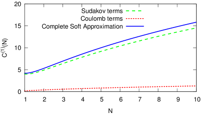
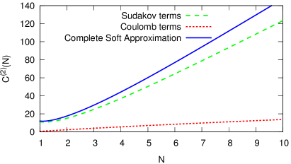
Figure 1: The contributions to $C(N)$ from soft gluon emission $\exp\left[G_{\mathbf{I}}(N,\alpha_{s})\right]$ (Sudakov terms) and Coulomb terms $J_{\mathbf{I}}(N,\alpha_{s})$ (Coulomb terms), at NLO (left) and NNLO (right). The combined effect Eq. (3.9) is also shown (Complete soft approximation).

A complete resummed expression of Coulomb contributions has been obtained in the context of potential non-relativistic QCD (pNRQCD) Brambilla:1999xf ; Beneke:2011mq ; Pineda:2006ri . This calculation can be used to test whether the pattern observed at NLO and NNLO continues at higher orders. In Fig. 2 we present the same comparison as in Fig. 1 at N³LO, with $J_{\mathbf{I}}^{(3)}(N)$ extracted from pNRQCD calculations Brambilla:1999xf ; Beneke:2011mq ; Pineda:2006ri . The effect of the inclusion of the $\mathcal{O}(\alpha_{s}^{3})$ term in $J_{\mathbf{I}}(N,\alpha_{s})$ as predicted by pNRQCD computations is indeed very small. We will include $J_{\mathbf{I}}^{(3)}(N)$ as computed by pNRQCD methods in our results, but these observations show that our final results are not significantly affected by it. An explicit form for all the Coulomb corrections is given in Appendix A, Eq. (A.12) (see also Ref. Muselli:tesi ).

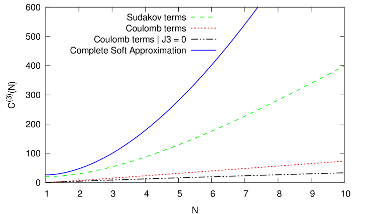
Figure 2: Same as Fig. 1 but at N³LO. The two different Coulomb curves differ by the inclusion of the pNRQCD estimate of $J_{\mathbf{I}}^{\left(3\right)}$ (see text).

3.3 Final prescription for the soft contribution

We conclude this section by giving our final prediction for the soft-emission contribution to the total cross section to N³LO. We define

$$C_{\text{A-soft}_{0}}(N) =\sum_{\mathbf{I=1,8}}\bar{g}_{\mathbf{I}}(\alpha_{s})J_{\mathbf{I}}(N,\alpha_{s})$$

$$\exp\left\{\sum_{n=1}^{\infty}\alpha_{s}^{n}\left[\sum_{k=0}^{n}b^{(A)}_{n,k}\hat{\mathcal{D}}_{k}\left(N\right)+\sum_{k=0}^{n-1}b^{(D)}_{n,k,\mathbf{I}}\hat{\mathcal{D}}_{k}(N)\right]\right\};$$ (3.11)

$$C_{\text{A-soft}_{1}}(N) =\sum_{\mathbf{I=1,8}}\bar{g}_{\mathbf{I}}(\alpha_{s})J_{\mathbf{I}}(N,\alpha_{s})$$

$$\exp\left\{\sum_{n=1}^{\infty}\alpha_{s}^{n}\left[\sum_{k=0}^{n}b^{(A)}_{n,k}\hat{\mathcal{D}}_{k}(N+1)+\sum_{k=0}^{n-1}b^{(D)}_{n,k,\mathbf{I}}\hat{\mathcal{D}}_{k}(N)\right]\right\}$$ (3.12)

where we have made explicit the dependence on $\alpha_{s}=\alpha_{s}(m^{2})$ and it is understood that the exponentials should be expanded in powers of $\alpha_{s}$ up to order $\alpha_{s}^{3}$. We will take the average between the two approximations,

$$C_{\text{A-soft}}(N)=\frac{1}{2}\left[C_{\text{A-soft}_{1}}(N)+C_{\text{A-soft}_{0}}(N)\right]$$ (3.13)

as the central value of our prediction, and the difference

$$\Delta^{\mathrm{soft}}(N)=\left|C_{\text{A-soft}_{1}}(N)-C_{\text{A-soft}_{0}}(N)\right|$$ (3.14)

as an estimate of the uncertainty of our procedure. Hence, our soft approximation to the coefficient function will be finally given by

$$C(N)=C_{\text{A-soft}}\pm\frac{\Delta^{\rm soft}}{2}.$$ (3.15)

We also consider the result which corresponds to the standard resummation, as given to NLL in Ref. Bonciani:1998vc , and extended to NNLL in Ref. Czakon:2013goa (and in the associate public code top++), which is expressed as a function of positive powers of $\ln N$, which we will call $N$-soft, following Ref. Ball:2013bra . This is given by

$$C_{N\text{-soft}}(N) =\sum_{\mathbf{I=1,8}}g_{\mathbf{I}}(\alpha_{s})J_{\mathbf{I}}(N,\alpha_{s})$$

$$\exp\left\{\sum_{n=1}^{\infty}\alpha_{s}^{n}\left[\sum_{k=0}^{n}b^{(A)}_{n,k}\mathcal{D}^{\text{log}}_{k}\left(N\right)+\sum_{k=0}^{n-1}b^{(D)}_{n,k,\mathbf{I}}\mathcal{D}^{\text{log}}_{k}(N)\right]\right\},$$ (3.16)

where the functions $\mathcal{D}^{\text{log}}_{k}(N)$ are the large $N$ limit of $\mathcal{D}_{k}(N)$ written in terms of positive powers of $\ln N$, excluding constants (for an explicit definition, see Ref. Ball:2013bra ), i.e. such that

$$\mathcal{D}_{k}(N)=\mathcal{D}^{\text{log}}_{k}(N)+d_{k}+\mathcal{O}\left(\frac{1}{N}\right),$$ (3.17)

thereby leading to

$$g_{\mathbf{I}}(\alpha_{s})=\bar{g}_{\mathbf{I}}(\alpha_{s})\exp\left[\sum_{n=1}^{3}\alpha_{s}^{n}\left(\sum_{k=0}^{n}b^{(A)}_{n,k}d_{k}+\sum_{k=0}^{n-1}b^{(D)}_{n,k,\mathbf{I}}d_{k}\right)\right].$$ (3.18)

4 Small-$N$ contributions

In order to extract the leading small-$N$ singularity of the partonic cross section, we will use the so-called high-energy or $k_{\rm\scriptscriptstyle\rm T}$ factorization technique, first described in Ref. Catani:1990eg for the total cross section, and more recently extended to rapidity distributions Ball:1999sh . We follow the resummation procedure developed by Altarelli, Ball and Forte (ABF) Altarelli:2008aj . For a detailed derivation of resummation, which affects both coefficient functions and evolution of the parton densities, we refer the reader to the original literature (e.g. Catani:1990eg ; Catani:1993ww ; Altarelli:2008aj ; Altarelli:2005ni ); here we only summarize the main results which are relevant for our discussion.

In the $k_{\rm\scriptscriptstyle\rm T}$ factorization formalism, small-$N$ singularities are obtained by computing the leading-order partonic cross section for the relevant process, with off-shell incoming gluons. We therefore define an off-shell partonic cross section $\frac{\alpha_{s}^{2}}{m^{2}}\hat{\sigma}_{\text{off-shell}}(\rho,\xi_{1},\xi_{2})$, which is a function of the scaling variable of the process $\rho$, and of the transverse momenta of the two off-shell gluons: $\xi_{i}={k^{2}_{\scriptscriptstyle\rm T}}_{i}/m^{2}$. Resummed results can be obtained through the determination of the so-called impact factor

$$h(N,M_{1},M_{2},m^{2},\alpha_{s}) =M_{1}M_{2}R(M_{1})R(M_{2})\left(\frac{m^{2}}{\mu_{\rm\scriptscriptstyle\rm F}^{2}}\right)^{M_{1}+M_{2}}$$

$$\times\int_{0}^{1}d\rho\,\rho^{N-2}\int_{0}^{\infty}d\xi_{1}\,\xi_{1}^{M_{1}-1}\int_{0}^{\infty}d\xi_{1}\,\xi_{1}^{M_{2}-1}\frac{\alpha_{s}^{2}}{m^{2}}\hat{\sigma}_{\text{off-shell}}(\rho,\xi_{1},\xi_{2}).$$ (4.1)

The prefactor $R(M_{1})R(M_{2})$ accounts for factorization scheme dependence Catani:1993ww ; in the $\overline{\rm MS}$ scheme

$$R(M)=1+\frac{8}{3}\zeta_{3}M^{3}+\mathcal{O}(M^{4}).$$ (4.2)

The impact factor Eq. (4.1) for the production of a heavy quark pair was computed in Ref. Ball:2001pq . Here, we are interested in its expansions in powers of $M_{1},M_{2}$, in the vicinity of $N=1$:

$$h(N,M_{1},M_{2},m^{2},\alpha_{s})=\frac{\alpha_{s}^{2}}{m^{2}}\sum_{i_{1},i_{2}}^{\infty}h_{i_{1},i_{2}}(\mu_{\rm\scriptscriptstyle\rm F}^{2})M_{1}^{i_{1}}M_{2}^{i_{2}}+\mathcal{O}(N-1).$$ (4.3)

The coefficients $h_{i_{1},i_{2}}$ relevant at N³LO can be easily obtained by performing the expansions of the previous formula and they are given in the Appendix B, Eq. (B.1). Following Refs. Ball:2007ra ; Altarelli:2008aj , the resummation is performed by identifying the Mellin variable $M_{i}$ with the resummed DGLAP anomalous dimension (together with sub-leading running-coupling effects):

$$M_{i}^{k}=\left[{\gamma_{\rm res}^{+}}^{k}\right],$$ (4.4)

where the right hand side is recursively defined by

$$\left[{\gamma_{\rm res}^{+}}^{k+1}\right]=\gamma_{\rm res}^{+}\left(1+k\frac{\dot{\gamma}_{\rm res}^{+}}{{\gamma_{\rm res}^{+}}^{2}}\right)\left[{\gamma_{\rm res}^{+}}^{k}\right],\quad\left[\gamma_{\rm res}^{+}\right]=\gamma_{\rm res}^{+}$$ (4.5)

with

$$\dot{\gamma}_{\rm res}^{+}=-\beta_{0}\alpha_{s}^{2}\frac{\partial}{\partial\alpha_{s}}\gamma_{\rm res}^{+}.$$ (4.6)

By expanding the anomalous dimension to fixed perturbative order

$$\gamma^{\rm\scriptscriptstyle\rm+}=\alpha_{s}\gamma^{(0)}+\alpha_{s}^{2}\gamma^{(1)}+\alpha_{s}^{3}\gamma^{(2)}+\mathcal{O}(\alpha_{s}^{4}),$$ (4.7)

we have all the ingredients to construct our $N\to 1$ approximation, which is simply found by substituting the expansion (4.7) in Eq. (4.5), and then in Eq. (4.3). The explicit form of the anomalous dimensions in the small-$N$ limit to the order relevant in our discussion is given in Appendix B, Eq. (B.2), (B.3) and (B.4). Now we define a resummed coefficient function by factoring out the leading order contribution, evaluated in the high-energy limit, i.e. $N=1$

$$C_{\scriptscriptstyle\rm ABF}(N) =\frac{\alpha_{s}^{2}}{m^{2}}\frac{1}{\hat{\sigma}^{\scriptscriptstyle\rm LO}(m^{2},1)}\left(\sum_{i_{1},i_{2}=0}^{\infty}h_{i_{1},i_{2}}\left[\gamma_{\rm res}^{+}\raisebox{6.88889pt}{$\scriptstyle i_{1}$}\right]\left[\gamma_{\rm res}^{+}\raisebox{6.88889pt}{$\scriptstyle i_{2}$}\right]\right)-1$$

$$=2\bar{h}_{1,0}\gamma^{\left(0\right)}+\alpha_{s}^{2}\left[\left(2\bar{h}_{2,0}+\bar{h}_{1,1}\right)\gamma^{(0)}\raisebox{6.88889pt}{$\scriptstyle 2$}-2\bar{h}_{2,0}\beta_{0}\gamma^{\left(0\right)}+2\bar{h}_{1,0}\gamma^{(1)}\right]$$

$$+\alpha_{s}^{3}\Big{[}\left(\bar{h}_{3,0}+\bar{h}_{2,1}\right)2\gamma^{(0)}\raisebox{6.88889pt}{$\scriptstyle 3$}-(3\bar{h}_{3,0}+\bar{h}_{2,1})2\beta_{0}\gamma^{(0)}\raisebox{6.88889pt}{$\scriptstyle 2$}+4\bar{h}_{3,0}\beta_{0}^{2}\gamma^{(0)}$$

$$\qquad+(2\bar{h}_{2,0}+\bar{h}_{1,1})2\gamma^{(0)}\gamma^{(1)}-4\bar{h}_{2,0}\beta_{0}\gamma^{(1)}+2\bar{h}_{1,0}\gamma^{(2)}\Big{]}+\mathcal{O}(\alpha_{s}^{4}),$$ (4.8)

where, in the second equality, we use the fact that

$$\hat{\sigma}^{\scriptscriptstyle\rm LO}(m^{2},1)=\frac{\alpha_{s}^{2}}{m^{2}}\,h_{0,0},$$ (4.9)

and we define

$$\bar{h}_{i_{1},i_{2}}=\frac{h_{i_{1},i_{2}}}{h_{0,0}}.$$ (4.10)

We have omitted the dependence of the coefficients on $\mu_{\rm\scriptscriptstyle\rm F}^{2}$ for simplicity.

Since we are going to combine the small-$N$ approximation with the large-$N$ approximation to obtain an estimate of the full coefficient function, we require that the two limiting behaviors do not interfere with each other. In particular, we require that the high-energy contribution vanishes when $N\to\infty$. Manifestly, Eq. (4.8) does not fulfil this requirement, because of the presence of a constant contribution in $\gamma^{(0)}$ (see Eq. (B.2) in Appendix B), which propagates in $C_{\scriptscriptstyle\rm ABF}(N)$ to all orders in $\alpha_{s}$. Therefore, following Ref. Ball:2013bra , we replace Eq. (4.8) with a modified version of the small-$N$ approximation to the partonic cross section, which has the same leading singularity in $N=1$ but vanishes as $N\to\infty$. The modified version is given by

$$C_{\scriptscriptstyle\rm\text{ABF-sub}}(N)=C_{\scriptscriptstyle\rm ABF}(N)-2C_{\scriptscriptstyle\rm ABF}(N+1)+C_{\scriptscriptstyle\rm ABF}(N+2).$$ (4.11)

The subtraction simply introduces subleading singularities in $N=0$ and $N=-1$, but now

$$\lim_{N\to\infty}C_{\scriptscriptstyle\rm\text{ABF-sub}}(N)=0$$ (4.12)

to all orders in $\alpha_{s}$. As pointed in Ref. Ball:2013bra , this choice for the subtraction is a compromise between the contrasting goals of not changing the small-$N$ singularities structure and of damping strongly enough as $N$ increases. In momentum space the subtraction of Eq. (4.11) corresponds to damping the $\rho\to 1$ behaviour of the partonic cross section through a multiplicative factor $(1-\rho)^{2}$.

One additional modification is needed to define our prediction for the cross section in the high-energy regime. We note that the anomalous dimensions vanishes at $N=2$ due to momentum conservation. This implies that the small-$N$ approximation Eq. (4.8) vanishes in $N=2$. This value of $N$ marks the transition between the small-$N$ approximation (not accurate if $N\gtrsim 2$) and the large-$N$ approximation (not accurate when $N\lesssim 2$).

However, Eq. (4.8), differs from $0$ in $N=2$ because the small-$N$ limit of the anomalous dimension $\gamma^{+}$, Eq. (4.7), contains only the leading and the next-to-leading singularities in $N=1$, and not a full fixed order expression. Momentum conservation can be enforced Altarelli:2008aj directly in Eq. (4.8), by adding to $C_{\scriptscriptstyle\rm ABF}(N)$ a function $f_{\rm mom}\propto 1/N$. Following Ref. Ball:2013bra , we construct our small-$N$ momentum-conserving approximation as

$$C_{\rm h.e}(N)=C_{\scriptscriptstyle\rm\text{ABF-sub}}(N)-\frac{4!k_{\rm mom}(\alpha_{s})}{N(N+1)(N+2)},$$ (4.13)

where the constant $k_{\rm mom}(\alpha_{s})$ is fixed by requiring that $C_{\rm h.e}(2)=0$ to all orders in the perturbative expansion. The enforcement of momentum conservation in our small-$N$ approximation allows us to estimate the contribution of subleading poles in $N=0,-1,-2,\dots$, which are not controlled by the high-energy approximation. Indeed, the full partonic cross section does not vanish at $N=2$: only the contribution to it driven by hard radiation from external legs does. Hence we can estimate subleading small-$N$ effects by allowing the partonic cross section to deviate slightly from zero at $N=2$ due to contributions from subleading poles. We thus fix $k_{\rm mom}$ to be

$$k_{\rm mom}(\alpha_{s})=C_{\scriptscriptstyle\rm\text{ABF-sub}}(2)\pm\Delta k_{\rm mom}(\alpha_{s}),$$ (4.14)

and we take the variation $\Delta k_{\rm mom}(\alpha_{s})$ to reach as its maximum value $15\%$ of the size of soft contribution $C_{\text{A-soft}}(N)$, Eq. (3.13) at $N=2$. This is a somewhat more conservative estimate of the uncertainty in comparison to the corresponding one adopted in Ref. Ball:2013bra , due to the fact that we expect the contribution from subleading poles to be potentially somewhat larger in this case, based on the behaviour of known orders, and possibly also due to the issues discussed in Sect. 2.2. Namely, we choose in Eq. (4.14),

$$\Delta k_{\rm mom}(\alpha_{s})=0.15\times C_{\text{A-soft}}(2).$$ (4.15)

In conclusion, this means that the small $N$ contribution, rather than being completely switched off at $N=2$, is small at this point, and gets switched off somewhere in its vicinity.

5 Approximate cross section up to N³LO

We are now ready to present our results for top pair production cross section at N³LO, by using Eq. (2.45) to combine the large-$N$ terms Eq. (3.15) and the small-$N$ terms Eq. (4.13). We first recall how $N$-space parton-level results can be related to physical hadron-level results using the saddle point methods, and then we present the parton and hadron level results in turn.

5.1 Saddle point approximation of Mellin inversion integrals

The physical hadronic cross section can be related to the underlying partonic cross section by viewing the former as the inverse Mellin transform of its factorized expression Eq. (2.6)

$$\sigma(m^{2},\rho_{h})=\frac{1}{2\pi i}\int_{c-i\infty}^{c+i\infty}dN\,\rho_{h}^{-N+1}\mathscr{L}(N)\hat{\sigma}(m^{2},N)=\frac{1}{2\pi i}\int_{c-i\infty}^{c+i\infty}dN\,\exp[f(N)],$$ (5.1)

where $c$ is to the right of all singularities of the integrand. It can be shown on general grounds that $f(N)$ has a unique minimum at $N=N_{0}$ on the real $N$ axis, which allows us to estimate the integral by the saddle-point technique.

The position $N_{0}$ of the saddle typically depends very weakly on the partonic cross section, and is mainly determined by the parton luminosity; the saddle-point approximation, with the inclusion of quadratic fluctuations around the saddle, turns out to be generally quite accurate Bonvini:2014qga . It is then possible to infer properties of the hadronic cross section from the behaviour of the partonic cross section at the value of $N$ which corresponds to the saddle point for given hadronic kinematics.

The position of the saddle point $N_{0}$ as a function of the collider energy $\sqrt{s}$, for $m=m_{t}=173.37$ GeV, computed using NNPDF 3.0 Ball:2014uwa parton distributions, is shown in Fig. 3.

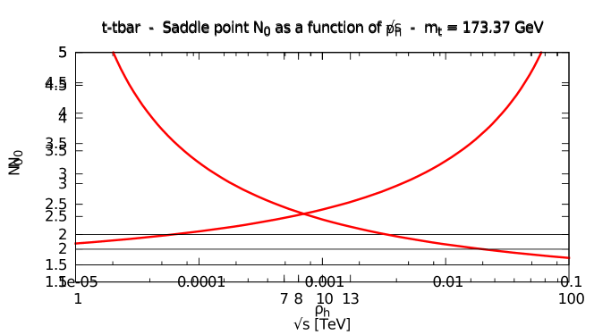
Figure 3: Position of the saddle point as a function of $\sqrt{s}$ for fixed top quark mass.

The value of the saddle turns out to be around $N=2.5$ at LHC energies. The value of $N_{0}$ is a very slowly decreasing function of the total energy.

5.2 Parton-level results

We can now combine the results of Sections 3 and 4 to obtain an estimate of the coefficients of the perturbative expansion for the total production cross section of heavy quark pairs. We first test our procedure against exact fixed-order calculations, which are available at NLO Nason:1987xz ; Czakon:2008ii and NNLO Czakon:2013goa . At NLO we specifically compare to the fit to the analytic result of Ref. Czakon:2008ii presented in Ref. Aliev:2010zk .

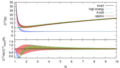
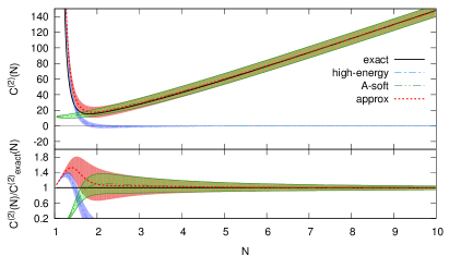
Figure 4: Comparison between exact results and our approximation at NLO (left) and NNLO (right) for the Mellin-space coefficient function $C(N)$; the large-$N$ contribution (A-soft) Eq.(3.15), the small-$N$ contribution (high-energy) Eq.(4.13), and the combined approximation of Eq. (2.45) (approx) are shown. The bottom plots show the ratio of the approximate to the exact result.

In Fig. 4 we show our approximation to the NLO and NNLO in Mellin space (labeled approx), compared to the exact results of Ref. Aliev:2010zk ; Czakon:2013goa . The large-$N$ contribution, $C_{\text{A-soft}}(N)$ Eq. (3.13) (labeled as soft), and the small-$N$ contribution, $C_{\rm h.e}(N)$ Eq. (4.13) (labeled as high-energy), are also shown. The renormalization and factorization scales are taken to be equal to the heavy quark mass $m$. The uncertainty on our prediction (red band) is obtained as the envelope of the uncertainty Eq. (3.15) on the soft terms (green band), and the uncertainty Eqs. (4.14), (4.15) on the high-energy terms (blue band).

The agreement is excellent at NLO in the whole range displayed in Fig. 4. At NNLO there is a slight discrepancy in the region between $1<N<1.6$. This is due to the fact we are only including the LL contribution in this region, while it was noted in Ref. Czakon:2013goa ; Czakon:2008ii that NLL contributions close to $N=1$ for top pair production are sizable. This region of $N$, however, would only be relevant for very high energy colliders ($\sqrt{s}\gtrsim 100$ TeV).

At the $N$ values which are relevant for LHC energies, the agreement between the approximate and exact results is excellent; for lower collider energy, as the saddle point moves towards larger values, the uncertainty on the approximate prediction is smaller.

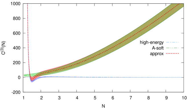
Figure 5: Same as Fig. 4, but at N³LO.

We now turn to the N³LO contribution. We recall that the constants $\bar{g}_{\mathbf{I}}^{(3)}$, together with the difference between coefficients $D_{\mathbf{8}}^{(3)}$ and $D_{\mathbf{1}}^{(3)}$, are not known. They will be set to zero for the time being; the impact of this missing information on our prediction for the physical cross section will be discussed in Section. 5.4 below. The function $C_{\rm approx}^{(3)}(N)$ is plotted in Fig. 5, together with the soft and the high-energy contributions that go into it according to Eq. (2.45).

5.3 Hadron-level results

We come now to the hadronic cross sections. It is convenient to define the gluon-channel $K$-factors

$$K_{gg}(m^{2},\rho_{h})=\frac{\sigma_{gg}(m^{2},\rho_{h})}{\sigma_{gg}^{\scriptscriptstyle\rm LO}(m^{2},\rho_{h})}=1+\alpha_{s}K_{gg}^{(1)}+\alpha_{s}^{2}K_{gg}^{(2)}+\alpha_{s}^{3}K_{gg}^{(3)}+\mathcal{O}(\alpha_{s}^{4}),$$ (5.2)

where $\alpha_{s}=\alpha_{s}(m^{2})$, $\sigma_{gg}(m^{2},\rho_{h})$ is the contribution to the hadron-level cross section Eq. (2.1) from the gluon-gluon subprocess, and $\sigma_{gg}^{\mathrm{LO}}(m^{2},\rho_{h})$ the corresponding leading-order approximation. All results will be obtained using the partonic cross sections of Sect. 5.2, with factorization and renormalization scale $\mu_{\rm\scriptscriptstyle\rm R}=\mu_{\rm\scriptscriptstyle\rm F}=m$, and NNPDF $3.0$ NNLO parton distribution functions Ball:2014uwa , with $\alpha_{s}(M^{2}_{Z})=0.118$ and $n_{f}=5$. Scale uncertainties on our final results will be discussed in Sect. 5.4 below.

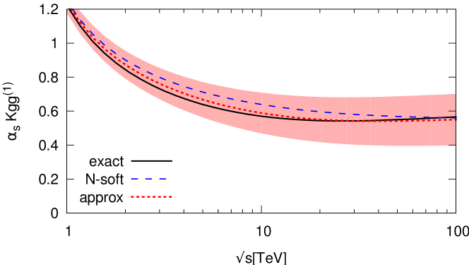
Figure 6: Comparison between the exact result and our approximation for the NLO contribution to the $K$-factor Eq. (5.2) from the gluon channel, plotted as a function of the collider energy $\sqrt{s}$. The result obtained expanding the standard NNLL resummation ($N$-soft) is also shown.

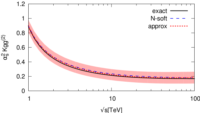
Figure 7: Same as Fig. 6 at NNLO.

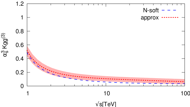
Figure 8: Same as Fig. 6 at N³LO, where the exact result is not known.

The NLO and NNLO $K$-factors at a $pp$ collider are shown in Figs. 6 and 7, respectively, as functions of the center-of-mass energy $\sqrt{s}$, and compared to the exact results of Ref. Aliev:2010zk ; Czakon:2013goa . We also show the values obtained by expanding out to the given order the standard resummed result of Refs. Bonciani:1998vc ; Czakon:2013goa , i.e. using the $N$-soft approximation Eq. (3.16). The main result of this work, namely the N³LO contribution to the $K$-factor in the gluon-gluon channel as a function of the collider energy is shown in Fig. 8. Numerical results for the $K$-factors at LHC energies are collected in Tab. 1.

		$\alpha_{s}(m^{2})K_{gg}^{(1)}$	$\alpha_{s}^{2}(m^{2})K_{gg}^{(2)}$	$\alpha_{s}^{3}(m^{2})K_{gg}^{(3)}$
$7$ TeV	exact	0.599	0.237
	approx	$0.623\pm 0.112$	$0.250\pm 0.076$	$0.098\pm 0.038$
	$N$-soft	0.672	0.260	0.056
$8$ TeV	exact	0.587	0.227
	approx	$0.609\pm 0.115$	$0.239\pm 0.076$	$0.094\pm 0.037$
	$N$-soft	0.658	0.250	0.052
$13$ TeV	exact	0.555	0.199
	approx	$0.569\pm 0.125$	$0.209\pm 0.077$	$0.083\pm 0.036$
	$N$-soft	0.619	0.221	0.040
$14$ TeV	exact	0.552	0.196
	approx	$0.565\pm 0.126$	$0.205\pm 0.077$	$0.082\pm 0.036$
	$N$-soft	0.614	0.217	0.038

Table 1: The NLO, NNLO, N³LO contributions the gluon channel $K$-factor at the LHC ($7$ TeV, $8$ TeV, $13$ TeV, $14$ TeV).

We note that our approximation reproduces the exact result within the estimated uncertainty both at NLO and at NNLO, in the whole energy range displayed in the plots. In comparison to the case of Higgs production, the uncertainty is larger, both because threshold resummation is known to a lower accuracy, and also because, as already mentioned, we have less control over $\frac{\ln^{k}N}{N}$ terms. Our result is seen to differ by varying amounts at each order from the $N$-soft one, simply obtained by expanding out the resummed result. At NLO and NNLO the origin of this difference is twofold: first, our approximation also includes the high-energy contribution and second, the functional form of the contribution obtained by expanding out the $N$-soft result differs from that adopted in our approximation, as explained in Sect. 3.3. At N³LO two further differences are, first, that our result includes the single logarithmic term, even if its coefficient is only partially known, which is absent in a NNLL resummation. However, the numerical impact of this contribution is small. Second, that the function of $\alpha_{s}$ which multiplies the resummed exponent is given by $g_{\mathbf{I}}(\alpha_{s})$ in the $N$-soft resummed result, and by $\bar{g}_{\mathbf{I}}(\alpha_{s})$ when constructing our approximation, the relation between the two being given by Eq. (3.18). We will specifically discuss the impact of this choice in the next Section (see in particular Tab. 2).

5.4 N³LO top pair production cross section at LHC

We collect now final results for top pair production at the LHC energies and its uncertainty. Our prediction for the total cross section with $\mu_{\rm\scriptscriptstyle\rm F}=\mu_{\rm\scriptscriptstyle\rm R}=m$ is

$$\textrm{LHC$7$:}\;\sigma^{\mathrm{N^{3}LO}}_{\mathrm{approx}}\left(\rho_{h},m^{2}\right) =\left(177.43\pm 2.99+0.10\,\bar{g}^{(3)}-0.10\,\left(D_{\mathbf{8}}^{(3)}-D_{\mathbf{1}}^{(3)}\right)\right)\,\textrm{pb},$$ (5.3a)

$$\textrm{LHC$8$:}\;\sigma^{\mathrm{N^{3}LO}}_{\mathrm{approx}}\left(\rho_{h},m^{2}\right) =\left(253.98\pm 4.35+0.14\,\bar{g}^{(3)}-0.14\,\left(D_{\mathbf{8}}^{(3)}-D_{\mathbf{1}}^{(3)}\right)\right)\,\textrm{pb},$$ (5.3b)

$$\textrm{LHC$13$:}\;\sigma^{\mathrm{N^{3}LO}}_{\mathrm{approx}}\left(\rho_{h},m^{2}\right) =\left(835.61\pm 14.78+0.51\,\bar{g}^{(3)}-0.46\,\left(D_{\mathbf{8}}^{(3)}-D_{\mathbf{1}}^{(3)}\right)\right)\,\textrm{pb},$$ (5.3c)

$$\textrm{LHC$14$:}\;\sigma^{\mathrm{N^{3}LO}}_{\mathrm{approx}}\left(\rho_{h},m^{2}\right) =\left(988.57\pm 17.55+0.61\,\bar{g}^{(3)}-0.54\,\left(D_{\mathbf{8}}^{(3)}-D_{\mathbf{1}}^{(3)}\right)\right)\,\textrm{pb},$$ (5.3d)

where

$$\bar{g}^{(i)}=\bar{g}_{\mathbf{1}}^{(i)}+\bar{g}_{\mathbf{8}}^{(i)}.$$ (5.4)

The constant $\bar{g}^{(3)}$ is not known. The difference between the coefficients $D_{\mathbf{8}}^{(3)}$ and $D_{\mathbf{1}}^{(3)}$ parametrizes the missing information about the single log at N³LO, as discussed in Section 3.1. Eq. (5.3) is obtained using exact expressions for the NLO Czakon:2008ii and NNLO Czakon:2013goa ; Baernreuther:2012ny ; Czakon:2012pz ; Czakon:2012zr , combined with our approximation for the N³LO in the gluon channel.

	$D_{\mathbf{8}}^{(i)}-D_{\mathbf{1}}^{(i)}$	$\bar{g}^{(i)}$	$g^{(i)}$	$g^{(i)}-\bar{g}^{(i)}$
$\alpha_{s}$	$-0.955$	$1.188$	$3.832$	$2.644$
$\alpha_{s}^{2}$	$-1.782$	$0.535$	$8.512$	$7.977$
$\alpha_{s}^{3}$	?	?	?	$12.348$

Table 2: The coefficients $D_{\mathbf{8}}^{(i)}-D_{\mathbf{1}}^{(i)}$, $\bar{g}^{(i)}$, $g^{(i)}$ and the difference between the latter two at NLO and NNLO.

We now consider various sources of uncertainty. First, we consider the uncertainty related to missing coefficients. In Tab. 2, we list the values of the coefficients $\bar{g}^{(i)}$, and of $D_{\mathbf{8}}^{(i)}-D_{\mathbf{1}}^{(i)}$ for the two known orders, as well as the coefficients $g^{(i)}$ defined using the analogue of Eq. (5.4) but for the expansion coefficients of $g_{\mathbf{I}}(\alpha_{s})$ Eq. (3.18) which is used in the standard resummed results of Refs. Bonciani:1998vc ; Czakon:2013goa , and the difference between the two, which is known to a higher perturbative order. Based on these values, we note that the perturbative behaviour of the coefficients $\bar{g}^{(i)}$ appears to be rather more stable than that of the coefficients $g^{(i)}$, and we reasonably expect the unknown coefficients, $\bar{g}^{(3)}$ and $D_{\mathbf{8}}^{(3)}-D_{\mathbf{1}}^{(3)}$, to be both of $\mathcal{O}(1)$. We conservatively estimate the uncertainty related to these unknown coefficients as

$$\bar{g}^{(3)}=0\pm 5,\qquad D_{\mathbf{8}}^{(3)}-D_{\mathbf{1}}^{(3)}=0\pm 10,$$ (5.5)

which we add in quadrature to the approximation uncertainty of Eq. (5.3). We also note in passing that the $N$-soft approximation assumes $g^{(3)}=0$, while our estimate corresponds to a value of order ten for this constant, thereby partly explaining the difference observed in Fig. 8 between our result and the $N$-soft approximation, as discussed in the previous Section.

A second source of uncertainty is due to the fact that we only predict the contribution of the gluon channel.

LHC$8$	$\sigma_{q\bar{q}}(pb)$	$\sigma_{qg}(pb)$	$\sigma_{gg}(pb)$
LO	$29.94$	$0$	$116.33$
NLO	$4.17$	$-0.45$	$66.66$
NNLO	$2.17$	$-2.30$	$26.36$

Table 3: Comparison of contributions to top pair production cross section from different channel at LHC 8 TeV at LO, NLO, NNLO.

In Tab. 3, we show the contributions to the top-pair production cross section coming from different partonic channels at LO, NLO, NNLO, for the specific case of LHC at $8$ TeV. We note that gluon fusion contribution is always dominant, and largely dominant at high perturbative orders. This remains true for other LHC energies (while at the Tevatron the $q\bar{q}$ component becomes dominant). Therefore, we expect that our estimate for the N³LO contribution based on the $gg$ channel only is only mildly affected by the lack of knowledge of the other channels. However, in order to take into account the uncertainty due to the missing partonic channels, we consider the dependence of our result on the factorization scale. Indeed, all the scale dependent terms at N³LO are available (for all channels), but the inclusion of all of them would consistently make the residual scale dependence of relative order $\alpha_{s}^{4}$. On the other hand, if we include $\mu_{\rm\scriptscriptstyle\rm F}$ dependent terms only in the $gg$ channel, the residual scale dependence is of order $\alpha_{s}^{3}$, since it misses the compensation between channels. The difference between these two ways of varying the scale can be thus taken as an estimate of the size of the contribution from the missing quark channels.

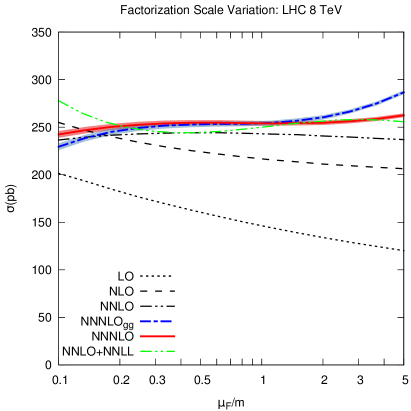
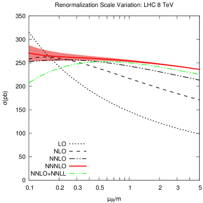
Figure 9: Factorization (left) and renormalization (right) scale dependence of the top production cross section at various perturbative orders. At N³LO the factorization scale dependence is shown both including the contribution from all channels (NNNLO) and from the gluon channel only (NNNLO_gg).

Finally, uncertainties related to missing higher-order terms can be estimated by varying the renormalization and factorization scales in the usual way. The dependence of the cross section at LO, NLO, NNLO and approximate N³LO on the factorization and renormalization scales, is shown in a wide range in Fig. 9; the NNLO+NNLL result of Refs Bonciani:1998vc ; Czakon:2013goa is also shown. The factorization scale variation at N³LO with $\mu_{\rm\scriptscriptstyle\rm F}$ is shown both retaining contributions from all channels, and from the $gg$ channel only. The factorization scale dependence is rather mild already at NNLO, and even milder at approximate N³LO when all channels are included. When only the $gg$ channel is included, a stronger scale dependence is observed, particularly at the extremes of the range, where sizable contributions from the missing channels are generated. The renormalization scale dependence is somewhat stronger than the factorization scale dependence, but at N³LO it has flattened out almost completely, thereby indicating a good perturbative convergence. It is interesting to observe that the NNLO+NNLL result has a milder scale dependence than the NNLO, but still a stronger scale dependence than the approximate N³LO. This is what one may expect based on the observation that effectively, because the process is far from threshold, the resummation is providing some approximation mostly to N³LO, which is however less complete than the approximation which is constructed here.

Our final results, with full uncertainty, are thus

$$\textrm{LHC$7$:}\;\sigma^{\mathrm{N^{3}LO}}_{\mathrm{approx}} =177.43\,\textrm{pb}\pm 1.79\%\text{(approx)}\pm 0.97\%\text{(channels)}{}^{+3.02\%}_{-2.87\%}\text{(scales)}$$ (5.6a)

$$\textrm{LHC$8$:}\;\sigma^{\mathrm{N^{3}LO}}_{\mathrm{approx}} =253.98\,\textrm{pb}\pm 1.82\%\text{(approx)}\pm 0.96\%\text{(channels)}{}^{+2.98\%}_{-2.83\%}\text{(scales)}$$ (5.6b)

$$\textrm{LHC$13$:}\;\sigma^{\mathrm{N^{3}LO}}_{\mathrm{approx}} =835.61\,\textrm{pb}\pm 1.88\%\text{(approx)}\pm 0.96\%\text{(channels)}{}^{+2.73\%}_{-2.65\%}\text{(scales)}$$ (5.6c)

$$\textrm{LHC$14$:}\;\sigma^{\mathrm{N^{3}LO}}_{\mathrm{approx}} =988.57\,\textrm{pb}\pm 1.88\%\text{(approx)}\pm 0.97\%\text{(channels)}{}^{+2.68\%}_{-2.62\%}\text{(scales)}$$ (5.6d)

where the “channels” uncertainty has been computed as ($\pm$ half) the difference between the $\mu_{\rm\scriptscriptstyle\rm F}$ scale variation evaluated with only the $gg$ channel or with all the channels (NNNLO_gg and NNNLO curves in Fig. 9), in the range $m/2\leq\mu_{\rm\scriptscriptstyle\rm F}\leq 2m$ with $\mu_{\rm\scriptscriptstyle\rm R}=m$. The “scales” uncertainty is instead obtained through a canonical seven-point variation, namely $m/2\leq\mu_{\rm\scriptscriptstyle\rm R},\mu_{\rm\scriptscriptstyle\rm F}\leq 2m$ with $1/2\leq\mu_{\rm\scriptscriptstyle\rm R}/\mu_{\rm\scriptscriptstyle\rm F}\leq 2$, computed with all channels. We observe that the approximation uncertainties, though conservatively estimated, are rather smaller than the scale uncertainty, and in fact adding in quadrature scale and approximation uncertainties we end up with an overall theoretical uncertainty on our N³LO result of $3.5\%$, not much larger than the scale uncertainty itself. This uncertainties can be compared to the PDF uncertainty, which at the LHC $\sqrt{s}=13$ TeV (with NNPDF 3.0 PDFs) is of order $2\%$. Additional uncertainties come from the values of $\alpha_{s}$ and $m_{t}$: see Ref. Czakon:2013tha for a more detailed discussion.

We observe that the uncertainty due to scale variations at NNLO is about 5% at the collider energies we are considering, which is larger than the overall uncertainty on our N³LO estimate even accounting for approximation uncertainties. The inclusion of our approximate N³LO contribution appears thus to be advantageous, and it leads to a decrease in theoretical uncertainty which is of the size one would expect when going ftom NNLO to N³LO.

We may compare our approximate N³LO result to that which would be obtained using the $N$-soft result shown in Fig. 8. The latter leads to a N³LO contribution which corresponds to an increase of $3\%,2.8\%,2.3\%,2.4\%$ in comparison to the NNLO at LHC $\sqrt{s}=7,8,13,14$ TeV, respectively. This is rather lower than our approximate result, which corresponds to an increase of $4.3\%,4.5\%,4.2\%,4.3\%$ respectively. The reasons for this have been discussed in the previous section. As discussed above, and as it is apparent from Fig. 9, the scale uncertainty on this result is somewhat smaller than that on the NNLO result, but larger than that on our result.

Finally, we note that an approximate N³LO result is also presentes in Ref. Kidonakis:2014isa . This result is obtained by considering logarithmic terms enhanced at partonic threshold in the differential cross section, inclusive in one of the two heavy quarks produced. The result is then integrated to obtain the inclusive cross section. The enhancements over the NNLO results were found to be $4\%,3.6\%,2.7\%,2.6\%$ at $\sqrt{s}=7,8,13,14$ TeV respectively. We leave a more detailed comparison to the results of Ref. Kidonakis:2014isa , as well as to the resummed result obtained in SCET (e.g. Refs. Beneke:2009ye ; Beneke:2010da and Refs. Ahrens:2010zv ; Ahrens:2011px ; Yang:2014hya ), for future work.

6 Conclusions

We have constructed an approximate expression for the N³LO contribution to the production cross section of a heavy-quark pair at hadron-hadron colliders. We have focused on the gluon-gluon initiated subprocess, which gives the largest contribution at the LHC.

We have obtained our result by extending the method developed by some of us for the case of Higgs production in gluon-gluon fusion Ball:2013bra , and based on reconstructing the Mellin-space partonic cross section from its known singularities. Heavy-quark production is a process with a rather more complicated kinematic and color structure compared to inclusive Higgs production. Furthermore, fixed-order coefficient function for this process are known to have a rather non-trivial singularity structure in physical space, at first sight unrelated to the threshold or high-energy limits. Therefore, application to this case of the the technique suggested in Ref. Ball:2013bra and applied there to Higgs production in gluon fusion provides a rather stringent test of this methodology. In this study we have shown that the method of Ref. Ball:2013bra provides excellent approximations to known results up to NNLO, thereby validating he methodology.

Having established the reliability of the methodology even in this more subtle case, we have used it to produce a N³LO approximate partonic cross section for heavy quark production. We have then focused on the $t\bar{t}$ cross section, which is of great interest at the LHC. We have found that the approximate N³LO correction amounts to an increase in comparison to the NNLO prediction of $4.3\%,4.5\%,4.2\%,4.3\%$, for $pp$ collisions at $\sqrt{s}=7,8,13,14$ TeV, respectively. Inclusion of this correction reduces the scale uncertainty to 3%, with a combined uncertainty on the approximation itself of comparable size or smaller. Our final overall conservatively estimated uncertainty is thus somewhat smaller than the uncertainty on the exactly known NNLO result, and inclusion of our approximate result appears to be advantageous.

Appendix A Coefficients in the large-$N$ contribution

The coefficients $b^{(A)}_{n,k}(\mu_{\rm\scriptscriptstyle\rm F}^{2})$ and $b^{(D)}_{n,k,\mathbf{I}}(\mu_{\rm\scriptscriptstyle\rm F}^{2})$ defined in Eq. (3.1) for $n\leq 3$ are given by

$$b^{(A)}_{1,0} =4A^{(1)}\ln 2+2A^{(1)}\ln\frac{m^{2}}{\mu_{\rm\scriptscriptstyle\rm F}^{2}}$$ (A.1a)

$$b^{(A)}_{1,1} =4A^{(1)}$$ (A.1b)

$$b^{(A)}_{2,0} =4A^{(2)}\ln 2-4A^{(1)}\beta_{0}\ln^{2}2+2A^{(2)}\ln\frac{m^{2}}{\mu_{\rm\scriptscriptstyle\rm F}^{2}}+A^{(1)}\beta_{0}\ln^{2}\frac{m^{2}}{\mu_{\rm\scriptscriptstyle\rm F}^{2}}$$ (A.1c)

$$b^{(A)}_{2,1} =4A^{(2)}-8A^{(1)}\beta_{0}\ln 2$$ (A.1d)

$$b^{(A)}_{2,2} =-4A^{(1)}\beta_{0}$$ (A.1e)

$$b^{(A)}_{3,0} =4A^{(3)}\ln 2-8A^{(2)}\beta_{0}\ln^{2}2-4A^{(1)}\beta_{1}\ln^{2}2+\frac{16}{3}A^{(1)}\beta^{2}_{0}\ln^{3}2$$

$$+2A^{(3)}\ln\frac{m^{2}}{\mu_{\rm\scriptscriptstyle\rm F}^{2}}+\left(2A^{(2)}\beta_{0}+A^{(1)}\beta_{1}\right)\ln^{2}\frac{m^{2}}{\mu_{\rm\scriptscriptstyle\rm F}^{2}}+\frac{2}{3}A^{(1)}\beta_{0}^{2}\ln^{3}\frac{m^{2}}{\mu_{\rm\scriptscriptstyle\rm F}^{2}}$$ (A.1f)

$$b^{(A)}_{3,1} =4A^{(3)}-16A^{(2)}\beta_{0}\ln 2-8A^{(1)}\beta_{1}\ln 2+16A^{(1)}\beta_{0}^{2}\ln^{2}2$$ (A.1g)

$$b^{(A)}_{3,2} =-8A^{(2)}\beta_{0}-4A^{(1)}\beta_{1}+16A^{(1)}\beta_{0}^{2}\ln 2$$ (A.1h)

$$b^{(A)}_{3,3} =\frac{16}{3}A^{(1)}\beta_{0}^{2}$$ (A.1i)

and

$$b^{(D)}_{1,0,\mathbf{I}} =D_{\mathbf{I}}^{(1)}$$ (A.2a)

$$b^{(D)}_{2,0,\mathbf{I}} =D_{\mathbf{I}}^{(2)}-2\beta_{0}D_{\mathbf{I}}^{(1)}\ln 2$$ (A.2b)

$$b^{(D)}_{2,1,\mathbf{I}} =-2\beta_{0}D_{\mathbf{I}}^{(1)}$$ (A.2c)

$$b^{(D)}_{3,0,\mathbf{I}} =D_{\mathbf{I}}^{\left(3\right)}-2\beta_{1}D_{\mathbf{I}}^{(1)}\ln 2-4\beta_{0}D_{\mathbf{I}}^{\left(2\right)}\ln 2+4\beta_{0}^{2}D_{\mathbf{I}}^{(1)}\ln^{2}2$$ (A.2d)

$$b^{(D)}_{3,1,\mathbf{I}} =-2\beta_{1}D_{\mathbf{I}}^{(1)}-4\beta_{0}D_{\mathbf{I}}^{\left(2\right)}+8\beta_{0}^{2}D_{\mathbf{I}}^{(1)}\ln 2$$ (A.2e)

$$b^{(D)}_{3,2,\mathbf{I}} =4\beta_{0}^{2}D_{\mathbf{I}}^{(1)}$$ (A.2f)

where

$$A\left(\alpha_{s}\right) =A^{(1)}\alpha_{s}+A^{(2)}\alpha_{s}^{2}+A^{(3)}\alpha_{s}^{3}+\mathcal{O}\left(\alpha_{s}^{4}\right);$$ (A.3a)

$$A^{(1)} =\frac{C_{\rm\scriptscriptstyle\rm A}}{\pi}$$ (A.3b)

$$A^{(2)} =\frac{C_{\rm\scriptscriptstyle\rm A}}{2\pi^{2}}\left(\left(\frac{67}{18}-\zeta_{2}\right)C_{\rm\scriptscriptstyle\rm A}-\frac{5}{9}n_{f}\right)$$ (A.3c)

$$A^{(3)} =\frac{C_{\rm\scriptscriptstyle\rm A}}{4\pi^{3}}\Big{(}C_{\rm\scriptscriptstyle\rm A}^{2}\left(\frac{245}{24}-\frac{67}{9}\zeta_{2}+\frac{11}{6}\zeta_{3}+\frac{11}{5}\zeta_{2}^{2}\right)$$

$$+C_{\rm\scriptscriptstyle\rm F}n_{f}\left(-\frac{55}{24}+2\zeta_{3}\right)+C_{\rm\scriptscriptstyle\rm A}n_{f}\left(-\frac{209}{108}+\frac{10}{9}\zeta_{2}-\frac{7}{3}\zeta_{3}\right)-\frac{n_{f}^{2}}{27}\Big{)}$$ (A.3d)

and

$$D_{\mathbf{I}}\left(\alpha_{s}\right) =D_{\mathbf{I}}^{(1)}\alpha_{s}+D_{\mathbf{I}}^{(2)}\alpha_{s}^{2}+D_{\mathbf{I}}^{(3)}\alpha_{s}^{3}+\mathcal{O}\left(\alpha_{s}^{4}\right);$$ (A.4a)

$$D_{\mathbf{1}}^{(1)} =0$$ (A.4b)

$$D_{\mathbf{1}}^{(2)} =\frac{C_{\rm\scriptscriptstyle\rm A}}{\pi^{2}}\left(\left(-\frac{101}{27}+\frac{11}{18}\pi^{2}+\frac{7}{2}\zeta_{3}\right)C_{\rm\scriptscriptstyle\rm A}+\left(\frac{14}{27}-\frac{\pi^{2}}{9}\right)n_{f}\right)$$ (A.4c)

$$D_{\mathbf{1}}^{(3)} =\frac{1}{\left(4\pi\right)^{3}}\Big{(}C_{\rm\scriptscriptstyle\rm A}^{3}\left(-\frac{594058}{729}+\frac{98224}{81}\zeta_{2}+\frac{40144}{27}\zeta_{3}-\frac{2992}{15}\zeta_{2}^{2}-\frac{352}{3}\zeta_{2}\zeta_{3}-384\zeta_{5}\right)$$

$$+C_{\rm\scriptscriptstyle\rm A}^{2}n_{f}\left(\frac{125252}{729}-\frac{29392}{81}\zeta_{2}-\frac{2480}{9}\zeta_{3}+\frac{736}{15}\zeta_{2}^{2}\right)$$

$$+C_{\rm\scriptscriptstyle\rm A}C_{\rm\scriptscriptstyle\rm F}n_{f}\left(\frac{3422}{27}-32\zeta_{2}-\frac{608}{9}\zeta_{3}-\frac{64}{5}\zeta_{2}^{2}\right)$$

$$+C_{\rm\scriptscriptstyle\rm A}n_{f}^{2}\left(-\frac{3712}{729}+\frac{640}{27}\zeta_{2}+\frac{320}{27}\zeta_{3}\right)\Big{)}$$ (A.4d)

$$D_{\mathbf{8}}^{(1)} =D_{\mathbf{1}}^{(1)}-\frac{C_{\rm\scriptscriptstyle\rm A}}{\pi}$$ (A.4e)

$$D_{\mathbf{8}}^{(2)} =D_{\mathbf{1}}^{(2)}+\frac{C_{\rm\scriptscriptstyle\rm A}}{36\pi^{2}}\left(C_{\rm\scriptscriptstyle\rm A}\left(-115+3\pi^{2}-18\zeta_{3}\right)+22n_{f}\right),$$ (A.4f)

while $D_{\mathbf{8}}^{(3)}$ is unknown.

To complete our resummed formula for the soft emission, we need explicit expressions for the functions $\hat{\mathcal{D}}_{k}(N)$, Mellin transforms of the distributions

$$\hat{\mathcal{D}}_{k}\left(z\right)=\left[\frac{\ln^{k}\left(1-z\right)}{1-z}\right]_{+}+\left[\frac{\ln^{k}\frac{1-z}{\sqrt{z}}}{1-z}-\frac{\ln^{k}\left(1-z\right)}{1-z}\right],$$ (A.5)

where the plus distribution is defined by

$$\int_{0}^{1}dz\,\left[f\left(z\right)\right]_{+}g\left(z\right)=\int_{0}^{1}dz\,g\left(z\right)\left[f\left(z\right)-f\left(1\right)\right].$$ (A.6)

The full calculation is presented for example in Ref. Bonvini:2012sh ; Ball:2013bra . Here we give the final result:

$$\hat{\mathcal{D}}_{k}\left(N\right)=\frac{1}{k+1}\sum_{j=0}^{k}\binom{k+1}{j}\Gamma^{\left(j\right)}\left(1\right)\left[\Upsilon^{\left(k+1-j\right)}\left(N,0\right)-\Delta^{\left(k+1-j\right)}\left(1\right)\right],$$ (A.7)

where we have defined

$$\Delta\left(\xi\right) =\frac{1}{\Gamma\left(\xi\right)}$$ (A.8)

$$\Upsilon\left(N,\xi\right) =\Gamma\left(N-\frac{\xi}{2}\right)\Delta\left(N+\frac{\xi}{2}\right),$$ (A.9)

$\Gamma(N)$ is the usual Euler function, and the superscript in round brackets in $\Upsilon\left(N,\xi\right)$ denotes differentiation with respect to $\xi$. For the first three values of $k$, relevant for our N³LO approximation, we find

$$\hat{\mathcal{D}}_{0}\left(N\right) =-L,$$ (A.10a)

$$\hat{\mathcal{D}}_{1}\left(N\right) =+\frac{1}{2}\left[L^{2}+\zeta_{2}\right],$$ (A.10b)

$$\hat{\mathcal{D}}_{2}\left(N\right) =-\frac{1}{3}\left[L^{3}+3\zeta_{2}L+2\zeta_{3}+\frac{1}{4}\psi_{2}(N)\right],$$ (A.10c)

$$\hat{\mathcal{D}}_{3}\left(N\right) =+\frac{1}{4}\left[L^{4}+6\zeta_{2}L^{2}+8\zeta_{3}L+\frac{27}{5}\zeta_{2}^{2}+\psi_{2}(N)L\right],$$ (A.10d)

with

$$L=\psi_{0}(N)+\gamma_{\scriptscriptstyle E},$$ (A.11)

where $\psi_{k}(N)=\psi_{0}^{(k)}(N)$, $\psi_{0}(N)=\Gamma^{\prime}(N)/\Gamma(N)$ are the usual polygamma functions and $\gamma_{\scriptscriptstyle E}=-\psi_{0}(1)$ is the Euler-Mascheroni constant.

The Coulomb functions $J_{\mathbf{I}}(N,\alpha_{s})$ are computed by taking a Mellin transform of the resummed momentum-space results obtained in the context of pNRQCD Beneke:2010da ; Beneke:1999qg . For more details about the procedure of this Mellin transformation, see Ref. Muselli:tesi . The explicit expression for the Coulomb functions, up to N³LO, is the following:

$$J_{\mathbf{I}}(N,\alpha_{s}) =1+J^{(1)}_{\mathbf{I}}(N)\alpha_{s}+J^{(2)}_{\mathbf{I}}(N)\alpha_{s}^{2}+J^{(3)}_{\mathbf{I}}(N)\alpha_{s}^{3}+\mathcal{O}(\alpha_{s}^{4})$$ (A.12a)

$$J_{\mathbf{1}}^{(1)}(N) =\frac{\pi C_{\rm\scriptscriptstyle\rm F}2^{1-2N}}{B\left(N,N\right)}$$ (A.12b)

$$J_{\mathbf{1}}^{(2)}(N) =\frac{C_{\rm\scriptscriptstyle\rm F}^{2}\pi^{2}}{6}\left(N-\frac{1}{2}\right)$$

$$-C_{\rm\scriptscriptstyle\rm F}\left(C_{\rm\scriptscriptstyle\rm F}+\frac{C_{\rm\scriptscriptstyle\rm A}}{2}\right)\left(-\gamma_{\scriptscriptstyle E}+2-2\left(\psi_{0}\left(2N\right)-\psi_{0}\left(N\right)\right)\right)$$

$$+\Bigg{(}\left(-\frac{11}{24}C_{\rm\scriptscriptstyle\rm F}C_{\rm\scriptscriptstyle\rm A}+\frac{C_{\rm\scriptscriptstyle\rm F}n_{f}}{12}\right)\left(\ln 2+\frac{1}{2}\left(-\gamma_{\scriptscriptstyle E}-\psi_{0}(N)\right)\right)$$

$$+\left(\frac{31}{72}C_{\rm\scriptscriptstyle\rm F}C_{\rm\scriptscriptstyle\rm A}-\frac{5}{36}C_{\rm\scriptscriptstyle\rm F}n_{f}\right)\Bigg{)}\frac{2^{2-2N}}{B\left(N,N\right)}$$ (A.12c)

$$J_{\mathbf{1}}^{(3)}(N) =\frac{C_{\rm\scriptscriptstyle\rm F}^{2}\pi}{108}\left(N-\frac{1}{2}\right)$$

$$\left(93-10n_{f}-432\frac{\beta_{0}\zeta_{3}}{\pi}+36\pi\beta_{0}\left(\gamma_{\scriptscriptstyle E}-2\ln 2+2\left(\psi_{0}\left(2N\right)-\psi_{0}\left(N\right)\right)\right)\right)$$

$$-\frac{C_{\rm\scriptscriptstyle\rm F}^{2}\pi}{108}+C_{\rm\scriptscriptstyle\rm F}^{2}\left(C_{\rm\scriptscriptstyle\rm A}+2C_{\rm\scriptscriptstyle\rm F}\right)\frac{\pi}{2^{2N}B\left(N,N\right)}\left(\gamma_{\scriptscriptstyle E}+\psi_{0}(N)\right)$$ (A.12d)

$$J_{\mathbf{8}}^{(1)}(N) =\frac{\pi\left(C_{\rm\scriptscriptstyle\rm F}-\frac{C_{\rm\scriptscriptstyle\rm A}}{2}\right)2^{1-2N}}{B\left(N,N\right)}$$ (A.12e)

$$J_{\mathbf{8}}^{(2)}(N) =\frac{\left(C_{\rm\scriptscriptstyle\rm F}-\frac{C_{\rm\scriptscriptstyle\rm A}}{2}\right)^{2}\pi^{2}}{6}\left(N-\frac{1}{2}\right)$$

$$-C_{\rm\scriptscriptstyle\rm F}\left(C_{\rm\scriptscriptstyle\rm F}-\frac{C_{\rm\scriptscriptstyle\rm A}}{2}\right)\left(-\gamma_{\scriptscriptstyle E}+2-2\left(\psi_{0}\left(2N\right)-\psi_{0}\left(N\right)\right)\right)$$

$$+\Bigg{(}\left(-\frac{11}{24}C_{\rm\scriptscriptstyle\rm A}+\frac{n_{f}}{12}\right)\left(C_{\rm\scriptscriptstyle\rm F}-\frac{C_{\rm\scriptscriptstyle\rm A}}{2}\right)\left(\ln 2+\frac{1}{2}\left(-\gamma_{\scriptscriptstyle E}-\psi_{0}(N)\right)\right)$$

$$+\left(\frac{31}{72}C_{\rm\scriptscriptstyle\rm A}-\frac{5}{36}n_{f}\right)\left(C_{\rm\scriptscriptstyle\rm F}-\frac{C_{\rm\scriptscriptstyle\rm A}}{2}\right)\Bigg{)}\frac{2^{2-2N}}{B\left(N,N\right)}$$ (A.12f)

$$J_{\mathbf{8}}^{(3)}(N) =\frac{\left(C_{\rm\scriptscriptstyle\rm F}-\frac{C_{\rm\scriptscriptstyle\rm A}}{2}\right)^{2}\pi}{108}\left(N-\frac{1}{2}\right)$$

$$\left(93-10n_{f}-432\frac{\beta_{0}\zeta_{3}}{\pi}+36\pi\beta_{0}\left(\gamma_{\scriptscriptstyle E}-2\ln 2+2\left(\psi_{0}\left(2N\right)-\psi_{0}\left(N\right)\right)\right)\right)$$

$$-\frac{\left(C_{\rm\scriptscriptstyle\rm F}-\frac{C_{\rm\scriptscriptstyle\rm A}}{2}\right)^{2}\pi}{108}+\frac{\left(2C_{\rm\scriptscriptstyle\rm F}-C_{\rm\scriptscriptstyle\rm A}\right)^{2}C_{\rm\scriptscriptstyle\rm F}\pi}{2^{2N-1}B\left(N,N\right)}\left(\gamma_{\scriptscriptstyle E}+\psi_{0}(N)\right).$$ (A.12g)

with $B\left(a,b\right)=\frac{\Gamma(a)\Gamma(b)}{\Gamma(a+b)}$ the Beta function.

We now turn to the functions $\bar{g}_{\mathbf{I}}(\alpha_{s})$. They must be computed by matching with exact results, which are available up to NNLO. Moreover, as pointed out in Ref. Czakon:2013goa , at NNLO we can only infer from the exact result the sum $\bar{g}^{(2)}=\bar{g}_{\mathbf{1}}^{(2)}+\bar{g}_{\mathbf{8}}^{(2)}$, but not the individual contributions $\bar{g}^{(2)}_{\mathbf{I}}$. The latter have been estimated by the same procedure adopted in Ref. Czakon:2013goa , giving

$$\bar{g}_{\mathbf{I}}(\alpha_{s})=1+\bar{g}_{\mathbf{I}}^{(1)}\alpha_{s}+\bar{g}_{\mathbf{I}}^{(2)}\alpha_{s}^{2}+\mathcal{O}\left(\alpha_{s}^{3}\right)$$ (A.13a)

$$\bar{g}_{\mathbf{1}}^{(1)}=\frac{2}{7\pi}\left[C_{\rm\scriptscriptstyle\rm F}\left(-5+\frac{\pi^{2}}{4}\right)+C_{\rm\scriptscriptstyle\rm A}\left(1+\frac{\pi^{2}}{12}\right)\right]$$ (A.13b)

$$\bar{g}_{\mathbf{1}}^{(2)}=0.216$$ (A.13c)

$$\bar{g}_{\mathbf{8}}^{(1)}=\frac{5}{7\pi}\left[C_{\rm\scriptscriptstyle\rm F}\left(-5+\frac{\pi^{2}}{4}\right)+C_{\rm\scriptscriptstyle\rm A}\left(3-\frac{\pi^{2}}{24}\right)\right]$$ (A.13d)

$$\bar{g}_{\mathbf{8}}^{(2)}=0.319.$$ (A.13e)

It can be checked that the uncertainty due to this additional guess is completely negligible in comparison to our error bands. For simplicity we do not give the explicit factorization scale dependence of $\bar{g}(\alpha_{s})$.

Appendix B Coefficients in the small-$N$ contribution

The only ingredients which are needed for the high-energy contribution are the coefficients $h_{i_{1},i_{2}}$ of the expansion of the impact factor, up to N³LO:

$$h_{0,0} =\frac{181\pi}{2160}$$ (B.1a)

$$h_{1,0} =h_{0,1}=\frac{7291\pi}{32400}$$ (B.1b)

$$h_{1,1} =\frac{502417\pi}{486000}-\frac{251\pi^{3}}{12960}$$ (B.1c)

$$h_{2,0} =h_{0,2}=\frac{58849\pi}{121500}$$ (B.1d)

$$h_{2,1} =h_{1,2}=\frac{\pi\left(47041256-700575\pi^{2}+7526250\zeta_{3}\right)}{14580000}$$ (B.1e)

$$h_{3,0} =h_{0,3}=\frac{\pi\left(3608438+203625\zeta_{3}\right)}{3645000}.$$ (B.1f)

The coefficients $\bar{h}_{i_{1},i_{2}}$ are simply obtained dividing each $h_{i_{1},i_{2}}$ by $h_{0,0}$. The factorization scale dependence can be easily restored following the procedure explained for example in Ref. Ball:2013bra .

The leading and next-to-leading singular contributions to the anomalous dimension $\gamma^{\rm\scriptscriptstyle\rm+}$ are

$$\gamma^{(0)} =\frac{e_{0,-1}}{N-1}+e_{0,0}+\mathcal{O}(N-1)$$ (B.2)

$$\gamma^{(1)} =\frac{e_{1,-2}}{(N-1)^{2}}+\frac{e_{1,-1}}{N-1}+\mathcal{O}(1)$$ (B.3)

$$\gamma^{(2)} =\frac{3_{2,-3}}{(N-1)^{3}}+\frac{e_{2,-2}}{(N-1)^{2}}+\mathcal{O}\left((N-1)^{-1}\right),$$ (B.4)

with $e_{0,-1}=\frac{C_{\rm\scriptscriptstyle\rm A}}{\pi}$, $e_{1,-2}=e_{2,-3}=0$ and

$$e_{0,0} =\frac{-11C_{\rm\scriptscriptstyle\rm A}^{2}+2n_{f}(2C_{\rm\scriptscriptstyle\rm F}-C_{\rm\scriptscriptstyle\rm A})}{12\pi C_{\rm\scriptscriptstyle\rm A}}$$ (B.5)

$$e_{1,-1} =\left(\frac{13C_{\rm\scriptscriptstyle\rm F}}{18\pi^{2}}-\frac{23C_{\rm\scriptscriptstyle\rm A}}{36\pi^{2}}\right)n_{f}$$ (B.6)

$$e_{2,-2} =\frac{C_{\rm\scriptscriptstyle\rm A}^{3}\zeta_{3}}{2\pi^{3}}+\frac{11C_{\rm\scriptscriptstyle\rm A}^{3}\zeta_{2}}{12\pi^{3}}-\frac{395C_{\rm\scriptscriptstyle\rm A}^{3}}{108\pi^{3}}+\left(\frac{C_{\rm\scriptscriptstyle\rm A}^{2}\zeta_{2}}{6\pi^{3}}-\frac{71C_{\rm\scriptscriptstyle\rm A}^{2}}{108\pi^{3}}-\frac{C_{\rm\scriptscriptstyle\rm F}C_{\rm\scriptscriptstyle\rm A}\zeta_{2}}{3\pi^{3}}+\frac{71C_{\rm\scriptscriptstyle\rm F}C_{\rm\scriptscriptstyle\rm A}}{54\pi^{3}}\right)n_{f}.$$ (B.7)

References

• (1) C. Anastasiou, C. Duhr, F. Dulat, F. Herzog and B. Mistlberger, arXiv:1503.06056 [hep-ph].
• (2) R. D. Ball, M. Bonvini, S. Forte, S. Marzani and G. Ridolfi, Nucl. Phys. B 874 (2013) 746 [arXiv:1303.3590 [hep-ph]].
• (3) M. Bonvini, R. D. Ball, S. Forte, S. Marzani and G. Ridolfi, J. Phys. G 41 (2014) 095002 [arXiv:1404.3204 [hep-ph]].
• (4) M. Bonvini and S. Marzani, JHEP 1409 (2014) 007 [arXiv:1405.3654 [hep-ph]].
• (5) M. Kramer, E. Laenen and M. Spira, Nucl. Phys. B 511 (1998) 523 [hep-ph/9611272].
• (6) P. Nason, S. Dawson and R. K. Ellis, Nucl. Phys. B 303 (1988) 607.
• (7) M. L. Mangano, P. Nason and G. Ridolfi, Nucl. Phys. B 373 (1992) 295. Nuclear Physics B373(1992).
• (8) M. Czakon and A. Mitov, Nucl. Phys. B 824 (2010) 111 [arXiv:0811.4119 [hep-ph]].
• (9) P. Baernreuther, M. Czakon and A. Mitov, arXiv:1206.0621 [hep-ph].
• (10) M. Czakon and A. Mitov, JHEP 1212 (2012) 054 [arXiv:1207.0236 [hep-ph]].
• (11) M. Czakon and A. Mitov, JHEP 1301 (2013) 080 [arXiv:1210.6832 [hep-ph]].
• (12) M. Czakon, P. Fiedler and A. Mitov, Phys. Rev. Lett.  110 (2013) 252004 [arXiv:1303.6254 [hep-ph]].
• (13) S. Moch, P. Uwer and A. Vogt, Phys. Lett. B 714 (2012) 48 [arXiv:1203.6282 [hep-ph]].
• (14) L. N. Lipatov, Sov. J. Nucl. Phys. 23 (1976) 338 [Yad. Fiz 23 (1976) 642].
V. S. Fadin, E. A. Kuraev, L. N. Lipatov, Phys. Lett. B 60 (1975) 50.
E. A. Kuraev, L. N. Lipatov, V. S. Fadin, Sov. Phys. JETP 44 (1976) 443 [Zh. Eksp. Teor. Fiz. 71 (1977) 840].
E. A. Kuraev, L. N. Lipatov, V. S. Fadin, Sov. Phys. JETP 45 (1977) 199 [Zh. Eksp. Teor. Fiz. 72 (1977) 377].
I. I. Balitsky, L. N. Lipatov, Sov. J. Nucl. Phys. 28 (1978) 822 [Yad. Fiz. 28 (1978) 1597].
• (15) M. Bonvini, S. Forte and G. Ridolfi, Phys. Rev. Lett.  109 (2012) 102002 [arXiv:1204.5473 [hep-ph]].
• (16) V. Ahrens, A. Ferroglia, M. Neubert, B. D. Pecjak and L. L. Yang, JHEP 1009 (2010) 097 [arXiv:1003.5827 [hep-ph]].
• (17) V. Ahrens, A. Ferroglia, M. Neubert, B. D. Pecjak and L. L. Yang, Phys. Lett. B 703 (2011) 135 [arXiv:1105.5824 [hep-ph]].
• (18) L. L. Yang, C. S. Li, J. Gao and J. Wang, JHEP12(2014)123 [arXiv:1409.6959 [hep-ph]].
• (19) N. Kidonakis, arXiv:1311.0283 [hep-ph].
• (20) N. Kidonakis and B. D. Pecjak, Eur. Phys. J. C 72 (2012) 2084 [arXiv:1108.6063 [hep-ph]].
• (21) N. Kidonakis, E. Laenen, S. Moch and R. Vogt, Phys. Rev. D 64 (2001) 114001 [hep-ph/0105041].
• (22) S. Catani, D. de Florian, M. Grazzini and P. Nason, JHEP 0307 (2003) 028 [hep-ph/0306211].
• (23) A. Vogt, S. Moch and J. A. M. Vermaseren, Nucl. Phys. B 691 (2004) 129 [hep-ph/0404111].
• (24) H. Contopanagos, E. Laenen and G. F. Sterman, Nucl. Phys. B 484 (1997) 303 [hep-ph/9604313].
• (25) S. Moch, J. A. M. Vermaseren and A. Vogt, Nucl. Phys. B 726 (2005) 317 [hep-ph/0506288].
• (26) S. Moch and A. Vogt, Phys. Lett. B 631 (2005) 48 [hep-ph/0508265].
• (27) E. Laenen and L. Magnea, Phys. Lett. B 632 (2006) 270 [hep-ph/0508284].
• (28) M. Czakon, A. Mitov and G. F. Sterman, Phys. Rev. D 80 (2009) 074017 [arXiv:0907.1790 [hep-ph]].
• (29) M. Cacciari, M. Czakon, M. Mangano, A. Mitov and P. Nason, Phys. Lett. B 710 (2012) 612 [arXiv:1111.5869 [hep-ph]].
• (30) V. S. Fadin, V. A. Khoze and T. Sjostrand, Z. Phys. C 48 (1990) 613.
• (31) S. Frixione, M. L. Mangano, P. Nason and G. Ridolfi, Adv. Ser. Direct. High Energy Phys.  15 (1998) 609 [hep-ph/9702287].
• (32) M. Beneke, P. Falgari and C. Schwinn, Nucl. Phys. B 842 (2011) 414 [arXiv:1007.5414 [hep-ph]].
• (33) R. Bonciani, S. Catani, M. L. Mangano and P. Nason, Nucl. Phys. B 529 (1998) 424 [Erratum-ibid. B 803 (2008) 234] [hep-ph/9801375].
• (34) M. Beneke, A. Signer and V. A. Smirnov, Phys. Lett. B 454 (1999) 137 [hep-ph/9903260].
• (35) M. Beneke, M. Czakon, P. Falgari, A. Mitov and C. Schwinn, Phys. Lett. B 690 (2010) 483 [arXiv:0911.5166 [hep-ph]].
• (36) N. Brambilla, A. Pineda, J. Soto and A. Vairo, Nucl. Phys. B 566 (2000) 275 [hep-ph/9907240].
• (37) M. Beneke, P. Falgari, S. Klein and C. Schwinn, Nucl. Phys. B 855 (2012) 695 [arXiv:1109.1536 [hep-ph]].
• (38) A. Pineda and A. Signer, Nucl. Phys. B 762 (2007) 67 [hep-ph/0607239].
• (39) C. Muselli, Calcolo approssimato di coefficienti perturbativi ad alti ordini in QCD, Master’s Thesis, Genova University (2014) (in Italian)
• (40) S. Catani, M. Ciafaloni and F. Hautmann, Nucl. Phys. B 366 (1991) 135.
• (41) R. D. Ball and S. Forte, Phys. Lett. B 465 (1999) 271 [hep-ph/9906222].
• (42) G. Altarelli, R. D. Ball and S. Forte, Nucl. Phys. B 799 (2008) 199 [arXiv:0802.0032 [hep-ph]].
• (43) S. Catani, M. Ciafaloni and F. Hautmann, Phys. Lett. B 307 (1993) 147.
• (44) G. Altarelli, R. D. Ball and S. Forte, Nucl. Phys. B 742 (2006) 1 [hep-ph/0512237].
• (45) R. D. Ball and R. K. Ellis, JHEP 0105 (2001) 053 [hep-ph/0101199].
• (46) R. D. Ball, Nucl. Phys. B 796 (2008) 137 [arXiv:0708.1277 [hep-ph]].
• (47) M. Bonvini, S. Forte, G. Ridolfi and L. Rottoli, JHEP 1501 (2015) 046 [arXiv:1409.0864 [hep-ph]].
• (48) R. D. Ball et al. [The NNPDF Collaboration], arXiv:1410.8849 [hep-ph].
• (49) M. Aliev, H. Lacker, U. Langenfeld, S. Moch, P. Uwer and M. Wiedermann, Cgomput. Phys. Commun.  182 (2011) 1034 [arXiv:1007.1327 [hep-ph]].
• (50) M. Czakon, M. L. Mangano, A. Mitov and J. Rojo, JHEP 1307 (2013) 167 [arXiv:1303.7215 [hep-ph]].
• (51) N. Kidonakis, Phys. Rev. D 90 (2014) 1, 014006 [arXiv:1405.7046 [hep-ph]].
• (52) M. Bonvini, Ph.D. Thesis, Genova University (2012), arXiv:1212.0480 [hep-ph].