Kurtosis of height fluctuations in $(1+1)$ dimensional KPZ Dynamics

Abstract

We study the fourth order normalized cumulant of height fluctuations governed by $1+1$ dimensional Kardar-Parisi-Zhang (KPZ) equation for a growing surface. Following a diagrammatic renormalization scheme, we evaluate the kurtosis $Q$ from the connected diagrams leading to the value $Q=0.1523$ in the large-scale long-time limit.

Keywords: Kinetic roughening (Theory), Self-affine roughness (Theory),                 Dynamical processes (Theory), Stochastic processes (Theory).

1 Introduction

Growth of a surface or interface has been one of the most important and well-studied fields in nonequilibrium statistical physics since a long time [1, 2, 3, 4, 5]. Kardar, Parisi and Zhang [6] first proposed a paradigmatic nonlinear equation for local surface growth capable of describing many growth phenomena. The equation, called the KPZ equation, is expressed as

$$\frac{\partial h}{\partial t}=\nu_{0}\nabla^{2}h+\frac{\lambda_{0}}{2}(\nabla h)^{2}+\eta,$$ (1)

where $h(\mathbf{x},t)$ is the field of height fluctuations, $\nu_{0}$ is the surface tension that relaxes particles from local maxima to local minima, and $\lambda_{0}$ is the strength of local interaction. Here $\eta(\mathbf{x},t)$ is the deposition noise with zero average, $\langle\eta(\mathbf{x},t)\rangle=0$, and its covariance is modeled as a short range correlation

$$\langle\eta(\mathbf{x},t)\,\eta(\mathbf{x}^{\prime},t^{\prime})\rangle=2D_{0}\,\delta^{d}(\mathbf{x}-\mathbf{x}^{\prime})\,\delta(t-t^{\prime}),$$ (2)

with $d$ the substrate dimension.

The roughness of a self-affine surface is characterized by the width $w$ of the interface (or standard deviation $w$ of the height fluctuations), given by the dynamic scaling relation

$$w(L,t)\sim L^{\chi}f\left(\frac{t}{L^{z}}\right),$$ (3)

as suggested by Family and Vicsek [5], where $L$ is the size of the interface and $f(\cdot)$ is a universal function having asymptotics such that $w(L,t)\sim t^{\beta}$ when $t\ll L^{z}$ and $w(L,t)\sim L^{\chi}$ for $t\gg L^{z}$. Here the exponent $\chi$ characterizes the roughness of the surface, $z$ is the dynamic exponent, and the ratio $\beta=\frac{\chi}{z}$ is known as the growth exponent. The roughness exponent $\chi$ is an important parameter in experiments; adsorption, catalysis [7] and optical properties [8] of a thin film are affected by the roughness of the surface. The exponents are related via the scaling relation $\chi+z=2$ [9, 10, 11], which is independent of the substrate dimension.

There are various growth phenomena that are believed to be in the KPZ universality class on the basis of the numerical values of the scaling exponents [1]. A few of them are thin film deposition [12], bacteria colony growth [13, 14], fluid flow in porous media [15], turbulent liquid crystal [16, 17], one dimensional polynuclear growth (PNG) [18, 19, 20, 21], slow combustion of a sheet of paper [22, 23]. In addition, many problems are equivalent to the KPZ equation, e.g., Burgers equation [24] describes the vorticity free velocity, directed polymer in random media [25, 26] and in random potentials (DPRP) [27], sequence alignment of gene or protein [28, 29], heat equation of multiplicative noise obtained via the Cole-Hopf transformation of the KPZ equation.

A renormalization group (RG) analysis [6] of the $1+1$ dimensional KPZ equation yielded roughness exponent $\chi=\frac{1}{2}$ and dynamic exponent $z=\frac{3}{2}$ which are consistent with various numerical models, e.g., ballistic deposition [9, 5], Eden model [30, 31, 32, 33], restricted solid on solid model (RSOS) [4], single step model (SSM) [9, 34]. RG calculation in $2+1$ dimensions is unable to yield the exponents of KPZ equation. A number of analytical techniques have been employed to study the higher dimensional scaling exponents of KPZ equation, e.g., the mode coupling [35, 36], the operator product expansion [37], the self-consistent expansion [38] and the non-perturbative RG [39, 40].

Although many physical problems are described by the $1+1$ dimensional KPZ equation, enough attention has not been payed to understand the statistical probability distribution of the height fluctuations as it is a challenging task to obtain it directly from the KPZ equation. Nevertheless, it is a highly desirable objective and it demands extensive theoretical and experimental studies [4]. Prähofer and Spohn [21] studied the PNG model for three different initial conditions namely flat, droplet and stationary self similar which are in the KPZ universality class on the basis of scaling exponents. For the droplet initial condition the distribution was found to be the Gaussian unitary ensemble (GUE) Tracy-Widom (TW) whereas for the flat initial condition it is the Gaussian orthogonal ensemble (GOE) Tracy-Widom (TW) distribution. The height distribution was modeled through the relation $h(x,t)\sim v_{\infty}t+(\Gamma t)^{1/3}\phi$ (with the parameter $\Gamma=\frac{D_{0}^{2}\lambda_{0}}{8\nu_{0}^{2}}$) where $\phi$ is a random variable determined by appropriate random matrices and $v_{\infty}$ is the rate of growth at long times [16].

Imamura and Sasamoto [41] considered a Brownian motion as an initial condition from both sides of the substrate and used the Bethe ansatz and a replica trick to find the height distribution in terms of a Fredholm determinant. Takeuchi [42] obtained scaling functions smoothly connecting the crossover between the GOE-TW and Baik-Rains $F_{0}$ distributions. He observed that the moments pass through minimum values, known as the Takeuchi minima. Such behavior was also noticed via TLC experimental studies apart from the numerical study of the PNG model.

In spite of the same scaling exponents, the statistical behavior of stochastic processes may be different due to difference in the underlying probability distribution functions (pdf) that incorporate the basic features of a dynamical process [43]. In principle, the pdf can be calculated analytically by solving the Fokker-Planck equation [44, 45] corresponding to the KPZ equation. However, this is practically infeasible due to the nonlinear term. As an alternative, a few higher order moments can be calculated to understand the statistical behavior of the interface and the corresponding universality class. It may be noted that the measurement accuracy of higher order moments is greater than that of the scaling exponents [46] in experiments.

In this paper, we consider the $1+1$ dimensional KPZ equation with a flat substrate and focus on the evaluation of the fourth order cumulant relevant to the kurtosis in stationary state. We apply a diagrammatic approach to find a renormalized expression for the loop integral corresponding to the fourth order cumulant in the large scale long time limit.

The paper is organized as follows. Section 2 defines the moments and cumulants and states the relations between them. Section 3 is devoted to the calculation of fourth order cumulant. In Section 4, the calculation of excess kurtosis is presented. Section 5 presents a discussion and conclusion and a comparison the kurtosis value with other numerical and experimental findings.

2 Moments and Cumulants

Higher order moments and cumulants are usually defined in terms of a generating function. The moment generating function $Z(\beta)$ is defined as

$$Z(\beta)\equiv\langle e^{\beta h}\rangle=\sum^{\infty}_{n=0}\frac{\beta^{n}}{n!}\langle h^{n}\rangle,$$ (4)

where $\langle h^{n}\rangle$ is the $n$th order moment of a random variable $h$, given by

$$\langle h^{n}\rangle=\int^{+\infty}_{-\infty}h^{n}P(h)\,dh,$$ (5)

for a given normalized probability distribution function $P(h)$. The cumulant generating function $F(\beta)$ is defined as

$$F(\beta)=\ln Z(\beta)=\sum^{\infty}_{n=1}\frac{\beta^{n}}{n!}\langle h^{n}\rangle_{c},$$ (6)

where $\langle h^{n}\rangle_{c}$ is the $n$th order cumulant. The moments are related to the cumulants as

$$\langle h\rangle = \langle h\rangle_{c}$$

$$\langle h^{2}\rangle = \langle h^{2}\rangle_{c}+\langle h\rangle^{2}_{c}$$

$$\langle h^{3}\rangle = \langle h^{3}\rangle_{c}+3\langle h\rangle_{c}\langle h^{2}\rangle_{c}+\langle h\rangle^{3}_{c}$$

$$\langle h^{4}\rangle = \langle h^{4}\rangle_{c}+4\langle h\rangle_{c}\langle h^{3}\rangle_{c}+3\langle h^{2}\rangle^{2}_{c}+6\langle h\rangle^{2}_{c}\langle h^{2}\rangle_{c}+\langle h\rangle^{4}_{c}.$$ (7)

The fluctuating interface field $h(\mathbf{x},t)$ has a zero mean; $\langle h(\mathbf{x},t)\rangle=\langle h(\mathbf{x},t)\rangle_{c}=0$. Hence the second and fourth order cumulants [27, 43] are related to the moments as

$$\langle h^{2}\rangle_{c}=\langle h^{2}\rangle,$$ (8)

and

$$\langle h^{4}\rangle_{c}=\langle h^{4}\rangle-3\langle h^{2}\rangle^{2}.$$ (9)

Kurtosis $Q$ is defined by the “normalized” fourth order cumulant as

$$Q=\frac{\langle h^{4}\rangle_{c}}{\langle h^{2}\rangle^{2}_{c}}=\frac{\langle h^{4}\rangle}{\langle h^{2}\rangle^{2}}-3.$$ (10)

In the diagrammatic approach, a connected diagram with $n$ external legs corresponds to the $n$th order cumulant. Henceforth, we focus on the fourth cumulant instead of the moment and therefore we evaluate the connected loop diagram to obtain the cumulant in order to evaluate the kurtosis.

3 The Fourth-order Cumulant

The fourth order cumulant $\langle h^{4}(\mathbf{x},t)\rangle_{c}$ of the height fluctuations measures the degree of flatness of the probability distribution. Using the Fourier transform

$$h(\mathbf{x},t)=\int\frac{d^{d}k\,d\omega}{(2\pi)^{d+1}}\,h(\mathbf{k},\omega)\,e^{i(\mathbf{k}\cdot\mathbf{x}-\omega t)},$$ (11)

the KPZ equation (1) is written in momentum and frequency space as

$$(-i\omega+\nu_{0}k^{2})\,h(\mathbf{k},\omega)=\eta(\mathbf{k},\omega)-\frac{\lambda_{0}}{2}\int\!\!\frac{d^{d}q\,d\Omega}{(2\pi)^{d+1}}\,[\mathbf{q}\cdot(\mathbf{k}-\mathbf{q})]\,h(\mathbf{q},\Omega)\,h(\mathbf{k}-\mathbf{q},\omega-\Omega).$$ (12)

This equation forms the basis of developing a perturbation theory.

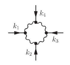
Figure 1: Feynman Diagram corresponding to the fourth cumulant

The expression for the fourth cumulant is given by the connected fourth order correlation in momentum and frequency space as

$$\langle h^{4}(\mathbf{x},t)\rangle_{c} = \int\frac{d^{d+1}\hat{k}_{1}}{(2\pi)^{d+1}}\int\frac{d^{d+1}\hat{k}_{2}}{(2\pi)^{d+1}}\!\int\frac{d^{d+1}\hat{k}_{3}}{(2\pi)^{d+1}}\!\int\frac{d^{d+1}\hat{k}_{4}}{(2\pi)^{d+1}}$$ (13)

$$\langle h(\hat{k}_{1})h(\hat{k}_{2})h(\hat{k}_{3})h(\hat{k}_{4})\rangle_{c}\,e^{i(\hat{k}_{1}+\hat{k}_{2}+\hat{k}_{3}+\hat{k}_{4})\cdot\hat{x}},$$

where $\hat{x}\equiv(\mathbf{x},t)$ and $\hat{k}_{i}\equiv(\mathbf{k}_{i},\omega_{i})$ are vectors in $(d+1)$-vector notation. We use the diagrammatic approach and obtain a connected loop diagram for the fourth cumulant as shown in Fig. 1, where a wiggly line represents the correlation and a solid line the response function. We express the correlation in accordance with the connected loop diagram in Fig. 1, so that

$$\langle h^{4}(\mathbf{x},t)\rangle_{c} = \int\frac{d^{d+1}\hat{k}_{1}}{(2\pi)^{d+1}}\int\frac{d^{d+1}\hat{k}_{2}}{(2\pi)^{d+1}}\!\int\frac{d^{d+1}\hat{k}_{3}}{(2\pi)^{d+1}}\,G(\hat{k}_{1})\,G(\hat{k}_{2})\,G(\hat{k}_{3})$$ (14)

$$L_{4}(\hat{k}_{1},\hat{k}_{2},\hat{k}_{3})\,G(-\hat{k}_{1}-\hat{k}_{2}-\hat{k}_{3}),$$

where $L_{4}$ represents the renormalized loop corresponding to the amputated part of the diagram (excluding the external legs). Its bare value is written as

$$L^{(0)}_{4}(\hat{k}_{1},\hat{k}_{2},\hat{k}_{3}) = 16\left(-\frac{\lambda_{0}}{2}\right)^{4}(2D_{0})^{4}\int\frac{d^{d+1}\hat{q}}{(2\pi)^{d+1}}[\mathbf{q}\cdot(\mathbf{q}-\mathbf{k}_{1})][\mathbf{q}\cdot(\mathbf{k}_{2}+\mathbf{q})]$$ (15)

$$[(\mathbf{q}+\mathbf{k}_{2})\cdot(\mathbf{k}_{3}+\mathbf{k}_{2}+\mathbf{q})][(\mathbf{k}_{4}+\mathbf{k}_{3}+\mathbf{k}_{2}+\mathbf{q})\cdot(\mathbf{q}+\mathbf{k}_{2}+\mathbf{k}_{3})]$$

$$G_{0}(\hat{q})G_{0}(-\hat{q}+\hat{k}_{1})G_{0}(-\hat{q})G_{0}(\hat{q}+\hat{k}_{2})G_{0}(-\hat{q}-\hat{k}_{2})G_{0}(\hat{q}+\hat{k}_{3}+\hat{k}_{2})$$

$$G_{0}(\hat{q}+\hat{k}_{2}+\hat{k}_{3}+\hat{k}_{4})G_{0}(-\hat{q}-\hat{k}_{2}-\hat{k}_{3}),$$

where the prefactor 16 is a combinatorial factor.

Now we evaluate Eq. 15 by performing frequency and momentum integrations where the momentum is restricted to the shell $\Lambda_{0}e^{-r}\leq q\leq\Lambda_{0}$. This leads to

$$L^{<}_{4}(r)=\frac{5}{2}K_{d}\frac{\lambda_{0}^{4}D^{4}_{0}}{\nu_{0}^{7}\Lambda_{0}^{5}}\left(\frac{e^{5r}-1}{5}\right),$$ (16)

where $K_{d}=\frac{S_{d}}{(2\pi)^{d}}$, with $S_{d}$ the surface area of a unit sphere in $d$ dimensional space.

We follow Yakhot and Orszag’s [47, 48] scheme of renormalization without rescaling and obtain from Eq. 16 the differential equation

$$\frac{dL_{4}}{dr}=\frac{5}{2\pi}\frac{\lambda_{0}^{4}D^{4}(r)}{\nu^{7}(r)\Lambda^{5}(r)},$$ (17)

in one dimension.

Noting that $\Lambda(r)=\Lambda_{0}e^{-r}$ and using the asymptotic expressions

$$\nu(r)=\lambda_{0}\sqrt{\frac{D_{0}}{2\pi\nu_{0}\Lambda_{0}}}\,e^{r/2}$$ (18)

and

$$D(r)=\frac{\lambda_{0}D_{0}}{\nu_{0}}\sqrt{\frac{D_{0}}{2\pi\nu_{0}\Lambda_{0}}}\,e^{r/2}$$ (19)

obtained from renormalization-group calculations [49], we obtain the solution to the differential equation (17) as

$$L_{4}(r)=\frac{10\pi}{7}\lambda_{0}\left(\frac{2D^{5}_{0}}{\pi\nu^{5}_{0}\Lambda^{7}_{0}}\right)^{1/2}e^{7r/2}.$$ (20)

The factor $\Lambda_{0}e^{-r}$ is interpreted as a momentum $k_{i}$ in the large scale limit. Since the loop integral must be symmetric with respect to interchange of the external momenta $k_{1}$, $k_{2}$ and $k_{3}$, we replace $\Lambda_{0}e^{-r}$ by the fully symmetric form $k^{1/3}_{1}k^{1/3}_{2}k^{1/3}_{3}$. Thus we have

$$L_{4}(\mathbf{k}_{1},0;\mathbf{k}_{2},0;\mathbf{k}_{3},0)=\frac{10\pi}{7}\lambda_{0}\left(\frac{2D^{5}_{0}}{\pi\nu^{5}_{0}}\right)^{1/2}k^{-7/6}_{1}k^{-7/6}_{2}k^{-7/6}_{3},$$ (21)

when the external frequencies are zero. To obtain the frequency dependency, we take the scaling function as

$$k_{i}^{7/6}f_{4}\left(\frac{\omega_{i}}{k_{i}^{z}}\right)=\frac{1}{k_{i}^{17/6}\nu^{2}(k_{i})|G(\mathbf{k}_{i},\omega_{i})|^{2}},$$ (22)

where the renormalized response function is given by $G(\mathbf{k}_{i},\omega_{i})=[-i\omega_{i}+\nu(k_{i})\mathbf{k}_{i}^{2}]^{-1}$ with the renormalized surface tension

$$\nu(k_{i})=\lambda_{0}\sqrt{\frac{D_{0}}{2\pi\nu_{0}}}\,k_{i}^{-1/2}.$$ (23)

The above scaling relation (22) obeys consistency with the zero frequency limit and with the real valuedness of $\Lambda_{0}e^{-r}$, in addition to being of the correct dimension. Now with the aid of Eq. (22), Eq. (21) is modified to the frequency dependent form

$$L_{4}(\hat{k}_{1},\hat{k}_{2},\hat{k}_{3}) = \frac{10\pi}{7}\lambda_{0}\left(\frac{2D^{5}_{0}}{\pi\nu^{5}_{0}}\right)^{1/2}k_{1}^{17/6}k_{2}^{17/6}k_{3}^{17/6}\,\nu^{2}(k_{1})|G(k_{1},\omega_{1})|^{2}$$ (24)

$$\nu^{2}(k_{2})|G(k_{2},\omega_{2})|^{2}\,\nu^{2}(k_{3})|G(k_{3},\omega_{3})|^{2},$$

representing the renormalized loop diagram in Fig. 1. We substitute the renormalized expression for the loop diagram from Eq. 24 in Eq. 14 and treat the external legs representing the response functions as renormalized. Carring out the frequency integration, we obtain

$$\langle h^{4}(\mathbf{x},t)\rangle_{c}=\frac{10}{7}\left(\frac{D_{0}}{2\pi\nu_{0}}\right)^{2}\int^{\infty}_{-\infty}dk_{1}\int^{\infty}_{-\infty}dk_{2}\!\int^{\infty}_{-\infty}dk_{3}\,\Phi(k_{1},k_{2},k_{3})$$ (25)

where

$$\Phi(k_{1},k_{2},k_{3})=\frac{u(k_{1},k_{2},k_{3})}{v(k_{1},k_{2},k_{3})}$$ (26)

with

$$u(k_{1},k_{2},k_{3}) = (3(|\mathbf{k}_{1}|^{9/2}+|\mathbf{k}_{2}|^{9/2}+|\mathbf{k}_{3}|^{9/2})+5(|\mathbf{k}_{1}|^{3/2}+|\mathbf{k}_{2}|^{3/2}+|\mathbf{k}_{3}|^{3/2})|\mathbf{k}_{1}+\mathbf{k}_{2}+\mathbf{k}_{3}|^{3}$$ (27)

$$+7(|\mathbf{k}_{1}|^{3}+|\mathbf{k}_{2}|^{3}+|\mathbf{k}_{3}|^{3})|\mathbf{k}_{1}+\mathbf{k}_{2}+\mathbf{k}_{3}|^{3/2}+17(|\mathbf{k}_{1}|^{3}|\mathbf{k}_{2}|^{3/2}+|\mathbf{k}_{1}|^{3/2}|\mathbf{k}_{2}|^{3}$$

$$+|\mathbf{k}_{1}|^{3}|\mathbf{k}_{3}|^{3/2}+|\mathbf{k}_{1}|^{3/2}|\mathbf{k}_{3}|^{3}+|\mathbf{k}_{2}|^{3}|\mathbf{k}_{3}|^{3/2}+|\mathbf{k}_{2}|^{3/2}|\mathbf{k}_{3}|^{3})$$

$$+22(|\mathbf{k}_{1}|^{3/2}|\mathbf{k}_{2}|^{3/2}+|\mathbf{k}_{1}|^{3/2}|\mathbf{k}_{3}|^{3/2}+|\mathbf{k}_{2}|^{3/2}|\mathbf{k}_{3}|^{3/2})|\mathbf{k}_{1}+\mathbf{k}_{2}+\mathbf{k}_{3}|^{3/2}$$

$$+90|\mathbf{k}_{1}|^{3/2}|\mathbf{k}_{2}|^{3/2}|\mathbf{k}_{3}|^{3/2}+|\mathbf{k}_{1}+\mathbf{k}_{2}+\mathbf{k}_{3}|^{9/2})$$

and

$$v(k_{1},k_{2},k_{3})=64|\mathbf{k}_{1}|^{7/6}|\mathbf{k}_{2}|^{7/6}|\mathbf{k}_{3}|^{7/6}(|\mathbf{k}_{1}|^{3/2}+|\mathbf{k}_{2}|^{3/2}+|\mathbf{k}_{3}|^{3/2}+|\mathbf{k}_{1}+\mathbf{k}_{2}+\mathbf{k}_{3}|^{3/2})^{4}.$$ (28)

The symmetry of the function $\Phi(k_{1},k_{2},k_{3})$ allows us to write Eq. 25 as

$$\langle h^{4}(\mathbf{x},t)\rangle_{c}=\frac{10}{7}\left(\frac{D_{0}}{2\pi\nu_{0}}\right)^{2}\int^{\infty}_{\mu}dk_{1}\int^{\infty}_{\mu}dk_{2}\!\int^{\infty}_{\mu}dk_{3}\left[2\Phi(k_{1},k_{2},k_{3})+6\Phi(-k_{1},k_{2},k_{3})\right]$$ (29)

where $\mu$ is an infrared cut off. Now we write the integrations separately as

$$I_{1}(\mu)=\int^{\infty}_{\mu}dk_{1}\int^{\infty}_{\mu}dk_{2}\!\int^{\infty}_{\mu}dk_{3}\,\Phi(k_{1},k_{2},k_{3})$$ (30)

and

$$I_{2}(\mu)=\int^{\infty}_{\mu}dk_{1}\int^{\infty}_{\mu}dk_{2}\!\int^{\infty}_{\mu}dk_{3}\,\Phi(-k_{1},k_{2},k_{3}).$$ (31)

These integrals are expected to be of the forms

$$I_{1}(\mu)=a_{1}\mu^{-2}$$ (32)

$$I_{2}(\mu)=a_{2}\mu^{-2}.$$ (33)

where $a_{1}$ and $a_{2}$ are dimensionless constants. Substituting Eqs. 32 and 33 in Eq. 29 yields

$$\langle h^{4}(\mathbf{x},t)\rangle_{c}=\frac{10}{7}[2a_{1}+6a_{2}]\left(\frac{D_{0}}{2\pi\nu_{0}}\right)^{2}\frac{1}{\mu^{2}}$$ (34)

We evaluate the integrals in Eqs. 30 and 31 by integrating over $k_{1}$, $k_{2}$ and $k_{3}$ numerically and obtain the dimensionless constants as

$$a_{1}=\lim_{\mu\rightarrow 0^{+}}[\mu^{2}I_{1}(\mu)]=0.007505$$ (35)

and

$$a_{2}=\lim_{\mu\rightarrow 0^{+}}[\mu^{2}I_{2}(\mu)]=0.026297,$$ (36)

the numerical values having converged to the above values for decreasing values of the parameter $\mu$ very close to zero.

4 The Kurtosis

Having calculated the fourth-order cumulant given by Eq. (34), we now need the value of the second-order cumulant to determine the value of kurtosis given by Eq. (10). The second moment is written as

$$\langle h^{2}(\mathbf{x},t)\rangle=\int\frac{d^{d}k_{1}\,d\omega_{1}}{(2\pi)^{d+1}}\int\frac{d^{d}k_{2}\,d\omega_{2}}{(2\pi)^{d+1}}\,\langle h(\mathbf{k}_{1},\omega_{1})h(\mathbf{k}_{2},\omega_{2})\rangle\,e^{i(\mathbf{k}_{1}+\mathbf{k}_{2})\cdot\mathbf{x}}\,e^{-i(\omega_{1}+\omega_{2})t}.$$ (37)

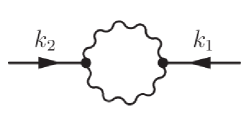
Figure 2: Feynman diagram corresponding to the second moment

Homogeneity in space and time implies that the correlation takes the form

$$\langle h(\mathbf{k}_{1},\omega_{1})\,h(\mathbf{k}_{2},\omega_{2})\rangle=Q(\mathbf{k}_{1},\omega_{1})\,(2\pi)^{d}\delta^{d}(\mathbf{k}_{1}+\mathbf{k}_{2})\,(2\pi)\delta(\omega_{1}+\omega_{2}).$$ (38)

The correlation function $Q(\mathbf{k},\omega)$ can be written in accordance with the one-loop diagram in Fig. 2, so that

$$\langle h^{2}(\mathbf{x},t)\rangle_{c}=\langle h^{2}(\mathbf{x},t)\rangle=\int\frac{d^{d}k\,d\omega}{(2\pi)^{d+1}}\,G(\mathbf{k},\omega)\,L_{2}(\mathbf{k},\omega)\,G(-\mathbf{k},-\omega)$$ (39)

The renormalized value of $L_{2}$, given by the loop integral coming from the amputated part of Fig. 2, can be obtained as

$$L_{2}(\mathbf{k},\omega)=\frac{\lambda^{2}_{0}D^{2}_{0}}{\pi\nu^{2}_{0}}\,k\,|G(\mathbf{k},\omega)|,$$ (40)

by means of a renormalization scheme as shown in Ref. [49]. This yields the second cumulant as

$$\langle h^{2}(\mathbf{x},t)\rangle_{c}=\frac{4}{\pi}\left(\frac{D_{0}}{2\pi\nu_{0}}\right)\frac{1}{\mu}.$$ (41)

Employing Eqs. (25) and (41) in the definition of kurtosis leads to

$$Q=\frac{\langle h^{4}(\mathbf{x},t)\rangle_{c}}{\langle h^{2}(\mathbf{x},t)\rangle^{2}_{c}}=\frac{5\pi^{2}}{28}(a_{1}+3a_{2}),$$ (42)

free from the infra-red cutoff $\mu$ and the model parameters $\nu_{0}$, $D_{0}$, and $\lambda_{0}$. Employing the numerical values of $a_{1}$ and $a_{2}$ from Eqs. 35 and 36 yields the kurtosis as

$$Q=0.152267.$$ (43)

We compare this value with other stationary values of kurtosis in Table 1.

Table 1: Values of Kurtosis in $(1+1)$ dimensions.

System of study	Method	Kurtosis	Reference
PNG (stationary)	Numerical	$0.289$	[21]
g1 DPRM (stationary)	Numerical	$0.278$	[50]
KPZ (present calculation)	Analytical	$0.1523$	Eq. (43)

5 Discussion and Conclusion

In this work, we followed a perturbative renormalization approach to evaluate the Feynman diagram in Fig. 1 that represents the fourth cumulant, noting that contribution to cumulants are given by the connected loop diagrams. To calculate the connected diagram, we first renormalized its amputated part in the limit of internal momenta and frequencies much greater than the external ones and followed Yakhot and Orszag’s iterative renormalization scheme without rescaling [48]. This results in a scale dependent function for the amputated part of the loop diagram at zero frequency. Introducing a frequency dependent scaling function that smoothly joins with the obtained scaling behavior and that preserves the property of real valuedness, we evaluated the resulting frequency and momentum integrations to obtain an expression for the fourth order cumulant depending on the infrared cutoff in the momentum integration. The evaluation of the second cumulant is simpler which also depends on the the infrared cutoff as shown in Ref. [49]. The behaviors of both the fourth and second order cumulants are seen to be exactly in accordance with the well-known behavior of the $n$th moment, namely $W_{n}\sim L^{n\chi}$, where $L$ is the substrate size (so that $\mu\sim L^{-1}$) and $\chi$ is the roughness exponent. These cumulants yield the value of kurtosis $Q=0.1523$ which is free from the infrared cutoff $\mu$ and model dependent parameters $D_{0}$ , $\nu_{0}$, and $\lambda_{0}$, due to their exact cancellations.

Incidentally, it may be worth mentioning that the calculation of cumulant amplitudes have been regarded as an important objective by some researchers. For example, Krug et al. [27] studied the growth of an interface via simulation of the single step model with flat initial condition and obtained the estimates for the cumulant amplitudes as $c_{2}=0.404\pm 0.013$ and $c_{4}=0.020\pm 0.002$, suggesting a kurtosis value $Q=\frac{c_{4}}{c_{2}^{2}}=0.123\pm 0.020$. Furthermore, they showed that $c_{2}$ is higher for the steady state case, namely, $c_{2}=0.712\pm 0.003$, due to the additional role of fluctuations in the initial conditions besides those operating during the growth. Earlier, Hwa and Frey [51] had obtained $c_{2}=0.69$ via mode-coupling calculations. Tang [52] estimated $c_{2}=0.725\pm 0.005$ using a Monte-Carlo simulation with the single-step model, giving an excellent estimate for the Baik-Rains constant [21, 53]. A slightly different result, $c_{2}=0.71$, was obtained through mode-coupling calculation by Amar and Family [54].

In Table 1, our calculated kurtosis value is compared with other stationary values. Prähofer and Spohn [21] studied the PNG model belonging to the $1+1$ dimensional KPZ universality class to find the effect of initial conditions on the statistical behavior of growing interfaces. They obtained different kurtosis values for different initial conditions, namely, $Q=0.0934$ for curved, $Q=0.1652$ for flat, and $Q=0.289$ for stationary initial conditions. Halpin-Healy and Lin [50] studied the DPRM with different configurations such as point-to-point, point-to-line, and stationary cases, leading to GUE-TW, GOE-TW and Baik-Rains $F_{0}$ distributions, respectively. Through $g_{1}$ DPRM, they estimated the stationary kurtosis value to be $Q=0.278$.

Apart from the values shown in Table 1, there are a few studies where the full Baik-Rains distribution is obtained in the context of KPZ stationary state. Takeuchi [42] obtained, via a numerical simulation of the PNG model and an experiment on the TLC, a universal function that undergoes a crossover from a transient state to the stationary regime. Miettinen et al. [23] carried out an experimental study of the slow propagation of the combustion front on a sheet of paper to investigate upon the front fluctuation distribution. Their experimental data for the transient and stationary states were found to fit well with the GOE-TW and $F_{0}$ distributions, respectively. On the other hand, Halpin-Healy and Lin [50], studied the distributions of deposition models (BD, SSM, and RSOS) that strongly agree with DPRM/SHE results and they turn out to be the Baik-Rains distribution. These investigations establish that the kurtosis value in the stationary state must be the same as the universal kurtosis of the Baik-Rains distribution (for example, $Q=0.289$ [21] or $0.278$ [50]).

In our calculation based on the RG scale elimination scheme, we obtained the renormalized quantities in the large-scale and long-time limits. Thus our methodology inexorably selects the stationary regime. However, the resulting kurtosis value does not agree well with the stationary kurtosis value and it is distinctly lower than the Baik-Rains value, $Q=0.28916$. In our simplified scheme of calculation, we obtained the fourth cumulant at one-loop order. While a one-loop scheme for the third cumulant was nearly successful in estimating the stationary skewness value [49], a higher order calculation would appear to be more appropriate for the fourth cumulant. Noting that the perturbation expansion is about a Gaussian state, the Gaussian behavior seems to play some role with the increase in order of the cumulant, lowering the estimated value. This opens the door for further investigations into the rather unexplored stationary KPZ problem that is expected to illuminate upon its semantic relation with Baik-Rains distribution.

We conclude by recalling that there are many growth processes governed by nonequilibrium dynamics that are believed to be in the KPZ universality class on the basis of scaling exponents. However, as shown by the PNG and TLC studies, the statistical behavior, that is the probability distribution, depends on the initial conditions. The full probability distribution function of the KPZ height fluctuations has never been studied analytically due to the inherent difficulty in the problem. However, relevant information about the probability distribution can be obtained through the study a few higher order moments and cumulants. Thus the present theoretical study may be viewed as an initial attempt at the quantification of higher order statistical property of the $1+1$ dimensional KPZ dynamics. We hope that such analytical scheme would be useful for the study of statistical behavior of other important stochastic processes as well.

Acknowledgements

We thank M. Prähofer and H. Spohn for making their data available online [55]. T. Singha thanks the MHRD, Government of India, for financial support through a scholarship.

References

References

- [1] A.-L. Barabási and H. E. Stanley, Fractal Concepts in Surface Growth (Cambridge University Press, Cambridge, 1995).
- [2] J. Krug, Adv. Phys. 46, 139 (1997).
- [3] T. Halpin-Healy and Y.-C. Zhang, Phys. Rep. 254, 215 (1995).
- [4] P. Meakin, Phys. Rep. 235, 189 (1993).
- [5] F. Family and T. Vicsek, J. Phys. A 18, L75 (1985).
- [6] M. Kardar, G. Parisi, and Y.-C. Zhang, Phys. Rev. Lett. 56, 889 (1986).
- [7] P. Pfeifer, D. Avnir, and D. Farin, Surf. Sci. 126, 569 (1983).
- [8] M. Moskovits, Rev. Mod. Phys. 57, 783 (1985).
- [9] P. Meakin, P. Ramanlal, L. M. Sander, and R. C. Ball, Phys. Rev. A 34, 5091 (1986).
- [10] J. Krug, Phys. Rev. A 36, 5465 (1987).
- [11] E. Medina, T. Hwa, M. Kardar, and Y.-C. Zhang, Phys. Rev. A 39, 3053 (1989).
- [12] T. Paiva and F. Aarão Reis, Surf. Sci. 601, 419 (2007).
- [13] T. Vicsek, M. Cserzõ, and V. K. Horváth, Physica A 167, 315 (1990).
- [14] M. A. C. Huergo, M. A. Pasquale, A. E. Bolzán, A. J. Arvia, and P. H. González, Phys. Rev. E 82, 031903 (2010).
- [15] M. A. Rubio, C. A. Edwards, A. Dougherty, and J. Gollub, Phys. Rev. Lett. 63, 1685 (1989).
- [16] K. A. Takeuchi and M. Sano, Phys. Rev. Lett. 104, 230601 (2010).
- [17] K. A. Takeuchi, M. Sano, T. Sasamoto, and H. Spohn, Sci. Rep. 1, 34 (2011).
- [18] W. van Saarloos and G. H. Gilmer, Phys. Rev. B 33, 4927 (1986).
- [19] N. Goldenfeld, J. Phys. A 17, 2807 (1984).
- [20] J. Krug and H. Spohn, Phys. Rev. A 38, 4271 (1988).
- [21] M. Prähofer and H. Spohn, Phys. Rev. Lett. 84, 4882 (2000).
- [22] M. Myllys, J. Maunuksela, M. Alava, T. Ala-Nissila, J. Merikoski, and J. Timonen, Phys. Rev. E 64, 036101 (2001).
- [23] L. Miettinen, M. Myllys, J. Merikoski, and J. Timonen, Eur. Phys. J. B 46, 55 (2005).
- [24] D. Forster, D. R. Nelson, and M. J. Stephen, Phys. Rev. A 16, 732 (1977).
- [25] M. Kardar and Y.-C. Zhang, Phys. Rev. Lett. 58, 2087 (1987).
- [26] D. S. Fisher and D. A. Huse, Phys. Rev. B 43, 10728 (1991).
- [27] J. Krug, P. Meakin, and T. Halpin-Healy, Phys. Rev. A 45, 638 (1992).
- [28] T. Hwa and M. Lässig, Phys. Rev. Lett. 76, 2591 (1996).
- [29] T. Hwa, Nature (London) 399 (1999).
- [30] M. Eden, in Proceedings of the Fourth Berkeley Symposium on Mathematical and Statistics and Probability , edited by F. Neyman (Berkeley and Los Angeles: University of California Press, 1961).
- [31] M. Plischke and Z. Rácz, Phys. Rev. Lett. 53, 415 (1984).
- [32] R. Jullien and R. Botet, Phys. Rev. Lett. 54, 2055 (1985).
- [33] M. Plischke and Z. Rácz, Phys. Rev. A 32, 3825 (1985).
- [34] M. Plischke, Z. Rácz, and D. Liu, Phys. Rev. B 35, 3485 (1987).
- [35] F. Colaiori and M. A. Moore, Phys. Rev. Lett. 86, 3946 (2001).
- [36] H. van Beijeren, R. Kutner, and H. Spohn, Phys. Rev. Lett. 54, 2026 (1985).
- [37] M. Lässig, Phys. Rev. Lett. 80, 2366 (1998).
- [38] M. Schwartz and S. F. Edwards, Europhys. Lett. 20, 301 (1992).
- [39] L. Canet, H. Chaté, B. Delamotte, and N. Wschebor, Phys. Rev. Lett. 104, 150601 (2010).
- [40] T. Kloss, L. Canet, and N. Wschebor, Phys. Rev. E 86, 051124 (2012).
- [41] T. Imamura and T. Sasamoto, Phys. Rev. Lett. 108, 190603 (2012).
- [42] K. A. Takeuchi, Phys. Rev. Lett. 110, 210604 (2013).
- [43] Y. Shim and D. P. Landau, Phys. Rev. E 64, 036110 (2001).
- [44] D. A. Huse, C. L. Henley, and D. S. Fisher, Phys. Rev. Lett. 55, 2924 (1985).
- [45] G. Parisi, J. Phys. France 51, 1595 (1990).
- [46] F. D. A. Aarão Reis, Phys. Rev. E 70, 031607 (2004).
- [47] V. Yakhot and S. A. Orszag, Phys. Rev. Lett. 57, 1722 (1986).
- [48] V. Yakhot and S. A. Orszag, J. Sci. Comput. 1, 3 (1986).
- [49] T. Singha and M. K. Nandy, Phys. Rev. E 90, 062402 (2014).
- [50] T. Halpin-Healy and Y. Lin, Phys. Rev. E 89, 010103 (2014).
- [51] T. Hwa and E. Frey, Phys. Rev. A 44, R7873 (1991).
- [52] L.-H. Tang, J. Stat. Phys. 67, 819 (1992).
- [53] T. Halpin-Healy, Phys. Rev. E 88, 042118 (2013).
- [54] J. G. Amar and F. Family, Phys. Rev. A 45, 5378 (1992).
- [55] M. Prähofer and H. Spohn, http://www-m5.ma.tum.de/KPZ