Skewness in (1+1)-dimensional Kardar-Parisi-Zhang type Growth

Abstract

We use the $(1+1)$-dimensional Kardar-Parisi-Zhang equation driven by a Gaussian white noise and employ the dynamic renormalization-group of Yakhot and Orszag without rescaling [J. Sci. Comput. 1, 3 (1986)]. Hence we calculate the second and third order moments of height distribution using the diagrammatic method in the large scale and long time limits. The moments so calculated lead to the value $S=0.3237$ for the skewness. This value is comparable with numerical and experimental estimates.

I Introduction

The study of surface growth has been one of the most important problems in non-equilibrium statistical physics over the past few decades book_stanley ; krug97 ; Halpin95 ; Meakin93 ; Family_Physica . The most generic continuum model of surface growth is the Kardar-Parisi-Zhang (KPZ) equation that is endowed with interesting properties of statistical scale invariance. Kardar, Parisi and Zhang KPZ86 suggested a nonlinear differential equation for local surface growth in the form

$$\frac{\partial h(\mathbf{x},t)}{\partial t}=\nu_{0}\nabla^{2}h+\frac{\lambda_{0}}{2}(\nabla h)^{2}+\eta(\mathbf{x},t),$$ (1)

where $h(\mathbf{x},t)$ is the height of the surface at position $\mathbf{x}$ and time $t$ on a $d$ dimensional substrate, $\nu_{0}$ is the surface tension that has a tendency to make the surface smooth, and the coupling constant $\lambda_{0}$ measures the strength of the nonlinear interaction term. The nonlinear term induces local growth along the normal to the surface and gives rise to lateral correlations. On the other hand, the linear term (containing $\nu_{0}$) is responsible for diffusion of particles to the local minima VLDS_91 . The driving term $\eta(\mathbf{x},t)$, describing the random deposition of particles, is assumed to obey a Gaussian distribution to account for the stochastic nature of the flux of particles. It is taken to be a Gaussian white noise with zero mean, $\langle\eta(\mathbf{x},t)\rangle=0$, and with correlation

$$\langle\eta(\mathbf{x},t)\,\eta(\mathbf{x}^{\prime},t^{\prime})\rangle=2D_{0}\,\delta^{d}(\mathbf{x}-\mathbf{x}^{\prime})\,\delta(t-t^{\prime}),$$ (2)

where $D_{0}$ is a constant and the angular brackets denote ensemble averages.

There are many deposition models that have been identified with the KPZ universality class. A few examples are the ballistic deposition Meakin86 ; Family_Physica , the Eden model plischke_prl_84 ; jullien_85 ; eden_plischke_85 , the restricted solid-on-solid (RSOS) model Meakin93 , and the single step model (SSM) Meakin86 ; Plischek_87 . A large number of growth experiments show scaling exponents close to those of the KPZ growth problem. A few important phenomena are thin film growth book_stanley , bacterial colony growth jullien_85 ; Vicsek_90 , growth of fractals Family_Vicsek91 , turbulent liquid crystal (TLC) growth K_A_Takeuchi ; kazumasa , and one dimensional polynuclear growth (PNG) saarloos_86 ; goldenfeld ; krug_pra_88 ; Michael_Herbert_00 , etc. Apart from such growth models, the KPZ problem is related to various other processes such as the noisy Burgers equation forster_pra_16_732_77 , flame front propagation kuramoto2003chemical ; sivashinsky_Acta_77 , directed polymer in random media KPZ86 ; fisher91 ; kpz87 ; JMKIM ; Halpin95 , interface roughening due to impurities huse_85 ; huse85 , and growing interfaces in randomly stirred fluids kerstein_92 . A great amount of work has been carried out, mostly via numerical and experimental studies, in various KPZ type surface growth problems. The interplay of non-linearity, surface tension, and uncorrelated noise in such problems establish a universality class distinct from that of the Edward-Wilkinson type growth in the large-scale long-time limit. The mean-square of the height fluctuations is related to the critical exponents KPZ89 as

$$\langle[h(\mathbf{x},t)-h(\mathbf{x}^{\prime},t^{\prime})]^{2}\rangle\sim|\mathbf{x}-\mathbf{x}^{\prime}|^{2\chi}\,\,\psi\left(\frac{|t-t^{\prime}|}{|\mathbf{x}-\mathbf{x}^{\prime}|^{z}}\right),$$ (3)

where $\chi$ is the roughness exponent describing the self-affine geometry of the surface, $z$ is the dynamic exponent (the ratio $\frac{\chi}{z}=\beta$ is the growth exponent), and $\psi(\cdot)$ is a scaling function. The roughness exponent $\chi$ is an important parameter Baiod88 in the studies of adsorption, catalysis Pfeifer_83 , and optical properties Moskovits_85 of a thin film. The properties of a rough surface are determined by the distribution of height fluctuations and it deserves attention both in theoretical and experimental studies of growing interfaces Meakin93 .

Various analytical approaches have been employed to study the universality class of the KPZ equation on the basis of scaling exponents in different dimensions. The dynamic renormalization-group by Kardar, Parisi, and Zhang KPZ86 leads to the values of roughness exponent $\chi=\frac{1}{2}$ and dynamic exponent $z=\frac{3}{2}$ at one-loop order for the $(1+1)$ dimensional KPZ equation. Motivations in the theoretical study of the KPZ equation in higher dimensions have led to formulations of different analytical techniques. Examples of such theoretical studies are the mode coupling scheme Colaiori_PRL_86_3946 ; Beijeren_PRL_54_2026 ; Hwa_PRA_44_R7873 , the operator product expansion Lassig_PRL_80_2366 , the self-consistent expansion Schwartz_Edwards_1992 and a nonperturbative renormalization group Canet_PRL_104_150601 ; Kloss_PRE2012 for the calculation of scaling exponents in the strong coupling regime.

These exponents have also been computed numerically considering different growth rules. Apart from the numerical studies, many experiments have been carried out to find these exponents. Various experimental studies kazumasa ; Huergo_radial ; Huergo_10 have indicated that the roughness exponent is about $0.50$ and the growth exponent $0.33$ which have been identified with the universality class of the $(1+1)$ dimensional KPZ type surface growth.

Besides the critical exponents, the probability distribution function is an important feature to classify the universality of a physical process JMKIM . In experiments, measurements of normalized moments is expected to be more accurate than the measurement of scaling exponents Meakin93 . Thus higher order moments can infer about the universality class in a better way than the critical exponents Reis_pre_70_031603_05 . Consequently, higher order moments are very important in the study of surface morphology and the universality class can be better realized through the values of higher order moments and a parameter such as skewness.

The skewness has been computed numerically employing a variety of deposition algorithms. Krug et al. J-krug_92 , using the simulation in a single step model for flat initial condition, obtained $|S|=0.28\pm 0.04$ in the transient regime. Following the same model, they prepared stationary interfaces by taking uncorrelated spins ($\sigma_{i}=\pm 1$) and obtained $|S|\approx 0.33$. Prähofer and Spohn Michael_Herbert_00 took the polynuclear growth model and mapped it into a random permutation through the droplet geometry thereby onto Gaussian random matrices to understand the dependence of the initial conditions on height fluctuations. They inferred that the droplet and flat substrates have the same scaling form but distinct universal distributions. They estimated the skewness for three different shapes, namely, curved, flat, and stationary self-similar in $(1+1)$ dimensions. For the flat shape, they obtained $S=0.2935$, for the curved shape, $S=0.2241$, and for the stationary self-similar case, $S=0.35941$. They proposed an expression for the height distribution, namely $h(\mathbf{x},t)\simeq v_{\infty}t+(\Gamma t)^{1/3}\zeta$ with $\zeta$ a random variable, where $\Gamma=\frac{D_{0}^{2}\lambda_{0}}{8\nu_{0}^{2}}$ is a model parameter and $v_{\infty}$ is the growth rate in the asymptotic limit K_A_Takeuchi . It was found that $\zeta$ obeys the Tracy-Widom (TW) distribution corresponding to the largest eigenvalues of random matrices kazumasa . For curved interfaces the random matrices form a Gaussian unitary ensemble (GUE) sasamoto_prl_104_230602_10 whereas for flat interfaces they form a Gaussian orthogonal ensemble (GOE).

In an experiment on growing interfaces in liquid crystal turbulence, Takeuchi et al. kazumasa ; K_A_Takeuchi found that the growth and roughness exponents are the same as those of the KPZ type growth in one dimension in the asymptotic limit. Their experimental data indicated the value for skewness $S\simeq 0.29$ for a flat interface, whereas for a curved interface their experimental data converged to $S=0.2241$. They concluded that the probability distribution function (pdf) of interface fluctuations precisely agrees with the GOE of TW distribution for the flat interface, whereas the curved interface fluctuations agree with the GUE of TW distribution, up to fourth order cumulants. Sasamoto and Spohn sasamoto_prl_104_230602_10 ; 2010JSMTE_11_013S solved the $(1+1)$ dimensional KPZ problem with an initial condition of curved-height profile and showed that the pdf follows the GUE of TW distribution of random matrices.

It may be noted that there have been very few analytical evaluations of the skewness and higher order moments for the KPZ type growth problem. The one known to the authors is a mean field calculation yielding $S=\pm 0.46$ in $(1+1)$ dimensions meanfield with the flat initial condition $h(x,0)=0$ for the transient regime.

In this work, we are interested in the KPZ growth problem for a flat interface and seek to calculate the skewness of height fluctuations in the stationary state. Consequently, we apply the dynamic renormalization group scheme without rescaling to the KPZ equation. This scheme was previously employed by Yakhot and Orszag yakhot_j_s_comput_1_3_86 to calculate various universal numbers in the case of hydrodynamic turbulence. This scheme enables us to calculate the second and third order moments of height fluctuations in a straightforward manner. The ensuing result for skewness is compared with the findings of various numerical, experimental, and theoretical studies in Table 1.

The paper is organized as follows. In Section 2, the renormalizaiton-group scheme without rescaling is applied to the KPZ problem. Section 3 outlines the definition of statistical moments of height fluctuations and presents calculations of the second and third order statistical moments. Finally, Section 4 presents a discussion and conclusion and a comparison with other findings.

II Renormalization Scheme without Rescaling

The nonlinear dynamics described by the KPZ equation (1) incorporates interaction among many degrees of freedom KPZ89 . The complexity of such interactions among the collective set of height fluctuations is most easily seen when we Fourier transform the height fluctuations $h(\mathbf{x},t)$ and the driving field $\eta(\mathbf{x},t)$. The Fourier space is also suitable for employing the dynamic renormalization-group techniques hohenberg_rmp_49_435_77 . The Fourier transform of the height fluctuations $h(\mathbf{x},t)$ is expressed as

$$h(\mathbf{x},t)=\int\frac{d^{d}k\,d\omega}{(2\pi)^{d+1}}\,h(\mathbf{k},\omega)\,e^{i(\mathbf{k}\cdot\mathbf{x}-\omega t)},$$ (4)

where $d$ is the substrate dimension. The stochastic noise $\eta(\mathbf{x},t)$ is also Fourier transformed in a similar manner. The Fourier amplitude of the noise fluctuations has a zero mean, $\langle\eta(\mathbf{k},\omega)\rangle=0$, and the noise-correlation can be expressed as

$$\langle\eta(\mathbf{k},\omega)\,\eta(\mathbf{k}^{\prime},\omega^{\prime})\rangle=2D_{0}\,(2\pi)^{d}\delta^{d}(\mathbf{k}+\mathbf{k}^{\prime})\,2\pi\delta(\omega+\omega^{\prime}),$$ (5)

in the Fourier space, as a consequence of Eq. 2. Using Eq. (4), the Fourier transform of the KPZ equation [Eq. (1)] is obtained as

$$(-i\omega+\nu_{0}k^{2})\,h(\mathbf{k},\omega)=\eta(\mathbf{k},\omega)-\frac{\lambda_{0}}{2}\int\!\!\int\frac{d^{d}q\,d\Omega}{(2\pi)^{d+1}}\,[\mathbf{q}\cdot(\mathbf{k}-\mathbf{q})]\,h(\mathbf{q},\Omega)\,h(\mathbf{k}-\mathbf{q},\omega-\Omega).$$ (6)

which is in a form particularly useful for implementing the renormalization-group scheme.

II.1 Scale Elimination

To implement the renormalization-group scheme, we eliminate height fluctuations $h^{>}(\mathbf{q},\Omega)$ belonging to the shell $\Lambda_{0}e^{-r}\leq q\leq\Lambda_{0}$ in the wavevector space by substituting for $h^{>}(\mathbf{q},\Omega)$ in the equation for $h^{<}(\mathbf{k},\omega)$ following from Eq. (6). This process generates a perturbation series in powers of the coupling constant $\lambda_{0}$. Considering terms up to second order in $\lambda_{0}$ yields the equation

$$[-i\omega+\nu_{0}k^{2}+\Sigma(\mathbf{k},\omega)]\,h^{<}(\mathbf{k},\omega)=\eta^{<}(\mathbf{k},\omega)$$ (7)

$$-\frac{\lambda_{0}}{2}\int\!\!\int\frac{d^{d}q\,d\Omega}{(2\pi)^{d+1}}\,[\mathbf{q}\cdot(\mathbf{k}-\mathbf{q})]\,h^{<}(\mathbf{q},\Omega)\,h^{<}(\mathbf{k}-\mathbf{q},\omega-\Omega).$$

in the range $0\leq k\leq\Lambda_{0}e^{-r}$ in the wavevector space, where $\Sigma(\mathbf{k},\omega)$ is the self energy correction represented by the amputated part of the Feynman diagram shown in Fig. 1.

Figure 1: Self-energy correction. The self-energy $\Sigma(\mathbf{k},\omega)$ corresponds to the loop. Propagators are indicated by arrowed lines and correlation by a wiggly line.

The corresponding loop integral is given by

$$\Sigma(\mathbf{k},\omega)=4\left(-\frac{\lambda_{0}}{2}\right)^{2}\int\frac{d^{d}q}{(2\pi)^{d}}\,(\mathbf{k}\cdot\mathbf{q})\,[\mathbf{q}\cdot(\mathbf{k}-\mathbf{q})]\int^{\infty}_{-\infty}\frac{d\Omega}{2\pi}\,|G^{>}_{0}(\hat{q})|^{2}\,(2D_{0})\,G^{>}_{0}(\hat{k}-\hat{q}),$$ (8)

where $G_{0}(\hat{k})\equiv G_{0}(\mathbf{k},\omega)=[-i\omega+\nu_{0}k^{2}]^{-1}$ is the bare propagator and the prefactor 4 is a combinatorial factor. Following Refs. KPZ89 ; yakhot_j_s_comput_1_3_86 , we symmetrize the internal momenta by taking the transformation $\mathbf{q}\rightarrow(\mathbf{q}+\mathbf{k}/2)$. Performing the frequency convolution and evaluating the integral over the internal momenta in the shell $\Lambda_{0}e^{-r}\leq q\leq\Lambda_{0}$ yields the self energy

$$\Sigma(k,0)=\frac{\lambda_{0}^{2}D_{0}}{2\nu_{0}^{2}\Lambda_{0}^{2-d}}\frac{S_{d}}{(2\pi)^{d}}\left(\frac{2-d}{2d}\right)\frac{e^{(2-d)r}-1}{2-d}\,k^{2}$$ (9)

in the large scale ($k\rightarrow 0$) and long time ($\omega\rightarrow 0$) limits, where $S_{d}=\frac{2\pi^{d/2}}{\Gamma(d/2)}$ is the surface area of a sphere of unit radius embedded in a $d$ dimensional space. As a result of the above elimination, the effective surface tension is obtained as

$$\nu^{<}(r)=\nu_{0}\left[1+\frac{1}{4}K_{d}\frac{\lambda^{2}_{0}D_{0}}{\nu^{3}_{0}\Lambda^{2-d}_{0}}\frac{e^{(2-d)r}-1}{d}\right],$$ (10)

where $K_{d}=\frac{S_{d}}{(2\pi)^{d}}$ and the second term in the parentheses comes from the self energy correction.

The height-height correlation is also expanded in a perturbative series in a similar manner. This gives rise to a correction to the noise amplitude, given by

$$2D^{<}(r)=2D_{0}+2\left(\frac{-\lambda_{0}}{2}\right)^{2}\int\frac{d^{d}q}{(2\pi)^{d}}\,[\mathbf{q}\cdot(\mathbf{k}-\mathbf{q})]^{2}\int^{\infty}_{-\infty}\frac{d\Omega}{2\pi}\,|G^{>}_{0}(\hat{q})|^{2}\,(2D_{0})^{2}\,|G^{>}_{0}(\hat{k}-\hat{q})|^{2},$$ (11)

where $D^{<}(r)$ is the effective amplitude of noise correlation, whereas $D_{0}$ is the bare parameter appearing in the noise correlation in Eq. (5). The corresponding equation is shown diagrammatically in Fig. 2.

Figure 2: Perturbation expansion of the correlation $Q(\mathbf{k},\omega)$ to one-loop order.

Calculating the loop integral in the large scale and long time limits, $k\rightarrow 0$ and $\omega\rightarrow 0$, the correction to the noise amplitude is obtained as

$$\Delta D=D_{0}\frac{\lambda_{0}^{2}D^{2}_{0}}{4\nu_{0}^{3}\Lambda^{2-d}_{0}}\frac{S_{d}}{(2\pi)^{d}}\frac{e^{(2-d)r}-1}{2-d}.$$ (12)

Thus the effective amplitude of the noise correlation is given by

$$D^{<}(r)=D_{0}\left[1+\frac{1}{4}K_{d}\frac{\lambda_{0}^{2}D_{0}}{\nu_{0}^{3}\Lambda^{2-d}_{0}}\frac{e^{(2-d)r}-1}{2-d}\right].$$ (13)

We observe that the surface tension $\nu_{0}$ and noise amplitude $D_{0}$ acquire corrections due to the elimination of small scales belonging to the high-momentum shell $\Lambda_{0}e^{-r}\leq k\leq\Lambda_{0}$.

II.2 Flow Equations and Fixed Point

To implement the renormalization scheme, we shall follow a procedure suggested by Yakhot and Orszag yakhot_j_s_comput_1_3_86 ; yakhot_prl_57_1772_86 where the renormalized parameters are not rescaled after the above scale elimination operation. A particular advantage with this scheme is that the flow equations for the renormalized parameters are obtained directly with respect to the elimination parameter $r$. Implementing this scheme, we obtain, from Eqs. 10 and 13, the flow equations for the renormalized surface tension $\nu(r)$ and renormalized noise amplitude $D(r)$ as the differential equations

$$\frac{d\nu}{dr}=\frac{1}{4}K_{d}\left(\frac{2-d}{d}\right)\frac{\lambda_{0}^{2}D(r)}{\nu^{2}(r)\Lambda^{2-d}(r)}$$ (14)

and

$$\frac{dD}{dr}=\frac{1}{4}K_{d}\frac{\lambda_{0}^{2}D^{2}(r)}{\nu^{3}(r)\Lambda^{2-d}(r)},$$ (15)

where $\Lambda(r)=\Lambda_{0}e^{-r}.$ In this scheme, there is no flow equation for the coupling constant $\lambda_{0}$ as it does not acquire any correction due to Galilean invariance. In order to find the fixed point, we define an effective coupling, $g(r)$, as

$$g(r)=K_{d}\frac{\lambda_{0}^{2}D(r)}{\nu^{3}(r)\Lambda^{2-d}(r)}.$$ (16)

Using Eqs. 14 and 15, the flow equation for this effective coupling is obtained as

$$\frac{dg}{dr}=a\,g(r)-b\,g^{2}(r),$$ (17)

where $a=2-d$, and $b=\frac{3-2d}{2d}$. Integrating this equation, we obtain an $r$-dependent expression for the effective coupling, given by

$$g(r)=\frac{g_{0}e^{ar}}{1+\frac{b}{a}g_{0}(e^{ar}-1)},$$ (18)

where $g_{0}=g(0)=K_{d}\frac{\lambda^{2}_{0}D_{0}}{\nu^{3}_{0}\Lambda^{2-d}_{0}}$. The fixed point value $g^{*}$ is obtained in the limit $r\rightarrow\infty$. For $d\leq 2$, we get

$$g^{*}=\frac{a}{b}=\frac{2d(2-d)}{(3-2d)}.$$ (19)

We see that the fixed point value $g^{*}$ diverges for the substrate dimension $d=1.5$ and it is finite and positive in the range $0\leq d<1.5$. However, in the range $1.5<d<2$, the coupling constant is finite but negative, and it vanishes at $d=2$. These fixed point values are consistent with Frey and Täuber’s one-loop calculation (frey_pre_50_1024_94, , Cf. Eq. (3.18)). In this paper, we are interested in the substrate dimension $d=1$; thus the effective coupling constant approaches the fixed point value $g^{*}=2$.

Using Eqs. (16) and (18), the differential equations (14) and (15) yield the exact solutions

$$\nu(r)=\nu_{0}\left[1+\frac{bg_{0}}{a}(e^{ar}-1)\right]^{a/4bd}$$ (20)

and

$$D(r)=D_{0}\left[1+\frac{bg_{0}}{a}(e^{ar}-1)\right]^{1/4b}.$$ (21)

For very large $r$, the above solutions lead to the asymptotic expressions

$$\nu(r)\simeq\nu_{0}\left(\frac{bg_{0}}{a}e^{ar}\right)^{a/4bd}$$ (22)

and

$$D(r)\simeq D_{0}\left(\frac{bg_{0}}{a}e^{ar}\right)^{1/4b}.$$ (23)

in the large scale limit. Noting that $a=1$ and $b=\frac{1}{2}$ for our case $d=1$, these expressions for surface tension and noise amplitude reduce to

$$\nu(r)\simeq\nu_{0}\sqrt{\frac{g_{0}}{2}}e^{r/2}$$ (24)

and

$$D(r)\simeq D_{0}\sqrt{\frac{g_{0}}{2}}e^{r/2}.$$ (25)

These asymptotic expressions, for very large $r$, correspond to the renormalized surface tension

$$\nu(k)\simeq\nu_{0}\sqrt{\frac{\lambda_{0}^{2}D_{0}}{2\pi\nu^{3}_{0}}}\ k^{-1/2}$$ (26)

and renormalized noise amplitude

$$D(k)\simeq D_{0}\sqrt{\frac{\lambda_{0}^{2}D_{0}}{2\pi\nu^{3}_{0}}}\ k^{-1/2}$$ (27)

in the large scale long time limit.

The dynamic exponent $z$ can be defined via the renormalized response function as

$$G^{-1}(\mathbf{k},\omega)=\left[-i\omega+\nu(k)k^{2}\right]^{-1}\propto k^{z}\,\phi\left(\frac{\omega}{k^{z}}\right),$$ (28)

suggesting the scaling $\nu(k)k^{2}\sim k^{z}$. This leads to the dynamic exponent $z=\frac{3}{2}$ and roughness exponent $\chi=\frac{1}{2}$, the latter being a consequence of the scaling relation $\chi+z=2$.

III Statistical Moments and Skewness

The $n$th moment of the height fluctuations is defined as

$$W_{n}=\langle[h(\mathbf{x},t)-\bar{h}(t)]^{n}\rangle.$$ (29)

These moments obey power laws in the stationary state and they scale as $W_{n}\sim L^{n\chi}$, where $L$ is the size of the substrate.

The statistical measure corresponding to the (square of) interface width (or standard deviation) is given by the second moment

$$W_{2}=\langle h^{2}(\mathbf{x},t)\rangle-\langle h(\mathbf{x},t)\rangle^{2}.$$ (30)

The skewness is related to the third moment

$$W_{3}=\langle h^{3}(\mathbf{x},t)\rangle-3\langle h^{2}(\mathbf{x},t)\rangle\langle h(\mathbf{x},t)\rangle+2\langle h(\mathbf{x},t)\rangle^{3}.$$ (31)

In this paper, we calculate the skewness $S$ of surface height fluctuations in the KPZ surface growth model. It is defined as

$$S=\frac{W_{3}}{(W_{2})^{3/2}}.$$ (32)

We present the calculations of the moments $W_{2}$ and $W_{3}$ in the following subsections.

III.1 The Second Moment

The second moment is expressed in the Fourier space as

$$\langle h^{2}(\mathbf{x},t)\rangle=\int\frac{d^{d}k\,d\omega}{(2\pi)^{d+1}}\int\frac{d^{d}k^{\prime}\,d\omega^{\prime}}{(2\pi)^{d+1}}\,\,\langle h(\mathbf{k},\omega)\,h(\mathbf{k}^{\prime},\omega^{\prime})\rangle\,\,e^{i(\mathbf{k}+\mathbf{k}^{\prime})\cdot\mathbf{x}}\,\,e^{-i(\omega+\omega^{\prime})t}.$$ (33)

We shall assume the growth process to be statistically homogeneous in space and stationary in time. This assumption yields the form

$$\langle h(\mathbf{k},\omega)\,h(\mathbf{k}^{\prime},\omega^{\prime})\rangle=Q(\mathbf{k},\omega)\,(2\pi)^{d}\,\delta^{d}(\mathbf{k}+\mathbf{k}^{\prime})\,2\pi\,\delta(\omega+\omega^{\prime})$$ (34)

From Eq. (6), we see that $\langle h(\mathbf{k},\omega)\rangle=0$ for any $\mathbf{k}\neq 0$, implying $\langle h(\mathbf{x},t)\rangle=0$ for all practical purposes. Thus from Eqs. 30, 33, and 34, we obtain

$$W_{2}=\langle h^{2}(\mathbf{x},t)\rangle=\int\frac{d^{d}k\,d\omega}{(2\pi)^{d+1}}\,\,Q(\mathbf{k},\omega)$$ (35)

We write the integrand in terms of renormalized quantities as

$$W_{2}=\int\frac{d^{d}k\,d\omega}{(2\pi)^{d+1}}\,\,G(\mathbf{k},\omega)\,L_{2}(\mathbf{k},\omega)\,G(-\mathbf{k},-\omega)$$ (36)

We first consider the bare value

$$L_{2}^{(0)}(\mathbf{k},\omega)=2D_{0}+2\left(\frac{-\lambda_{0}}{2}\right)^{2}\int\frac{d^{d}q\,d\Omega}{(2\pi)^{d+1}}\,\,[\mathbf{q}\cdot(\mathbf{k}-\mathbf{q})]^{2}|G_{0}(\mathbf{q},\Omega)|^{2}\,\,|G_{0}(\mathbf{k}-\mathbf{q},\omega-\Omega)|^{2}\,(2D_{0})^{2}$$ (37)

where the propagators are unrenormalized.

We evaluate the second term in Eq. 37 which corresponds to the amputated part of the loop diagram in Fig. 2. Performing the integrations over the internal frequency and internal momentum in the shell $\Lambda_{0}e^{-r}\leq q\leq\Lambda_{0}$, we obtain

$$L^{<}_{2}(r)=2D_{0}+K_{d}\frac{\lambda_{0}^{2}D^{2}_{0}}{2\nu_{0}^{3}\Lambda_{0}^{2-d}}\frac{e^{(2-d)r}-1}{2-d},$$ (38)

Following Yakhot and Orszag’s procedure of renormalization, we make the assumption that thin shells in momentum space are eliminated recursively in iterative steps. This leads to a differential equation for $L_{2}(r)$,

$$\frac{dL_{2}}{dr}=\frac{1}{2\pi}\frac{\lambda_{0}^{2}\,D^{2}(r)}{\nu^{3}(r)\,\Lambda(r)},$$ (39)

representing the evolution of $L_{2}(r)$ with respect to the recursive steps of the shell elimination scheme. Using Eqs. 24 and 25, and integrating over $r$, Eq. 39 yields

$$L_{2}(r)=D_{0}\sqrt{\frac{2\lambda_{0}^{2}D_{0}}{\pi\nu_{0}^{3}\Lambda_{0}}}\,e^{r/2}$$ (40)

for $d=1$, in the asymptotic limit of large $r$. We transform this expression into a wavenumber and frequency dependent expression identifying $\Lambda_{0}e^{-r}$ as $kf(\frac{\omega}{k^{z}})$ where $z$ is the dynamic exponent and $f(\cdot)$ is a dimensionless scaling function. Thus, we obtain the renormalized function corresponding to Eq. 40 as

$$L_{2}(\mathbf{k},\omega)=D_{0}\sqrt{\frac{2\lambda_{0}^{2}D_{0}}{\pi\nu_{0}^{3}}}\ k^{-1/2}f^{-1/2}\left(\frac{\omega}{k^{z}}\right).$$ (41)

We identify the scaling function by considering consistency in the $\omega\rightarrow 0$ limit, so that

$$k\,f\left(\frac{\omega}{k^{z}}\right)=\frac{1}{k^{3}\,\nu^{2}(k)\,|G(\mathbf{k},\omega)|^{2}}$$ (42)

where the modulus of the response function $G(\mathbf{k},\omega)$ signifies further consistency with the fact that $\Lambda_{0}e^{-r}$ is a real quantity. Thus the renormalized quantity $L_{2}(\mathbf{k},\omega)$ is expressed as

$$L_{2}(\mathbf{k},\omega)=\frac{\lambda_{0}^{2}D_{0}^{2}}{\pi\nu_{0}^{2}}\,k\,|G(\mathbf{k},\omega)|.$$ (43)

We notice that the first diagram in Fig. 2 does not contribute to $L_{2}$ and the contribution comes solely from the loop diagram.

Substituting the expression 43 in Eq. 36 and treating the propagators as renormalized given by Eq. 28, with the renormalized surface tension $\nu(k)$ coming from Eq. 26, we obtain the contribution to the second moment as

$$W_{2}=\frac{\lambda^{2}_{0}D^{2}_{0}}{\pi\nu^{2}_{0}}\int\frac{d^{d}k}{(2\pi)^{d}}\,\,k\int^{+\infty}_{-\infty}\frac{d\omega}{2\pi}\left[\frac{1}{\omega^{2}+\nu^{2}(k)\,k^{4}}\right]^{3/2}$$ (44)

Performing the frequency integration using

$$\int^{+\infty}_{-\infty}\frac{d\omega}{(\omega^{2}+m^{2})^{\alpha}}=\frac{\sqrt{\pi}}{(m^{2})^{\alpha-1/2}}\frac{\Gamma(\alpha-\frac{1}{2})}{\Gamma(\alpha)}$$ (45)

and carrying out the momentum integration in Eq. 44, we obtain

$$W_{2}=\frac{4}{\pi}\left(\frac{D_{0}}{2\pi\nu_{0}}\right)\,\frac{1}{\mu}$$ (46)

where $\mu$ is an infrared cutoff in the momentum integration.

III.2 The Third Moment and Skewness

The third moment $\langle h^{3}(\mathbf{x},t)\rangle$ can be expressed in the Fourier space as

$$W_{3}=\langle h^{3}(\mathbf{x},t)\rangle=\int\frac{d^{d}k\,d\omega}{(2\pi)^{d+1}}\int\frac{d^{d}k^{\prime}\,d\omega^{\prime}}{(2\pi)^{d+1}}\int\frac{d^{d}k^{\prime\prime}\,d\omega^{\prime\prime}}{(2\pi)^{d+1}}$$ (47)

$$\langle h(\mathbf{k},\omega)\,h(\mathbf{k}^{\prime},\omega^{\prime})\,h(\mathbf{k}^{\prime\prime},\omega^{\prime\prime})\rangle\,\,e^{i(\mathbf{k}+\mathbf{k}^{\prime}+\mathbf{k}^{\prime\prime})\cdot\mathbf{x}}\,e^{-i(\omega+\omega^{\prime}+\omega^{\prime\prime})t}$$

Contribution to $W_{3}$ comes from the one-loop diagram shown in Fig. 3. Thus $W_{3}$ can be written in terms of the one-loop contribution $L_{3}(\hat{k},\hat{k}^{\prime})$ as

$$W_{3}=\int\frac{d^{d+1}\hat{k}}{(2\pi)^{d+1}}\int\frac{d^{d+1}\hat{k^{\prime}}}{(2\pi)^{d+1}}\,G(\hat{k})\,G(\hat{k^{\prime}})\,L_{3}(\hat{k};\hat{k}^{\prime})\,G(-\hat{k}-\hat{k^{\prime}})$$ (48)

where $\hat{k}$ stands for $(\mathbf{k},\omega)$ and $\hat{k}^{\prime}$ for $(\mathbf{k}^{\prime},\omega^{\prime})$.

We first consider the bare value of the loop integral. Integrating over $\omega^{\prime\prime}$, the bare loop integral can be written as

$$L^{(0)}_{3}(\mathbf{k},\omega;\mathbf{k}^{\prime},\omega^{\prime})=8\left(\frac{-\lambda_{0}}{2}\right)^{3}\int\frac{d^{d}q\,d\Omega}{(2\pi)^{d+1}}\,\,[(\mathbf{q}-\mathbf{k})\cdot(\mathbf{k}^{\prime}+\mathbf{k}-\mathbf{q})]\,[\mathbf{q}\cdot(\mathbf{k}-\mathbf{q})]$$ (49)

$$[-\mathbf{q}\cdot(\mathbf{q}-\mathbf{k}^{\prime}-\mathbf{k})]\,Q_{0}(\mathbf{q},\Omega)\,Q_{0}(\mathbf{k}-\mathbf{q},\omega-\Omega)\,Q_{0}(\mathbf{k}+\mathbf{k}^{\prime}-\mathbf{q},\omega+\omega^{\prime}-\Omega)$$

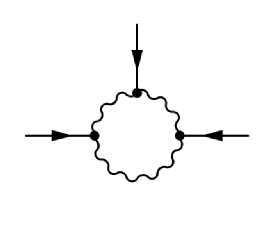
Figure 3: The third-order moment.

Carrying out the frequency convolution in Eq. 49, we extract the leading order contribution from this integral in the large scale and long time limits, namely the limits $k\rightarrow 0$, $k^{\prime}\rightarrow 0$, $\omega\rightarrow 0$, $\omega^{\prime}\rightarrow 0$ for the external momenta and frequencies. Working out the momentum integration in the high-momentum shell $\Lambda_{0}e^{-r}\leq q\leq\Lambda_{0}$, we obtain

$$L^{<}_{3}(r)=\frac{3}{2}K_{d}\frac{\lambda^{3}_{0}D^{3}_{0}}{\nu^{5}_{0}\Lambda^{4-d}_{0}}\frac{e^{(4-d)r}-1}{4-d}.$$ (50)

As before, we consider the iterative nature of the shell elimination scheme in thin shells in the momentum space, and obtain the flow of $L_{3}(r)$ in the form of a differential equation

$$\frac{dL_{3}}{dr}=\frac{3}{2\pi}\frac{\lambda^{3}_{0}D^{3}(r)}{\nu^{5}(r)}\frac{1}{\Lambda^{3}(r)}$$ (51)

for $d=1$. The functions $\nu(r)$ and $D(r)$ being known from Eqs. 24 and 25, the differential equation is solved to obtain

$$L_{3}(r)=\frac{3}{2}\,\frac{\lambda_{0}D^{2}_{0}}{\nu^{2}_{0}\Lambda_{0}^{2}}\,\,e^{2r}$$ (52)

in the asymptotic limit of large $r$.

The corresponding renormalized function $L_{3}(\hat{k};\hat{k}^{\prime})$, being symmetric with respect to interchange of $\hat{k}$ and $\hat{k}^{\prime}$, its frequency dependent expression can be obtained by replacing $(\Lambda_{0}e^{-r})^{-2}$ with the expression

$$k^{-1}k^{\prime-1}f^{-1}\left(\frac{\omega}{k^{z}}\right)f^{-1}\left(\frac{\omega^{\prime}}{k^{\prime z}}\right).$$ (53)

Employing Eq. 42 in 52, we thus obtain

$$L_{3}(\mathbf{k},\omega;\mathbf{k}^{\prime},\omega^{\prime})=\frac{3}{8\pi^{2}}\frac{\lambda_{0}^{5}D_{0}^{4}}{\nu_{0}^{4}}\,\,k^{2}\,k^{\prime 2}\,|G(\mathbf{k},\omega)|^{2}\,\,|G(\mathbf{k}^{\prime},\omega^{\prime})|^{2}.$$ (54)

Using this expression in Eq. 48, the third moment is obtained as

$$W_{3}=\frac{3}{8\pi^{2}}\frac{\lambda_{0}^{5}D_{0}^{4}}{\nu_{0}^{4}}\int\frac{d^{d+1}\hat{k}}{(2\pi)^{d+1}}\int\frac{d^{d+1}\hat{k}^{\prime}}{(2\pi)^{d+1}}\,k^{2}k^{\prime 2}\,G(\hat{k})\,|G(\hat{k})|^{2}\,G(\hat{k^{\prime}})\,|G(\hat{k^{\prime}})|^{2}\,G(-\hat{k}-\hat{k^{\prime}})$$ (55)

where the propagators are treated as renormalized as expressed in Eq. 28 with the renormalized surface tension $\nu(k)$ given by Eq. 26. Performing the frequency integrations over $\omega$ and $\omega^{\prime}$ yields

$$W_{3}=\frac{3}{2}\left(\frac{D_{0}}{2\pi\nu_{0}}\right)^{3/2}\int_{-\infty}^{+\infty}dk_{x}\!\int_{-\infty}^{+\infty}dk^{\prime}_{x}\,\,F(k_{x},k_{x}^{\prime}),$$ (56)

in one dimension, where

$$F(k_{x},k^{\prime}_{x})=\frac{U(k_{x},k^{\prime}_{x})}{V(k_{x},k^{\prime}_{x})}$$ (57)

with

$$U(k_{x},k^{\prime}_{x})=3\left(|k_{x}|^{3}+|k^{\prime}_{x}|^{3}\right)+4|k_{x}+k^{\prime}_{x}|^{3/2}\left(|k_{x}|^{3/2}+|k^{\prime}_{x}|^{3/2}\right)+14|k_{x}|^{3/2}|k^{\prime}_{x}|^{3/2}+|k_{x}+k^{\prime}_{x}|^{3}$$ (58)

and

$$V(k_{x},k^{\prime}_{x})=16\,|k_{x}|\,|k_{x}^{\prime}|\,\left(|k_{x}|^{3/2}+|k_{x}^{\prime}|^{3/2}+|k_{x}+k_{x}^{\prime}|^{3/2}\right)^{3}.$$ (59)

The integrations in Eq. 56 can be decomposed to obtain

$$W_{3}=\frac{3}{2}\left(\frac{D_{0}}{2\pi\nu_{0}}\right)^{3/2}\left[2\int^{\infty}_{\mu}dk_{x}\int^{\infty}_{\mu}dk^{\prime}_{x}\,F(k_{x},k^{\prime}_{x})+2\int^{\infty}_{\mu}dk_{x}\int^{\infty}_{\mu}dk^{\prime}_{x}\,F(-k_{x},k^{\prime}_{x})\right].$$ (60)

where we have set infrared cut offs at $\mu$ as these integrals have infrared divergences. Thus we write

$$W_{3}=\frac{3}{2}\left(\frac{D_{0}}{2\pi\nu_{0}}\right)^{3/2}\left[2I(\mu)+2J(\mu)\right]$$ (61)

where

$$I(\mu)=\int^{\infty}_{\mu}dk_{x}\int^{\infty}_{\mu}dk^{\prime}_{x}\,F(k_{x},k^{\prime}_{x})$$ (62)

and

$$J(\mu)=\int^{\infty}_{\mu}dk_{x}\int^{\infty}_{\mu}dk^{\prime}_{x}\,F(-k_{x},k^{\prime}_{x}).$$ (63)

The infrared divergences in these integrals suggest the following forms

$$I(\mu)=I_{0}\,\mu^{-3/2}$$ (64)

$$J(\mu)=J_{0}\,\mu^{-3/2}$$ (65)

where $I_{0}$ and $J_{0}$ are dimensionless constants.

Substituting from Eqs. (64) and (65) in Eq. (61), we obtain the third moment as

$$W_{3}=3\left(\frac{D_{0}}{2\pi\nu_{0}}\right)^{3/2}(I_{0}+J_{0})\,\frac{1}{\mu^{3/2}}$$ (66)

According to the definition of skewness, we thus obtain from Eqs. 46 and 66

$$S=\frac{W_{3}}{W_{2}^{3/2}}=\frac{3}{8}\,(I_{0}+J_{0})\,\pi^{3/2}.$$ (67)

We calculate the constants $I_{0}$ and $J_{0}$ from Eqs. 62 and 63, using the expressions given by Eqs. 57, 58 and 59, and obtain

$$I_{0}=\lim_{\mu\rightarrow 0^{+}}[\mu^{3/2}I(\mu)]=0.034946$$ (68)

$$J_{0}=\lim_{\mu\rightarrow 0^{+}}[\mu^{3/2}J(\mu)]=0.120089$$ (69)

by means of numerical integrations. The computation shows convergence to the above numerical values as the parameter $\mu$ is chosen to approach values close to zero.

From Eq. 67, the value of skewness is thus found to be

$$S=\frac{3}{8}\,(0.155035)\,\pi^{3/2}=0.323732.$$ (70)

IV Discussion and Conclusion

We employed Yakhot and Orszag’s scheme of renormalization without rescaling and obtained the renormalized surface tension and the strength of the noise correlation for the surface growth problem governed by the KPZ dynamics on a flat substrate. This scheme of renormalization is slightly different from the usual perturbative renormalization group analysis with rescaling that has been employed for dynamical problems by Ma and Mazenko s.k.Ma_prb_11_4077_75 , Forster et al. forster_pra_16_732_77 , and Medina et al. KPZ89 . This method allowed us the advantage of obtaining the flow equations directly without rescaling by considering the iterative nature of the scale elimination procedure. This yielded the fixed point from the $r$-dependent expression of effective coupling constant $g(r)$ in the limit $r\rightarrow\infty$. Similar to the other calculations, the renormalized surface tension and the strength of the noise correlation are found to be renormalized in the same way so that $D(r)/\nu(r)$ is $r$-independent, a consequence of fluctuation dissipation theorem for the case of $(1+1)$ dimensional KPZ equation forster_pra_16_732_77 ; Deker .

To obtain a numerical value for the skewness, we employed the diagrammatic approach for the second and third order moments $W_{2}$ and $W_{3}$. The Fourier integrals of these moments involve the loop integrals $L_{2}$ and $L_{3}$. The simplicity of Yakhot and Orszag’s renormalization scheme allowed us to find renormalized expressions for these loop integrals in a straightforward manner. Although the renormalized diagrams are infrared divergent, the calculated value of skewness turns out to be finite due to cancellation of the infrared cutoff parameter $\mu$. We obtained a value of skewness $S=0.323732$ for the flat geometry in the stationary state which is compared with the results of numerical simulations for various growth models and those of experiments in Table 1. We present a discussion with regard to these results in the following paragraphs.

It has been shown by numerical simulations for polynuclear growth (PNG) that the roughness and growth exponents are in good agreement with the one dimensional KPZ exponents saarloos_86 ; goldenfeld . Further numerical work by Krug et al. J-krug_92 and Bartelt and Evance bartelt_jpa_26_2743_93 have ensured that the PNG model belongs to the universality class of the KPZ growth model Meakin93 . Prähofer and Spohn Michael_Herbert_00 have shown that the PNG model follows the TW distribution with different initial conditions. They estimated the skewness for three different shapes, namely, $S=0.2241$ for the curved shape (GUE TW), $S=0.2935$ for the flat shape (GOE TW), and $S=0.35941$ for the stationary self-similar case Michael_Herbert_00 . On the other hand, the distribution of height fluctuations for the KPZ growth model with sharp wedge initial condition was shown to be the same as that of the GUE TW distribution, as established by Sasamoto and Spohn sasamoto_prl_104_230602_10 ; 2010JSMTE_11_013S . Calabrese and Doussal calabrese_prl_106_250603_11 obtained the GOE TW distribution by mapping the one dimensional KPZ problem with flat initial condition to a one end free directed polymer, referred to as a point-to-line configuration. The curved initial condition, on the other hand, maps on to a point-to-point configuration of the directed polymer.

For the case of directed polymers at zero temperature in a random potential (DPRP), Kim et al. JMKIM introduced two types of random site potentials $\mu(\mathbf{x},t)$, namely, uniform and Gaussian distributions for $\mu(\mathbf{x},t)$, with the bending energy ($\gamma$) of the polymer as the only tunable parameter. They obtained skewness $S=-0.29\pm 0.02$ of the minimum energy distribution in $1+1$ dimensions for uniform distribution of $\mu(\mathbf{x},t)$ for a point-to-line configuration via simulations for $\gamma>1$. The same value of skewness was obtained for Gaussian distribution of $\mu(\mathbf{x},t)$, which is independent of $\gamma$. Kim and others jmkim_prl_62_2289_89 ; JMKIM studied height fluctuations of surface growth using the RSOS model with a flat initial condition where the scaling form of the height distribution matches with the energy distribution of the DPRP within numerical accuracy. The skewness in the same model turned out to be $S\approx-0.29$, suggesting universality of the probability distribution function.

Using a mean field theory in terms of densities at different heights applied to the KPZ equation in $(1+1)$ dimensions, Ginelli and Hinrichsen meanfield started with the flat initial condition $h(x,0)=0$ and obtained the skewness $S=\pm 0.46$ for the transient regime. Takeuchi et al. kazumasa carried out an experiment on a growing interface in liquid crystal turbulence and established that it is in the KPZ universality class. For flat initial conditions, their experimental asymptotic value for skewness was close to $\simeq 0.29$ as suggested by their experimental plots. These values are displayed in Table 1 for comparison with our result.

Table 1: Values of Skewness in one dimension

System of Study	Reference	Methodology	Skewness
SSM (flat)	J-krug_92	Numerical	$0.28\pm 0.04$
SSM (stationary)	J-krug_92	Numerical	$\approx 0.33$
DPRM (point-to-line)	J-krug_92	Numerical	$-0.296\pm 0.028$
DPRP (point-to-line)	JMKIM	Numerical	$-0.29\pm 0.02$
RSOS (flat)	jmkim_prl_62_2289_89 ; JMKIM	Numerical	$\approx-0.29$
TLC (flat)	kazumasa	Experimental	$0.29$
PNG (curved)	Michael_Herbert_00	Numerical	0.2241
PNG (flat)	Michael_Herbert_00	Numerical	$0.2935$
PNG (stationary)	Michael_Herbert_00	Numerical	$0.35941$
KPZ (mean field, flat)	meanfield	Analytical	$\pm 0.46$
Combustion front (flat)	miettinena_epjb_46_55_05	Experimental	$0.33$
Combustion front (stationary)	miettinena_epjb_46_55_05	Experimental	$0.32$
KPZ (present calculation)	Eq. (70)	Analytical	$0.3237$

We observe that our calculated result for the skewness is comparable with some of the experimental values and numerical simulations. It deviates from the non-stationary results and the deviation is more pronounced from the result for curved interfaces. This is expected as our calculations are applicable for a flat geometry in the stationary state. We also observe that the result of the mean field calculation deviates somewhat strongly from all other results. Since skewness is determined by the underlying probability distribution, its calculation following from the governing dynamics is of importance in inferring the universality class. Moreover, the existing studies indicate that the pdf is determined by not only the governing dynamics but also by the boundary conditions. Thus it may be said that there are different subclasses belonging to the same universality class. Different numerical values of skewness may thus be said to correspond to different universality subclasses although they may have the same scaling exponents for the correlation and response functions.

Since the renormalization scheme involves calculations of the statistical moments in the large scale limit $k\rightarrow 0$, such calculations are expected to lead to the statistical properties of the growth process at large scales. The fact that $W_{2}$ and $W_{3}$ turn out to be infrared divergent implies a dominant role of the large scale fluctuations in determining these statistical moments. Moreover since the renormalization scheme involves calculations in the long time limit $\omega\rightarrow 0$, such calculations are expected to capture the statistical properties of the growth process in the stationary state.

However, for a large system, achieving a stationary state is difficult Imamura_prl_108_2012 , especially in experiments and numerical simulations, unless a stationary state is taken as an initial condition Takeuchi_prl_110_2013 . To achieve a stationary pdf for the flat one dimensional KPZ problem, Imamura and Sasamoto took both sided Brownian motion as an initial condition Imamura_prl_108_2012 ; Imamura_JSP_2013 and obtained the generating function for the replica partition function as a Fredholm determinant. This allowed for the calculation of the pdf which was found to approach the Baik-Rains $F_{0}$ distribution in the long time limit. Krug et al. J-krug_92 investigated the stationary state skewness for the SSM model with random uncorrelated spins ($\sigma_{i}=\pm 1$). They obtained $|S|\approx 0.33$ which agrees well with our calculated value. Maunuksela et al. Maunuksela_PRL_79_1515 identified that the universality class of slow combustion fronts of a paper sheet belongs to the KPZ universality class on the basis of scaling exponents. With the same experimental conditions, Miettinena et al. miettinena_epjb_46_55_05 performed an experiment on paper burning to find the skewness from the pdf. They studied the height distribution of combustion fronts for flat initial conditions in the saturation regime and obtained the value $S=0.32$ which agrees well with our calculated value. It may however be noted that Takeuchi coment_Takeuchi_12 has suggested that their analysis of the pdf may need modifications.

Although our calculated value for the skewness ($0.3237$) compares excellently well (within 1–2%) with the above mentioned stationary values ($0.33$ and $0.32$), we observe that there is a slight departure (of about $10\%$) from the value $S=0.3594$ coming from the PNG model Michael_Herbert_00 . This departure may be due to the dominating role of large scale fluctuations in determining the moments $W_{2}$ and $W_{3}$. The infrared cutoff $\mu$ may be interpreted as the inverse of the size $L$ of the substrate and thus the calculations appear to be influenced by finite size effects. In spite of this slight departure, together with the agreements with the experimental results, our calculation for the skewness seems to identify the relevant universality subclass of the KPZ equation.

Ideally speaking, full information about the pdf enables one to classify many seemingly similar problems into varying universality classes. However, an analytical calculation of the full pdf is an extremely difficult task, whereas the calculation of higher order moments such as the skewness is a more viable approach. Thus a classification scheme for universality beyond the scaling exponents can be formulated via the values of skewness for various processes. Takeuchi and Sano K_A_Takeuchi have proved through the TLC experiment that the KPZ class has geometry dependent subclasses in spite of having the same scaling exponents. Thus, to characterize the subclasses, knowledge of skewness and higher order moments is very much essential. The calculation of skewness, directly from the KPZ dynamics, is therefore an important step in identifying a universality subclass of the KPZ equation.

References

- (1) A.-L. Barabási and H. E. Stanley, Fractal Concepts in Surface Growth, (Cambridge University Press, Cambridge, England, 1995).
- (2) J. Krug, Adv. Phys. 46, 139 (1997).
- (3) T. Halpin-Healy and Y.-C. Zhang, Phys. Rep. 254, 215 (1995).
- (4) P. Meakin, Phys. Rep. 235, 189 (1993).
- (5) F. Family and T. Vicsek, J. Phys. A 18, L75 (1985).
- (6) M. Kardar, G. Parisi, and Y.-C. Zhang, Phys. Rev. Lett. 56, 889 (1986).
- (7) Z.-W. Lai and S. Das Sarma, Phys. Rev. Lett. 66, 2348 (1991).
- (8) P. Meakin, P. Ramanlal, L. M. Sander, and R. C. Ball, Phys. Rev. A 34, 5091 (1986).
- (9) M. Plischke and Z. Rácz, Phys. Rev. Lett. 53, 415 (1984).
- (10) R. Jullien and R. Botet, Phys. Rev. Lett. 54, 2055 (1985).
- (11) M. Plischke and Z. Rácz, Phys. Rev. A 32, 3825 (1985).
- (12) M. Plischke, Z. Rácz, and D. Liu, Phys. Rev. B 35, 3485 (1987).
- (13) T. Vicsek, M. Cserző, and V. K. Horváth, Physica A 167, 315 (1990).
- (14) F. Family and T. Vicsek (eds.), Dynamics of Fractal Surfaces, (World Scientific, Singapore, New Jersey, 1991).
- (15) K. A. Takeuchi and M. Sano, Phys. Rev. Lett. 104, 230601 (2010).
- (16) K. A. Takeuchi, M. Sano, T. Sasamoto, and H. Spohn, Sci. Rep. 1, 34 (2011).
- (17) W. van Saarloos and G. H. Gilmer, Phys. Rev. B 33, 4927 (1986).
- (18) N. Goldenfeld, J. Phys. A 17, 2807 (1984).
- (19) J. Krug and H. Spohn, Phys. Rev. A 38, 4271 (1988).
- (20) M. Prähofer and H. Spohn, Phys. Rev. Lett. 84, 4882 (2000).
- (21) D. Forster, D. R. Nelson, and M. J. Stephen, Phys. Rev. A 16, 732 (1977).
- (22) Y. Kuramoto, Chemical Oscillations, Waves, and Turbulence, (Dover Publications, 2003).
- (23) G. I. Sivashinsky, Acta. Astron. 4, 1177 (1977).
- (24) D. S. Fisher and D. A. Huse, Phys. Rev. B 43, 10728 (1991).
- (25) M. Kardar and Y.-C. Zhang, Phys. Rev. Lett. 58, 2087 (1987).
- (26) J. M. Kim, M. A. Moore, and A. J. Bray, Phys. Rev. A 44, 2345 (1991).
- (27) D. A. Huse, C. L. Henley, and D. S. Fisher, Phys. Rev. Lett. 55, 2924 (1985).
- (28) D. A. Huse and C. L. Henley, Phys. Rev. Lett. 54, 2708 (1985).
- (29) A. R. Kerstein and W. T. Ashurst, Phys. Rev. Lett. 68, 934 (1992).
- (30) E. Medina, T. Hwa, M. Kardar, and Y.-C. Zhang, Phys. Rev. A 39, 3053 (1989).
- (31) R. Baiod, D. Kessler, P. Ramanlal, L. Sander, and R. Savit, Phys. Rev. A 38, 3672 (1988).
- (32) P. Pfeifer, D. Avnir, and D. Farin, Surf. Sci. 126, 569 (1983).
- (33) M. Moskovits, Rev. Mod. Phys. 57, 783 (1985).
- (34) F. Colaiori and M. A. Moore, Phys. Rev. Lett. 86, 3946 (2001).
- (35) H. van Beijeren, R. Kutner, and H. Spohn, Phys. Rev. Lett. 54, 2026 (1985).
- (36) T. Hwa and E. Frey, Phys. Rev. A 44, R7873 (1991).
- (37) M. Lässig, Phys. Rev. Lett. 80, 2366 (1998).
- (38) M. Schwartz and S. F. Edwards, Europhys. Lett. 20, 301 (1992).
- (39) L. Canet, H. Chaté, B. Delamotte, and N. Wschebor, Phys. Rev. Lett. 104, 150601 (2010).
- (40) T. Kloss, L. Canet, and N. Wschebor, Phys. Rev. E 86, 051124 (2012).
- (41) M. A. C. Huergo, M. A. Pasquale, P. H. González, A. E. Bolzán, and A. J. Arvia, Phys. Rev. E 84, 021917 (2011).
- (42) M. A. C. Huergo, M. A. Pasquale, A. E. Bolzán, A. J. Arvia, and P. H. González, Phys. Rev. E 82, 031903 (2010).
- (43) F. D. A. Aarão Reis, Phys. Rev. E 70, 031607 (2004).
- (44) J. Krug, P. Meakin, and T. Halpin-Healy, Phys. Rev. A 45, 638 (1992).
- (45) T. Sasamoto and H. Spohn, Phys. Rev. Lett. 104, 230602 (2010).
- (46) T. Sasamoto and H. Spohn, J. Stat. Mech. P11013 (2010).
- (47) F. Ginelli and H. Hinrichsen, J. Phys. A: Math. Gen. 37, 11085 (2004).
- (48) V. Yakhot and S. Orszag, J. Sci. Comput. 1, 3 (1986).
- (49) P. C. Hohenberg and B. I. Halperin, Rev. Mod. Phys. 49, 435 (1977).
- (50) V. Yakhot and S. A. Orszag, Phys. Rev. Lett. 57, 1722 (1986).
- (51) E. Frey and U. C. Täuber, Phys. Rev. E 50, 1024 (1994).
- (52) S.-K. Ma and G. F. Mazenko, Phys. Rev. B 11, 4077 (1975).
- (53) U. Deker and F. Haake, Phys. Rev. A 11, 2043 (1975).
- (54) M. C. Bartelt and J. W. Evans, J. Phys. A. 26, 2743 (1993).
- (55) P. Calabrese and P. Le Doussal, Phys. Rev. Lett. 106, 250603 (2011).
- (56) J. M. Kim and J. M. Kosterlitz, Phys. Rev. Lett. 62, 2289 (1989).
- (57) T. Imamura and T. Sasamoto, Phys. Rev. Lett. 108, 190603 (2012).
- (58) K. A. Takeuchi, Phys. Rev. Lett. 110, 210604 (2013).
- (59) T. Imamura and T. Sasamoto, J. Stat. Phys. 150, 908 (2013).
- (60) J. Maunuksela, M. Myllys, O.-P. Kähkönen, J. Timonen, N. Provatas, M. J. Alava, and T. Ala-Nissila, Phys. Rev. Lett. 79, 1515 (1997).
- (61) L. Miettinena, M. Myllys, J. Merikoski, and J. Timonen, Eur. Phys. J. B 46, 55 (2005).
- (62) K. A.Takeuchi, preprint (2012).