How nanochannel confinement affects the DNA melting transition within the Poland-Scheraga model

Abstract

When double-stranded DNA molecules are heated, or exposed to denaturing agents, the two strands get separated. The statistical physics of this process has a long history, and is commonly described in term of the Poland-Scheraga (PS) model. Crucial to this model is the configurational entropy for a melted region (compared to the entropy of an intact region of the same size), quantified by the loop factor. In this study we investigate how confinement affects the DNA melting transition, by using the loop factor for an ideal Gaussian chain. By subsequent numerical solutions of the PS model, we demonstrate that the melting temperature depends on the persistence lengths of single-stranded and double-stranded DNA. For realistic values of the persistence lengths the melting temperature is predicted to decrease with decreasing channel diameter. We also demonstrate that confinement broadens the melting transition. These general findings hold for the three scenarios investigated: namely 1. homo-DNA, i.e. identical basepairs along the DNA molecule; 2. random sequence DNA, and 3. “real” DNA, here T4 phage DNA. We show that cases 2 and 3 in general give rise to broader transitions than case 1. Case 3 exhibits a similar phase transition as case 2 provided the random sequence DNA has the same ratio of AT to GC basepairs. A simple analytical estimate for the shift in melting temperature is provided as a function of nanochannel diameter. For homo-DNA, we also present an analytical prediction of the melting probability as a function of temperature.

I Introduction

The three dimensional structure of double-stranded Deoxyribonucleic acid (dsDNA) DNA is the famed Watson-Crick double-helix, within a broad range of salt and temperature conditions.watsoncrick This double-helix encodes the genetic information of an entire organism in terms of four types of bases. Base complementarity guarantees that the same information is contained in the two strands of a dsDNA.alberts

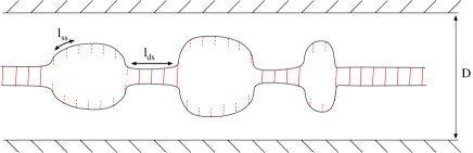
Figure 1: Cartoon of DNA melting in a nanochannel. A given microstate of DNA, at elevated temperatures, is an alternating set of intact double-stranded regions and melted single-strand regions (DNA bubbles). Within the Poland-Scheraga model, the statistical physics of DNA melting is described in terms of two hydrogen-bond energies, ten stacking (nearest neighbor) parameters and the loop factor $g(m)$ which quantifies the conformational entropy for a melted region corresponding to $m$ basepairs (relative to the entropy of an unmelted region of the same size). The functional form of $g(m)$ is different for unconfined and nanoconfined DNA.

By temperature increase the double-stranded double-helical DNA progressively denatures – DNA melting, see Figure 1. Partially melted DNA is an alternating set of intact, stiff, double-stranded regions (persistence length about 50 nm) and of single-stranded, floppy (persistence length about 1 to a few nm), “melted” regions (DNA bubbles).poland Each of these regions is subject to thermal fluctuations. Interestingly, the average free energy associated with breaking an AT-basepair is smaller than the corresponding energy for a GC-basepair.gueron In melting studies, therefore, DNA tends to melt first in AT-rich regions ($45.79$ ^∘C at salt concentration 0.01 M for pure AT) and only at higher temperature ($95.88$ ^∘C at salt concentration 0.01 M for pure GC regions) in GC-rich regions.

On the theoretical side, The Poland-Scheraga (PS) model of DNA melting has been proven to well reproduce (macroscopic) melting data.poland ; yeramian ; santalucia ; FKreview ; wartell ; blake ; blossey Note, however, that there is an alternative model, the Peyrard-Bishop model,peyrard ; Kalosakas_Rasmussen see Ref. FKreview, for a comparative study of the two models. Herein we use the PS model, which is an Ising model with a long-range term due to the entropy associated with the melted single-stranded regions, and has the following parameters: two hydrogen bond (Watson-Crick) energies (AT or GC bonds), ten independent stacking (nearest neighbor) parameters, the loop factor (or, loop functionblake ), and the ring-factor (bubble initiation) parameter (related to the cooperativity parameter).poland Rather recently the ten stacking parameters were independently measured for the first time for different temperatures and salt concentrations.FK

Theoretical interest in the melting transition originates, in part, from the fact that the PS model exhibits a phase-transition which can be analyzed exactly.fisher_84 ; Wiegel This analysis treats unconfined DNA molecules, with identical hydrogen bond and stacking energies (homo-DNA). For unconfined DNA the loop factor $g(m)$ (see above) scales with DNA bubble size $m$ as a power-law: $g(m)\simeq m^{-c}$ with a loop exponent $c$. The exponent $c$ determines the order of the phase transition; if $c>2$ the melting transition is first order.kafri

More recent studieshwa ; garel_04 ; giacomin2009 ; alexander2009 ; derrida2014 address the challenge of understanding how the DNA sequence affects the melting transition, typically by analyzing the melting of random sequence DNA.derrida_83 ; azbelI ; azbelII ; azbelIII ; lifshitz Unlike for the case of homo-DNA melting, no exact results exist for these kinds of systems.

Herein, we go beyond previous studies by considering how confinement affects the DNA melting transition. In particular, we seek to quantify how confinement affects the DNA melting temperature and the width of the melting transition. In contrast to Ref. li_2014, , where molecular dynamics simulations of very short DNA (15 basepairs) were performed, we are here interested in the thermodynamic limit (we study typical DNA sizes of $2\cdot 10^{5}$ basepairs). In Ref. werner_schad2015, we calculate how confinement influences $g(m)$ and show how this influences melting for a highly simplified model system. In the present study, we go beyond Ref. werner_schad2015, by calculating what consequences the effect of confinement on $g(m)$ has for the melting of a more realistic model of DNA. Using as input the functional form for $g(m)$,werner_schad2015 we provide results of extensive simulations within the Poland-Scheraga model for 1. homo-DNA, 2. random sequence DNA and 3. “real” DNA (T4 phage). We also provide a simple formula for estimating how the melting temperature changes as a function of the channel diameter and present an analytical prediction of the melting probability of homo-DNA as a function of temperature.

The present study is inspired by recent experiments which demonstrate the potential to study local properties of the DNA melting transition in nanochannels.reisner2010 ; reisner2012 Other recent experiments now allow studying also the DNA melting dynamics.altan ; our_prl

The biological relevance of DNA melting in confined environments is, for instance, due to the fact that local denaturation of DNA is necessary for protein binding to a DNA single-strand,mark ; mark1 and is implicated in transcription initiation.kalo ; yeramian

II Review of the Poland-Scheraga model

In this section we introduce the Poland-Scheraga (PS) model for unconfined DNA. In the next section we discuss how the PS model must be modified in order to study DNA melting under confinement.

II.1 General considerations

Consider double-stranded DNA with $N$ internal basepairs, that are clamped at both ends for simplicity (Fig. 1). The free energy required for breaking a hydrogen bond at basepair $i$ is denoted by $E_{\rm hb}(i)$. There are two values for this parameter (AT-bonds or GC-bonds). For disrupting the stacking (nearest neighbor) interactions between basepairs $i-1$ and $i$ there is a free energy cost $E_{\rm st}(i-1,i)$. There are ten stacking parameters.FK In addition we need the ring factor $\xi\approx 10^{-3}$ (see Ref. FK, ) which is a Boltzmann factor associated with the free energy cost of creating two “boundaries” between intact and melted DNA. Note that $E_{\rm hb}(i)$ and $E_{\rm st}(i-1,i)$ have energetic as well as entropic contributions: $E_{\rm hb}(i)=U_{\rm hb}(i)-TS_{\rm hb}$ and $E_{\rm st}(i-1,i)=U_{\rm st}(i-1,i)-TS_{\rm st}$, where $U$ denote energetic contributions, $T$ is the temperature and $S_{\rm hb}$ and $S_{\rm st}$ are entropies, commonly assumed to be basepair independent. Finally, the Poland-Scheraga model requires as input the ratio of the number of configurations for a melted region (DNA bubble) and the number of configurations of an intact region, quantified by the loop factor $g(m)$, see sections III.1 and III.2.

II.2 The melting temperature and the Marmur-Doty formula

Throughout the main text we repeatedly refer to the melting temperature, $T_{M}$, or deviations therefrom. $T_{M}$ is defined as the temperature where the melting probability = 1/2.

We can estimate the melting temperature, $T_{M}$ by setting the total free energy per basepair, $E_{\rm hb}+E_{\rm st}$, equal to zero. This leads to

$$T_{\rm M}=(U_{\rm hb}+U_{\rm st})/S_{\rm ref}$$ (1)

with $S_{\rm ref}=S_{\rm hb}+S_{\rm st}$, and we find that the free energy can also be expressed as

$$E=S_{\rm ref}(T_{\rm M}-T).$$ (2)

The total free energy of a given DNA sequence can be estimated as the sum of the free energies of the AT and the GC portion:

$$E = f_{\rm AT}\Delta E_{\rm AT}+f_{\rm GC}\Delta E_{\rm GC}$$ (3)

$$= S_{\rm ref}(f_{\rm AT}T_{\rm AT}+f_{\rm GC}T_{\rm GC}-T)$$

with the free energy of random AT and random GC sequences $\Delta E_{\rm AT}$ and $\Delta E_{\rm GC}$.

With Eq. (2) we find the Marmur-Doty formula, which gives a simple estimate for the melting temperature, $T_{M}$ of unconfined DNA:

$$T_{\rm MD}=f_{\rm AT}T_{\rm AT}+f_{\rm GC}T_{\rm GC}$$ (4)

where $f_{\rm AT/GC}$ is the fraction of AT/GC bonds in the DNA sequence. $T_{\rm AT/GC}$ is the melting temperature for pure random AT/GC sequences. We note that this formula is rather crude, in reality $T_{\rm M}$ depends weakly also on $\xi$ and $g(m)$.

We will later use the stability parameters introduced in Sec. II.1 from Ref. FK, (Table 1). Herein, the ten stacking parameters were experimentally determined and the hydrogen bond energies were found from the empirical Marmur-Doty melting temperature together with Eq. (2) and

$$E_{\rm hb}^{\rm AT}=\Delta E_{\rm AT}-\frac{1}{4}\sum_{AT,TA,AA,TT}E^{\rm st}$$ (5)

and the corresponding equation for GC. Note that we use a different notation than as Ref. FK, , $E=-\Delta G$ and $S_{\rm ref}=-\Delta S$.

For homo-DNA, the melting temperature is estimated as:

$$T_{\rm M}^{\rm A} = \frac{U_{\rm st}^{\rm AA}+U_{\rm hb}^{\rm AT}}{S_{\rm hb}+S_{\rm st}}$$ (6)

$$= T_{\rm AT}+\frac{1}{4S_{\rm ref}}(U_{\rm st}^{\rm AT}+U_{\rm st}^{\rm TA}-2U_{\rm st}^{\rm AA}).$$ (7)

At salt concentration 0.01 M, we have $T_{\rm M}^{\rm A}=52.73^{\circ}$C.

Even though investigation of unconfined DNA is not the main purpose of this study, we elaborate a bit on deviations from the Marmur-Doty formula in appendix C, where we also investigate the properties of the DNA melting temperature on the value of $c$ for unconfined DNA.

III The loop factor

In this section we give details about the loop factor for confined and unconfined DNA molecules.

III.1 Loop factor for unconfined DNA

Let us now consider $g(m)$ for unconfined DNA (see also Ref. werner_schad2015, ). For simplicity, assume that the melted DNA region is described by a self-avoiding random walk of $2m$ steps in 3 dimensions on a lattice. If we denote by $z$ the coordination number (number of nearest neighbors in the absence of self-exclusion), and limit ourselves to large number of steps, the number of configurations for a closed loop (ring polymer) is $\Omega_{\rm ring}=z^{2m}m^{-c}$, where $c=1.76$. For a linear polymer (intact DNA), similarly $\Omega_{\rm linear}=\tilde{z}^{m}$, with a different coordination number $\tilde{z}$, since the persistence length is in general different for double-stranded DNA compared to single-stranded DNA. The prefactor $(z/\tilde{z})^{2m}$ is included in formalism by a redefinition of the the Watson-Crick energy $E_{\rm hb}\rightarrow E_{\rm hb}+2RT\log(z/\tilde{z}^{1/2})$ and the loop factor then becomes

$$g_{u}(m)\sim m^{-c}$$ (8)

for unconfined DNA. If one includes self-avoidance between intact DNA regions and melted regions one finds $c=2.12$kafri . For an unconfined ideal (phantom) chain one obtains $c=3/2$. A few words of caution are here needed. Strictly speaking, the quantity $g(m)$ is proportional to the number of configurations of a random walk of $2m$ steps with the same start and end point, where the random walk is constrained to have no bound complementary basepairs along its path.werner_schad2015 We here follow the approximation common to the literature,kafri namely, assuming that $g(m)$ can be estimated by removing the constraint of no bound states. In Ref. werner_schad2015, we discuss the effects caused by including the constraint mentioned above.

The power-law form for $g_{u}(m)$ gives rise to an effectively long-range interaction for molten DNA regions.blake ; fixman ; richard Note that the persistence length of single-stranded DNA is 1-5 nm. So, the loop-correction $g(m)\sim m^{-c}$ should not be included for small bubbles, although it is common practice to include it for all $m$-values. A weight of $\xi g(m)$ is assigned to each bubble. Therefore the value of the ring factor $\xi$ from Ref. FK, , which was obtained from very small DNA molecules neglecting the loop-correction, has to be complemented by a loop factor $g_{u}(m)=m^{-c}$. We note that a useful form for $g(m)$ approximately correct for all $m$ is given in, for instance, Ref. wartell, .

III.2 Loop factor for DNA confined in a nanochannel

The aim of this study is to understand how channel confinement influences the melting transition for real DNA. To that end we need to find a functional form for $g(m)$ for a polymer confined to a nanochannel. In general we have:

$$g_{c}(m)=\frac{G_{\rm ss}(N_{\rm ss})}{G_{\rm ds}(N_{\rm ds})}$$ (9)

The quantity $G_{\rm ds}(N_{\rm ds})$ is Green’s function for a double-stranded DNA consisting of $N_{\rm ds}$ Kuhn lengths in a square channel with side length $D$ and random initial positions for the polymer start position. Similarly, $G_{\rm ss}(N_{\rm ss})$ is proportional to Green’s function for a single-stranded DNA region of $N_{\rm ss}$ Kuhn lengths with identical start and end positions [below we determine the constant of proportionality using known asymptotic results for $g(m)$]. The number of base pairs is denoted by $m$ and related to the Kuhn lengths according to $N_{\rm ss}=2m/(x\ell_{\rm ss})$ and $N_{\rm ds}=m/(x\ell_{\rm ds})$ with a conversion factor $x=3{\rm bp/nm}$ (the center-to-center distance between adjacent basepairs is $0.34$ nm, see Ref. alberts, ). We use $\ell_{\rm ss}=6{\rm nm}$ for single-stranded DNA and $\ell_{\rm ds}=100{\rm nm}$ for double-stranded DNA throughout this study. Determining $G_{\rm ds}(N_{\rm ds})$ and $G_{\rm ss}(N_{\rm ss})$ poses the formidable, unsolved, task of deriving an expression for the number of conformations for a worm-like chain modelkhokhlov with two constraints: (i) no polymer conformations can “pass” the channel walls, and (ii) the polymer conformations cannot self-intersect. In order to provide expressions for $G_{\rm ss}(N_{\rm ss})$ we neglect self-avoidance, i.e., the constraint (ii) above. Notice that for typical experimental channel sizes, $D\sim 50-100$ nm,reisner_pedersen_2012 thus $\ell_{\rm ss}/D\ll 1$. Single-stranded regions are therefore well described by the statistics of an ideal Gaussian chain, and $G_{\rm ss}(N_{\rm ss})$ is given by the solution to a diffusion equation.khokhlov ; werner2013 The result is given in the Supplementary Information of Ref. werner_schad2015, , where we find that for an ideal Gaussian chain we have

$$G_{\rm ss}(N_{\rm ss}) =AN_{\rm ss}^{-1/2}\left[\sum_{k=1}^{\infty}\exp\left(-\Lambda^{\rm ss}_{k}N_{\rm ss}\right)\right]^{2},$$ (10)

$$\Lambda^{\rm ss}_{k} =\frac{\ell_{\rm ss}^{2}\pi^{2}k^{2}}{6D^{2}}.$$ (11)

where $\Lambda^{\rm ss}_{k}$ are the eigenvalues of the diffusion operator. The constant of proportionality, $A$, is obtained below.

For deriving an expression for $G_{\rm ds}(N_{\rm ds})$ we notice that, in contrast to $\ell_{\rm ss}/D$, the ratio of double-strand Kuhn length to channel diameter, $\ell_{\rm ds}/D$, is not necessarily a small number for realistic channels sizes. To address this issue we write

$$G_{\rm ds}(N_{\rm ds})=\gamma(N_{\rm ds})G^{\rm diff}_{\rm ds}(N_{\rm ds})$$ (12)

where

$$G^{\rm diff}_{\rm ds}(N_{\rm ds}) =\left[\frac{8}{\pi^{2}}\sum_{k=0}^{\infty}\frac{1}{(2k+1)^{2}}\exp\left(-\Lambda^{\rm ds}_{2k+1}N_{\rm ds}\right)\right]^{2},$$ (13)

$$\Lambda^{\rm ds}_{k} =\frac{\ell_{\rm ds}^{2}\pi^{2}k^{2}}{6D^{2}}.$$ (14)

The quantity $G^{\rm diff}_{\rm ds}(N_{\rm ds})$ is the Green’s function for an ideal Gaussian chain in weak confinement ($D\gg\ell_{\rm ds}$).werner_schad2015 The factor $\gamma(N_{\rm ds})$ quantifies deviations between the true statistics for a double-stranded region and the ideal Gaussian case. In order to estimate $\gamma(N_{\rm ds})$ we note that in Ref. tree_2013, an interpolation formula for the free energy of confinement was given which encompasses both the Odijk regime and the diffusive regime of an ideal worm-like chain. We here choose $\gamma(N_{\rm ds})$ so that the free energy of confinement, $R\log[G_{\rm ds}(N_{\rm ds})]$, equals the one given in Eq. (13) of Ref. tree_2013, , in the limit $N_{\rm ds}\to\infty$. We then have

$$\gamma(N_{\rm ds}) =\exp\left(2\Lambda^{\rm ds}_{1}\left(1-\kappa(\ell_{\rm ds}/D)\right)N_{\rm ds}\right),$$ (15)

$$\kappa(z) =\left(1+1.672z+1.287z^{2}\right)^{-2/3}.$$ (16)

In the derivation of the above expressions, we have assumed that the entropy of an intact or melted section in the interior of a polymer is the same as that of an isolated polymer of the same size. We briefly discuss the effect of this assumption in the Supplemental Material of Ref. werner_schad2015, .

Our final task is now to determine the constant $A$ in Eq. (10). To that end we require that $g_{c}(m)$ agrees with the unconfined case for a ideal chain, $g_{u}(m)=m^{-3/2}$, as $D\rightarrow\infty$. In order to analyze the large $D$ limit of $g_{c}(m)$, Eqs. (10) and (13) are not suitable. We therefore rather use the equivalent resummed expressions

$$G_{\rm ss}(N_{\rm ss})=AN_{\rm ss}^{-1/2}\left[\sqrt{\frac{6D^{2}}{\ell_{\rm ss}^{2}\pi N_{\rm ss}}}\left(\sum_{n=1}^{\infty}\exp\left(-\frac{6D^{2}n^{2}}{\ell_{\rm ss}^{2}N_{\rm ss}}\right)+\frac{1}{2}\right)-\frac{1}{2}\right]^{2}$$ (17)

$$G^{\rm diff}_{\rm ds}(N_{\rm ds})=\left[1-\frac{2}{\sqrt{B}}\left(\frac{1}{\sqrt{\pi}}+2\sum_{n=1}^{\infty}(-1)^{n}\left\{\sqrt{\pi}\exp\left(-Bn^{2}\right)-\sqrt{B}n\operatorname{erfc}\left(\sqrt{B}n\right)\right\}\right)\right]^{2}\quad\textrm{with}\quad B=\frac{3D^{2}}{2\ell_{\rm ds}^{2}N_{\rm ds}}$$ (18)

where Eq. (17) was obtained using the Poisson resummation formula, and Eq. (18) is derived in Ref. carslaw, (chap. 3). With $\lim_{D\rightarrow\infty}G_{\rm ds}(N_{\rm ds})=1$ we find

$$A=\frac{2\pi}{3}\left(\frac{2}{x\ell_{\rm ss}}\right)^{3/2}\left(\frac{\ell_{\rm ss}}{D}\right)^{2}$$ (19)

With this result, the known value of the ring factor for free DNA $\xi=10^{-3}$ can be used.

The above expressions for $g(m)$ for a channel allow us to obtain numerical results for the melting behavior. To that end we use the Fixman-Freire approximation with stability parameters from Ref. FK, , see appendix A.2 for details. In practice only the first term of the sums in Eqs. (9) - (18) ($k=1$ and $n=1$) are sufficient (we denote them by $G_{\rm ss}^{(2)}$, $G_{\rm ds}^{(2)}$, $G_{\rm ss}^{(1)}$ and $G_{\rm ds}^{(1)}$ in the following). We use $g_{c}(m)=G_{\rm ss}^{(1)}/G_{\rm ds}^{(1)}$ for small bubbles with size $m<m_{0}$, $g_{c}(m)=G_{\rm ss}^{(1)}/G_{\rm ds}^{(2)}$ for the intermediate range with bubbles of size $m_{0}<m<m_{1}$ and $g_{c}(m)=G_{\rm ss}^{(2)}/G_{\rm ds}^{(2)}$ for large bubbles with size $m>m_{1}$. The transition points $m_{0}$ and $m_{1}$ are found numerically as $m_{0}=0.7(D/\ell_{\rm ss})^{2}$ and $m_{1}=17.2(D/\ell_{\rm ss})^{2}$ with maximum errors $0.016\%$ and $0.004\%$. Also, we “pull out” the first term in Eq. (10) and in Eq. (13) and redefine the hydrogen bond energies accordingly (see subsection III.1), i.e., we write

$$g_{c}(m)=f(m)\exp\left(\Big{(}\frac{2\Lambda^{\rm ds}_{1}}{x\ell_{\rm ds}}\kappa(\ell_{\rm ds}/D)-\frac{4\Lambda^{\rm ss}_{1}}{x\ell_{\rm ss}}\Big{)}m\right)$$ (20)

Using the explicit form of the eigenvalues of the diffusion operator, we have

$$g_{c}(m)=f(m)\exp\left(\frac{\pi^{2}}{3xD^{2}}\left(\ell_{\rm ds}\kappa(\ell_{\rm ds}/D)-2\ell_{\rm ss}\right)m\right)$$ (21)

where we introduced a shifted loop factor $f(m)$. Introducing $f(m)$ and the associated redefinition of the hydrogen bond energies (compare to subsection III.1), allows us to avoid numerical problems with the FF algorithm due to multiplication of exponentially small numbers. The function $f(m)$ is plotted in Fig. 2, where we see that for small bubbles we have $f(m)\propto m^{-3/2}$, whereas for large $m$ we have $f(m)\propto m^{-1/2}$. The full functional form smoothly interpolates between these two extremes. In Ref. werner_schad2015, we show that $f(m)$ has a simple interpretation as being proportional to the probability that a confined polymer forms a loop.

In the derivation of the loop factor $g(m)$ we make a number of simplifying assumptions. In particular, the ideal chain approximation is not a very realistic description of single stranded DNA. However, in Ref. werner_schad2015, we find in simulations of a simple model of DNA that the effect of confinement on the melting transition is qualitatively similar for ideal and self-avoiding chains. For this reason, we expect that the $g(m)$ used herein provides qualitatively correct predictions for the effect of channel confinement on the melting transition of DNA.

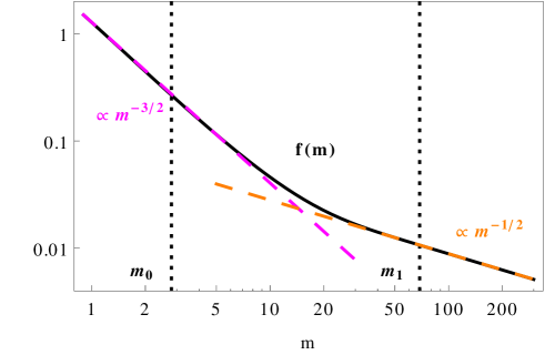
Figure 2: Shifted loop factor $f(m)$ for a polymer confined to a square channel of diameter $D$. The black solid curve shows the exact result for an ideal chain contained in Eqs. (9)–(18). In general we identified three regimes separated by transition points $m_{0}$ and $m_{1}$ (see main text). For small and large $m$ we have that a power-law behavior, $f(m)\propto m^{-3/2}$ and $f(m)\propto m^{-1/2}$, respectively. For illustrative purposes we used a small value for the ratio of channel diameter and single-stranded DNA persistence length, $D/\ell_{\rm ss}=2$.

IV Results

The functional form for the loop factor $g(m)$ presented in the previous section allows us to study how the melting transition changes as the channel diameter is varied. We limit ourself to long DNA molecules (thermodynamic limit) and study melting of three types of prototypical DNA: 1. Homo-DNA, i.e. all basepairs are identical. For this case we obtain analytical estimates alongside the numerical results. 2. Random DNA, i.e., the A, T, G or C basepairs are chosen with probabilities, $p_{A/T}$ and $p_{G/C}=1-p_{A/T}$. 3. Finally, we consider a “real” DNA sequence, namely that of T4 phage DNA. The numerical results are obtained by solving the Poland-Scheraga model (Fixman-Freire approximation) using the functional form for $g(m)$ given above. Details are found in appendix A.

IV.1 homo-DNA

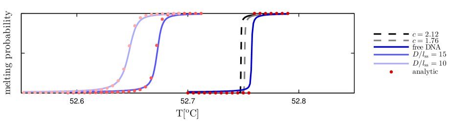
Figure 3: Melting probability as a function of temperature for homo DNA at different channel diameters. Numerical results (solid lines) and the analytical prediction (red marks) from Eq. (25). Notice that decreasing the channel diameter leads to a decrease in the melting temperature and to a broadening of the melting curves. The analytical prediction agrees rather well with the numerical results already for moderate confinement. Dashed lines show melting probabilities for different values of the loop exponent $c$. We see only a very slight change of the width of the transition, for further details on the effect of $c$ and comparison to the analytic prediction see figs. 11 and 12 in the appendix. Parameters: number of basepairs = $2\cdot 10^{5}$, input sequence = ‘AAAAA … AAAA’, and salt concentration = 0.01 $M$. Note that ’free DNA’ here refers to the case $c=1.5$ (unconfined ideal polymer).

We first consider homo-DNA, i.e. assume that the parameters $E_{\rm hb}(i)$ and $E_{\rm st}(i-1,i)$, see subsection II.1, are independent on $i$. We first present analytical estimates for the melting curve, the melting temperature, and the width of the melting curve for small channels, before comparing to numerical results.

In the limit of small channels (or large bubbles), Eq. (9) becomes

$$\lim\limits_{m\to\infty}g_{c}(m) =\frac{G_{\rm ss}^{(2)}}{G_{\rm ds}^{(2)}}=\frac{\pi^{4}}{64}\left(\frac{2m}{x\ell_{\rm ss}}\right)^{-1/2}$$

$$\times\!A\exp\left(\frac{\pi^{2}}{3xD^{2}}\left(\ell_{\rm ds}\kappa(\ell_{\rm ds}/D)-2\ell_{\rm ss}\right)m\right)$$ (22)

Using this approximation, we can derive a number of exact results.

First, there is a channel induced shift in the melting temperature: as discussed in the previous section, the exponential term in Eq. (21) can be included in the hydrogen bond energies, $E_{\rm hb}\rightarrow E_{\rm hb}-RT\frac{\pi^{2}}{3xD^{2}}\left(\ell_{\rm ds}\kappa(\ell_{\rm ds}/D)-2\ell_{\rm ss}\right)$ in analogy with how we included the coordination number in Sec. III.1. This leads to a shift of the melting temperature according to

$$T_{\rm{M,confined}}=\frac{U}{S}=\frac{S_{\rm{ref}}}{S_{\rm{ref}}-\Delta S}T_{\rm M}$$ (23)

with

$$\Delta S=\Delta S_{\rm ss}-\Delta S_{\rm ds}=R\frac{\pi^{2}}{3xD^{2}}\left(\ell_{\rm ds}\kappa(\ell_{\rm ds}/D)-2\ell_{\rm ss}\right)$$ (24)

and where $R$ is the molar gas constant. Confining an ideal (linear) chain to a channel decreases the entropy by an amount $\Delta S_{\rm ss}$ per link for the single-stranded (melted) region and $\Delta S_{\rm ds}$ for the intact double stranded region. This entropy of confinement agrees with a scaling argument given in section I.1.3 in Ref. degennes, . For $\ell_{\rm ds}\kappa(\ell_{\rm ds}/D)>2\ell_{\rm ss}$ we predict that there is an entropy driven decrease in melting temperature for small channels. In particular, we show in Fig. 4 that for typical experimental channel sizes, confinement indeed decreases the melting temperature of DNA. Moreover, we find that the melting temperature as a function of $\ell_{\rm ss}/D$ has a minimum at around $\ell_{\rm ss}/D\approx 0.12$. Within our model, this finding follows from the fact that a double-stranded region enters the Odijk regime (where the entropy of confinement scales as $(\ell_{\rm ds}/D)^{2/3}$ per Kuhn length [see Eqs. (13-16)], rather than as $(\ell_{\rm ds}/D)^{2}$ as for the Gaussian chain regime) at a larger value of $D$ than a single-stranded region. Note that we for the single-stranded region actually do not include the Odijk regime in our expression for the associated Green’s function. Hence, we cannot realistically consider larger values for $\ell_{\rm ss}/D$ than those shown in Fig. 4. We here note that in the simplified model in Ref. werner_schad2015, the persistence length of single-stranded and double-stranded regions are the same which rather leads to a slight increase of the melting temperature for decreasing channel diameters.

Second, once we have redefined the melting temperature, we can in fact predict the full melting curve. To that end we define an effective ring factor as $\xi_{\rm eff}=(\pi^{4}/64)(x\ell_{\rm ss}/2)^{1/2}A\xi=K(\ell_{\rm ss}/D)^{2}\xi$, with $K=\pi^{5}/(48x\ell_{\rm ss})$; for $\ell_{\rm ss}$= 6 nm we have $K=0.354$. Then the problem at hand becomes that of melting with a loop factor $\sim m^{-1/2}$ (“one dimensional” random walk) and ring factor $\xi_{\rm eff}$ (all valid for small channels). The change in the value of the ring-factor, $\xi\rightarrow\xi_{\rm eff}$, is again due to entropic confinement effects. We here restrict ourselves to $D$ values such that $D/\ell_{\rm ss}\geq 7$, for which we have $\xi_{\rm eff}<\xi$. For smaller values of values of $D/\ell_{\rm ss}$ the diffusion approximation used for the single-stranded regions breaks down, see previous section. Using standard analytical techniques (appendix B) we find that the expected fraction of melted basepairs is given by:

$$P=1-\frac{1}{1+\sigma_{0}\beta^{-1}z_{0}{\rm Li}_{c-1}(z_{0})}$$ (25)

where $c=c_{\rm 1d}=1/2$ and $\beta=\exp[\Delta S(T-T_{\rm M,confined})/(RT)]$ with the “universal” dimensionless DNA constant $\Delta S/k_{B}\approx 12.51$ [since $R=1.987$ cal/(mol K) and the entropy loss is $\Delta S=24.85$ cal/(mol K), see Ref. FK, ]. The quantity $\sigma_{0}=\xi_{\rm eff}\exp[-E_{\rm st}/(GT)]$ is the cooperativity parameter, here modified to take into account effects due to the channel (through $\xi_{\rm eff}$). The quantity $z_{0}$ is obtained by solving Eq. (47) numerically; whenever no root $z_{0}$ is found in the interval $0<z_{0}<1$, one sets $P=1$.

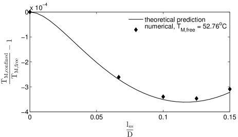
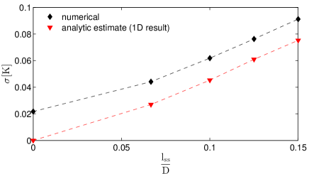
Figure 4: Confinement induced shift in melting temperature (units of Kelvin) and width of melting curves, for homo-DNA, as a function of inverse channel diameter. (Top) Shift of the melting temperature, where the theoretical prediction is given in Eqs. (23) and (24). (Bottom) Width of the melting curve, where the theoretical result is obtained through Eq. (25), see main text for details. Input parameters were the same as in Fig. 3.

Let us now present results of numerical simulations. In Fig. 3 we display the melting probability for different channel diameters as a function of temperature. The numerical results are compared to the analytical prediction of Eq. (25). We also include results for unconfined DNA with $c=1.76$ and $c=2.12$. The homo-DNA melting curves are generated by using as input a sequence $AAA...AAA$ to our Fixman-Freire code. We find that as the channel diameter is decreased the melting temperature increases and the width of the transition increases. The melting curve is slightly asymmetric in agreement with the prediction in Eq. (25). However, the asymmetry is less pronounced for melting in the channel compared to melting of unconfined DNA ($c=3/2$, $c=1.76$ and $c=2.12$). In Fig. 3 we also show the analytical prediction from Eq. (25) and find good agreement with the numerical results. As input for the unconfined DNA melting temperature, $T_{M}$, appearing in Eq. (23), we use the temperature at which $P=1/2$ from simulations for the unconfined case $(c=3/2$). Note that $T_{M}$ obtained in this way deviates by roughly 0.03 ^∘C degrees compared to the Marmur-Doty formula.

Figure 4 shows results for the melting temperature (top) and width (bottom) of the melting curve as a function of channel diameter. These results where extracted from melting curves like those presented in Figure 3: the melting temperature is the temperature at which we have $P=1/2$ and the width $\sigma$ of the melting transition is obtained as $\sigma=T(f=0.97)-T(f=0.03)$. We find excellent agreement with the analytical prediction [Eqs. (23) and (24)] for the decrease in melting temperature with decrease in channel diameter. We get our analytic prediction for $\sigma$ by setting $P=P_{\rm upper}=0.97$ and $P=P_{\rm lower}=0.03$ in Eq. (25) and then solve numerically (bisection method) in order to obtain temperatures $T_{\rm upper}$ and $T_{\rm lower}$ respectively. From these solutions we then calculate $\sigma=T_{\rm upper}-T_{\rm lower}$. Our results show that stronger confinement leads to an increase in the width of the melting transition. At strong confinement we find good agreement between the numerical results and our analytical prediction. Since we assume $\ell_{\rm ss}$ = 6nm, the choice of nanochannel diameters considered in Fig. 4 corresponds to 40 nm$\ \leq D\leq\$90 nm.

IV.2 Random DNA

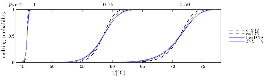
Figure 5: Average melting probability for random DNA (with different AT fractions) as a function of temperature at different channel diameters. For a fixed AT fraction, $p_{\rm AT}$, we find that smaller channel diameters leads to decreased melting temperatures and a broader transition (compare to Fig. 3). The main effect of the heterogeneity (non-zero $p_{\rm AT}$) is to further broaden the transition compared to melting of homo-DNA – the transition is broadest for the case $p_{\rm AT}=1/2$. Parameters: number of basepairs = $2\cdot 10^{5}$, and salt concentration = 0.01 $M$. Each curve is an average over 200 random sequences of length 200 kilo basepairs with a given AT-fraction, $p_{\rm AT}$. Note that ‘free DNA’ here refers to the case $c=1.5$ (unconfined ideal polymer).

In order to investigate how the sequence affects the melting transition, in this section we present numerical results for confined random DNA (for such a scenario no analytical predictions are available). In all simulations we generated 200 random sequences with a given AT-fraction, $p_{\rm AT}$, then used the Fixman-Freire approximation to predict a set of probability profiles. Finally, we calculated the average melting probability from this set.

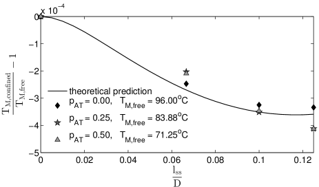
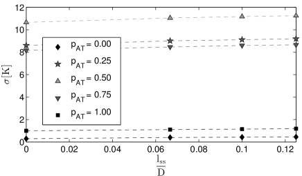
Figure 6: Confinement induced shift in melting temperature (units of Kelvin) and width of melting curves, for random DNA with AT fraction $p_{\rm AT}$ , as a function of inverse channel diameter. (Top) Shift of the melting temperature. Interestingly, the shift in melting temperature, Eqs. (23) and (24), obtained for a homo-DNA scenario, works rather well also for random DNA. (Bottom) Width of the melting curve. We notice that the width increases with decreasing channel diameter, and that the width is at maximum for $p_{\rm AT}=1/2$. Input parameters were the same as in Fig. 3.

In Fig. 5 we display the average melting probability for different channel diameters as a function of temperature for three different $p_{\rm AT}=\{0,0.25,0.5\}$. The results from Fig. 5 are further analyzed in Figure 6 which shows results for the melting temperature (top) and width (bottom) of the melting curve as a function of channel diameter. These results where obtained from melting curves as displayed in Fig. 5 in an identical fashion as in the previous subsection.

Figs. 5 and 6 show a number of interesting results. The main effect of the heterogeneity (non-zero $p_{\rm AT}$) is to further broaden the transition – the transition is broadest for the case $f_{\rm AT}=1/2$, and sharpest for homo-DNA, $p_{\rm AT}=1$ (pure AT) and $p_{\rm AT}=0$ (pure GC). Just as for the homo-cases (see previous subsection) we find, for a fixed value of $p_{\rm AT}$, that increasing confinement leads to a decreased melting temperature and an increase in the width of the transition. Interestingly, the shift in melting temperature, Eqs. (23) and (24), obtained for a homo-DNA scenario, works rather well also for random DNA, see Fig. 6 (top).

Studying Fig. 6 (Bottom) we see that while confinement broadens the melting transition also for random DNA, the effect is relatively small compared to the intrinsic width of the transition, which is much larger for random DNA compared to the homo-DNA case. This effect is also seen in Fig. 5, where we find that the difference between “free DNA” and confined random DNA is small.

IV.3 T4 phage DNA molecules

We now investigate a “real” DNA sequence - T4 phage, and compare to the melting behavior for random DNA.

In Fig. 7 we display the melting probability for free DNA and DNA confined to a channel with different diameters as a function of temperature for T4 phage and for random DNA with the same length $L=165643$ and AT ratio $p_{\rm{AT}}=0.64711$. Figures 8 (top, bottom) show the shift of the melting temperature and the change of the width $\sigma$ for different confinement.

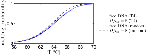
Figure 7: Melting probability for a T4 phage DNA, and random DNA, as a function of temperature at different channel diameters. The melting behavior of T4 phage DNA (same $p_{\rm AT}$ and number of basepairs as the T4 phage DNA sequence) is very similar to its associated random sequence melting curve. However, the random DNA melting curve is somewhat steeper. Parameters: number of basepairs = $168900$, and salt concentration = 0.01 $M$. Each random curve is an average over 200 random sequences with a given AT-fraction, $p_{\rm AT}=0.647016$. The sequence for T4 phage was downloaded from the NCBI GenBank (NC_000866.4).

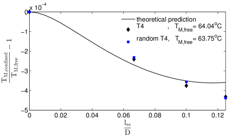
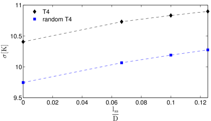
Figure 8: Shift in melting temperature and width of melting curves T4 phage DNA and associated random DNA (same AT fraction), see Fig. 7, as a function of inverse channel diameter. (Top) Change of the melting temperature (units of Kelvin)due to confinement, where the solid curve is Eqs. (23) and (24). Notice that the shift in melting temperature for T4 phage DNA is very similar to the melting temperature for a random DNA with the same AT fraction. (Bottom) Width of the melting curve at different confinement. The width of the melting curve for T4 phage DNA is slightly larger than the width for a random DNA with the same AT fraction. Input parameters were the same as in Fig. 7.

From Figures 7 and 8 a few things are worth pointing out. First, we notice that the melting curves for random DNA and T4 phage DNA are very similar. The main difference is that the width is somewhat increased for T4 DNA (however, less than 10 $\%$ for all channel diameters investigated). Obviously, these findings cannot be generalized to arbitrary “real” sequences, but shall, rather, be used as a motivation for why studying random DNA may be relevant also for DNA melting experiments.

V Summary and outlook

In this study we investigate how confinement affects the DNA melting transition. The statistical physics description of this process has a long history, and is commonly described in terms of the Poland-Scheraga (PS) model. The PS model is an Ising type model with heterogeneous interaction due to the sequence dependent energies required for breaking the bonds between the complementary bases. Moreover, including the configurational entropy associated with a melted DNA region gives rise to an effective long range interaction. It has been found previously that this loop entropy factor changes the nature of the DNA melting transition – from “smooth” in the absence of this factor, to first order when the loop factor is included.kafri These results pertain to a scenario of identical basepairs along an unconfined DNA.

Inspired by recent experiments,reisner2010 ; reisner2012 we calculate the effect that confinement in a nanochannel has on the melting transition of DNA. By subsequent numerical solutions of the PS model, and simplified arguments, we demonstrate that the confinement has three effects: the melting temperature is decreased, the confinement broadens the melting transition, and the shape of the melting curve goes from a functional form for unconfined melting (loop exponent $c=3/2$) to a form consistent with one-dimensional melting ($c=1/2$). We further quantify the sequence dependence of the melting transition, and find that the transition is broadest when the fraction of AT basepairs is 1/2. Relative to the width of the transition in the unconfined case, the broadening effect of confinement is smaller for random DNA than for homo-DNA. We also investigate “real” DNA, here T4 phage DNA, and find that its melting behavior is very similar to the melting of a random DNA with the same AT fraction. This finding gives further importance to recent efforts for understanding DNA melting of unconfined random DNA.hwa ; garel_04 ; giacomin2009 ; alexander2009 ; derrida2014

Throughout this study we use a functional form of the loop factor $g(m)$ for a confined chain, which is derived assuming ideal chain statistics (no self-exclusion effects included), and relaxing the constraint that within a melted region no complementary base pair binding must take place.werner_schad2015 While these approximations imply that one cannot expect the predictions of this study to be exactly valid for real DNA, we find a qualitatively similar effect of confinement upon the melting transition for simulations of an ideal DNA model and of a self-avoiding one in Ref. werner_schad2015, . We therefore expect that the results of this study furnish a qualitatively correct description of the effect of confinement on the melting transition of real DNA.

In a broader perspective, our study sheds light on the DNA strand separation in cells. The cell interior is a confined and crowded environment, where the crowding due to other macromolecules is known to affect vital biological processes such as the folding of proteins, diffusive transport and reaction rates.(Ellis_2003, ) Our study serves as a first step towards an understanding of how confinement and crowding affects the DNA melting, with potential implications for understanding of the processes whereby proteins access single strands of DNA,mark ; mark1 and for transcription initiationkalo ; yeramian in living cells.

VI Acknowledgment

TA is grateful to the Swedish Research Council for funding (grant no 2009-2924 and 2014-4305). BM acknowledges financial support by the Swedish Research Council and by the Göran Gustafsson Foundation for Research in Natural Sciences and Medicine.

Appendix A Numerical implementation

In this appendix we introduce one exact scheme, the Poland algorithm, and one approximate scheme, the Fixman-Freire approximation, for computing DNA melting profiles.

Let us first introduce some notation. The full sequence of basepairs enters via the position-dependence of the statistical weights

$$\alpha_{i}=\exp\{-E_{\rm hb}(i)/[RT]\}$$ (26)

for breaking the hydrogen-bonds of the basepair at position $i$, and

$$\delta_{i}=\exp\{-E_{\rm st}(i-1,i)/[RT]\}$$ (27)

for disrupting the stacking interactions between basepairs $i-1$ and $i$. In addition, we need the parameters $\xi$ and the loop factor $g(m)$, see main text.

A.1 The Poland algorithm

We now provide an exact scheme, the Poland algorithmpoland_algo for clamped ends, for computing the probability that basepair $k$ is open. The algorithm presented here extends previous methods by incorporating explicit stacking interactions: previous approaches “lumped” one Boltzmann factor of stacking interactions together with the $\xi$, giving rise to a cooperativity parameters, $\sigma_{0}$.

The Poland algorithm has two components. First, the conditional probability $P_{c}(k)$ that basepair $k+1$ is closed, provided that basepair $k$ is closed, is computed. Note that we here use the (somewhat funny) short-hand notation $P_{c}(k)=P_{c}(k+1|k)$ following Poland.poland_algo Secondly, the unconditional probability $P_{u}(k)$ that basepair $k$ is closed, is computed. In practice, however, one does not directly work with $P_{c}(k)$ but rather introduces $T_{k}=\alpha_{k}\delta_{k}P_{c}(k)$. If we now extend the algorithm from Ref. poland_algo, to the case of clamped boundary conditions and explicit stacking parameters, we find the following recursion relation:

$$T_{N} = \alpha_{N}\delta_{N},$$

$$T_{k} = \alpha_{k}\delta_{k}[1+\sum_{j=1}^{N-k}a_{k}(j)]^{-1},\ k=N-1,N-2,...,0,$$

where $a_{k}(j)\equiv q_{I}(k,j)\prod_{l=k+1}^{j+k}P_{c}(l)$ with the statistical weight $q_{I}(k,j)$ for a bubble with its left boundary at position $k$ (basepair $k$ is closed and basepair $k+1$ is open) and consisting of $j$ consecutive open basepairs:

$$q_{I}(k,j)=\xi g(j)\prod_{l=k+1}^{j+k}\alpha_{l}\prod_{l=k+1}^{j+k+1}\delta_{l}.$$ (29)

We above defined $\alpha_{0}=\delta_{0}=1$. The quantity $a_{k}(j)$ is conveniently computed using the recursion relation

$$a_{k}(1) = \xi g(1)\delta_{k+2}T_{k+1}\qquad k=0,1,...,N-1,$$

$$a_{k}(j) = \frac{g(j)}{g(j-1)}T_{k+1}a_{k+1}(j-1)\qquad j=2,...,N-k.$$

The (unconditional) probability $P_{u}(k)$ that basepair $k$ is then obtained from the equations:

$$P_{u}(0) = 1,$$

$$P_{u}(1) = T_{0},$$

$$P_{u}(k+1) = P_{u}(k)P_{c}(k)+\sum_{j=0}^{k-1}\mu_{k}(j)P_{u}(j),\ k=1,2,...,N.$$

We further define $\mu_{k}(j)=q_{I}(j,k-j)\prod_{l=j}^{k}P_{c}(l)$ from which we find the recursion relation:

$$\mu_{k}(k-1) = \xi g(1)\frac{\delta_{k+1}}{\alpha_{k-1}\delta_{k-1}}T_{k-1}T_{k}\qquad k=2,3,...,N,$$

$$\mu_{k}(j) = \frac{g(k-j)}{g(k-j-1)}\frac{\delta_{k+1}}{\delta_{k}}T_{k}\mu_{k-1}(j)$$ (32)

$$j=0,1,...,k-2.$$

The Poland algorithm for clamped DNA and explicit stacking parameters thus becomes: First use Eqs. (A.1) and (A.1) to obtain $T_{k}$ for $k=N,N-1,...,0$. Then use Eqs. (A.1) and (A.1) to obtain $P_{u}(k)$ for $k=0,1,.....,N+1$. A consistency check of the calculation is that $P_{u}(N+1)\equiv 1$ due to the clamping.

The mean number of bubbles used in appendix C.1 can easily be determined from $P_{u}(k)$ and $P_{c}(k)$ as the number of left boundaries (basepair $i$ closed, basepair $i+1$ open):

$$\langle N_{B}\rangle = \sum_{i}\langle s_{i}(1-s_{i+1})\rangle$$ (33)

$$= \sum_{i}P_{u}(i)-\sum_{i}P_{u}(i)P_{c}(i)$$

where we introduced the “spin” of a basepair: $s_{i}=1$ if basepair i is closed and $s_{i}=0$ otherwise.

The Poland algorithm scales with the number of basepairs $N$ as $N^{2}$. In practice, we therefore do not use the Poland algorithm for $N>10$ kbp. In the next section we present an algorithm whic scales linear in $N$, the Fixman-Freire approximation.fixman

A.2 Fixman-Freire approximation

The Fixman-Freire (FF) approximation uses the fact that a sum of exponentials is a good approximation for a power law function. The sums in Eqs. (A.1) and (A.1) give rise to the $N^{2}$ scaling of the Poland algorithm. Replacing the loop factor $g(m)$ (as part of both sums, see Eq. (29)) by a sum of exponentials with $I$ terms, reduces the scaling of the approximation to an $NI$-scaling.

Thus, within Fixman-Freire’s method, the following approximation is introduced:

$$g(m)\approx\sum_{i=1}^{I}c_{i}\exp(-b_{i}m)$$ (34)

. Applied on the sum in Eq. (A.1), we find

$$T_{k}=\alpha_{k}\delta_{k}[1+\sum_{i=1}^{I}c_{i}S_{i}(k)]^{-1}$$ (35)

and the recursion relation

$$S_{i}(N) = 0$$

$$S_{i}(k-1) = T_{k}\exp(-b_{i})[\xi\delta_{k+1}+S_{i}(k)].$$ (36)

Similarly, Eq. (A.1) becomes

$$P_{u}(k+1)=P_{u}(k)P_{c}(k)+\sum_{i=1}^{I}c_{i}A_{i}(k)$$ (37)

with recursion relation

$$A_{i}(0) = 0$$

$$A_{i}(k+1) = P_{c}(k+1)\alpha_{k+1}\delta_{k+1}\exp(-b_{i})$$ (38)

$$\left[\xi\delta_{k+1}P_{u}(k)P_{c}(k)+A_{i}(k)\right].$$

The coefficients $c_{i}$ and $b_{i}$ are determined from a fit on $2I$ points, $l_{i}$ (chosen such that the log’s are equally distributed on the domain where the approximation should be valid, i.e. from 1 to the total length of the DNA sequences). Starting with all coefficients set to zero, first the guess values $c_{I}$ and $b_{I}$ are determined from $g(l_{2I})$ and $g(l_{2I-1})$, then follow $c_{I-1}$ and $b_{I-1}$ using the new set of parameters and so on. If no convergence can be achieved, the parameters are determined for a larger interval, which is then slowly shrunk again with the new set of parameters as a first guess.

Appendix B DNA melting behavior for homo-DNA

In this appendix we analyze exact recursion relations for the partition function for the Poland-Scheraga model, and provide an analytic expression for the melting probability for homo-DNA.

Following Ref. garel_04, we divide the DNA molecule into a left region, i.e. basepairs $\{1,...,k-1\}$ and a right region, basepairs $\{k+1,...,N\}$, where $k$ varies. The end basepairs, basepairs number 0 and $N+1$, are here assumed clamped (closed). Garel and Orland, see Ref. garel_04, , proceed by deriving a recursion relation (see below) for the statistical weights (partition functions), $Q_{L}(k)$ and $Q_{R}$(k), for the “left” and “right” regions with the constraint that basepair $k$ is closed. Given $Q_{L}(k)$ and $Q_{R}(k)$ we can write most quantities of interest. In particular, the probability for having basepairs $k$ closed is simply

$$P(k)=1-\frac{Q_{L}(k)Q_{R}(k)}{Q_{L}(N+1)}.$$ (39)

Due to symmetry, recursion relations for $Q_{R}(k)$ are of the same form as those for $Q_{L}(k)$. We therefore now limit ourselves to studying $Q_{L}(k)$. We further find it convenient to rescale $Q_{L}(k)$ as

$$q_{L}(k) \equiv \frac{Q_{L}(k)}{\beta_{1}\beta_{2}\cdots\beta_{k}},$$ (40)

where $\beta_{k}=\alpha_{k}\delta_{k}$ with $\alpha_{k}$ and $\beta_{k}$ defined in Eqs. (26) and (27). In terms of these rescaled statistical weights, the Garel-Orland recursion relationgarel_04 becomes:

$$\beta_{k+1}q_{L}(k+1)=q_{L}(k)+\sigma_{0,k+1}\sum_{j=0}^{k-1}g(k-j)q_{L}(j)$$ (41)

for $k=1,...,N$. We above introduced the local cooperativity parameter $\sigma_{0,k}=\xi\delta_{k}$. The “boundary” conditions are $q_{L}(0)=1$ and $q_{L}(1)=1/\beta_{1}$. We note that, in principle, the recursion relation above can be used to predict DNA melting curves. However, the quantity $q_{L}(k)$ typically “explodes” exponentially with the number of basepairs. Therefore, two alternative numerical methods, the Poland algorithm and the Fixman-Freire approximation, are described in appendix A.

Let us consider the case of homo-DNA, i.e. when the basepair energies are the same along the DNA. We then set $\beta_{k}=\beta$ and $\sigma_{0,k}=\sigma_{0}$ in Eq. (41). We notice that the last term in Eq. (41) has the form of a convolution (if we add the term $j=k$ to the sum). We therefore introduce the generating function (if we replace $z\rightarrow 1/z$ below we get a $z$-transform)

$$\bar{q}_{L}(z)=\sum_{k=0}^{\infty}q_{L}(k)z^{k}$$ (42)

which, after using the convolution theorem for $z$-transforms and some rearrangements (for convenience we also define $g(0)\equiv 0$), gives the solution to Eq. (41) as:

$$\bar{q}_{L}(z)=\frac{1}{1-\beta^{-1}z[1+\sigma_{0}\bar{g}(z)]},$$ (43)

where

$$\bar{g}(z)=\sum_{k=1}^{\infty}g(k)z^{k}$$ (44)

For the case $g(k)=k^{-c}$ we have that $\bar{g}(z)={\rm Li}_{c}(z)$ is the polylogarithmic function. It is noteworthy that analytic continuation of the polylogarithmic function to the complex plane has a branch cut for ${\rm Re}\ z>1$. The generating function $\bar{q}_{L}(z)$ therefore also has a branch cut in the same domain.

In order to invert the exact result for the generating function, Eq. (43), we note, see Eq. (42), that $q_{L}(k)$ is the $k$:th term in a series expansion in $z$, i.e.,

$$q_{L}(k)=\frac{1}{k!}\frac{d^{k}\bar{q}_{L}(z)}{dz^{k}}|_{z=0}=\frac{1}{2\pi i}\oint_{C}\frac{\bar{q}_{L}(z)}{z^{k+1}}dz$$ (45)

where the last equality is a standard result in complex analysis.wunsch The integration above is over a closed contour $C$ around $z=0$, see Fig. 9.

Figure 9: Contours used for solving the Poland-Scheraga model analytically for homo-DNA. Integration along the black circle around $z=0$ gives the statistical weight $q_{L}(k)$ through Eqs. (43) and (45). The blue contours depict a useful deformation of the black contour: We deform the contour to “infinity”. When deforming the original contour, we “pass” the pole at $z=z_{0}$, which must be subtracted (notice the “negative” orientation of the contour around $z=z_{0}$). The contour along ${\rm Re}\ z=[1,\infty]$ is needed for the case of a power law form for the loop factor, as the associated $z$-transform (polylogarithmic function) has a branch cut there.

Following Ref. Wiegel, the contour integral in Eq. (45) is evaluated by deforming the original contour as described in Fig. 9. The deformed contour has several parts. One of these parts is a contour around the pole $z_{0}$ of $\bar{q}_{L}(z)$, and, in fact, the thermodynamic behavior is determined by the contribution from this pole.Wiegel For large $k$ we therefore have

$$q_{L}(k)\sim\frac{1}{2\pi i}\oint_{C_{0}}\frac{\bar{q}_{L}(z)}{z^{k+1}}dz$$ (46)

where $C_{0}$ is the contour around the pole depicted in Fig. 9. The pole, $z_{0}$, is determined by the condition $\bar{q}_{L}(z_{0})=0$, i.e.,

$$\bar{g}(z_{0})=\frac{\beta-z_{0}}{\sigma_{0}z_{0}}$$ (47)

where we used Eq. (43). So, using the Cauchy theoremwunsch we have:

$$q_{L}(k)\sim-{\rm Res}[\frac{z^{-k-1}}{1-\beta^{-1}z[1+\sigma_{0}\bar{g}(z)]},z=z_{0}]$$ (48)

where ${\rm Res}[...]$ denotes the residue. Using the fact thatwunsch ${\rm Res}[A(z)/B(z),z=z_{0}]=A(z_{0})/B^{\prime}(z_{0})$ if $z_{0}$ is a simple pole and $A(z)$ is a regular function, we find:

$$q_{L}(k)=\frac{\beta z_{0}^{-k-1}}{1+\sigma_{0}[\bar{g}(z_{0})+z_{0}\bar{g}^{\prime}(z_{0})]}.$$ (49)

This result holds provided that $z_{0}\in[0,1]$; if $z_{0}\geq 1$ then the pole is in a branch cut (for a power-law form of $g(m)$), see Fig. 9, and does not contribute to $q_{L}(k)$. Finally, we simplify the results above using Eq. (47), and combining with Eq. (40) we find the partition function:

$$q_{L}(k)\sim\frac{z_{0}^{-k}}{1+\sigma_{0}z_{0}\beta^{-1}\bar{h}(z_{0})}$$ (50)

where we defined the function: $\bar{h}(z)=z\bar{g}^{\prime}(z)$. Eq. (50) is our final expression for the rescaled partition function for the Poland-Scheraga model for homo-DNA melting in the thermodynamic limit. For the general case we evaluate $\bar{g}(z)$ using the definition, Eq. (44). Using this same definition, we find that

$$\bar{h}(z)=\sum_{k=1}^{\infty}kg(k)z^{k}$$ (51)

thereby providing an explicit expression for all quantities in Eq. (50).

Finally, by combining Eqs. (39), (40), and (50), we obtain our final expression for the melting probability:

$$P=1-\frac{1}{1+\sigma_{0}\beta^{-1}z_{0}\bar{h}(z_{0})}$$ (52)

where $\bar{g}(z)$ is given in Eq. (44) and $\bar{h}(z)$ in Eq. (51). These expressions can be used to numerically evaluate $\bar{g}(z)$ and $\bar{h}(z)$ by replacing the series by sums. The quantity $z_{0}$ is determined by (numerically) solving Eq. (47). Thus, the equations given here provide means for straightforward calculation of the melting probability for different choices of $g(m)$ in the thermodynamic limit. For the case $g(k)=k^{-c}$ we have $\bar{g}(z)={\rm Li}_{c}(z)$ and $\bar{h}(z)={\rm Li}_{c-1}(z)$, where ${\rm Li}_{c}(z)$ is the polylogarithmic function.

Appendix C Analysis of melting curve for unconfined DNA

This appendix provides results for melting curves of unconfined DNA, and, thus, serves a background to the main text, where melting of confined DNA molecules is studied.

C.1 Deviation from the Marmur-Doty melting temperature

The Marmur-Doty formula, Eq. (4), is based on a simple estimate where one assumes melting to occur at a temperature where the free energy for breaking one hydrogen bond and one stacking interaction equals zero. Due to, for instance, neglect of the “boundary energy” $(1/2)RT\log\xi$ and the loop factor $g(m)$, which favors smaller bubbles, Eq. (4) is only an approximation.

In order to estimate shifts in melting temperature compared to the Marmur-Doty formula for unconfined DNA, we note that an entropic contribution $R\log\xi$ has to be assigned to each bubble. The corrected melting temperature can then be estimated from the number of bubbles, $N_{B}$, as

$$T_{\rm{M}}^{\rm B}=\frac{\sum H}{\sum S}=\frac{S_{\rm{ref}}}{S_{\rm{ref}}-R\log\xi\frac{N_{\rm B}}{N}}T_{\rm M}$$ (53)

In practice, we further replace $N_{B}$ by its expected number of bubbles $\langle N_{B}\rangle$. In Figure 10 we tested the above mean-field prediction in the following way: using the Fixman-Freire approximation we determined the shift in melting temperature from the Marmur-Doty formula for a range of $p_{\rm AT}$ and loop exponents $c$. Simultaneously, we determined the expected number of bubbles, $\langle N_{B}\rangle$, see Section A for details. From Figure 10 we notice that, while Eq. (53) captures the typical behavior for the shift as a function of number of bubbles, there are deviations. For $c\geqslant 1$, there is clear relation between the number of bubbles and the deviation from the Marmur-Doty melting temperature. For larger values of $c$, however, the trend is less pronounced. A possible explanation for this “large $c$” effect is that while the curves get wider with smaller values of $c$, the asymmetry of the melting transition results in the point $T(f=0.5)$ to be shifted to smaller temperatures.

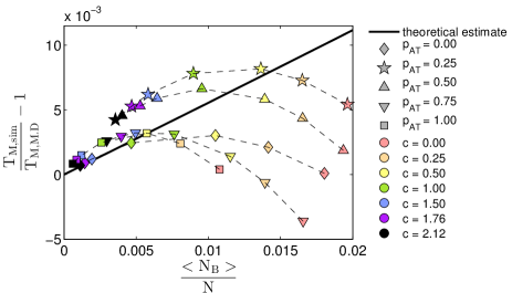
Figure 10: Shift of the simulated melting temperature $T_{\rm{M,sim}}$ (units of Kelvin) compared to the Marmur-Doty melting temperature $T_{\rm{M,M.D.}}$ as a function of the simulated mean number of boundaries at $T_{\rm{M,sim}}$ at $T_{\rm{M,sim}}$ for random unconfined DNA. The solid line shows our theoretical estimate from Eq. (53). For $c\geqslant 1$, there is clear relation between the number of bubbles and the deviation from the Marmur-Doty melting temperature. For larger values of $c$, however, we find less correlation between the shift in melting temperature and $\langle N_{B}\rangle$. Averages are taken over 200 different sequences of length $2\cdot 10^{5}$ basepairs at AT ratios $p_{\rm{AT}}={0,0.25,0.5,0.75,1}$ (different markers), each for different loop exponents $c={2.12,1,76,1.5,0.5,0}$ (indicated by different colors).

Notice that we in the main text avoid “problems” with the Marmur-Doty formula by always using simulated melting temperatures as reference.

A final word of caution is here in order. The hydrogen bond energies we use in the simulations are not measured for individual base-pairs, but estimated from global melting of a few model sequences and therefore already contain the contribution of the ring factor. We therefore get too large temperatures from our simulations already for unconfined DNA with $c=2.12$, where the Marmur-Doty relation was found experimentally.owen ; FK For smaller values of c (or smaller channels), the melting transition gets broader and the mean number of bubbles at $T_{M}$ increases.

C.2 Width of the melting transition as a function of loop exponent c

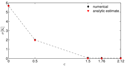
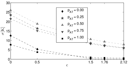
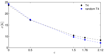
Figure 11: Width of the melting curve as a function of the loop exponent $c$ for unconfined homo-DNA (top), unconfined random DNA (middle) and unconfined T4-phage DNA (bottom) (with associated random DNA, same AT fraction). Parameters are the same as in Fig. 5.

Figure 11 shows the change of the width $\sigma$ for different loop exponents c for unconfined DNA. The width was extracted using the same approach as described in subsection IV.1. We find that increasing $c$ decreases the width of the transition as it should. These findings hold for the three cases of interest here: 1. homo-DNA, 2. random DNA for different AT fractions, and 3. T4 phage DNA. The prefactors for the width are larger for case 2. than for case 1. The homo-DNA case does not give identical results to the $f_{\rm AT}=0$ and $f_{\rm AT}=1$ cases due to the additional different stacking parameters for the latter cases as compared to the homo-DNA case, see section II.2.

C.3 Analytical prediction for different loop exponents c

Figure 12 shows the melting probability for unconfined homo-DNA for different values of the loop exponent $c$, both using the numerical Poland algorithm and the analytic prediction introduced in section B. As before, we used Eq. (52), where $z_{0}$ was numerically obtained by solving Eq. (47). We find very good agreement between the numerical and analytical result. Note, however, that due to the finite size of the DNA sequences the numerical result for $c=1.5$ deviates slightly from the analytical result, which is obtained for the thermodynamic limit.

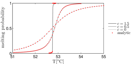
Figure 12: Melting probability as a function of temperature for an unconfined homo DNA for different loop exponents. The numerical results for a sequence of length 50 kilo basepairs (solid lines) are compared to the analytic prediction in the thermodynamic limit (red marks). We used $\xi=10^{−3}$ and melting temperature for a sequence ‘A … A’, see Eq. (6).

References

- (1) J.D. Watson and F.H.C. Crick F H C Cold Spring Harbor Symposia on Quantitative Biology 18, 123 (1953).
- (2) B. Alberts, D. Bray, K. Hopkin, A. Johnson, J. Lewis, M. Raff, K. Roberts, and P. Walter Essential cell biology, Garland Science, 2013.
- (3) D. Poland D and H. Scheraga, Theory of Helix-Coil Transitions in Biopolymers, Academic Press, New York (1970).
- (4) M. Guéron, M. Kochoyan M and J.-L. Leroy, Nature 328, 89 (1987).
- (5) E. Yeramian, Gene 255, 139 (2000); ibid. p. 151.
- (6) J. SantaLucia Jr, Proc. Natl. Acad. Sci. 95, 1460 (1998).
- (7) M.D. Frank-Kamenetskii, and S. Prakash, Physics of life reviews 11, 153 (2014).
- (8) R.M. Wartell R M and A.S. Benight, Phys. Rep. 126 67 (1985).
- (9) R.D. Blake, J.W. Bizzaro, J.D. Blake, G.R. Day, S.G. Delcourt, J. Knowles, K.A. Marx and J. SantaLucia Jr., Bioinformatics 15 370 (1999).
- (10) R. Blossey and E. Carlon, Phys. Rev. E 68, 061911 (2003).
- (11) M. Peyrard and A.R. Bishop, Phys. Rev. Lett. 62, 2755-2758; Dauxois T, Peyrard M & Bishop A R (1993) Phys. Rev. E 47, R44 (1989).
- (12) G. Kalosakas, K. Ø. Rasmussen, A.R. Bishop, C.H. Choi, A. Usheva, Europhys. Lett. 68, 127 (2004); C.H. Choi, G. Kalosakas, K. Ø. Rasmussen, M. Hiromura, A.R. Bishop, A. Usheva, Nucleic Acids Res. 32, 1584 (2004).
- (13) A. Krueger, E. Protozanova, and M.D. Frank-Kamenetskii, Biophys. J. 90, 3091 (2006); E. Protozanova, P. Yakovchuk and M.D. Frank-Kamenetskii, J. Mol. Biol. 342, 775 (2004).
- (14) M.E. Fisher, J. Stat. Phys. 34, 667 (1984), Sec. VI.
- (15) F.W. Wiegel, Conformational Phase Transition in a Macromolecule: Exactly Solvable models, in Phase Transitions and Critical Phenomena, vol. 7 Domb & Lebowitz (Editors).
- (16) Y. Kafri, D. Mukamel, and L. Peliti, Phys. Rev. Lett. 85, 4988 (2000).
- (17) T. Hwa, E. Marinari, K. Sneppen and L.-H. Tang L-H, Proc. Natl. Acad. Sci. USA 100, 4411 (2003).
- (18) T. Garel and H. Orland, Biopolymers 75, 453 (2004).
- (19) G. Giacomin, In Spin Glasses: Statics and Dynamics, pp. 235-270. Birkhäuser Basel (2009).
- (20) K.S. Alexander, and N. Zygouras, Comm. Math. Phys. 291 659 (2009).
- (21) B. Derrida, and M. Retaux, J. Stat. Phys. 156, 268 (2014).
- (22) B. Derrida and H.J. Hilhurst, J. Phys. A 16, 2641 (1983).
- (23) M. Ya. Azbel, Biopolymers 19, 61 (1980).
- (24) M. Ya. Azbel, Biopolymers 19, 81 (1980).
- (25) M. Ya. Azbel, Biopolymers 19, 95 (1980).
- (26) I.M. Lifshitz, Zh. Eksp. Teor. Fiz 65 1100 (1973).
- (27) H. Li, Z. Wang, N. Li, X. He and H. Liang, J. Chem. Phys. 141, 044911 (2014).
- (28) E. Werner, M. Reiter-Schad, T. Ambjörnsson and B. Mehlig, arXiv:1504.03082 [physics.bio-ph] (2015).
- (29) W. Reisner, N.B. Larsen, A. Silahtaroglu, A. Kristensen, N. Tommerup, J.O. Tegenfeldt, and H. Flyvbjerg, Proc. Nat. Acad. Sci. USA 107, 13294 (2010).
- (30) W. Reisner, J.N. Pedersen, and R.H. Austin, Rep. Prog. Phys. 75, 106601 (2012).
- (31) G. Altan-Bonnet, A. Libchaber and O. Krichevsky, Phys. Rev. Lett. 90, 138101 (2003).
- (32) T.Ambjörnsson, S.K. Banik, O. Krichevsky and R. Metzler, Phys. Rev. Lett. 97, 128105 (2006).
- (33) K. Pant, R. L. Karpel, and M. C. Williams, J. Mol. Biol. 327, 571 (2003).
- (34) I.M. Sokolov, R. Metzler, K. Pant, and M.C. Williams, Biophys. J. 89, 895 (2005); Phys. Rev. E 72, 041102 (2005).
- (35) C. H. Choi et al, Nucl. Acids Res. 32, 1584 (2004); G. Kalosakas et al, Europhys. Lett. 68, 127 (2004).
- (36) M. Fixman M and J.J. Freire, Biopol. 16, 2693 (1997).
- (37) See C. Richard and A.J. Guttmann, J. Stat. Phys. 115, 925 (2004) and Refs. therein.
- (38) A.R. Khokhlov and A. Yu Grosberg, Statistical physics of macromolecules Amer. Inst. of Physics (1994).
- (39) W. Reisner, J.N. Pedersen, and R.H. Austin, Rep. Prog. Phys. 75, 106601 (2012).
- (40) E. Werner, F. Westerlund, J.O. Tegenfeldt, B. Mehlig, Macromolecules 46, 6644 (2013).
- (41) D.R. Tree, Y. Wang, and K.D. Dorfman, Phys. Rev. Lett. 110 208103 (2013).
- (42) H.S. Carslaw and J.C. Jaeger, Conduction of heat in solids. Vol. 2. Oxford: Clarendon Press (1959).
- (43) P.-G. de Gennes, Scaling concepts in polymer physics, Cornell University Press (1979).
- (44) R.J. Ellis and A.P. Milton, Cell biology: Join the crowd, Nature 425, 27 (2003).
- (45) D. Poland, Biopolymers 13, 1859 (1974).
- (46) D.A. Wunsch, Complex Variables with Applications, 3rd ed., Pearson (2004).
- (47) R.J. Owen, L.R. Hill, and S.P.Lapage, Biopolymers 7, 503 (1969).