On the Splash Singularity for the free-surface of a Navier-Stokes fluid

Abstract.

In fluid dynamics, an interface splash singularity occurs when a locally smooth interface self-intersects in finite time. We prove that for $d$-dimensional flows, $d=2$ or $3$, the free-surface of a viscous water wave, modeled by the incompressible Navier-Stokes equations with moving free-boundary, has a finite-time splash singularity. In particular, we prove that given a sufficiently smooth initial boundary and divergence-free velocity field, the interface will self-intersect in finite time.

1. Introduction

1.1. The interface splash singularity

The fluid interface splash singularity was introduced by Castro, Córdoba, Fefferman, Gancedo, & Gómez-Serrano in [8] in the context of the one-phase water waves problem. As shown in Figure 1.1, A splash singularity occurs when a fluid interface remains locally smooth but self-intersects in finite time. Using methods from complex analysis together with a clever transformation of the equations, Castro, Córdoba, Fefferman, Gancedo, & Gómez-Serrano [8] showed that a splash singularity occurs in finite time for the water waves equations. In Coutand & Shkoller [16], we showed the existence of a finite-time splash singularity for the one-phase incompressible Euler equations with free-boundary using a very different approach, founded upon an approximation of the self-intersecting fluid domain by a sequence of smooth fluid domains, each with non self-intersecting boundary. For one-phase flow, it is the vacuum state on one side of the interface which permits this finite-time interface self-intersection, and neither surface tension nor magnetic fields nor other inviscid regularizations of the interface change this fact [7, 16], and even stationary solutions, having a splash singularity, have been shown to exist (see Córdoba, Enciso, & Grubic [10]).

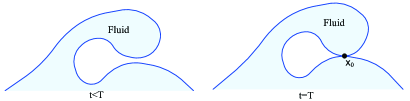
Figure 1.1. The splash singularity at a point $x_{0}$ occurs when a locally smooth interface self-intersects in finite time $t=T$.

On the other hand, for the two-phase incompressible Euler equations, wherein the moving interface is a vortex sheet, it was proven by Fefferman, Ionescu, & Lie [19] and Coutand & Shkoller [17] that a splash singularity cannot occur in finite-time while the interface remains locally smooth. In particular, there is a fundamental difference in the behavior of the fluid interface when vacuum is replaced with fluid in the mathematical model.

Since these results have been established for inviscid flows, it is natural to ask if splash singularities can occur for viscous flows modeled by the incompressible Navier-Stokes equations with a moving free-surface. Because the methods of constructing splash singularities for inviscid flows have relied on the ability to flow backward-in-time, a new strategy must be devised to study the parabolic Navier-Stokes equations. By using the change-of-variables employed in [8] together with stability estimates, Castro, Córdoba, Fefferman, Gancedo, & Gómez-Serrano in [9] have shown the existence of finite-time splash singularities for the Navier-Stokes equations. Herein, we give a different proof which is amenable to any space dimension $d\geq 2$.

1.2. The Eulerian description of the Navier-Stokes free-boundary problem

For $0\leq t\leq T$, the evolution of a $d$-dimensional ($d=2$ or $3$) one-phase, incompressible, viscous fluid with a moving free boundary is modeled by the incompressible Navier-Stokes equations:

$$u_{t}+u\cdot\nabla u+\nabla p =\nu\Delta u\ \ \ \text{in}\ \ \Omega(t)\,,$$ (1.1a)

$${\operatorname{div}}u =0 \text{in}\ \ \Omega(t)\,,$$ (1.1b)

$$\nu\operatorname{Def}u\cdot n-p\,n =0\ \ \text{on}\ \ \Gamma(t)\,,$$ (1.1c)

$$\mathcal{V}(\Gamma(t)) =u\cdot n$$ (1.1d)

$$u =u_{0}\ \ \text{on}\ \ \Omega(0)\,,$$ (1.1e)

$$\Omega(0) =\Omega_{0}\,.$$ (1.1f)

The open subset $\Omega(t)\subset\mathbb{R}^{d}$, $d=2$ or $3$, denotes the time-dependent volume occupied by the fluid, $\Gamma(t):=\partial\Omega(t)$ denotes the moving free-surface, $\mathcal{V}(\Gamma(t))$ denotes normal velocity of $\Gamma(t)$, and $n(t)$ denotes the exterior unit normal vector to the free-surface $\Gamma(t)$. The vector-field $u=(u_{1},..,u_{d})$ denotes the Eulerian velocity field, and $p$ denotes the pressure function. We use the notation $\nabla=(\partial_{1},...,\partial_{d})$ to denote the gradient operator, and set $\operatorname{Def}u=\nabla u+\nabla u^{T}$, twice the symmetric part of the gradient of velocity. We have normalized the equations to have all physical constants equal to 1.

The pressure $p$ is a solution to the following Dirichlet problem:

$$-\Delta p =u^{i},_{j}u^{j},_{i}\ \ \ \text{in}\ \ \Omega(t)\,,$$ (1.2a)

$$p =n\cdot\left[\nu\operatorname{Def}u\cdot n\right]\ \ \text{on}\ \ \Gamma(t)\,,$$ (1.2b)

so that given an initial domain $\Omega$ and an initial velocity field $u_{0}$, the initial pressure is obtained as the solution of (1.2) at $t=0$.

Definition 1.1.

Given a locally smooth, time-dependent fluid interface or free-boundary, if there exists a time $T<\infty$ such that the interface $\Gamma(T)$ self-intersects at a point while remaining locally smooth, we call this point of self-intersection at time $T$ a “splash” singularity.

We prove that there exist smooth initial data for the Navier-Stokes equations (1.1) for which such a splash singularity occurs in finite time.

1.3. Statement of the Main Theorem

Theorem 1.1 (Finite-time splash singularity).

There exist

1. open bounded $C^{\infty}$-class initial domains $\Omega\subset\mathbb{R}^{d}$, $d=2$ or $3$, with $N$ denoting the unit normal vector field on $\partial\Omega$, and

2. smooth divergence-free velocity fields $u_{0}$ satisfying the compatibility condition

   $$\left[\operatorname{Def}u_{0}\cdot N\right]\times N=0\text{ on }\partial\Omega\,,$$

such that after a finite time $T^{*}>0$, the solution to the Navier-Stokes equations (1.1) has a splash singularity; that is, the interface $\Gamma(T^{*})$ self-intersects.

In Theorem 10.1, we show that the geometry of such a splash singularity can be prescribed arbitrarily close (in the $H^{3}$ norm) to any sufficiently smooth and prescribed self-intersecting domain.

1.4. Prior results for the incompressible Navier-Stokes equations with moving free-surface

Local-in-time well-posedness of solutions to (1.1) have been known since the pioneering work of Solonnikov [27, 28, 29]; his proof did not rely on energy estimates, but rather on Fourier-Laplace transform techniques, which required the use of exponentially weighted anisotropic Sobolev-Slobodeskii spaces with only fractional-order spatial derivatives for the analysis. Beale [5] proved local well-posedness in a similar functional framework, and Abels [1] established the existence theory in the $L^{p}$ Sobolev space framework. Well-posedness in energy spaces was established by Coutand & Shkoller in [12] for the case of surface tension on the free-boundary, and for Navier-Stokes fluid-structure interaction problems wherein a viscous fluid is coupled to an elastic solid, in [13, 14]. Guo & Tice [23] also used energy spaces for local well-posed for the case of zero surface tension.

Beale [6] established global existence of solutions to (1.1) for small perturbations of equilibrium. More recent small-data global existence and decay results (both with and without surface tension) can be found in [31], [26], [25], [20], [4], and [21, 22]. Recent results on the limit of zero viscosity and the limit of zero surface tension can be found in [24], [18], and [32].

For the history of the well-posedness and singularity theory for the inviscid problem, we refer the reader to the introduction in [15] and [17].

1.5. Outline of the paper

In Section 2, we define our notation. In Section 3, we define a sequence of domains $\Omega^{\epsilon}$ that we use as the initial data for the splash singularity, wherein the boundary $\Gamma^{\epsilon}$ of these domains is close to self-intersection with a distance $\epsilon$ between two approaching portions of $\Gamma^{\epsilon}$. We convert the Navier-Stokes equations to Lagrangian coordinates in Section 4, thus fixing the domain. In Section 5, we present some preliminary lemmas which show that the constant appearing in elliptic estimates and the Sobolev embedding theorem is independent of $\epsilon$. In Section 6, we define the sequence of initial divergence-free velocity fields that are guaranteed to satisfy the single compatibility condition that we require, and whose norm is independent of $\epsilon$. Section 7 is devoted to the basic a priori estimates for the Navier-Stokes equations in Lagrangian coordinates; following our approach in [12], we establish estimates for velocity $v\in L^{2}(0,T;H^{3}(\Omega^{\epsilon}))\cap C^{0}([0,T];H^{2}(\Omega^{\epsilon}))$ which are independent of $\epsilon$. We then prove that the vertical component of velocity $v(\cdot t)$ at time $t$ remains in an $O(t^{\frac{1}{4}})$ neighborhood of the vertical component of the initial velocity field. Using this fact, we prove the main theorem in Section 8; we show that by choosing $\epsilon$ appropriately, a finite-time splash singularity must occur at some time $T^{*}\in(0,10\epsilon)$. We consider a completely arbitrary geometry for a splash singularity in Section 9, by following our definition of a generalized splash domain from our previous work in [16]. This, then, allows us to show in Section 10, that we can construct a splash singularity for a geometry which is arbitrarily close in $H^{3}$ to any prescribed $H^{3}$ splash domain.

2. Notation, local coordinates, and some preliminary results

2.1. Notation for the gradient vector

Throughout the paper the symbol $\nabla$ will be used to denote the $d$-dimensional gradient vector $\nabla=\left(\frac{\partial}{\partial x_{1}}\,,\frac{\partial}{\partial x_{2}}\,,...,\,\frac{\partial}{\partial x_{d}}\right)$.

2.2. Notation for partial differentiation and the Einstein summation convention

The $k$th partial derivative of $F$ will be denoted by $F,_{k}=\frac{\partial F}{\partial x_{k}}$. Repeated Latin indices $i,j,k$, etc., are summed from $1$ to $d$, and repeated Greek indices $\alpha,\beta,\gamma$, etc., are summed from $1$ to $d$$-$$1$. For example, $F,_{ii}=\sum_{i=1}^{d}\frac{\partial^{2}F}{\partial x_{i}\partial x_{i}}$, and $F^{i},_{\alpha}I^{\alpha\beta}G^{i},_{\beta}=\sum_{i=1}^{d}\sum_{\alpha=1}^{d-1}\sum_{\beta=1}^{2}\frac{\partial F^{i}}{\partial x_{\alpha}}I^{\alpha\beta}\frac{\partial G^{i}}{\partial x_{\beta}}$.

2.3. Tangential (or horizontal) derivatives

On each boundary chart $U_{l}\cap\Omega$, for $1\leq l\leq K$, we let $\bar{\partial}$ denote the tangential derivative whose $\alpha$th-component given by

$$\bar{\partial}_{\alpha}f=\left(\frac{\partial}{\partial x_{\alpha}}[f\circ\theta_{l}]\right)\circ\theta_{l}^{-1}=\left((\nabla f\circ\theta_{l})\frac{\partial\theta_{l}}{\partial x_{\alpha}}\right)\circ\theta_{l}^{-1}\,.$$

For functions defined directly on $B^{+}$, $\bar{\partial}$ is simply the horizontal derivative $\bar{\partial}=(\partial_{x_{1}},...,\partial_{x_{d-1}})$.

2.4. Sobolev spaces

For integers $k\geq 0$ and a bounded domain $U$ of $\mathbb{R}^{3}$, we define the Sobolev space $H^{k}(U)$ $(H^{k}(U;\mathbb{R}^{3}))$ to be the completion of $C^{\infty}(\bar{U})$ $(C^{\infty}(\bar{U};\mathbb{R}^{3}))$ in the norm

$$\|u\|_{k,U}^{2}=\sum_{|a|\leq k}\int_{U}\left|\nabla^{a}u(x)\right|^{2},$$

for a multi-index $a\in\mathbb{Z}^{3}_{+}$, with the convention that $|a|=a_{1}+a_{2}+a_{3}$. When there is no possibility for confusion, we write $\|\cdot\|_{k}$ for $\|\cdot\|_{k,U}$. For real numbers $s\geq 0$, the Sobolev spaces $H^{s}(U)$ and the norms $\|\cdot\|_{s,U}$ are defined by interpolation. We will write $H^{s}(U)$ instead of $H^{s}(U;\mathbb{R}^{d})$ for vector-valued functions.

2.5. Sobolev spaces on a surface $\Gamma$

For functions $u\in H^{k}(\Gamma)$, $k\geq 0$, we set

$$\|u\|_{k,\Gamma}^{2}=\sum_{|a|\leq k}\int_{\Gamma}\left|\bar{\partial}^{a}u(x)\right|^{2},$$

for a multi-index $a\in\mathbb{Z}^{2}_{+}$. For real $s\geq 0$, the Hilbert space $H^{s}(\Gamma)$ and the boundary norm $|\cdot|_{s}$ is defined by interpolation. The negative-order Sobolev spaces $H^{-s}(\Gamma)$ are defined via duality. That is, for real $s\geq 0$, $H^{-s}(\Gamma)=H^{s}(\Gamma)^{\prime}$.

2.6. The unit normal and tangent vectors

We let $n(\cdot,t)$ denote the outward unit normal vector to the moving boundary $\Gamma(t)$. When $t=0$, we let $N_{\epsilon}$ denote the outward unit normal to $\Gamma^{\epsilon}$. For each $\alpha=1,...,d-1$ and $x\in\Gamma^{\epsilon}$ , $\tau_{\alpha}(x)$ denotes an orthonormal basis of the ($d$$-$$1$)-dimensional tangent space to $\Gamma^{\epsilon}$ at the point $x$.

3. The sequence of initial domains $\Omega^{\epsilon}$

We shall use, as initial data, a sequence of domains, whose two-dimensional cross-section resembles a dinosaur neck arching over its body.

3.1. The “dinosaur wave” domains

Definition 3.1 (The domain $\Omega$).

Let $\Omega\subset\mathbb{R}^{d}$, $d=2,3$, be a smooth bounded domain (as shown on the left of Figure 3.1) with boundary $\Gamma$. We assume that there are three particular open subsets of $\Omega$ as follows:

1. There exists an open subset $\omega\subset\Omega$ such that its boundary $\partial\omega\subset\Gamma$ is a vertical circular cylinder of radius $r$ and of length $h>0$.

2. There exists an open subset $\omega_{+}\subset\Omega$ which is the lower-half of an open ball of radius $1$, located directly below the cylindrical region $\omega$, and in contact with the cylindrical region $\overline{\omega}$. The “south pole” of $\omega_{+}$ is the point $X_{+}$ (see Figure 6.1).

3. There exists an open subset $\omega_{-}\subset\Omega$ directly below, at a distance $1$, from the “south pole” $X_{+}$ of $\omega_{+}$, such that the points with maximal vertical coordinate in $\partial\omega_{-}\cap\Gamma$ form a subset of the horizontal plane $x_{d}=0$.

4. Coordinates are assigned to subsets of $\Omega$ as follows:

   1. The origin of $\mathbb{R}^{d}$ is contained in $\partial\omega_{-}\subset\Gamma\cap\{x_{d}=0\}$.

   2. The point $X_{+}$, the “south pole” of $\omega_{+}$, has the coordinates $X^{\alpha}_{+}=0$ for $\alpha=1,...,d-1$ and $X_{+}^{d}=1$.

   3. The top boundary of the hemisphere $\omega_{+}$ is the set $\{(x_{h},x_{d})\in\mathbb{R}^{d}\ :\ x_{d}={\frac{3}{2}},\ |x_{h}|<1\}$.

   4. The cylindrical region $\omega$ is given by $\{(x_{h},x_{d})\in\mathbb{R}^{d}\ :\ {\frac{3}{2}}<x_{d}<{\frac{3}{2}}+h,\ |x_{h}|<1\}$.

Figure 3.1. Left. The “dinosaur wave” domain $\Omega$ with boundary $\Gamma$. Right. The sequence of “dinosaur waves” $\Omega^{\epsilon}$ with boundary $\Gamma^{\epsilon}$, $\epsilon>0$, used as initial data for the Navier-Stokes splash singularity. In order to ensure that a splash occurs, the “dinosaur neck” $\omega^{\epsilon}$ stretches downward so that there is a distance $\epsilon$ between the two portions. The domains $\Omega^{\epsilon}$ simply stretch the neck of the dinosaur, and are identical to $\Omega$ away from the neck.

Definition 3.2 (The initial domains $\Omega^{\epsilon}$).

For $0<\epsilon\ll 1$, let $\Omega\subset\mathbb{R}^{d}$, $d=2,3$, be a smooth bounded domain (as shown on the right of Figure 3.1) with boundary $\Gamma^{\epsilon}$. We define the domain $\Omega^{\epsilon}$ to be the following modification of the domain $\Omega$:

1. There exists an open subset $\omega^{\epsilon}\subset\Omega^{\epsilon}$, which is a vertical dilation of the domain $\omega$, such that its boundary $\partial\omega^{\epsilon}\cap\Gamma^{\epsilon}$ is a vertical circular cylinder of radius $r$ and of length $h+1-\epsilon$.

2. There exists an open subset $\omega_{+}^{\epsilon}\subset\Omega^{\epsilon}$ which is the set $\omega^{+}$ translated vertically downward a distance $1-\epsilon$; hence, $\omega_{+}^{\epsilon}$ is the lower-half of an open ball of radius $1$, located directly below the cylindrical region $\omega^{\epsilon}$, and in contact with the cylindrical region $\overline{\omega^{\epsilon}}$. The “south pole” of $\omega_{+}^{\epsilon}$ is the point $X_{+}^{\epsilon}$.

3. There exists an open subset $\omega_{-}\subset\Omega^{\epsilon}$ directly below, and a distance $\epsilon$, from the “south pole” $X_{+}^{\epsilon}$ of $\omega_{+}^{\epsilon}$, such that the points with maximal vertical coordinate in $\partial\omega_{-}\cap\Gamma$ form a subset of the horizontal plane $x_{d}=0$. We assume that $\partial\omega_{-}\cap\Gamma$ contains a $d$$-$$1$-dimensional ball of radius $\sqrt{\epsilon}$.

4. Coordinates are assigned to subsets of $\Omega^{\epsilon}$ as follows:

   1. The origin of $\mathbb{R}^{d}$ is contained in $\partial\omega_{-}\subset\Gamma\cap\{x_{d}=0\}$.

   2. The point $X_{+}^{\epsilon}$, the “south pole” of $\omega_{+}^{\epsilon}$, has the coordinates $X^{\alpha}_{+}=0$ for $\alpha=1,...,d-1$ and $X_{+}^{d}=\epsilon$.

   3. The top boundary of the hemisphere $\omega_{+}^{\epsilon}$ is the set $\{(x_{h},x_{d})\in\mathbb{R}^{d}\ :\ x_{d}=\epsilon+{\frac{1}{2}},\ |x_{h}|<1\}$.

   4. The cylindrical region $\omega^{\epsilon}$ is given by $\{(x_{h},x_{d})\in\mathbb{R}^{d}\ :\ \epsilon+{\frac{1}{2}}<x_{d}<\epsilon+{\frac{1}{2}}+h,\ |x_{h}|<1\}$.

3.2. Local coordinate charts for $\Omega$ and $\Omega^{\epsilon}$

3.2.1. Local charts for $\Omega$

We let $s\geq 3$ and $0<\epsilon\ll 1$. Let $\Omega\subset\mathbb{R}^{d}$ denote a smooth open set, and let $\{U_{l}\}_{l=1}^{K}$ denote an open covering of $\Gamma=\partial\Omega$, such that for each $l\in\{1,2,\dots,K\}$, with

$$B =B(0,1),\text{ denoting the open ball of radius $1$ centered at the origin and},$$

$$B^{+} =B\cap\{x_{d}>0\},$$

$$B^{0} =\overline{B}\cap\{x_{d}=0\},$$

there exist $C^{\infty}$ charts $\theta_{l}$ which satisfy

$$\theta_{l}\colon B\to U_{l}\ \text{ is an $C^{\infty}$ diffeomorphism},$$ (3.1a)

$$\theta_{l}(B^{+}) =U_{l}\cap\Omega,\ \ \ \theta_{l}(B^{0})=U_{l}\cap\Gamma\,,$$ (3.1b)

and $\det\nabla\theta_{l}=C_{l}$ for a constant $C_{l}>0$. We assume these boundary charts can be split into three categories (each being non empty):

• For $1\leq l\leq K_{1}$, $\theta_{l}(B^{+})\subset\omega$.

• For $K_{1}+1\leq l\leq K_{2}$, $\theta_{l}(B^{+})\not\subset\omega$ and $\theta_{l}(B^{+})\cap\omega_{+}=\emptyset$.

• For $K_{2}+1\leq l\leq K$, $\theta_{l}(B^{+})\not\subset\omega$ and $\theta_{l}(B^{+})\cap\omega_{+}\neq\emptyset$.

We also assume that the images of any charts $\theta_{l}$ for $K_{1}+1\leq l\leq K_{2}$ does not intersect any of the images of the charts for $K_{2}+1\leq l\leq K$.

Next, for $L>K$, we let $\{U_{l}\}_{l=K+1}^{L}$ denote a family of open sets contained in $\Omega$ such that $\{U_{l}\}_{l=1}^{L}$ is an open cover of $\Omega$ and there exist smooth diffeomorphisms $\theta_{l}:B\to U_{l}$ with $\det\nabla\theta_{l}$ equal to a constant $C_{l}>0$.

Just as for the case of the boundary charts, we assume that these interior charts are split into three categories (each being non empty):

• For $K+1\leq l\leq L_{1}$, $\theta_{l}(B)\subset\omega$.

• For $L_{1}+1\leq l\leq L_{2}$, $\theta_{l}(B)\not\subset\omega$ and $\theta_{l}(B^{+})\cap\omega_{+}=\emptyset$.

• For $L_{2}+1\leq l\leq L$, $\theta_{l}(B)\not\subset\omega$ and $\theta_{l}(B^{+})\cap\omega_{+}\neq\emptyset$.

We assume that the union of the images of the charts $\theta_{l}$, for $1\leq l\leq K_{1}$ and $K+1\leq l\leq L_{1}$ contains the shortened cylindrical region $\stackrel{{\scriptstyle\circ}}{{\omega}}=\{(x_{h},x_{d})\in\mathbb{R}^{d}\ :\ {\frac{3}{2}}+\epsilon<x_{d}<{\frac{3}{2}}+h-\epsilon,\ |x_{h}|<1\}$.

We assume that the union of the images of the charts $\theta_{l}$, for $1\leq l\leq K_{1}$ and $K+1\leq l\leq L_{1}$ contains the shortened cylindrical region

$$\stackrel{{\scriptstyle\circ}}{{\omega}}=\{(x_{h},x_{d})\in\mathbb{R}^{d}\ :\ {\frac{3}{2}}+\frac{h}{3+h}\frac{h}{2}<x_{d}<{\frac{3}{2}}+h-\frac{h}{3+h}\frac{h}{2},\ |x_{h}|<1\}$$

of length $\frac{3}{3+h}h$

We also assume that the union of the images of the charts $\theta_{l}$, for $K_{2}+1\leq l\leq K$ and $L_{2}+1\leq l\leq L$ contains the complement in $\omega$ of the shortened cylindrical region

$$\tilde{\omega}=\{(x_{h},x_{d})\in\mathbb{R}^{d}\ :\ {\frac{3}{2}}+\frac{h}{2}\frac{\frac{3}{2}+h}{3+h}<x_{d}<{\frac{3}{2}}+h-\frac{h}{2}\frac{\frac{3}{2}+h}{3+h},\ |x_{h}|<1\}$$

of length $\frac{3}{3+h}\frac{h}{2}$, so that the complement is of length $\frac{\frac{3}{2}+h}{3+h}h$.

Finally, we assume the images of any of the charts $\theta_{l}$ for $L_{1}+1\leq l\leq L_{2}$ does not intersect any of the images of the charts $\theta_{l}$ for $L_{2}+1\leq l\leq L$.

3.2.2. Local charts for $\Omega^{\epsilon}$

We next explain how this system of charts can be simply modified to describe $\Omega^{\epsilon}$ using the following three steps:

1. For either $1\leq l\leq K_{1}$ or $K+1\leq l\leq L_{1}$, we define the vertically dilated chart (corresponding to a cylinder with length dilated from $h$ to $h+1-\epsilon$)

   $$\theta_{l}^{\epsilon}=\left(\theta_{1},\theta_{2},\frac{h+1-\epsilon}{h}(\theta_{3}-{\frac{3}{2}})+{\frac{1}{2}}+\epsilon\right)\,.$$

   Note that $\theta_{l}^{\epsilon}$ sends any point whose image by $\theta_{l}$ was at the altitude ${\frac{3}{2}}$ in $\overline{\omega}$ (respectively ${\frac{3}{2}}+h$) into a point of altitude ${\frac{1}{2}}+\epsilon$ (respectively ${\frac{3}{2}}+h$) in $\Omega^{\epsilon}$.

2. For either $K_{1}+1\leq l\leq K_{2}$ or $L_{1}+1\leq l\leq L_{2}$ , we set $\theta_{l}^{\epsilon}=\theta_{l}$.

3. For either $K_{2}+1\leq l\leq K$ or $L_{2}+1\leq l\leq L$, we set the translated in the vertical direction chart $\theta_{l}^{\epsilon}=\theta_{l}-(1-\epsilon)e_{d}$.

These charts describe $\Omega^{\epsilon}$, and again $\det\nabla\theta_{l}$ is a strictly positive constant given by either $C_{l}$ or $\frac{h+1-\epsilon}{h}C_{l}$.

3.2.3. Cut-off functions on charts covering $\Omega$

Let $\{\xi_{l}\}_{l=1}^{L}$ denote a smooth partition of unity, subordinate to the covering $\{U_{l}\}_{l=1}^{L}$; i.e., $\xi_{l}\in C^{\infty}_{c}(U_{l})$, $0\leq\xi_{l}\leq 1$, and $\sum_{l=1}^{L}\xi_{l}=1$.

We set $\mathcal{B}_{l}=B^{+}$ for $l=1,...,K$, and $\mathcal{B}_{l}=B$ for $l=K+1,...,L$. For each $l=1,...,L$, we set $\zeta_{l}=\xi_{l}\circ\theta_{l}$, so that $\zeta_{l}\in C^{\infty}_{c}(\mathcal{B}_{l})$ whenever the charts $\theta_{l}$ are smooth.

3.2.4. Cut-off functions on charts covering $\Omega^{\epsilon}$

We define the cut-off functions $\xi_{l}^{\epsilon}$ as follows:

$$\xi^{\epsilon}_{l}\circ\theta_{l}^{\epsilon}=\xi_{l}\circ\theta_{l}\,.$$

Setting $\zeta_{l}=\xi^{\epsilon}_{l}\circ\theta_{l}^{\epsilon}$, we see that $\|\zeta_{l}\|_{k,\mathcal{B}_{l}}$ is bounded by a constant which is independent of $\epsilon$.

4. The Lagrangian description of the Navier-Stokes free-boundary problem

For $\epsilon>0$, we let $\Omega^{\epsilon}$ with boundary $\Gamma^{\epsilon}$ be given by Definition 3.2, and we transform the system (1.1) into a system of equations set on this reference domain. To do so, we shall employ the Lagrangian coordinates.

The Lagrangian flow map $\eta(\cdot,t)$ is the solution of the $\eta_{t}(x,t)=u(\eta(x,t),t)$ for $t>0$ with initial condition $\eta(x,0)=0$. Since $\operatorname{div}u=0$, it follows that $\det\nabla\eta=1$. For each instant of time $t$ for which the flow is well-defined, we have

$$\eta(\cdot,t):\Omega^{\epsilon}\to\Omega(t)\text{ is a diffeomorphism}\,;$$

furthermore, thanks to (1.1d),

$$\Gamma(t)=\eta(\Gamma^{\epsilon},t)\,.$$

Notationally, we keep the dependence on $\epsilon>0$ implicit, except for the initial domain and boundary.

Next, we define

$$v =u\circ\eta\text{ (Lagrangian velocity)},$$

$$q =p\circ\eta\text{ (Lagrangian pressure)},$$

$$A =[\nabla\eta]^{-1}\text{ (inverse of the deformation tensor)}\,,$$

$$g_{\alpha\beta} =\eta,_{\alpha}\cdot\eta,_{\beta}\ \ \alpha,\beta=1,..,d-1\text{ (induced metric on $\Gamma$)}\,,$$

$$\mathfrak{g} =\det(g_{\alpha\beta})\,.$$

We also define the Lagrangian analogue of some of the fundamental differential operators present in this equation:

$$\operatorname{div}_{\eta}v =(\operatorname{div}u)\circ\eta=v^{i},_{j}A^{j}_{i}\,,$$

$$\operatorname{curl}_{\eta}v =(\operatorname{curl}u)\circ\eta\text{ or }[\operatorname{curl}_{\eta}v]_{i}=\varepsilon_{ijk}v^{k},_{r}A^{r}_{j}\,,$$

$$\operatorname{Def}_{\eta}v =(\operatorname{Def}u)\circ\eta\text{ or }[\operatorname{Def}_{\eta}v]^{i}_{j}=v^{i},_{r}A^{r}_{j}+v^{j},_{r}A^{r}_{i}\,,$$

$$\Delta_{\eta}v =(\Delta u)\circ\eta=(A^{j}_{r}A^{k}_{r}v,_{k}),_{j}\,.$$

The Lagrangian version of equations (1.1) is given on the fixed reference domain $\Omega^{\epsilon}$ by

$$\eta(\cdot,t) =e+\int_{0}^{t}v(\cdot,s)ds\ \text{ in }\Omega^{\epsilon}\times[0,T]\,,$$ (4.1a)

$$v_{t}+A^{T}\nabla q =\nu\Delta_{\eta}v\ \ \text{ in }\Omega^{\epsilon}\times(0,T]\,,$$ (4.1b)

$$\operatorname{div}_{\eta}v =0\ \ \text{ in }\Omega^{\epsilon}\times[0,T]\,,$$ (4.1c)

$$\nu\operatorname{Def}_{\eta}v\cdot n-qn =0\ \ \text{ on }\Gamma^{\epsilon}\times[0,T]\,,$$ (4.1d)

$$(\eta,v) =(e,u_{0})\ \ \ \ \text{ in }\Omega^{\epsilon}\times\{t=0\}\,,$$ (4.1e)

where $e(x)=x$ denotes the identity map on $\Omega$, and where we write $n$ for $n(\eta)$ in the Lagrangian description; in particular, the unit normal vector $n$ at the point $\eta(x,t)$ can be expressed in terms of the cofactor matrix $A$ and the time $t=0$ normal vector $N_{\epsilon}$ as

$$n=A^{T}N_{\epsilon}/|A^{T}N_{\epsilon}|\,.$$

Due to (4.1c),

$$\Delta_{\eta}v=\operatorname{div}_{\eta}\operatorname{Def}_{\eta}v\,,$$

so that (4.1d) can be viewed as the natural boundary condition. The variables $\eta,v$, and $q$ have an a priori dependence on $\epsilon>0$, but we do not explicitly write this.

Local-in-time existence and uniqueness of solutions to (4.1) have been known since the pioneering work of Solonnikov [27]. We shall establish a priori estimates for (4.1) with the initial domain $\Omega^{\epsilon}$ and with divergence-free initial velocity fields satisfying the single compatibility condition

$$[\operatorname{Def}u^{\epsilon}_{0}\cdot N^{\epsilon}]\cdot\tau^{\epsilon}_{\alpha}=0\text{ on }\Gamma^{\epsilon}\,,$$ (4.2)

where $N^{\epsilon}$ denotes the outward unit normal to $\Gamma^{\epsilon}$ and $\tau^{\epsilon}_{\alpha}$, $\alpha=1,..,d-1$, denotes the $d$$-$$1$ tangent vectors to $\Gamma^{\epsilon}$.

We will show that both the a priori estimates and the time of existence for solutions are independent of the distance $\epsilon>0$ between the falling dinosaur head $X_{+}^{\epsilon}$ and the flat trough $\partial\omega_{-}\cap\{x_{d}=0\}$ (see Figure 3.1). To do so, we shall rely on some basic lemmas that provide us constants which are independent of $\epsilon$.

5. Elliptic and Sobolev constants are independent of $\epsilon$

We consider the following linear Stokes problem

$$-\Delta u+\nabla p =f\ \text{ in }\Omega^{\epsilon}\,,$$ (5.1a)

$$\operatorname{div}u =\phi\ \ \text{ in }\Omega^{\epsilon}\,,$$ (5.1b)

$$u =g\ \ \text{ on }\Gamma^{\epsilon}\,,$$ (5.1c)

Lemma 5.1 (Estimates for the Stokes problem on $\Omega^{\epsilon}$).

Suppose that for integers $k\geq 2$, $f\in H^{k-2}(\Omega^{\epsilon})$, $\phi\in H^{k-1}(\Omega^{\epsilon})$, and $g\in H^{k-1/2}(\Gamma^{\epsilon})$, and $\int_{\Omega^{\epsilon}}\phi(x)dx=\int_{\Gamma^{\epsilon}}g\cdot N\,dS$. Then, there exists a unique solution $u\in H^{k}(\Omega^{\epsilon})$ and $p\in H^{k-1}(\Omega^{\epsilon})/\mathbb{R}$ to the Stokes problem (5.1). Moreover, there is a constant $C$ depending only on $\Omega$, but independent of $\epsilon>0$, such that

$$\|u\|_{k}+\|p\|_{k-1}\leq C\left(\|f\|_{k-2}+\|\phi\|_{k-1}+|g|_{k-1/2}\right)\,.$$ (5.2)

Proof.

The estimate (5.2) is well-known on the domain $\Omega$; see, for example, [2]. This estimate on the sequence of domains $\Omega^{\epsilon}$ follows by localization using the charts $\theta^{\epsilon}_{l}$ given in Section 3.2. Since the charts $\theta^{\epsilon}_{l}$, are modified from the charts $\theta_{l}$ by a vertical dilation with lower and upper bound that is uniform in $\epsilon$, the constant for the elliptic estimate in each chart is independent of $\epsilon>0$. ∎

Lemma 5.2 (Sobolev constant on $\Omega^{\epsilon}$).

Independent of $\epsilon$, there exists a constant $C>0$ which depends only on the domain $\Omega$, such that

$$\max_{x\in\Omega^{\epsilon}}|u(x)|\leq C\|u\|_{s,\Omega^{\epsilon}}\ \ \forall u\in H^{s}(\Omega^{\epsilon})\,,\ \ s>d/2\,.$$

Proof.

The constant is determined by the radius $r$ of the smallest ball $B(x,r)$ for $x\in\Omega^{\epsilon}$, such that $B(x,r)\subset\overline{\Omega^{\epsilon}}$. By Definition 3.2 of the domains $\Omega^{\epsilon}$, $r$ does not depend on $\epsilon$, and hence the Sobolev constant $C$ only depends on $\Omega$. ∎

Lemma 5.3 (Trace theorem on $\Omega^{\epsilon}$).

Independent of $\epsilon$, there exists a constant $C>0$ which depends only on the domain $\Omega$, such that for $s\in({\frac{1}{2}},3]$

$$\|u\|_{s-{\frac{1}{2}},\Gamma^{\epsilon}}\leq C\|u\|_{s,\Omega^{\epsilon}}\ \ \forall u\in H^{s}(\Omega^{\epsilon})\,.$$

Proof.

From the standard trace theorem in $B^{+}$, we have the existence of a constant $C>0$ such that for any boundary chart,

$$\|u\circ\theta_{l}^{\epsilon}\|_{s-{\frac{1}{2}},B_{0}}\leq C\|u\circ\theta_{l}^{\epsilon}\|_{s,B^{+}}\ \ \forall u\in H^{s}(\Omega^{\epsilon})\,.$$

Now, since $\theta_{l}^{\epsilon}$ is either a chart $\theta_{l}$ for the domain $\Omega$ or a vertical dilation of such a chart with a uniform bounded from below and above as is made precise in Section 3.2, this implies that by the chain rule,

$$\|u\|_{s-{\frac{1}{2}},\theta_{l}^{\epsilon}(B_{0})}\leq C\|u\|_{s,\theta_{l}^{\epsilon}(B^{+})}\ \ \forall u\in H^{s}(\Omega^{\epsilon})\,.$$

Since $\Gamma^{\epsilon}$ is the union of all $\theta_{l}^{\epsilon}(B_{0})$, $1\leq l\leq K$, the above inequality implies the result. ∎

6. The sequence of initial velocity fields $u_{0}^{\epsilon}$

6.1. Constructing the sequence of initial velocity fields $u_{0}^{\epsilon}$

As described in Definition 3.2, near the intended splash (or self-intersection) point, the open set $\Omega^{\epsilon}$ consists of two sets: the upper set $\omega^{\epsilon}_{+}$ and the lower set $\omega_{-}$ whose boundary contains the flat “dinosaur belly” at $x_{d}=0$, as shown in Figure 6.1. We We let $X_{+}^{\epsilon}$ denote the point which has the smallest vertical coordinate in $\partial\omega^{\epsilon}_{+}$. Directly below, we let $X_{-}$ be the point in $\partial\omega_{-}\cap\{x_{d}=0\}$ with the same horizontal coordinate as $X_{+}^{\epsilon}$. Without loss of generality, we set $X_{-}$ to be the origin of $\mathbb{R}^{d}$.

Figure 6.1. In a neighborhood of the intended splash point, we suppose that $\Omega^{\epsilon}$ consists of two sets: the upper set $\omega_{+}^{\epsilon}$ and the lower set $\omega_{-}$ containing the horizontally flat “dinosaur belly.” The point $X_{+}^{\epsilon}$ is at a distance $\epsilon$ from the set $\omega_{-}$ and the point $X_{-}$ is assumed to be the origin in $\mathbb{R}^{d}$.

We choose a smooth function $b_{0}^{\epsilon}\in C^{\infty}(\Gamma^{\epsilon})$ such that $b_{0}^{\epsilon}=-1$ in a small neighborhood of $X_{+}^{\epsilon}$ on $\partial\omega_{+}^{\epsilon}$, $b_{0}^{\epsilon}=0$ on $\partial\omega_{-}$, $b_{0}^{\epsilon}=0$ on $\partial\omega^{\epsilon}\cap\Gamma^{\epsilon}$, $\int_{\Gamma^{\epsilon}}b_{0}^{\epsilon}\,dS=0$, and satisfying the estimate

$$\|b_{0}^{\epsilon}\|_{2.5,\Gamma^{\epsilon}}\leq m_{0}<\infty\,,$$ (6.1)

where $m_{0}$ does not depend on $\epsilon$.

We define the initial velocity field $u_{0}^{\epsilon}$ at $t=0$ as the solution to the following Stokes problem:

$$-\Delta u_{0}^{\epsilon}+\nabla r_{0}^{\epsilon} =0\ \text{ in }\Omega^{\epsilon}\,,$$ (6.2a)

$$\operatorname{div}u_{0}^{\epsilon} =0\ \ \text{ in }\Omega^{\epsilon}\,,$$ (6.2b)

$$[\operatorname{Def}u_{0}^{\epsilon}\cdot N^{\epsilon}]\cdot\tau_{\alpha}^{\epsilon} =0\ \ \text{ on }\Gamma^{\epsilon}\,,$$ (6.2c)

$$u_{0}^{\epsilon}\cdot N^{\epsilon} =b^{\epsilon}\ \ \text{ on }\Gamma^{\epsilon}\,,$$ (6.2d)

with $N^{\epsilon}$ denoting the outward unit normal to $\Gamma^{\epsilon}$ and $\tau_{\alpha}^{\epsilon}$, $\alpha=1,2$ denoting an orthonormal basis of the tangent space to $\Gamma^{\epsilon}$ (if the dimension $d=2$, then there is only one tangent vector). Using the regularity theory of this elliptic system (see, for example, [30] or [3] and references therein), together with the proof of Lemma 5.1, for a constant independent of $\epsilon>0$,

$$\|u_{0}^{\epsilon}\|_{3,\Omega^{\epsilon}}\leq C\|b^{\epsilon}\|_{2.5,\Gamma^{\epsilon}}\leq C\,m_{0}\,.$$ (6.3)

The boundary condition (6.2c) ensures that $u_{0}^{\epsilon}$ satisfies (4.2).

6.2. The initial pressure function $p_{0}^{\epsilon}$

The initial pressure function $p_{0}^{\epsilon}$ at $t=0$ then satisfies

$$-\Delta p_{0}^{\epsilon} =(u_{0}^{\epsilon})^{i},_{j}(u_{0}^{\epsilon})^{j},_{i}\ \ \ \text{in}\ \ \Omega^{\epsilon}\,,$$ (6.4a)

$$p_{0}^{\epsilon} =N_{0}^{\epsilon}\cdot\left[\nu\operatorname{Def}u_{0}^{\epsilon}\cdot N_{0}^{\epsilon}\right]\ \ \text{on}\ \ \Gamma^{\epsilon}\,,$$ (6.4b)

so that using the same proof as that of Lemma 5.1, we have the following $\epsilon$-independent elliptic estimate:

$$\|p_{0}^{\epsilon}\|_{2,\Omega^{\epsilon}}\leq C\left[\|u^{0}_{\epsilon}\|_{3,\Omega^{\epsilon}}+\|u^{0}_{\epsilon}\|^{2}_{3,\Omega^{\epsilon}}\right]\leq C\,\mathcal{P}(m_{0})\,,$$ (6.5)

where we use $\mathcal{P}$ denote denote a generic polynomial function that depends only on $\Omega$.

7. A priori estimates

Let $\Omega^{\epsilon}$ denote the dinosaur domain shown in Figure 3.1, and let $\theta_{l}$ denote the system of local charts for $\Omega^{\epsilon}$ as defined in (3.1). By denoting $\eta_{l}=\eta\circ\theta_{l}$ we see that

$$\eta_{l}(t):B^{+}\to\Omega(t)\ \text{ for }\ \ l=1,...,K\,.$$

We set $v_{l}=u\circ\eta_{l}$, $q_{l}=p\circ\eta_{l}$ and $A_{l}=[D\eta_{l}]^{-1}$, $J_{l}=C_{l}$ (where $C_{l}>0$ is a constant, and $a_{l}=J_{l}A_{l}$. The unit normal $n_{l}$ is defined as $\mathfrak{g}^{-\frac{1}{2}}\frac{\partial\eta_{l}}{\partial x_{1}}\times\frac{\partial\eta_{l}}{\partial x_{2}}$ if $d=3$ and by $\mathfrak{g}^{-\frac{1}{2}}{\frac{\partial\eta_{l}}{\partial x_{1}}}^{\perp}$ if $d=2$.

It follows that for $l=1,...,K$,

$$\eta_{l}(t) =\theta_{l}+\int_{0}^{t}v_{l}\ \ \text{ in }B^{+}\times[0,T]\,,$$ (7.1a)

$$\partial_{t}v_{l}+A_{l}^{T}\nabla q_{l} =\Delta_{\eta_{l}}v_{l}\ \ \text{ in }B^{+}\times(0,T]\,,$$ (7.1b)

$$\operatorname{div}_{\eta_{l}}v_{l} =0\ \ \text{ in }B^{+}\times[0,T]\,,$$ (7.1c)

$$\nu\operatorname{Def}_{\eta_{l}}v_{l}\cdot n_{l}-q_{l}\,n_{l} =0\ \ \text{ on }B^{0}\times[0,T]\,,$$ (7.1d)

$$(\eta_{l},v_{l}) =(\theta_{l},u_{0}\circ\theta_{l})\ \ \ \ \text{ in }B^{+}\times\{t=0\}\,,$$ (7.1e)

where we have set $\nu=1$.

Definition 7.1 (Higher-order energy function).

For each $t\in[0,T]$, we define the higher-order energy function

$$E^{\epsilon}(t) =1+\|\eta(\cdot,t)\|_{3,\Omega^{\epsilon}}^{2}+\|v(\cdot,t)\|_{2,\Omega^{\epsilon}}^{2}+\int_{0}^{t}\|v(\cdot,s)\|_{3,\Omega^{\epsilon}}^{2}ds+\int_{0}^{t}\|q(\cdot,s)\|_{2,\Omega^{\epsilon}}^{2}ds$$

$$\qquad+\|v_{t}(\cdot,t)\|_{0,\Omega^{\epsilon}}^{2}+\int_{0}^{t}\|v_{t}(\cdot,s)\|_{1,\Omega^{\epsilon}}^{2}ds$$

We then set $M_{0}=\mathcal{P}(E^{\epsilon}(0))$ where $\mathcal{P}$ denotes a generic polynomial whose coefficients depend only on $\Omega$. The constant $M_{0}$ is then equal to $\mathcal{P}(m_{0})$, a polynomial function of the constant $m_{0}$ introduced in (6.3).

Theorem 7.1.

Assuming that $\Gamma(t)$ does not self-intersect, independent of $\epsilon>0$, there exists a time $T>0$ and a constant $C>0$ such that the solution

$$v\in C([0,T],H^{2}(\Omega^{\epsilon}))\cap L^{2}(0,T;H^{3}(\Omega^{\epsilon}))\,,\ \ q\in L^{2}(0,T;H^{2}(\Omega^{\epsilon}))$$

to (4.1) satisfies the a priori estimate:

$$\max_{t\in[0,T]}E^{\epsilon}(t)\leq C\,M_{0}\,.$$ (7.2)

Proof.

The proof will proceed in five steps.

Step 1. Estimates for $\nabla\eta$ and $A$. Using (7.1a), we see that

$$\|\nabla\eta(\cdot,t)-\operatorname{Id}\|_{2,\Omega^{\epsilon}}\leq\left\|\int_{0}^{t}\nabla v(\cdot,s)ds\right\|_{2,\Omega^{\epsilon}}\leq\sqrt{t}\sup_{s\in[0,t]}\sqrt{E^{\epsilon}(t)}\,.$$ (7.3)

Thanks to Lemma 5.2, there exists a constant $C>0$, independent of $\epsilon$, such that

$$\|\nabla\eta(\cdot,t)-\operatorname{Id}\|_{L^{\infty}(\Omega^{\epsilon})}\leq C\sqrt{t}\sup_{s\in[0,t]}\sqrt{E^{\epsilon}(t)}\,.$$ (7.4)

Since $\det\nabla\eta=1$, the matrix $A$ is simply the cofactor matrix of $\nabla\eta$:

$$A=\left[\begin{matrix}-{\bf\eta},_{2}^{\perp}\\ {\bf\eta},_{1}^{\perp}\end{matrix}\right]\text{ for }d=2,\text{ and }A=\left[\begin{matrix}{\bf\eta,_{2}\times\eta,_{3}}\\ {\bf\eta,_{3}\times\eta,_{1}}\\ {\bf\eta,_{1}\times\eta,_{2}}\end{matrix}\right]\text{ for }d=3\,,$$ (7.5)

where each row is a vector, and for a $2$-vector $x=(x_{1},x_{2})$, $x^{\perp}=(-x_{2},x_{1})$.

We make the following basic assumption, that we shall verify below in Step 5: for a constant $0<\vartheta\ll 1$, we suppose that $t\in[0,T]$ and that $T$ is chosen sufficiently small so that

$$\sup_{t\in[0,T]}\|\nabla\eta(\cdot,t)-\operatorname{Id}\|_{L^{\infty}(\Omega^{\epsilon})}\leq\vartheta^{10}\,.$$ (7.6)

It follows from (7.5), that since $\|A(\cdot,t)-\operatorname{Id}\|_{L^{\infty}(\Omega^{\epsilon})}\leq\int_{0}^{t}\|A_{t}(\cdot,s)\|_{L^{\infty}(\Omega^{\epsilon})}ds$,

$$\sup_{t\in[0,T]}\|A(\cdot,t)-\operatorname{Id}\|_{L^{\infty}(\Omega^{\epsilon})}+\|AA^{T}(\cdot,t)-\operatorname{Id}\|_{L^{\infty}(\Omega^{\epsilon})}\leq\vartheta\,.$$ (7.7)

Step 2. Boundary regularity. We begin by considering a single boundary chart $\theta_{l}:B^{+}\to\Omega(t)$. Let $\zeta_{l}$ denote the smooth cut-off function defined in Section 3.2.4. Using equation (7.1b), we compute the following $L^{2}(B^{+})$ inner-product:

$$\left(\zeta_{l}\bar{\partial}^{2}[\partial_{t}v_{l}-\Delta_{\eta}v+A_{l}^{T}\,\nabla q_{l}]\ ,\ \zeta_{l}\bar{\partial}^{2}v_{l}\right)_{L^{2}(B^{+})}=0\,.$$ (7.8)

To simplify the notation, we fix $l\in\{1,...,K\}$ and drop the subscript. The chart $\theta_{l}$ was defined so that $\det\nabla\theta_{l}=C_{l}$ for a constant $C_{l}>0$. Then (7.8) can be written as be written as

$$\int_{B^{+}}\zeta^{2}\bar{\partial}^{2}v_{t}^{i}\,\bar{\partial}^{2}v^{i}\,dx-\int_{B^{+}}\zeta^{2}\bar{\partial}^{2}[A^{k}_{s}A^{j}_{s}v^{i},_{j}],_{k}\,\bar{\partial}^{2}v^{i}\,dx+\int_{B_{+}}\zeta^{2}\bar{\partial}^{2}[A^{k}_{i}q],_{k}\,\bar{\partial}^{2}v^{i}\,dx=0\,.$$ (7.9)

Integration-by-parts with respect to $x_{k}$ shows that

$$0={\frac{1}{2}}\frac{d}{dt}\|\zeta\bar{\partial}^{2}v(t)\|^{2}_{0,B^{+}}+\int_{B^{+}}\bar{\partial}^{2}[A^{k}_{s}A^{j}_{s}v^{i},_{j}]\,\bar{\partial}^{2}[\zeta^{2}v^{i}],_{k}dx+\int_{B^{+}}\bar{\partial}^{2}[A^{k}_{i}q]\,\bar{\partial}^{2}[\zeta^{2}v^{i}],_{k}dx$$ (7.10)

where we have used the boundary condition (7.1d) to show that the boundary integral vanishes. Using $\delta^{jk}$ to denote the Kronecker delta function, we write (7.10) as

$${\frac{1}{2}}\frac{d}{dt}\|\zeta\bar{\partial}^{2}v(\cdot,t)\|^{2}_{0,B^{+}}+\|\zeta\bar{\partial}^{2}\nabla v(t)\|^{2}_{0,B^{+}}=-\int_{B^{+}}\bar{\partial}^{2}[A^{k}_{i}q]\,\bar{\partial}^{2}[\zeta^{2}v^{i}],_{k}dx$$

$$\qquad-\int_{B^{+}}\bar{\partial}^{2}[(A^{k}_{s}A^{j}_{s}-\delta^{kj})v^{i},_{j}]\,\bar{\partial}^{2}[\zeta^{2}v^{i}],_{k}dx-\int_{B^{+}}\left[\bar{\partial}^{2}v^{i},_{k}\,(\bar{\partial}^{2}\zeta^{2}v^{i}+2\bar{\partial}\zeta^{2}\bar{\partial}v^{i}),_{k}+\xi,_{k}\bar{\partial}^{2}v^{i}\right]dx\,.$$ (7.11)

We integrate (7.11) over the time interval $[0,T]$:

$${\frac{1}{2}}\|\zeta\bar{\partial}^{2}v(\cdot,t)\|^{2}_{0,B^{+}}+\int_{0}^{T}\|\zeta\bar{\partial}^{2}v(t)\|^{2}_{1,B^{+}}\leq M_{0}+\mathcal{I}_{1}+\mathcal{I}_{2}+\mathcal{I}_{3}$$ (7.12)

where

$$\mathcal{I}_{1} =\int_{0}^{T}\int_{B^{+}}\left|\bar{\partial}^{2}[A^{k}_{i}q]\,\bar{\partial}^{2}[\zeta^{2}v^{i}],_{k}\right|dxdt\,,$$

$$\mathcal{I}_{2} =\int_{0}^{T}\int_{B^{+}}\left|\bar{\partial}^{2}[(A^{k}_{s}A^{j}_{s}-\delta^{kj})v^{i},_{j}]\,\bar{\partial}^{2}[\zeta^{2}v^{i}],_{k}\right|dxdt\,,$$

$$\mathcal{I}_{3} =\int_{0}^{T}\int_{B^{+}}\left|\bar{\partial}^{2}v^{i},_{k}\,[\bar{\partial}^{2}\zeta^{2}v^{i}+2\bar{\partial}\zeta^{2}\bar{\partial}v^{i}],_{k}+\xi,_{k}\bar{\partial}^{2}v^{i}\right|dxdt\,.$$

Using the Sobolev embedding theorem and Lemma 5.2 We estimate $\mathcal{I}_{1}$

$$\mathcal{I}_{1} \leq\underbrace{\int_{0}^{T}\int_{B^{+}}|\bar{\partial}^{2}q|\,|A^{k}_{i}\bar{\partial}^{2}v^{i},_{k}|\,dxdt}_{\mathcal{I}_{1}^{a}}+\underbrace{\int_{0}^{T}\|q\|_{2,\epsilon}\|A\|_{2,\Omega^{\epsilon}}\|v\|_{2,\Omega^{\epsilon}}dt}_{\mathcal{I}_{1}^{b}}$$

$$\qquad\qquad+\underbrace{\int_{0}^{T}\|q\|_{1.5,\epsilon}\|A\|_{2,\Omega^{\epsilon}}\|v\|_{3,\Omega^{\epsilon}}dt}_{\mathcal{I}_{1}^{c}}\,.$$

To estimate the integral $\mathcal{I}_{1}^{a}$, we use (7.1c) to write

$$v^{i},_{k\alpha\beta}A^{k}_{i}=-A^{k}_{i},_{\alpha\beta}v^{i},_{k}-A^{k}_{i},_{\beta}v^{i},_{k\alpha}-A^{k}_{i},_{\alpha}v^{i},_{k\beta}\,,$$

so that the term with three derivatives on $v$ is converted to a term with three derivatives on $\eta$ plus lower-order terms. It follows that for $\delta>0$, and a constant $C_{\delta}$ (which blows-up as $\delta\to 0$),

$$\mathcal{I}_{1}^{a}\leq\delta\int_{0}^{T}\|q\|^{2}_{2,\Omega^{\epsilon}}dt+C_{\delta}TP(\sup_{t\in[0,T]}E^{\epsilon}(t))\,.$$

The integral $\mathcal{I}_{1}^{b}$ is estimated in the same way. For the integral $\mathcal{I}_{1}^{c}$ we use linear interpolation to estimate the norm $\int_{0}^{T}\|q\|_{1.5,\epsilon}$:

$$\mathcal{I}_{1}^{c} \leq\delta\int_{0}^{T}\|v\|^{2}_{3,\Omega^{\epsilon}}dt+\delta\int_{0}^{T}\|q\|^{2}_{2,\Omega^{\epsilon}}dt+C_{\delta}TP(\sup_{t\in[0,T]}E^{\epsilon}(t))\,.$$

It follows that

$$\mathcal{I}_{1}\leq M_{0}+C_{\delta}TP(\sup_{t\in[0,T]}E^{\epsilon}(t))+\delta\sup_{t\in[0,T]}E^{\epsilon}(t)\,.$$ (7.13)

Next, for the integral $\mathcal{I}_{2}$,

$$\mathcal{I}_{2} \leq\underbrace{\int_{0}^{T}\int_{B^{+}}\left|(A^{k}_{s}A^{j}_{s}-\delta^{kj})\bar{\partial}^{2}v^{i},_{j}\,\bar{\partial}^{2}[\zeta^{2}v^{i}],_{k}\right|dxdt}_{\mathcal{I}_{2}^{a}}+\underbrace{2\int_{0}^{T}\int_{B^{+}}\left|\bar{\partial}(A^{k}_{s}A^{j}_{s}-\delta^{kj})\bar{\partial}v^{i},_{j}\,\bar{\partial}^{2}[\zeta^{2}v^{i}],_{k}\right|dxdt}_{\mathcal{I}_{2}^{b}}$$

$$\qquad+\underbrace{\int_{0}^{T}\int_{B^{+}}\left|\bar{\partial}^{2}(A^{k}_{s}A^{j}_{s}-\delta^{kj})v^{i},_{j}\,\bar{\partial}^{2}[\zeta^{2}v^{i}],_{k}\right|dxdt}_{\mathcal{I}_{2}^{c}}\,.$$

Using (7.7) and choosing $\vartheta<\delta$,

$$\mathcal{I}_{2}^{a}\leq C_{\delta}TP(\sup_{t\in[0,T]}E^{\epsilon}(t))+\delta\sup_{t\in[0,T]}E^{\epsilon}(t)\,.$$

In the same way as above, we again use Lemma 5.2, together with linear interpolation for term $\mathcal{I}_{2}^{b}$, to see that

$$\mathcal{I}_{2}\leq M_{0}+C_{\delta}TP(\sup_{t\in[0,T]}E^{\epsilon}(t))+\delta\sup_{t\in[0,T]}E^{\epsilon}(t)\,.$$ (7.14)

The integral $\mathcal{I}_{3}$ is straightforward and also satisfies

$$\mathcal{I}_{3}\leq M_{0}+C_{\delta}TP(\sup_{t\in[0,T]}E^{\epsilon}(t))+C\delta\sup_{t\in[0,T]}E^{\epsilon}(t)\,.$$ (7.15)

Summing over all of the boundary charts $l=1,...,K$ in (7.12), the inequalities (7.13)–(7.15) together with the trace theorem, Lemma 5.3, show that

$$\int_{0}^{T}\|v(\cdot,t)\|^{2}_{2.5,\Gamma^{\epsilon}}\leq M_{0}+C_{\delta}TP(\sup_{t\in[0,T]}E^{\epsilon}(t))+\delta\sup_{t\in[0,T]}E^{\epsilon}(t)$$ (7.16)

Step 3. Estimates for the time-differentiated problem. We consider the time-differentiated version of (4.1) which we write as the following system:

$$\eta_{t} =v\ \text{ in }\Omega^{\epsilon}\times[0,T]\,,$$ (7.17a)

$$v_{tt}-\Delta_{\eta}v_{t}+A^{T}\nabla q_{t} =-A^{T}_{t}\nabla q+[\partial_{t}(A^{j}_{s}A^{k}_{s})v,_{k}],_{j}\ \ \text{ in }\Omega^{\epsilon}\times(0,T]\,,$$ (7.17b)

$$\operatorname{div}_{\eta}v_{t} =-v^{i},_{j}\partial_{t}A^{j}_{i}\ \ \text{ in }\Omega^{\epsilon}\times[0,T]\,,$$ (7.17c)

$$\partial_{t}\left[\operatorname{Def}_{\eta}v\cdot n-qn\right] =0\ \ \text{ on }\Gamma^{\epsilon}\times[0,T]\,,$$ (7.17d)

$$(\eta,v,v_{t}) =(e,u_{0}^{\epsilon},u_{1}^{\epsilon})\ \ \ \ \text{ in }\Omega^{\epsilon}\times\{t=0\}\,,$$ (7.17e)

where $u_{1}^{\epsilon}=\Delta u_{0}^{\epsilon}-\nabla p_{0}^{\epsilon}$, with $u_{0}^{\epsilon}$ defined in (6.2) and $p_{0}^{\epsilon}$ defined in (6.4); therefore, independently of $\epsilon>0$,

$$\|u_{1}^{\epsilon}\|_{0,\Omega^{\epsilon}}\leq\mathcal{P}(m_{0})\,.$$ (7.18)

We define the space of $\operatorname{div}_{\eta}$-free vectors fields on $\Omega^{\epsilon}$ as

$$\mathcal{V}(t)=\{\phi\in H^{1}(\Omega^{\epsilon};\mathbb{R}^{d})\ :\ \operatorname{div}_{\eta(\cdot,t)}\phi=0\}\,.$$

Taking the $L^{2}(\Omega^{\epsilon})$ inner-product of equation (7.17b) with a test function $\phi\in\mathcal{V}(t)$, we have that

$$\int_{\Omega^{\epsilon}}v_{tt}\cdot\phi dx+\int_{\Omega^{\epsilon}}\partial_{t}[A^{k}_{s}A^{j}_{s}v^{i},_{j}]\,\phi^{i},_{k}dx={\color[rgb]{0,0,0}\int_{\Omega}q\,\partial_{t}A^{k}_{i}\phi^{i},_{k}\,dx}\ \ \forall\phi\in\mathcal{V}(t)\,.$$ (7.19)

Next, we define a vector field $w$ satisfying

$$\operatorname{div}_{\eta}w =-v^{i},_{j}\partial_{t}A^{j}_{i}\ \ \ \text{in}\ \ \Omega^{\epsilon}\,,$$ (7.20a)

$$w =\phi(t)n\ \ \text{on}\ \ \Gamma^{\epsilon}\,,$$ (7.20b)

where $\phi(t)=-\int_{\Omega^{\epsilon}}-v^{i},_{j}\partial_{t}A^{j}_{i}dx/|\Gamma^{\epsilon}|$. A solution $w$ can be found by solving a Stokes-type problem, and according to the proof of Lemma 3.2 in [11], for integers $k\geq 1$,

$$\|w(\cdot,t)\|_{k,\Omega^{\epsilon}}\leq C\left(\|v^{i},_{j}(\cdot,t)\,\partial_{t}A^{j}_{i}(\cdot,t)\|_{k-1,\Omega^{\epsilon}}+\|\phi(t)n\|_{k-1/2,\Gamma^{\epsilon}}\right)\,,$$ (7.21)

where the constant $C$ is independent of $\epsilon$ by Lemma 5.1. It follows from (7.21) and (7.5) that

$$\sup_{t\in[0,T]}\|w(\cdot,t)\|_{2,\Omega^{\epsilon}}+\int_{0}^{T}\|w(\cdot,t)\|_{3,\Omega^{\epsilon}}^{2}\leq TP(\sup_{t\in[0,T]}E^{\epsilon}(t))\,.$$ (7.22)

Similarly,

$$\operatorname{div}_{\eta}w_{t} =-\left(w^{i},_{j}\partial_{t}A^{j}_{i}+\partial_{t}(v^{i},_{j}\partial_{t}A^{j}_{i})\right)\ \ \ \text{in}\ \ \Omega^{\epsilon}\,,$$ (7.23a)

$$w_{t} =\left(\phi_{t}n\right)_{t}\ \ \text{on}\ \ \Gamma^{\epsilon}\,.$$ (7.23b)

and

$$\|w_{t}\|_{1,\Omega^{\epsilon}}\leq C\left(\|w^{i},_{j}\partial_{t}A^{j}_{i}+\partial_{t}(v^{i},_{j}\partial_{t}A^{j}_{i})\|_{0,\Omega^{\epsilon}}+\|(\phi_{t}n)_{t}\|_{1/2,\Gamma^{\epsilon}}\right)\,,$$

so that

$$\int_{0}^{T}\|w_{t}\|_{1,\Omega^{\epsilon}}^{2}\leq TP(\sup_{t\in[0,T]}E^{\epsilon}(t))\,.$$ (7.24)

Now, because of (7.20a), $v_{t}-w\in\mathcal{V}(t)$, and we are allowed to set $\phi=v_{t}-w$ in (7.19). We find that

$${\frac{1}{2}}\frac{d}{dt}\|v_{t}(\cdot,t)\|^{2}_{0,\Omega^{\epsilon}}+\int_{\Omega^{\epsilon}}\partial_{t}[A^{k}_{s}A^{j}_{s}v^{i},_{j}]\,v_{t}^{i},_{k}dx =\int_{\Omega^{\epsilon}}v_{tt}\cdot wdx+\int_{\Omega^{\epsilon}}\partial_{t}(A^{k}_{s}A^{j}_{s}v^{i},_{j})\,w^{i},_{k}dx$$

$$\qquad\qquad+\int_{\Omega}q\,\partial_{t}A^{k}_{i}\left[v_{t}^{i},_{k}+w^{i},_{k}\right]\,dx\,.$$

and hence for $t\in(0,T)$,

$${\frac{1}{2}}\|v_{t}(\cdot,t)\|^{2}_{0,\Omega^{\epsilon}}+\int_{0}^{t}\|\nabla v_{t}\|^{2}_{0,\Omega^{\epsilon}}ds={\frac{1}{2}}\|u_{1}\|^{2}_{0,\Omega^{\epsilon}}\overbrace{-\int_{0}^{t}\int_{\Omega^{\epsilon}}[A^{k}_{s}A^{j}_{s}-\delta^{kj}]v_{t}^{i},_{j}\,v_{t}^{i},_{k}dxds}^{\mathcal{J}_{1}}$$

$$\qquad\underbrace{-\int_{0}^{t}\int_{\Omega^{\epsilon}}\partial_{t}[A^{k}_{s}A^{j}_{s}]v^{i},_{j}v_{t}^{i},_{k}dxds}_{\mathcal{J}_{2}}+\underbrace{\int_{0}^{t}\int_{\Omega^{\epsilon}}v_{tt}\cdot wdxds}_{\mathcal{J}_{3}}+\underbrace{\int_{0}^{t}\int_{\Omega^{\epsilon}}\partial_{t}[A^{k}_{s}A^{j}_{s}v^{i},_{j}]\,w^{i},_{k}dxds}_{\mathcal{J}_{4}}$$

$$\qquad+\underbrace{\int_{0}^{t}\int_{\Omega}q\,\partial_{t}A^{k}_{i}\left[v_{t}^{i},_{k}+w^{i},_{k}\right]\,dxds}_{\mathcal{J}_{5}}\,.$$

For $\delta>0$ and using (7.7) with $\vartheta<\delta$, we see that

$$|\mathcal{J}_{1}|\leq\delta\sup_{t\in[0,T]}E^{\epsilon}(t)\,.$$ (7.25)

Next, according to (7.5) the components of $A$ are either linear ($d=2$) or quadratic ($d=3$) with respect to the components of $\nabla\eta$; hence, $\partial_{t}A$ behaves like $\nabla v$ for $d=2$ and like $\nabla\eta\,\nabla v$ for $d=3$. We consider the more difficult case that $d=3$ in which case $\partial_{t}(AA^{T})$ behaves like $\nabla\eta\,\nabla\eta\,\nabla\eta\,\nabla v$. It follows by the Cauchy-Young inequality that for $\delta>0$, we have that

$$|\mathcal{J}_{2}|\leq M_{0}+T\mathcal{P}(\sup_{t\in[0,T]}E^{\epsilon}(t))+\delta\sup_{t\in[0,T]}E^{\epsilon}(t)\,.$$ (7.26)

To estimate $\mathcal{J}_{3}$, we integrate-by-parts in time:

$$|\mathcal{J}_{3}| \leq\int_{0}^{t}\int_{\Omega^{\epsilon}}|v_{t}\cdot w_{t}|dxds+\left|\left.\int_{\Omega^{\epsilon}}v_{t}\cdot wdx\right|^{t}_{0}\right|$$

$$\leq\int_{0}^{t}\int_{\Omega^{\epsilon}}|v_{t}\cdot w_{t}|dxds+M_{0}+\int_{\Omega^{\epsilon}}|v_{t}(\cdot,t)w(\cdot,0)|dx+\int_{\Omega^{\epsilon}}\left|v_{t}(\cdot,t)\int_{0}^{t}w_{t}(\cdot,s)ds\right|dx$$

$$\leq M_{0}+T\mathcal{P}(\sup_{t\in[0,T]}E^{\epsilon}(t))+\delta\sup_{t\in[0,T]}E^{\epsilon}(t)\,,$$ (7.27)

the last inequality following from the Cauchy-Young inequality and the estimates (7.21) and (7.24). The integrals $\mathcal{J}_{4}$ and $\mathcal{J}_{5}$ (using (7.22) and (7.24)) are estimated in the same way as $\mathcal{J}_{2}$ so that

$$|\mathcal{J}_{4}|+|\mathcal{J}_{5}|\leq M_{0}+T\mathcal{P}(\sup_{t\in[0,T]}E^{\epsilon}(t))+\delta\sup_{t\in[0,T]}E^{\epsilon}(t)\,.$$ (7.28)

Combining the estimates (7.25)–(7.28), we find that

$$\sup_{t\in[0,T]}\|v_{t}(\cdot,t)\|^{2}_{0,\Omega^{\epsilon}}+\int_{0}^{T}\|v_{t}\|^{2}_{1,\Omega^{\epsilon}}dt\leq M_{0}+T\mathcal{P}(\sup_{t\in[0,T]}E^{\epsilon}(t))+C\delta\sup_{t\in[0,T]}E^{\epsilon}(t)\,.$$ (7.29)

Step 4. Regularity for the velocity and pressure. Next, we write equation (4.1b) as

$$-\Delta v+\nabla q =\operatorname{div}[(AA^{T}-\operatorname{Id})\nabla v]-(A^{T}-\operatorname{Id})\nabla q-v_{t}\ \ \text{ in }\Omega^{\epsilon}\times(0,T]\,,$$ (7.30a)

$$\operatorname{div}v =-(A^{j}_{i}-\delta^{j}_{i})v^{i},_{j}\ \ \text{ in }\Omega^{\epsilon}\times[0,T]\,,$$ (7.30b)

$$v \in L^{2}(0,T;H^{2.5}(\Gamma^{\epsilon})$$ (7.30c)

The two inequalities (7.16) and (7.29), together with the Stokes regularity given in Lemma 5.1, show that $v\in L^{\infty}([0,T];H^{2}(\Omega^{\epsilon}))\cap L^{2}(0,T;H^{3}(\Omega^{\epsilon}))$ and satisfies

$$\sup_{t\in[0,T]}\|v(\cdot,t)\|^{2}_{2,\Omega^{\epsilon}}+\int_{0}^{T}\|v\|^{2}_{3,\Omega^{\epsilon}}dt+\int_{0}^{T}\|q\|^{2}_{2,\Omega^{\epsilon}}dt\leq M_{0}+T\mathcal{P}(\sup_{t\in[0,T]}E^{\epsilon}(t))+C\delta\sup_{t\in[0,T]}E^{\epsilon}(t)\,.$$ (7.31)

By choosing $\delta>0$ sufficiently small, we obtain that

$$\sup_{t\in[0,T]}E^{\epsilon}(t)\leq M_{0}+T\mathcal{P}(\sup_{t\in[0,T]}E^{\epsilon}(t))\,,$$ (7.32)

for a constant $M_{0}$ and a polynomial function $\mathcal{P}$ which are both independent of $\epsilon$.

From the estimate (7.31), $v\in L^{2}(0,T;H^{3}(\Omega^{\epsilon}))$, and the estimate (7.29), $v_{t}\in L^{2}(0,T;H^{1}(\Omega^{\epsilon}))$. Using the partition of unity functions $\zeta_{l}$ defined in Step 2 above, we then see that for each chart $\zeta_{l}v\in L^{2}(0,T;H^{3}(\mathcal{B}_{l}))$ where $\mathcal{B}_{l}=B^{+}$ for $l=1,...,K$, and $\mathcal{B}_{l}=B$ for $l=K+1,...,L$. Similarly, $\zeta_{l}v_{t}\in L^{2}(0,T;H^{1}(\mathcal{B}_{l}))$. It is then standard that $\zeta_{l}v\in C^{0}([0,T];H^{2}(\mathcal{B}_{l}))$, and hence by summing over $l=1,...,L$, $v\in C^{0}([0,T];H^{2}(\Omega^{\epsilon}))$.

Since the pressure satisfies the elliptic system:

$$-\Delta_{\eta}q =v^{i},_{r}A^{r}_{j}v^{j},_{s}A^{s}_{i}\ \ \text{ in }\Omega^{\epsilon}\times(0,T]\,,$$

$$q =n\cdot\left[\text{Def}_{\eta}v\cdot n\right]\ \ \text{ on }\Gamma^{\epsilon}\times[0,T]\,,$$

we then infer that $q\in C^{0}([0,T];H^{1}(\Omega^{\epsilon}))$. Then, using the momentum equation (7.30a), it follows that $v_{t}\in C^{0}([0,T];L^{2}(\Omega^{\epsilon}))$.

This then shows that $E^{\epsilon}(t)$ is a continuous function of time. Following Section 9 in [14], from (7.32), we now may choose $T>0$ sufficiently small and independent of $\epsilon$, such that

$$\sup_{t\in[0,T]}E^{\epsilon}(t)\leq 2M_{0}\,.$$ (7.33)

Step 5. Verifying the basic assumption (7.6). Having established (7.33) on $[0,T]$ with $T$ independent of $\epsilon$, for any $\varepsilon>0$, we may now use the formula (7.3) to choose $T$ even smaller if necessary to ensure that (7.6) holds. This concludes the proof. ∎

We now establish a more quantitative estimate in order to assess the continuity of $\bar{\partial}^{2}v(t,\cdot)$ in $L^{2}(\Omega^{\epsilon})$.

Proposition 7.1.

For all $t\in[0,T]$,

$$\max_{x\in\Omega^{\epsilon}}\|\bar{\partial}^{2}(v^{\epsilon}(\cdot,t)-u_{0}^{\epsilon})\|_{0,\Omega^{\epsilon}}^{2}+\int_{0}^{t}\|\bar{\partial}^{2}(v^{\epsilon}(\cdot,s)-u_{0}^{\epsilon})\|_{1,\Omega^{\epsilon}}^{2}ds\lesssim t^{1/2}\mathcal{P}(M_{0})\,.$$ (7.34)

Proof.

We write $v(t)=v(\cdot,t)$ and again set viscosity $\nu=1$. The difference $v(t)-u_{0}^{\epsilon}$ satisfies the equation

$$(v-u_{0}^{\epsilon})_{t}-\Delta_{\eta}(v-u_{0}^{\epsilon})+A^{T}\nabla q=\Delta_{\eta}u_{0}^{\epsilon}\,.$$

Following Step 2 in the proof of Theorem 7.1, and once again localize to a boundary chart $\theta_{l}$, $l=1,...,K$, with $\det\nabla\theta_{l}=C_{l}$ and with cut-off functions $\zeta_{l}$, we obtain that

$$0 ={\frac{1}{2}}\frac{d}{dt}\|\zeta\bar{\partial}^{2}[v(t)-u_{0}^{\epsilon}]\|^{2}_{0,B^{+}}+\int_{B^{+}}\bar{\partial}^{2}[A^{k}_{s}A^{j}_{s}(v-u_{0}^{\epsilon}),_{j}]\cdot\bar{\partial}^{2}[\zeta^{2}(v-u_{0}^{\epsilon})],_{k}dx$$

$$\qquad\qquad\qquad+\int_{B^{+}}\bar{\partial}^{2}[A^{k}_{i}q]\,\bar{\partial}^{2}[\zeta^{2}v^{i}],_{k}dx+\int_{B^{+}}\bar{\partial}^{2}[A^{k}_{s}A^{j}_{s}{u_{0}^{\epsilon}},_{j}]\cdot\bar{\partial}^{2}[\zeta^{2}(v-u_{0}^{\epsilon})],_{k}dx\,,$$ (7.35)

where we have dropped the explicit chart dependence on $l$ and where again, the boundary integral terms have vanished due to (4.1d). We integrate (7.35) over the time interval $[0,T]$:

$$\|\zeta\bar{\partial}^{2}[v(t)-u_{0}^{\epsilon}]\|^{2}_{0,B^{+}}+\int_{0}^{T}\|\zeta\bar{\partial}^{2}[v(t)-u_{0}^{\epsilon}]\|^{2}_{1,B^{+}}\leq|\mathcal{K}_{1}|+|\mathcal{K}_{2}|+|\mathcal{K}_{3}|+|\mathcal{K}_{4}|\,,$$

where we are writing $u_{0}^{\epsilon}$ for $u_{0}^{\epsilon}\circ\theta_{l}$, and where

$$\mathcal{K}_{1} =\int_{0}^{T}\int_{B^{+}}\bar{\partial}^{2}[A^{k}_{i}q]\,\bar{\partial}^{2}[\zeta^{2}(v-u_{0}^{\epsilon})^{i}],_{k}dxdt\,,$$

$$\mathcal{K}_{2} =\int_{0}^{T}\int_{B^{+}}\bar{\partial}^{2}[(A^{k}_{s}A^{j}_{s}-\delta^{kj})(v-u_{0}^{\epsilon}),_{j}]\cdot\bar{\partial}^{2}[\zeta^{2}(v-u_{0}^{\epsilon})],_{k}dxdt\,,$$

$$\mathcal{K}_{3} =\int_{0}^{T}\int_{B^{+}}\bar{\partial}^{2}(v-u_{0}^{\epsilon})^{i},_{k}\,[\ [\bar{\partial}^{2}\zeta^{2}(v-u_{0}^{\epsilon})^{i}+2\bar{\partial}\zeta^{2}\bar{\partial}(v-u_{0}^{\epsilon})^{i}],_{k}{\color[rgb]{0,0,0}+\zeta^{2},_{k}\bar{\partial}^{2}v^{i}]}dxdt\,,$$

$$\mathcal{K}_{4} =\int_{0}^{T}\int_{B^{+}}\bar{\partial}^{2}[(A^{k}_{s}A^{j}_{s}{u_{0}^{\epsilon}},_{j}]\cdot\bar{\partial}^{2}[\zeta^{2}(v-u_{0}^{\epsilon})],_{k}dxdt\,.$$

We write

$$\mathcal{K}_{1}\leq\underbrace{\int_{0}^{T}\int_{B^{+}}\bar{\partial}^{2}[A^{k}_{i}q]\,\bar{\partial}^{2}[\zeta^{2}v^{i}],_{k}dxdt}_{\mathcal{K}_{1}^{a}}+\underbrace{\int_{0}^{T}\int_{B^{+}}\left|\bar{\partial}^{2}[A^{k}_{i}q]\,\bar{\partial}^{2}[\zeta^{2}{u_{0}^{\epsilon}}^{i}],_{k}\right|dxdt}_{\mathcal{K}_{1}^{b}}\,.$$

By (6.3) and (7.2), we see that

$$|\mathcal{K}_{1}^{b}|\leq\sqrt{T}\mathcal{P}(M_{0})\,.$$

For the integral $\mathcal{K}_{1}^{a}$, we focus on the integrand that arises when $\bar{\partial}^{2}$ acts on both $q$ and $v^{i},_{k}$, for all other derivative combinations immediately give an integral bound of $\sqrt{T}\mathcal{P}(M_{0})$. Using the Lagrangian divergence-free condition (4.1c),

$$\left|\int_{0}^{T}\int_{B^{+}}\zeta^{2}\bar{\partial}^{2}q\,A^{k}_{i}\bar{\partial}^{2}v^{i},_{k}dxdt\right| \leq\left|\int_{0}^{T}\int_{B^{+}}\zeta^{2}\bar{\partial}^{2}q\,\bar{\partial}^{2}A^{k}_{i}v^{i},_{k}dxdt\right|$$

$$\qquad\qquad\qquad+2\left|\int_{0}^{T}\int_{B^{+}}\zeta^{2}\bar{\partial}^{2}q\,\bar{\partial}A^{k}_{i}\bar{\partial}v^{i},_{k}dxdt\right|\,.$$

An application of the Cauchy-Young inequality together with the Sobolev embedding theorem, shows that

$$|\mathcal{K}_{1}^{a}|\leq\sqrt{T}\mathcal{P}(M_{0})\,.$$

For the integral $\mathcal{K}_{2}$, we consider the case that $\bar{\partial}^{2}$ acts on $(A^{k}_{s}A^{j}_{s}-\delta^{kj})$, all other terms immediately giving the desired bound. Using (7.3) and (7.5), $\|AA^{T}-\operatorname{Id}\|_{L^{\infty}(B^{+})}\leq\sqrt{T}\mathcal{P}(M)$, so that with (7.2),

$$|\mathcal{K}_{2}|\leq\sqrt{T}\mathcal{P}(M_{0})\,.$$

The integral $\mathcal{K}_{3}$ and $\mathcal{K}_{4}$ are easily estimated using the Cauchy-Young inequality, the Sobolev embedding theorem, and (7.2). We have thus established that

$$\|\zeta\bar{\partial}^{2}[v_{l}(t)-u_{0}^{\epsilon}]\|^{2}_{0,B^{+}}+\int_{0}^{T}\|\zeta\bar{\partial}^{2}[v_{l}(t)-u_{0}^{\epsilon}\circ\theta_{l}]\|^{2}_{1,B^{+}}\leq\sqrt{T}\mathcal{P}(M_{0})\,.$$

Summing over $l=1,...,K$ then concludes the proof. ∎

8. Proof of the Main Theorem

Using the Lagrangian divergence condition (4.1c), we have that $\operatorname{div}v=-(A^{j}_{i}{\color[rgb]{0,0,0}-}\delta^{j}_{i})v^{i},_{j}$, which we write as $\operatorname{div}v={\color[rgb]{0,0,0}-}(A-\operatorname{Id}):\nabla v$. Then, since $\operatorname{div}u_{0}^{\epsilon}=$, for all $t\in[0,T]$,

$$\|\bar{\partial}\operatorname{div}(v-u_{0}^{\epsilon})\|^{2}_{0,\Omega^{\epsilon}}\leq\|\bar{\partial}(A-\operatorname{Id})\,\nabla v\|^{2}_{0,\Omega^{\epsilon}}+\|(A-\operatorname{Id})\,\bar{\partial}\nabla v\|^{2}_{0,\Omega^{\epsilon}}\leq\sqrt{T}\mathcal{P}(M_{0})\,.$$ (8.1)

Using (8.1) together with (7.34), the normal trace theorem (see, for example, (A.6) in [16]) shows that $\bar{\partial}^{2}(v-u_{0}^{\epsilon})\cdot N_{\epsilon}\in C([0,T;H^{-{\frac{1}{2}}}(\Gamma^{\epsilon}))$ and

$$\|\bar{\partial}^{2}(v-u_{0}^{\epsilon})\cdot N_{\epsilon}\|^{2}_{-1/2,\Gamma^{\epsilon}}\leq\sqrt{T}\mathcal{P}(M_{0})\,,$$

so that

$$\|(v-u_{0}^{\epsilon})\cdot N_{\epsilon}\|^{2}_{1.5,\Gamma^{\epsilon}}\leq\sqrt{T}\mathcal{P}(M_{0})\,,$$

and hence by Lemma 5.2,

$$\max_{x\in\Gamma^{\epsilon}}\|(v(x,t)-u_{0}^{\epsilon})\cdot N_{\epsilon}\|\leq T^{\frac{1}{4}}\mathcal{P}(M_{0})\ \ \forall t\in[0,T]\,.$$ (8.2)

Next, we consider the motion of the points $X_{+}^{\epsilon}$ and $X_{-}$ given in Section 6.1 (see Figure 6.1). Recall that the unit normal $N_{\epsilon}$ at both the points $X_{+}^{\epsilon}=(0,0,\epsilon)$ and $X_{-}=(0,0,0)$ is vertical, so by definition of $u_{0}^{\epsilon}$, we have that

$$u_{0}^{\epsilon}(X_{+}^{\epsilon})\cdot N_{\epsilon}=-1\,\ \ u_{0}^{\epsilon}(X_{-})\cdot N_{\epsilon}=0\,,\ \ \text{ and }|X_{+}^{\epsilon}-X_{-}|=\epsilon\,.$$

Using Theorem 7.1, we choose $\epsilon$ so small that $10\epsilon<T$, where $[0,T]$ is the time interval of existence which is independent of $\epsilon$, and we consider the vertical displacement of the falling particle $X_{+}^{\epsilon}$. Since $X_{+}^{\epsilon}\cdot e_{d}=\epsilon$, and

$$\eta(X_{+}^{\epsilon},t)\cdot e_{d}=\epsilon+\int_{0}^{t}v^{d}(X_{+}^{\epsilon},s)ds\,,$$

for $t=10\epsilon$, we have from (8.2) that

$$\eta^{d}(X_{+}^{\epsilon},10\epsilon)<-8\epsilon\,.$$

Next, let $Z$ denote any point on $\partial\omega_{-}\cap\{x_{d}=0\}$. Since $u_{0}^{\epsilon}(Z)\cdot N_{\epsilon}=0$ and $\eta(Z,10\epsilon)=\int_{0}^{10\epsilon}v(Z,s)ds$, according to (8.2),

$$\eta(Z,10\epsilon)\cdot e_{d}\geq-c\epsilon^{\frac{5}{4}}\,,\ \ c=10^{\frac{5}{4}}\mathcal{P}(M_{0})\,.$$

We then choose $\epsilon>0$ sufficiently small so that $c\epsilon^{\frac{5}{4}}<8\epsilon$. It follows that

$$\eta(X_{+}^{\epsilon},10\epsilon)\cdot e_{d}<\eta(Z,10\epsilon)\cdot e_{d}\,.$$ (8.3)

We next consider the horizontal displacement of the particle $X_{+}^{\epsilon}$ and any particle $Z$ on $\partial\omega_{-}\cap\{x_{d}=0\}\times[0,10\epsilon]$. From the estimate (7.33), for all time $t\in[0,10\epsilon]$, $\|v(\cdot,t)\|_{L^{\infty}(\Omega)}\leq\mathcal{P}(M_{0})$.

Therefore, for any $t\in[0,10\epsilon]$ and for $\alpha=1,...,d-1$,

$$|\eta^{\alpha}(X_{+}^{\epsilon},t)|\leq 10\epsilon\mathcal{P}(M_{0})\text{ and }|\eta^{\alpha}(Z,t)-Z^{\alpha}|\leq 10\epsilon\mathcal{P}(M_{0})\,,$$

showing that the distance between the projection of the surface $\eta(\partial\omega_{-}\cap\{x_{d}=0\},t)$ onto the plane $x_{d}=0$ and the set $\partial\omega_{-}\cap\{x_{d}=0\}$ is $O(\epsilon)$. Since by Definition 3.2, the set $\partial\omega_{-}\cap\{x_{d}=0\}$ contains a $d$$-$$1$-dimensional ball of radius $\sqrt{\epsilon}$ centered at the origin, we see that by choosing $\epsilon$ sufficiently small the vertical line passing through $\eta(X_{+}^{\epsilon},t)$ must intersect the surface $\eta(\partial\omega_{-}\cap\{x_{d}=0\},t)$ for any $t\in[0,10\epsilon]$. Now, since at $t=0$, $X_{+}^{\epsilon}$ is directly (vertically) above $\partial\omega_{-}\cap\{x_{d}=0\}$, and at $t=10\epsilon$, from (8.3), $\eta(X_{+}^{\epsilon},10\epsilon)$ is (vertically) below $\eta(\partial\omega_{-}\cap\{x_{d}=0\},10\epsilon)$, then by continuity there necessarily exists a time $0<T^{*}<10\epsilon$ at which $\eta(X_{+}^{\epsilon},T^{*})=\eta(Z,T^{*})$ for some $Z\in{\color[rgb]{0,0,0}\partial\omega_{-}\cap\{x_{d}=0\}}$. This concludes the proof of the main theorem.

9. The case of a general self-intersection splash geometry

We now show how the analysis presented in the previous sections for the case of the “dinosaur wave” initial domain can be used to establish the existence of a splash singularity in a finite time $T^{*}$ for any domain whose boundary is arbitrarily close (in the $H^{3}$-norm) to any given self-intersecting surface of class $H^{3}$. This generalization requires the geometric constructions that we introduced in our previous work [16], coupled with a very minor adaptation of the analysis of the previous sections.

We begin with the definition of the splash domain that we gave in [16].

9.1. The definition of the splash domain

1. We suppose that $x_{0}\in\Gamma:=\partial\Omega_{s}$ is the unique boundary self-intersection point, i.e., $\Omega_{s}$ is locally on each side of the tangent plane to $\partial\Omega_{s}=\Gamma_{s}$ at $x_{0}$. For all other boundary points, the domain is locally on one side of its boundary. Without loss of generality, we suppose that the tangent plane at $x_{0}$ is the horizontal plane $x_{3}-(x_{0})_{3}=0$.

2. We let $U_{0}$ denote an open neighborhood of $x_{0}$ in $\mathbb{R}^{3}$, and then choose an additional $L$ open sets $\{U_{l}\}_{l=1}^{L}$ such that the collection $\{U_{l}\}_{l=0}^{K}$ is an open cover of $\Gamma_{s}$, and $\{U_{l}\}_{l=0}^{L}$ is an open cover of $\Omega_{s}$ and such that there exists a sufficiently small open subset $\omega\subset U_{0}$ containing $x_{0}$ with the property that

   $$\overline{\omega}\cap\overline{U_{l}}=\emptyset\ \text{ for all }\ l=1,...,L\,.$$

   We set

   $$U_{0}^{+}=U_{0}\cap\Omega_{s}\cap\{x_{3}>(x_{0})_{3}\}\ \text{ and }U_{0}^{-}=U_{0}\cap\Omega_{s}\cap\{x_{3}<(x_{0})_{3}\}\,.$$

   Additionally, we assume that $\overline{U_{0}}\cap\overline{\Omega_{s}}\cap\{x_{3}=(x_{0})_{3}\}=\{x_{0}\}$, which implies in particular that $U_{0}^{+}$ and $U_{0}^{-}$ are connected. See Figure 9.1.

   

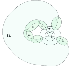
   Figure 9.1. Splash domain $\Omega_{s}$, and the collection of open set $\{U_{0},U_{1},U_{2},...,U_{K}\}$ covering $\Gamma$.

3. For each $l\in\{1,...,K\}$, there exists an $H^{3}$-class diffeomorphism $\theta_{l}$ satisfying

   $$\theta_{l}:B:=B(0,1)\rightarrow U_{l}$$

   $$U_{l}\cap\Omega_{s}=\theta_{l}(B^{+})\ \text{ and }\ \overline{U_{l}}\cap\Gamma_{s}=\theta_{l}(B^{0})\,,$$

   where

   $$B^{+} =\{(x_{1},x_{2},x_{3})\in B:x_{3}>0\}\,,$$

   $$B^{0} =\{(x_{1},x_{2},x_{3})\in\overline{B}:x_{3}=0\}\,.$$

4. For $L>K$, let $\{U_{l}\}_{l=K+1}^{L}$ denote a family of open sets contained in $\Omega_{s}$ such that $\{U_{l}\}_{l=0}^{L}$ is an open cover of $\Omega_{s}$, and for $l\in\{K+1,...,L\}$, $\theta_{l}:B\to U_{l}$ is an $H^{3}$ diffeormorphism.

5. To the open set $U_{0}$ we associate two $H^{3}$-class diffeomorphisms $\theta_{+}$ and $\theta_{-}$ of $B$ onto $U_{0}$ with the following properties:

   $$\theta_{+}(B^{+}) =U_{0}^{+}\,,\qquad\qquad \theta_{-}(B^{+})=U_{0}^{-}\,,$$

   $$\theta_{+}(B^{0}) =\overline{U_{0}^{+}}\cap\Gamma_{s}\,, \theta_{-}(B^{0})=\overline{U_{0}^{-}}\cap\Gamma_{s}\,,$$

   such that

   $$\{x_{0}\}=\theta_{+}(B^{0})\cap\theta_{-}(B^{0})\,,$$

   and

   $$\theta_{+}(0)=\theta_{-}(0)=x_{0}\,.$$

   We further assume that

   $$\overline{\theta_{\pm}(B^{+}\cap B(0,1/2))}\cap\overline{\theta_{l}(B^{+})}=\emptyset\text{ for }l=1,...,K\,,$$

   and

   $$\overline{\theta_{\pm}(B^{+}\cap B(0,1/2))}\cap\overline{\theta_{l}(B)}=\emptyset\text{ for }l=K+1,...,L\,.$$

Definition 9.1 (Splash domain $\Omega_{s}$).

We say that $\Omega_{s}$ is a splash domain, if it is defined by a collection of open covers $\{U_{l}\}_{l=0}^{L}$ and associated maps $\{\theta_{\pm},\theta_{1},\theta_{2},...,\theta_{L}\}$ satisfying the properties (1)–(5) above. Because each of the maps is an $H^{3}$ diffeomorphism, we say that the splash domain $\Omega_{s}$ defines a self-intersecting generalized $\bf H^{3}$-domain.

9.2. An approximating sequence of non self-intersecting domains converging to the splash domain

Following [16], we can then define standard (non self-intersecting) domains $\Omega^{\epsilon}$ (for $\epsilon>0$ small enough) by just modifying $\theta_{\pm}$, and leaving the other charts unchanged. As shown in Figure 9.2, our non self-intersecting domain $\Omega^{\epsilon}$ will be defined by associated maps $\{\theta\epsilon_{\pm},\theta_{1},\theta_{2},...,\theta_{L}\}$ such that

$$\|\theta^{\epsilon}_{\pm}-\theta_{\pm}\|_{H^{3}(B^{+})}\leq C\epsilon\,,$$ (9.1)

and such that

$$0<d(\theta^{\epsilon}_{+}(B^{+}),\theta^{\epsilon}_{-}(B^{+}))\leq\epsilon\,.$$ (9.2)

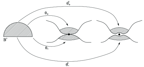
Figure 9.2. The black dot denotes the point $x_{0}$ where the boundary self-intersects (middle). For $\epsilon>0$, the approximate domain $\Omega^{\epsilon}$ does not intersect itself (right).

In summary, we have approximated the self-intersecting splash domain $\Omega_{s}$ with a sequence of $H^{3}$-class domains $\Omega^{\epsilon}$ converging toward $\Omega$, such that for each $\epsilon>0$, $\partial\Omega^{\epsilon}$ does not self-intersect. As such, each one of these domains $\Omega^{\epsilon}$, $\epsilon>0$, will thus be amenable to our local-in-time well-posedness theory for free-boundary incompressible Navier-Stokes equations.

10. Existence of a splash in finite time in a domain arbitrarily close to a given splash domain

We next define an initial velocity field of the same type as in Section 6.1. Due to (9.1), the estimates of Section 7 remain unchanged. Similarly, the main proof of Section 8 works in a similar manner due to (9.2), leading to the necessity of self-intersection at a time $T^{\epsilon}\in(0,10\epsilon)$. Note that since the tangent plane at the intended splash singularity $x_{0}$ is the horizontal plane $\{x_{3}=0\}$, $\partial[\theta_{-}(B^{+})]$ is very close to $\{x_{3}=0\}$ in a small ball $B(x_{0},\sqrt{\epsilon})$ for $\epsilon$ taken sufficiently small; thus, we are using the fact that the almost flat portion of $\theta_{-}(B^{+})$ is very close to $\{x_{3}=0\}$ and contains a region of diameter at least $\sqrt{\epsilon}$.

Furthermore,

$$\|\eta^{\epsilon}(\theta^{\epsilon}_{\pm},T^{\epsilon})-\theta_{\pm}\|_{3} \leq\|\eta^{\epsilon}(\theta^{\epsilon}_{\pm},T^{\epsilon})-\theta^{\epsilon}_{\pm}\|_{3}+\|\theta^{\epsilon}_{\pm}-\theta_{\pm}\|_{3}$$

$$\leq\|\int_{0}^{T^{\epsilon}}v^{\epsilon}(\theta^{\epsilon}_{\pm},t)\ dt\|_{3}+C\epsilon\,,$$ (10.1)

where we used the estimate (9.1) in the above inequality (10.1); hence, from our estimates in Section 7,

$$\|\eta^{\epsilon}(\theta^{\epsilon}_{\pm},T^{\epsilon})-\theta_{\pm}\|_{3}\leq C\mathcal{P}(M_{0})\sqrt{T^{\epsilon}}+C\epsilon\leq C\mathcal{P}(M_{0})\sqrt{\epsilon}\,.$$ (10.2)

This, therefore, shows that the splash-free surface $\eta^{\epsilon}(\Omega^{\epsilon},T^{\epsilon})$ is at a distance less than $C\mathcal{P}(M_{0})\sqrt{\epsilon}$ from $\Omega_{s}$ in $H^{3}$. We have then established the following:

Theorem 10.1.

For any given splash domain $\Omega_{s}$ of class $H^{3}$, there exists a splash domain $\tilde{\Omega}_{s}$ arbitrarily close in $H^{3}$ to $\Omega_{s}$, and smooth initial data consisting of a non self-intersecting domain $\Omega^{\epsilon}$ of class $H^{3}$ and a divergence-free velocity field $u_{0}^{\epsilon}\in H^{3}(\Omega^{\epsilon})$ satisfying $[\operatorname{Def}u_{0}^{\epsilon}\cdot N_{\epsilon}]\times N_{\epsilon}=0$ on $\partial\Omega^{\epsilon}$, such that the flow map $\eta(x,t)$ solving the Navier-Stokes equations (4.1) satisfies $\eta(\partial\Omega^{\epsilon},T^{*})=\tilde{\Omega}_{s}$. That is, in finite time $T^{*}>0$, a splash singularity occurs which is very close to a prescribed self-intersecting geometry.

References

- [1] H. Abels, The initial-value problem for the Navier-Stokes equations with a free surface in -Sobolev spaces, Adv. Differential Equations, 10, (2005), 45–64.
- [2] C. Amrouche and V. Girault, The existence and regularity of the solution of Stokes problem in arbitrary dimension, Proc. Japan Acad., 67, Ser. A, (1991), 171–175.
- [3] C. Amrouche and N.E.H. Seloula, On the Stokes equations with the Navier-type boundary conditions, Differ. Equ. Appl., 3 (2011), 581–607
- [4] H. Bae, Solvability of the free boundary value problem of the Navier-Stokes equations, Discrete Contin. Dyn. Syst., 29, (2011), 769–801.
- [5] J. Beale. The initial value problem for the Navier-Stokes equations with a free surface, Comm. Pure Appl. Math. 34 (1981), no. 3, 359–392.
- [6] J.T. Beale, Large-time regularity of viscous surface waves, Arch. Rational Mech. Anal., 84 (1983/84), 307–352.
- [7] A. Castro, D. Córdoba, C. Fefferman, F. Gancedo, and M. Gómez-Serrano, Finite time singularities for water waves with surface tension, Journal of Mathematical Physics, 53, (2012), 115622–115622.
- [8] A. Castro, D. Córdoba, C. Fefferman, F. Gancedo, and M. Gómez-Serrano, Finite time singularities for the free boundary incompressible Euler equations, Ann. of Math., 178, (2013), 1061–1134.
- [9] A. Castro, D. Córdoba, C. Fefferman, F. Gancedo, and M. Gómez-Serrano, Splash singularities for the free boundary Navier-Stokes equations, (2015), arXiv:1504.02775.
- [10] D. Córdoba, A. Enciso, and N. Grubic, Splash and almost-splash stationary solutions to the Euler equations, (2014), Arxiv preprint arXiv:1412.7382.
- [11] C.H.A. Cheng and S. Shkoller, The interaction of the 3D Navier-Stokes equations with a moving nonlinear Koiter elastic shell, SIAM J. Math. Anal., 42, (2010), 1094–1155.
- [12] D. Coutand, S. Shkoller, Unique solvability of the free-boundary Navier-Stokes equations with surface tension, (2002), arXiv:math/0212116.
- [13] D. Coutand, S. Shkoller, On the motion of an elastic solid inside of an incompressible viscous fluid, Arch. Rational Mech. Anal., 176, (2005), 25–102.
- [14] D. Coutand, S. Shkoller, The interaction between quasilinear elastodynamics and the Navier-Stokes equations, Arch. Rational Mech. Anal., 179, (2006), 303–352.
- [15] D. Coutand and S. Shkoller, Well-posedness of the free-surface incompressible Euler equations with or without surface tension, J. Amer. Math. Soc., 20, (2007), 829–930.
- [16] D. Coutand and S. Shkoller, On the Finite-Time Splash and Splat Singularities for the 3-D Free-Surface Euler Equations, Comm. Math. Phys., 325, (2014), 143–183.
- [17] D. Coutand and S. Shkoller, On the impossibility of finite-time splash singularities for vortex sheets, (2014), arXiv:1407.1479.
- [18] T. Elgindi and D. Lee, Uniform regularity for free-boundary Navier-Stokes equations with surface tension, (2014), arXiv:1403.0980.
- [19] C. Fefferman, A.D. Ionescu, and V. Lie, On the absence of “splash” singularities in the case of two-fluid interfaces, Preprint, (2013), arXiv:1312.2917.
- [20] Y. Hataya, Decaying solution of a Navier-Stokes flow without surface tension, J. Math. Kyoto Univ., 49 (2009), 691–717.
- [21] Y. Guo and I. Tice, Almost exponential decay of periodic viscous surface waves without surface tension, Arch. Ration. Mech. Anal., 207, (2013), 459–531.
- [22] Y. Guo and I. Tice, Decay of viscous surface waves without surface tension in horizontally infinite domains, Anal. PDE 6, (2013), 1429–1533.
- [23] Y. Guo and I. Tice, Local well-posedness of the viscous surface wave problem without surface tension, Anal. PDE, 6, (2013), 287–369.
- [24] N. Masmoudi and F. Rousset, Uniform regularity and vanishing viscosity limit for the free surface Navier-Stokes equations, (2012), arXiv:1202.0657.
- [25] T. Nishida, Y. Teramoto, H. Yoshihara. Global in time behavior of viscous surface waves: horizontally periodic motion. J. Math. Kyoto Univ. 44 (2004), no. 2, 271–323.
- [26] M. Padula and V.A. Solonnikov, On Rayleigh-Taylor stability, Navier-Stokes equations and related nonlinear problems (Ferrara, 1999), Ann. Univ. Ferrara Sez. VII (N.S.), 46, (2000), 307–336.
- [27] V. A. Solonnikov, Solvability of the problem of the motion of a viscous incompressible fluid that is bounded by a free surface, Izv. Akad. Nauk SSSR Ser. Mat., 41 (1977), 1388–1424.
- [28] V.A. Solonnikov, On an initial boundary value problem for the Stokes systems arising in the study of a problem with a free boundary, Proc. Steklov Inst. Math., 3 (1991), 191–239.
- [29] V.A. Solonnikov, Solvability of the problem of evolution of a viscous incompressible fluid bounded by a free surface on a finite time interval, St. Petersburg Math. J., 3 (1992), 189–220.
- [30] V.A. Solonnikov and V.E. Scadilov, On a boundary value problem for a stationary system of Navier-Stokes equations , Proc. Steklov Inst. Math., 125, (1973), 186–199.
- [31] A. Tani, N. Tanaka, Large-time existence of surface waves in incompressible viscous fluids with or without surface tension, Arch. Rational Mech. Anal., 130 (1995), no. 4, 303–314.
- [32] Y. Wang and Z. Xin, Vanishing viscosity and surface tension limits of incompressible viscous surface waves, (2015), arXiv:1504.00152.