Superfluid to normal fluid phase transition in the Bose gas trapped in two dimensional optical lattices at finite temperature

Abstract

We develop the Hartree-Fock-Bogoliubov theory at finite temperature for Bose gas trapped in the two dimensional optical lattices. The on-site energy is considered low enough that the gas presents superfluid properties. We obtain the condensate density as function of the temperature neglecting the anomalous density in the thermodynamics equations. The condensate fraction provide two critical temperature. Below the temperature $T_{C1}$ there is one condensate fraction. Above two possible fractions merger up to the critical temperature $T_{C2}$. Then the gas provides an first order transition at temperature above $T_{C2}$ where the condensate fraction is null. We resume by a finite-temperature phase diagram where can be identify three domains: the normal fluid, the superfluid and the superfluid with two possible condensate fractions.

I Introduction

The Bose-Einstein condensate trapped in the periodic potential provided a peculiar phenomenum in which there exist the quantum phase transition in the ultra-cold atoms similar to the phase transition seen in crystals mor06 ; blo08 . In this transition, the variation of external parameter related to the trap potential modifies the non-local superfluid properties into the local properties of the Mott insulator phase.

At low temperatures, the superfluid-to-Mott-insulator (SF-MI) quantum phase transition was proposed in 1998 by Jaksch et al. jak98 for ultra-cold gases. They considered a Bose-Hubbard model to describe the Bose gas on the optical lattices, and they showed the quantum phase transition by changing the on-site energy, the hopping matrix element or the chemical potential. Four years later, Greiner et al. gre02 detected the SF-MI phase transition by imaging atoms released from optical lattices with different periodic potentials. Above a critical on-site energy, the atomic distribution presents the correlation function concerned to the Mott-insulator. In this phase, the position of atoms gem09 become a tool to probe and measure thermodynamic properties such as pressure, temperature, and transport properties hun10 .

Another way to observe the SF-MI phase transition is analysing the collective excitations in the gas trapped in optical lattices. The low-lying excitation energy of the gas is achieved in 1D via lattice modulation sto04 or by Bragg spectroscopy cle09 . In the superfluid (SF) phase, the energy spectrum presents a gapless behaviour which can be explained within a Bogoliubov theory oos01 , or in terms of path integral formalism kle12 or by Green’s function formalism zal12 .

In Mott insulator (MI) phase, the gapped excitation mode is found by the mean-field theory oos01 using the particle-hole excitations frame of the superfluity modes. The mean-field theory in oos01 neglected the quantum fluctuations, then the description of the system near to SF-MI phase transition is unavailable and, therefore, not confirmed the gapped mode bis11 . The SF-MI transition is analysed in terms of a strong-coupling perturbation theory which treats the kinetic energy as a mean-field and deals exactly the on-site repulsion fis89 ; jak98 . This approximation gave a estimative for the SF-MI transition limits.

The thermal gapless properties of ultra-cold bosons in optical lattices were discussed by Gerbier in the ref. ger07 . However, his analysis were done considering only the Mott insulator phase. At superfluid phase, a finite-temperature study of ultra-cold bosons in 2D optical lattices were done in mah12 by quantum Monte-Carlo simulation taking account the effects of harmonic confinement. In this reference, they observed the spatial inhomogeneity allows the coexistence of three phases: the usual ground state superfluid, the Mott insulator phase and the normal fluid phase. Their simulations can be compared with the phase diagram provided by the experimental results jim10 .

The phase diagram is describe as a function of the temperature and the interaction strength whose definition is the ratio between the on-site interaction strength and the hopping matrix element. The phase diagram for the homogeneous 3D system at unity filling is plotted using the quantum Monte Carlo simulation in the reference cap07 and shown experimentally in tro10 . At zero temperature, the system undergoes a SF-MI quantum phase transition at the critical interaction strength. At temperatures different from zero and near to the critical interaction strength, they observed a suppression of the critical temperature where the condensate fraction is null and all particles are in the thermal cloud.

In this work, we investigate the thermal behaviour of the ultra-cold Bose gas in 2D optical lattices on the superfluid phase and far from the SF-MI phase transition by a finite-temperature mean-field theory. This theory is known as Hartree-Fock-Bogoliubov (HFB) theory and departing from the Bose-Hubbard model. Although the HFB theory provide a gapped spectrum even far from the quantum phase transition, we avoid this problem by the Popov approximation where the anomalous densities are neglected ad hoc. Hence the spectrum is gapless and, as theoretically shown in oos01 and experimentally observed in bis11 , the condensate fraction has the superfluid properties and depends on the temperature and the interaction strength. Then, in HFB theory, the superfluid phase has, as order parameter, the fraction of condensate. We determine the order parameter as function of the temperature at a regime below to the quantum phase transition.

In sec. II we obtain the HFB theory considering the superfluid state as a vacuum of the quasi-particles at finite temperature, we determine the limits to the Bogoliubov theory and we implement the Popov approximation to derive the condensate fraction. The numerical solution for the condensate fraction in the Popov approximation is evaluated in the sec. III. Finally, in sec. IV, we discuss the properties of the system near the thermal phase transition according to the solution of the mean-field theory.

II Hartree-Fock-Bogoliubov approximation at finite temperature

The dynamics of the 2D ultra-cold boson gas in the optical lattices can be done by the second quantized Hamiltonian,

$$H = \int\psi^{\dagger}({\bf x})\left(-\frac{\hbar^{2}\nabla^{2}}{2m}+V_{0}({\bf x})+V_{T}({\bf x})\right)\psi({\bf x})d^{3}{\bf x}+$$

$$+ \frac{1}{2}\frac{4\pi a_{s}\hbar^{2}}{m}\int\psi^{\dagger}({\bf x})\psi^{\dagger}({\bf x})\psi({\bf x})\psi({\bf x})d^{3}{\bf x}$$

where $\psi({\bf x})$ is the boson field operator corresponding to the atom with the mass equal to $m$, $V_{T}({\bf x})=\frac{m}{2}\sum_{j=1}^{3}\omega_{j}^{2}x_{j}^{2}$ is the magneto-optical trap and $V_{0}({\bf x})=V_{0}(\sin^{2}(\pi x/a)+\sin^{2}(\pi y/a))$ is the external periodic potential formed by the intersecting laser beams with $V_{0}$ being the trap depth proportional to the laser intensity, $a$ being the less distance between two sites. In this Hamiltonian, the inter-atomic interaction corresponds to the low-energy collision characterized by the $s$-wave scattering length, $a_{s}$.

We expand the field operators in Wannier functions whose asymptotic behaviour is adjusted by the Gaussian function, $w({\bf x})=e^{-(x^{2}+y^{2})/2\sigma^{2}}/(\pi^{1/2}\sigma)^{1/2}$ with $\sigma=\hbar/(m^{2}V_{0}E_{R})^{1/4}$ and $E_{R}=\hbar^{2}\pi^{2}/(2ma^{2})$ is the recoil energy. Considering only the lowest vibrational state in each site, the field operator can be written as, $\psi({\bf x})=\sum_{i}w({\bf x}-{\bf x}_{i})\alpha_{i}$, where ${\bf x}_{i}$ is the position of the site labelled by $i$ in the 2D lattices with $N_{s}$ sites. Thus, in terms of the Wannier operators $\alpha_{i}$, the Hamiltonian become a Bose-Hubbard (B-H) Hamiltonian,

$$H=-t\sum_{\langle i,j\rangle}\alpha_{i}^{\dagger}\alpha_{j}+\frac{1}{2}U\sum_{i}\alpha_{i}^{\dagger}\alpha_{i}^{\dagger}\alpha_{i}\alpha_{i},$$ (2)

where $t=-\int w^{*}({\bf x}-{\bf x}_{i})\left(-\frac{\hbar^{2}\nabla^{2}}{2m}+V_{0}({\bf x})\right)w({\bf x}-{\bf x}_{j})d^{3}{\bf x}$ is the hopping parameter and $U=\frac{4\pi a_{s}\hbar^{2}}{m}\int|w({\bf x})|^{4}d^{d}{\bf x}$ is the on-site interaction strength. The hopping parameter is the same for any site due to neglect the magneto-optical trap effects, $V_{T}({\bf x})=0$.

In order to identify the condensate state, we expand the Wannier operators in the 2D quasi-momentum space, $\alpha_{i}=\frac{1}{\sqrt{N_{s}}}\sum_{\bf k}a_{\bf k}e^{-\imath(k_{x}x_{i}+k_{y}y_{i})}$, where the component of quasi-momentum, ${\bf k}$, assume discrete values give by $k_{j}=2\pi\eta/(M_{j}a)$ with $\eta=0,\pm 1,\pm 2,\cdots,\pm(M_{j}-1)/2$ and $M_{j}$ is the even number corresponding to the number of site in the $j$-direction.

The condensate state is a coherent state of $N_{0}$ single particles with quasi-momentum equal to zero. We represent this state in the B-H Hamiltonian by shifting the zero quasi-momentum operator, $a_{\bf k}=b_{\bf k}+\sqrt{N_{0}}\delta_{\bf 0,k}$. Then we have the shifted B-H Hamiltonian as,

$$H = (-\bar{\epsilon}_{0}-\mu)N_{0}+\frac{g}{2}N_{0}^{2}+\sqrt{N_{0}}(-\bar{\epsilon}_{0}-\mu+gN_{0})(b_{0}+b^{\dagger}_{0})+$$

$$+ \sum_{\bf k}\left[(-\bar{\epsilon}_{\bf k}-\mu+2gN_{0})b^{\dagger}_{\bf k}b_{\bf k}+\frac{g}{2}N_{0}(b_{\bf k}b_{-\bf k}+b^{\dagger}_{\bf k}b^{\dagger}_{-\bf k})\right]+$$

$$+ z_{0}g\sum_{\bf kq}(b^{\dagger}_{\bf k+q}b^{\dagger}_{\bf k}b_{\bf q}+b^{\dagger}_{\bf k-q}b_{\bf k}b_{\bf q})+\frac{g}{2}\sum_{\bf kk^{\prime}q}b^{\dagger}_{\bf k+q}b^{\dagger}_{\bf k^{\prime}-q}b_{\bf k}b_{\bf k^{\prime}},$$

where $\bar{\epsilon}_{\bf k}=2t(\cos(k_{x}a)+\cos(k_{y}a))$ is the energy of the free quasi-particles, $g=U/N_{s}$ is the interaction parameter and $\mu$ is the chemical potential in which ensures a well-defined particle number even for the particle reservoir contact.

For the purpose of decoupling normal modes, we introduce the Bogoliubov transformation, $b^{\dagger}_{\bf k}=u_{\bf k}c^{\dagger}_{\bf k}+v_{\bf k}c_{\bf-k}$ where $u_{\bf k}$ and $v_{\bf k}$ are the real Bogoliubov coefficients and obey $u^{2}_{\bf k}-v^{2}_{\bf k}=1$ to keep the commutation relations. The Bogoliubov coefficients are adjusted for becoming the B-H Hamiltonian in diagonal form, $H=E_{0}+\sum_{\bf k}E_{k}c^{\dagger}_{\bf k}c_{\bf k}$, where $E_{0}$ is the ground state energy and $E_{k}$ is the excitation energy.

Assuming the time invariance of the Bogoliubov coefficients, we derive the excitation energy as, $E_{k}=\sqrt{h^{2}_{k}-\Delta^{2}}$, and the Bogoliubov coefficients are, $v^{2}_{k}=\frac{1}{2}\left(\frac{h_{k}}{E_{k}}-1\right)$ and $u_{k}v_{k}=-\frac{1}{2}\frac{\Delta}{E_{k}}$, where the parameters $h_{k}=\bar{\epsilon}_{0}-\bar{\epsilon}_{k}+g(N_{0}-\sum_{k}\kappa_{k})$ and $\Delta=g(N_{0}+\sum_{k}\kappa_{k})$ depend on the variational parameters, $\rho_{k}=\nu(k,T)+(1+2\nu(k,T))v^{2}_{k}$ and $\kappa_{k}=(1+2\nu(k,T))u_{k}v_{k}$. These parameters are thermal averages of shifted operator and depend on the temperature bla87 . The function $\nu(k,T)=(e^{E_{k}/k_{B}T}-1)^{-1}$ is the Bose-Einstein distribution of a quantum particle with energy equal to $E_{k}$.

Finally, we can obtain the chemical potential in terms of the number of the condensed particles, $N_{0}$, the depleted particles, $\sum_{k}\rho_{k}$ and the paring, $\sum_{k}\kappa_{k}$. The chemical potential is written as $\mu=-\bar{\epsilon}_{0}+g[N_{0}+\sum_{k}(2\rho_{k}+\kappa_{k})]$.

II.1 Particle number

To evaluate the condensate fraction $n_{0}=N_{0}/N_{s}$ as an explicit function of the dimensionless interaction strength, $U/t$, and the temperature, $T$, we introduce the total density in each site by, $n=\sum_{\bf k}\langle a^{\dagger}_{\bf k}a_{\bf k}\rangle/N_{s}$. In terms of the Bogoliubov parameters, the depletion density is given by, $n-n_{0}=\sum_{\bf k}\rho_{\bf k}/N_{s}$. Hence, we have the condensate density in each site as,

$$n_{0}=n-\frac{1}{N_{s}}\sum_{\bf k}\frac{1}{2}\left(\coth\left(\frac{E_{k}}{2k_{B}T}\right)\frac{h_{\bf k}}{E_{k}}-1\right),$$ (4)

where, $h_{\bf k}=\zeta_{k}+U(n_{0}-m_{0})$, $\Delta=U(n_{0}+m_{0})$ and $\zeta_{k}=4t[\sin^{2}(k_{x}a/2)+\sin^{2}(k_{y}a/2)]$.

The anomalous density in each site, $m_{0}=(\sum_{k}\kappa_{k})/N_{s}$, can be an explicit form that depend on the condensate density, $m_{0}=-n_{0}(\sum_{k}\coth(E_{k}/2k_{B}T)/E_{k})/(2/U+\sum_{k}\coth(E_{k}/2k_{B}T)/E_{k})$. If the anomalous density is different from zero, we have a gap in the excitation spectrum given by, $\lim_{{k}\to 0}E_{k}=2U(-n_{0}m_{0})^{1/2}$.

II.2 Popov approximation

In the HFB theory, the excitation spectrum presents a gap for long-wavelength excitations and, therefore, not satisfies the Hugenholtz-Pines theorem gri96 ; hoh65 . Indeed, the gap in the spectrum for long-wavelength can not explain the superfluid properties, as the absence of viscosity lan80 ; gri93 , widely identified due to the phonon behaviour of the excitation spectrum in ultra-cold alkaline atoms ket00 .

At very low temperatures and in the very weakly interaction regime, the condensate fraction is high enough to neglect the depletion, $n_{0}\approx n$, and the anomalous density $m_{0}=0$. By this approximation, known as Bogoliubov approximation, the excitation energy, $E_{k}=\sqrt{\zeta_{k}(\zeta_{k}+2nU)}$, is gapless for the long-wavelength limit and the condensate density depends only on the total density, $n$.

Otherwise, we can neglect ad hoc only the anomalous density, $m_{0}=0$. The so-called Popov approximation provides a non-linear integral equation to the condensate density given by,

$$n_{0}=n-\frac{1}{2N_{s}}\sum_{\bf k}\frac{\coth\left(E_{k}/2k_{B}T\right)(\zeta_{k}+n_{0}U)-E_{k}}{E_{k}},$$ (5)

with a gapless spectrum equal to $E_{k}=\sqrt{\zeta_{k}(\zeta_{k}+2n_{0}U)}$.

III Numerical results

We obtain the condensate fraction, $n_{0}/n$, as function of the temperature and the dimensionless interaction strength parameter, $U/t$, solving numerically the non-linear equation (5) derived by the Popov approximation.

At zero temperature, we plot in fig. 1 the condensate fraction as function of the interaction strength for four sizes of the 2D squared lattice. When we increase the size of the lattice, the condensate fraction converge to an asymptotic curve regarded to the thermodynamic limit. Then, as the difference between the curves provide for lattice with $101\times 101$ and $501\times 501$ is small and for the sake of the computation time, we assume the size of lattice equal to $101\times 101$ can be considered in the thermodynamic limit.

In the ref. oos01 , they analysed the limits for the strongly interacting regime, $U/t\to\infty$, at zero temperature and they concluded that the quantum phase transition could not be identified in the Bogoliubov approximation. However the arguments used to justify the absence of phase transition are based on the Popov approximation indeed. We observe the same result in the fig. 1 for any size of lattice using the Popov approximation. Differently from them, it is not clear for us the rule of the Bogoliubov approximation in this lack of the quantum phase transition.

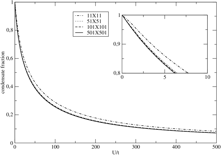
Figure 1: The condensate fraction $n_{0}/n$ in two-dimensional lattice as function of the dimensionless interaction strength parameter $U/t$ at zero temperature. The graph exhibits the approach to the thermodynamic limit in which the ration $N/N_{s}=n$ remains constant. This approach is realized when the size of the lattice exceeds $10^{4}$ sites.

In order to obtain the temperature-dependent condensate fraction, we introduce the function,

$$f(x)=1-x-\frac{1}{nN_{s}}\sum_{\bf k}\frac{1}{2}\left(\coth\left(\frac{\sqrt{\epsilon_{\bf k}(\epsilon_{\bf k}+2nUx)}}{2k_{b}T}\right)\frac{\epsilon_{\bf k}+nUx}{\sqrt{\epsilon_{\bf k}(\epsilon_{\bf k}+2nUx)}}-1\right),$$ (6)

where the variable $x$ running from $0$ to $1$. The function $f(x)$ is determined by the temperature $T$ and the interaction strength parameter $U/t$ and its roots are the condensate fractions at this temperature and for this interaction strength. In fig. 2 we plot this function for $U/t=10.0$ and at different temperatures. The plot exhibits three different types of the solution for equation (5). There is one solution for $0\leq T\leq T_{C1}$, where $T_{C1}$ is the temperature in which the function $f(x)$ presents a root at $x=0$. When we increase the temperature, we find two solution which merger at $T=T_{C2}$. At temperatures larger than $T_{C2}$, there is no solution and, therefore, there is no condensate fraction in the lattice.

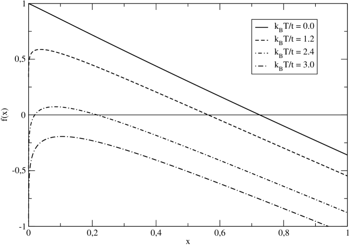
Figure 2: The function $f(x)$ (eq. 6) is plotted for different values of the temperatures and for $n=1.0$, $U/t=10.0$ and $N_{S}=101\times 101$. This graph illustrates the numerical method used to find the roots of $f(x)$.

In the fig. 3 we plot the condensate fraction as function of the temperature for different values of the interaction strength. In the non-interacting case $U/t=0.0$, the fraction decrease when the temperature increase and reach a null fraction, i. e., the condensate disappear at the temperature $T_{C1}=1.6954$ (in units of $k_{B}/t$). Above this critical temperature the gas is entirely a thermal Bose fluid and the quasi-particles have free energy dispersion in the limit of the large wavelength.

For the interacting case $U/t\neq 0.0$, there are only one condensate fraction in the interval of the temperature $0\leq T\leq T_{C1}$. In this condition, the values of the fraction decrease as temperature increase. For the temperature in the range of $T_{C1}<T<T_{C2}$, there are two possible condensate fractions. Differently from the largest fraction which decreases as the temperature increases, the smallest fraction increases up to merger the highest fraction at the second critical temperature $T_{C2}$. At temperature above $T_{C2}$, there is no solution for $f(x)$ and, therefore, there is no condensate in the lattice.

The fig. 3 shows that exist an interval of the temperature in which the strongly interacting Bose gas ($U/t=10.0$) presents the condensate fraction larger than the condensate fraction of the weakly interacting Bose gas ($U/t=0.1$). This unusual behaviour is contrary to what intuition or common sense would indicate.

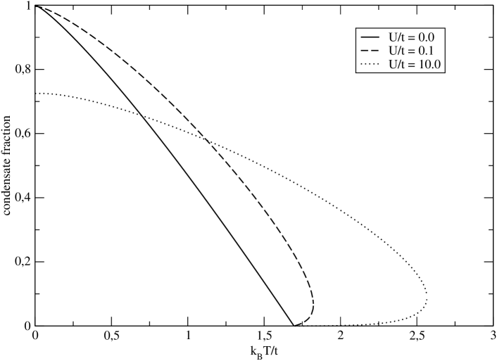
Figure 3: The condensate fraction $n_{0}/n$ as a function of the temperature $T$ for different values of the interaction strength parameter $U/t$ in the same conditions of 2. Three interacting regimes are deal in the figures. The non-interacting gas is describe by the solid curve, the weakly interacting gas is shown in the traced line, and the strongly interacting gas is represented by the dotted curve.

The phase diagram shown in the fig. 4 has three regions correspond to the possible values of the condensate fraction. The region SF where there is one condensate fraction, CSF in which coexists two possible condensate density and the region NF composed by the thermal free quasi-particles. As we increase the interaction strength parameter, the CSF region increases monotonically.

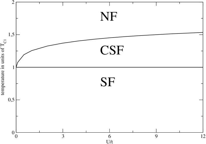
Figure 4: Finite-temperature phase diagram as a function of dimensionless parameter $U/t$ and temperature $T$ of the Bose gas trapped in two dimensional lattice with size of $N_{S}=101\times 101$ and density equal to $n=1.0$.

Finally, in the fig. 5 we present the condensate fraction $n_{0}/n$ in two dimensional lattice as a function of the interaction strength parameter at several temperatures. At temperature below the critical temperature $T_{C1}$, the condensate fraction increase when the interaction parameter increase. This growth is provided by the positive contribution of the interaction. The repulsive interaction promotes the non-localization of the atoms in the lattice. Although the effect of the interaction, the entropy plays the leading role for large values of the interaction parameter. Then, the maximum value of the condensate fraction is reached around $U/t\approx 0.5$, and the fraction decreases monotonically up to zero in the limit of strongly interaction. At temperatures higher than the critical temperature $T_{C2}$, the curves present a minimum value to the interaction parameter in which the two possible solution of the condensate fraction rise. As the case of low-temperature, there is a balance between the interaction and the entropy. For interaction parameter close to the critical parameter, the role of the interaction is more determinant than the entropy. However the entropy dominates for the limit of the strongly interacting regime.

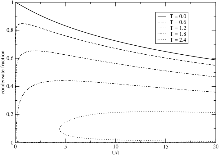
Figure 5: The condensate fraction $n_{0}/n$ as a function of the dimensionless parameter $U/t$ at different temperatures (in units of $t/k_{B}$) with $n=1.0$ and $N_{S}=101\times 101$. At temperatures below $T_{C1}$, the curves are positive functions with only one maximum point. At temperature above, the curves present a minimum critical value for the dimensionless parameter $U/t$ where below there is no condensate at this temperature. For above the critical dimensionless parameter, the condensate can coexist in two possible condensate fraction.

IV Summary

We develop the Hartree-Fock-Bogoliubov theory at finite temperature for Bose gas trapped in the two dimensional optical lattices. This mean-field theory presents anomalous pairing density in which provides a gap in the energy spectra for large wavelength excitation.

To obtain a gapless excitation energy, we consider the Popov approximation where the anomalous density is neglected ad hoc. In the Popov approximation, we derive a non-linear equation whose solutions give us the condensate fraction in the system. Considering the size of the lattices large enough to be in the thermodynamic limit, we obtain curve of condensate fraction as function of the temperature. These curves present two critical temperature, one of them $T_{C1}$ define an interval where we have a single order parameter. Above this temperature, there are two condensate fraction that merger at the critical temperature $T_{C2}$. Then the gas provides an first order transition when temperature pass over $T_{C2}$ and, in this condition, the condensate fraction is null. We identify an interval of the temperature in which the strongly interacting gas has the condensate fraction large than the weakly interacting gas. This unusual effect is due to the balance between the role of the entropy and the interaction.

A phase diagram as a function of interaction strength $U/t$ and temperature $T$ is done calling attention to the regions where occur the normal fluid phase, the superfluid phase and the superfluid phase in which coexist two different condensate fractions. There is a decay behaviour when the interaction strength approach to the zero as observed by cap07 using the quantum Monte Carlo simulation for 3D lattice. Then the HFB theory is qualitatively usefull to describe the condensate fraction in the weakly interacting regime. The quatitative comparison between the HFB theory and the Monte-Carlo simulation is out of scope and it will be done in future work. Otherwise, for large interaction strength, the thermal phase transition temperature increase and, therefore, frustrates any possibility to identify the quantum phase transition by the mean-field theory. Indeed, the trial function to develop the HFB theory is not appropriated to describe the strongly correlated lattice.

- (1) O. Morsch and M. Oberthaler, Rev. Mod. Phys. 78, 179 (2006).
- (2) I. Bloch, J. Dalibard, and W. Zwerger, Rev. Mod. Phys. 80, 885 (2008).
- (3) D. Jaksch, C. Bruder, J. I. Cirac, C. W. Gardiner, and P. Zoller, Phys. Rev. Lett. 81, 3108 (1998).
- (4) M. Greiner, O. Mandel, T. Esslinger, T. W. Hansch, and I. Bloch, Nature 415, 39 (2002).
- (5) N. Gemelke, X. Zhang, C. Hung, and C. Chin, Nature 460, 995 (2009).
- (6) C. L. Hung, X. Zhang, N. Gemelke, and C. Chin, Phys. Rev. Lett. 104, 160403 (2010).
- (7) T. Stoferle, H. Moritz, C. Schori, M. Kohl, and T. Esslinger, Phys. Rev. Lett. 92, 130403 (2004).
- (8) D. Clement, N. Fabbri, L. Fallani, C. Fort, and M. Inguscio, Phys. Rev. Lett. 102, 155301 (2009).
- (9) D. van Oosten, P. van der Straten, and H. T. C. Stoof, Phys. Rev. A 63, 03601 (2001).
- (10) H. Kleinert, Z. Narzikulov, and A. Rakhimov, Phys. Rev. A 85, 063602 (2012).
- (11) T. A. Zaleski, Phys. Rev. A 85, 043611 (2012).
- (12) U. Bissbort, Y. Li, S. Gotze, J. Heinze, J. S. Krauser, M. Weinberg, C. Becker, K. Sengstock, and W. Hofstetter, Phys. Rev. Lett. 106, 205303 (2011).
- (13) M. P. A. Fisher, P. B. Weichman, G. Grinstein, and D. S. Fisher, Phys. Rev. B 40, 546 (1989).
- (14) F. Gerbier, Phys. Rev. Lett. 99, 120405 (2007).
- (15) K. W. Mahmud, E. N. Duchon, Y. Kato, N. Kawashima, R. T. Scalettar, and N. Trivedi, Phys. Rev. B 84, 054302 (2011).
- (16) K. Jimenez-Garcia, R. L. Compton, Y.-J. Lin, W. D. Phillips, J. V.Porto, and I. B. Spielman, Phys. Rev. Lett. 105, 110401 (2010).
- (17) B. Capogrosso-Sansone, N. V. Prokof’ev, and B. V. Svistunov, Phys. Rev. B 75, 134302 (2007).
- (18) S. Trotzky, L. Pollet, F. Gerbier, U. Schnorrberger, I. Bloch, N. V. Prokof’ev, B. Svistunov, and M. Troyer, Nature Phys. 6, 998 (2010).
- (19) J. -P. Blaizot and G. Ripka, Quantum Theory of Finite Systems (MIT Press, Cambridge, 1987).
- (20) A. Griffin, Phys. Rev. B 53 9341 (1996).
- (21) P. C. Hohenberg and P. C. Martin, Ann. Phys. (NY) 34 291 (1965).
- (22) A. Griffin Excitations in a Bose-Condensed Liquid (Cambridge: Cambridge University Press, (1993)).
- (23) L. D. Landau and E. M. Lifshitz Statistical Physics, Third Edition, Part 1: Volume 5 (Butterworth-Heinemann, (1980)).
- (24) M. R. Andrews, D. M. Kurn, H. -J. Miesner, D. S. Durfee, C. G. Townsend, S. Inouye and W. Ketterle, Phys. Rev. Lett. 79 553 (1997).