Religion-based Urbanization Process in Italy: Statistical Evidence from Demographic and Economic Data

Abstract

This paper analyzes some economic and demographic features of Italians living in cities containing a Saint name in their appellation (hagiotoponyms). Demographic data come from the surveys done in the 15th (2011) Italian Census, while the economic wealth of such cities is explored through their recent [2007-2011] aggregated tax income (ATI). This cultural problem is treated from various points of view. First, the exact list of hagiotoponyms is obtained through linguistic and religiosity criteria. Next, it is examined how such cities are distributed in the Italian regions. Demographic and economic perspectives are also offered at the Saint level, i.e. calculating the cumulated values of the number of inhabitants and the ATI, ”per Saint”, as well as the corresponding relative values taking into account the Saint popularity. On one hand, frequency-size plots and cumulative distribution function plots, and on the other hand, scatter plots and rank-size plots between the various quantities are shown and discussed in order to find the importance of correlations between the variables. It is concluded that rank-rank correlations point to a strong Saint effect, which explains what actually Saint-based toponyms imply in terms of comparing economic and demographic data.

Keywords: Econophysics, Italy, urbanization process, ranking, number of inhabitants, tax income, correlation, hagiotoponyms.

1 Introduction

The impact of religion on the demographic and economic evolution of the societies has been clearly stated in several studies. In the endless list of such contributions, one should mention the (not recent but very interesting) survey on this topic of Iannaccone (1998), but also Iannaccone (1991), Ellison and Sherkat (1995), Lehrer (1995, 1999), Waters et al. (1995) and, more recently, Caltabiano et al. (2006), Zhang (2008), Yeatman and Trinitapoli (2008), Connor (2011) and Connor and Koenig (2015). The quoted papers deal with the social dimension of the religion for what concerns themes like marriage, education, population flows and socio-cultural economics.
A field of research quite neglected by economists and socio-scientists is that related to the influence of religion on the urbanization process, along with an exploration of its historical grounds economic and demographic characteristics.
It is indeed widely accepted that many cities have developed on various seeds, e.g. water sources, river bridges, ores, …, but many exist due to some ”religious purpose”, in a large sense (see Durkheim, 1968, Eliade, 1978, Dubuisson, 2003, Dennett, 2006, Stark and Bainbridge, 1979). The cult allowed splitting, thus necessarily juxtaposing, the human experience of reality into sacred and profane space and time.
In catholic religion, much religious activity is performed through the cult of Saints, considered as intercessors with ”God”. Their bones and relics could even make ”miracles”. The cult of Saints emerged in the 3rd century and gained momentum from the 4th to the 6th century. It formed from Greek and Roman veneration of divinities, heroes, and rulers. It was established at ”sanctified locations” which in turn could attract pilgrims, ”priests”, and merchants, and thus did grow in population size, and became cities. No need to say that it took many centuries before some strong organization around the cult of some Saint developed. It is well known that rival clergy up to bishops and their cliques have been fighting lengthy battles over who had the right to claim the Saint for their own community and even scorning ”rival Saints”. Whether there were economic conditions in play at those times is not a question raised here, - the answer seeming obvious. One of the causes of the protestant reformed is well known indeed.
In Italy (IT, hereafter), known as a basically catholic country, - being closely related to the siege of the papacy, there has been for a while an important motivation about the cult of Saints, to the point that several cities bear the name of a Saint (Webb, 1996).
This paper explores the main characteristics of the Italian society when isolating citizens living in the ”cities with a Saint name”, i.e. hagiotoponym cities (see Reading, 1996). Specifically, this religion-based relevant cultural aspect of the Italian urbanization process is described under a demographical and economical point of view. In particular, we aim at exploring what Saint-based toponyms imply in terms of the comparison between economic and demographic data.
One may thus first wonder how many of these cities appeared and where they are located. Also, it seems to be important to explore how important are they with respect to the population size.
These questions can be justified as being related to studies on social science and urban planning. Some motivation also arises from touristic, geographical, and cultural points of view.
A third concern, but related to the previous one, is of linguistics origin, i.e. a search for the statistical distribution of names of Saints attached to city names. The reader is addressed to the Dictionary of Farmer and Hugh (1987). A related question concerns the rare Saints, e.g. those occurring only once, so called hapaxes; how many of them? The question ”why are such Saints rare?” is outside the purpose of the present report. Nevertheless, how they geographically distributed is an original question.
A fourth motivation of our investigation, but not the least, is based on economics concern. How does being a hagiotoponym city, behave with respect to others? Moreover, is a specific Saint ”better”, in an economic sense, than another?
Therefore, the first question being tackled in this report is: what city and how many, in IT, have a ”Saint” name in its appellation? The (not so trivial as it could be thought, at first) methodology is explained in Sect. 2. In particular, the data acquisition needs some very careful work as explained in Sect. 2.1. Note that a distinction will be made between male and female Saints. In Sect. 2.2, we define the economic and demographic quantities which have retained our attention.
Moreover, it seems of complementary interest to observe the occurrence of less frequent Saints, e.g. dislegomena Saints. Indeed, one might have asked, at the time of rising of such cities whether some novelty in names (or cult), some rarity or in a contrario some popularity of a Saint, would have been (and is still) beneficial within some ”competition”.
In studies of cities, one often examines the rank-size or size-frequency relationships, in accord to Vining (1977) and Chen (2012). Their analysis will be the main content of the figures displayed here below in Appendix B and commented in Sect. 3. For what concerns the rank-size analysis, a brief comment is needed. Often, Zipf’s law (Zipf, 1949) is able to fit the relationship between the size and the rank of a given variable. Such a regularity has not a strong theoretical ground (see Krugman, 1995), and it is shown not to provide a robust analysis of the connections between demographic and economic data in our specific context. In this respect, it is important to note that Zipf’s law fails in several cases (see e.g. Giesen and Sudekun, 2011; Soo, 2007; Cordoba, 2008; Garmestani et al., 2008; Bosker et al., 2008; Vitanov and Ausloos, 2015). For this major reason, we have considered more general rank-size rules based on the Lavalette’s law (Lavalette, 1966). In doing this, we have found robust best fits results, with high levels of $R^{2}$ and interesting interpretations. More specifically, in order to observe how many Saints (or cities) concern the above questions, plots for the rank-size, size-frequency and cumulative distribution function can be made and are presented in order to find an appropriate empirical law: see Sect. 3.
The $density$ of Saints, with respect to the whole country, and with respect to regions should give some idea on ”$catholicity$” (or some $cult$) ”touristic spreading”, at the time of community creations. Thus, whether there is any geographical distribution, with special Saints in some area, is discussed as well; see Sect. 3.2. Next, since cities have often developed around churches or chapels, the question is raised whether there is any relation between ”cities with Saint names” (hagiotoponyms) and present city population size. Moreover, are the most popular Saints associated with ”large” cities? Is the cumulative distribution of interest? In so doing, one may next wonder about the wealth of such cities. How do they fare nowadays? This is examined through the (modern) aggregated income taxes (ATI) of such cities – which represents the aggregate contribution that the citizens of each city provide to the national Gross Domestic Product (GDP) – in Sect. 3.5. The final answer to these questions is found through rank-rank correlation studies, in Sect. 3.6.
Section 3 contains also a comparison between the overall IT cities situation and the set of hagiotoponyms in the respect of demographic and economic variables. It seems that the hagiotoponym cities build a reality similar to the IT one, when the biggest cities are removed as outliers. We strongly emphasize the condition or constraint.
Note that there is no discussion here below concerning parishes nor churches nor chapels nor folk life events implying Saints. This demands a very complex survey; thus is not studied here. In this respect, an interesting paper is Kim (2007) on pilgrimage and towns in medieval christianity. We recommend its reading both for the outlined ideas but also for the bibliography. Nevertheless, we stress that pilgrimage towns do not necessarily have a Saint for name. Cities we examine here below are in fact very rarely pilgrimage towns, though they have local Saint activities.
Moreover, questions on why religious cities grow or fail, and why several Saints are more popular than others are left for further work; see Stark (1996) for a starting point.
A brief conclusion is found in Sect. 4. Appendix A contains the needed statistical toolkit employed for the analysis of the data, while Appendix B contains the Figures and Tables presented.

Remark. When finishing writing this paper, we became aware of a University of Birmingham 2009 Master of Philosophy thesis, by C.H. Morris (Morris, 2009) who examined quite related topics, i.e. the practice of venerating holy figures and their relics, and events that surround such worship, in Anglo-Saxon and Medieval England. Indeed, more or less quoting Morris’ thesis abstract:

• ”[The cult of Saints] was a cultural phenomenon that engaged all sections of society, and Saints enjoyed high levels of popularity through their cults. Not all instances were the same, and cults differed in size and construction. The distances over which cults could command attention varied, as did the social groupings that they catered for.”

This very interesting work differs from ours, surely about the respectively concerned lands, England $vs.$ Italy, the timing, and scientific approaches, but is highly complementary. We emphasize that we add much to this sort of investigations by considering also economic questions.

2 Construction of the dataset

In IT, there are 8092 cities or, better, municipalities (in Italian: comuni) shared among 20 regions nowadays. Thus, data on population size and on ATI have been collected at the municipality level, before selecting the cities of interest.
Specifically, we want to identify the municipalities which have a toponym related to a Saint, so called $hagiotoponyms$. Sometimes, it is not so easy to understand who is the truly related Saint. For example, Giovanni could be the ”apostle” or the ”baptist”. However, we consider that he is most likely Giovanni the apostle. Indeed, the baptist is now called ”Giovanni Battista” of ”Gianbattista”. A check of the official list of Saints on Farmer (1987), indicates that Giovanni can be associated also to more recent people, but this is irrelevant to a city original appellation. The identification of the true Saint is sometimes not possible. Therefore, we decided neither to pursue nor explore such a task further. The Saint name in our list will point to a unique Saint, who is then considered to be the representative element of the related category of the Saints with the same name. It might be relevant to remove this constraint in more advanced religious studies. We also understand that a Saint having given his/her name to a city is not necessarily a bona fide catholic Saint, but only a ”Saint by tradition” (see Farmer, 1987). We do not consider this ambiguity relevant to our consideration, - on the contrary.

2.1 Data acquisition

The investigated data is of three different natures: population data and economic data, and the city names.

• The source of the population data is the Italian Institute of Statistics (ISTAT). In particular, data on the population are extracted from the elaborations of the 15th Italian Census, performed by ISTAT in 2011.
  The population data taken for the municipalities are: number of inhabitants, males and females, number of families, people living in a family, average number of the components of a family, people living as cohabitant and not as a family. Not all such statistical data can be examined here with respect to our concerns, but we recommend the data sources for subsequent work.

• The economic data, i.e. aggregated tax income (ATI), was obtained from (and by) the Research Center of the Italian Ministry of Economics and Finance (MEF). It covered the 2007-2011 time window. The number of cities in IT, and their regional or provincial membership have changed during this time interval, - in fact going from 8101 to 8092. In order to quantify the cities from some economic point of view, we have averaged the ATI of each city over that time window (denoted as $<ATI>$), taking into account the official merging of specific cities, when necessary.
  A warning is in order: the number of hagiotoponym cities has remained constant in the considered time interval. However, it was found that two hagiotoponym cities changed regions: San Leo and Sant’Agata Feltria moved from Marche to Emilia Romagna in 2009. However, the available official data considers such an administrative change as appearing in 2008. To be scientifically consistent, we agree with the official dataset and consider such municipalities as belonging to Marche in 2007 and Emilia Romagna after 2007.

• The data collection here above mentioned relies on the identification of Italian cities having a toponym recalling a Saint. Such an identification has been a tedious stage. It was implemented in several phases which seemed worthwhile of presentation for justifying the subsequent data. Firstly, a preliminary list of cities has been constructed through the application of four sorting procedures. Secondly, a refinement of the preliminary list has been applied, and some municipalities have been ejected on the basis of our own established criteria. After this second phase, the list of municipalities with ”Saint” appellation has been revised one by one. We make more precise here below the applied procedure.
  The preliminary list moves from the premise that some specific toponym might come out from deformations of the original Saint name. Therefore, the string ”san” -which, at a first look, seems to be rather informative, being actually contained also in the words ”santo”, ”santa”, ”sant”, - would in fact lead to the removal of a number of acceptable municipalities from the full list of cities (like Camposampiero, in Veneto, which derives from San Pietro). Thus, we provide a first sorting procedure by employing the string ”sa” to the entire collection of 8092 elements. The resulting list contains 1321 municipalities. The second sorting procedure has been attained by employing the strings ”San ”, ”Santo ”, ”Santa ”, ”Sant’ ” (note the blank space at the end of the strings) for the list of 1321 municipalities. This second sorting has produced 636 municipalities containing at least one of the strings and the remaining 685 ones without the strings. The third sorting procedure has been implemented on the group of 685 municipalities, in view of further facilitating the identification of the municipalities of interest. The string ”san” (without space after the word) has been employed; whence it is found that 180 municipalities contain ”san” and the other 505 without the string. The two groups of 180 and 505 have been manually checked line by line. All such cases have been carefully examined. In particular, as expected, there exists a number of municipalities whose toponym is a linguistic transformation of a Saint name. We call them strange cases. As an example, Samugheo, in Sardegna, derives from San Michele. In presence of a strange case, the assessment of the (possible) corresponding Saint name has been performed through the reading of historical information related to the single controversial municipalities. This information has been taken from the official website of the municipalities and/or from Wikipedia. When no information is available, the candidate strange case has been removed from the preliminary list of municipalities (like Santadi, in Sardegna). All accepted as a valid hagiotoponym but ”strange cases” are listed in Table 1.

  Hence, in the groups with and without the string ”san”, a number of 28 and 23 municipalities, respectively, have been selected for being contained in the preliminary list. Some collateral effects came out from checking the municipalities after the third sorting procedure. First of all, Madonna del Sasso has been included in the preliminary list, Madonna being an Italian name for the ”Virgin Mary”, - a human Saint. We became also aware about the existence of some municipalities in Valle d’Aosta with French Saint names and in Trentino Alto Adige with German Saint names. Thereafter, we performed a fourth sorting procedure in the total list of 8092 municipalities, by employing the strings ”donna”, ”dame”, ”Frau” to search for the equivalent of the Virgin Mary not only in Italian, but also in French and German, respectively. The fourth sorting procedure gave us the possibility to add to the preliminary final list 1 further municipality not already included, Rhemes-Notre-Dame. The preliminary list, so, collects 636+28+23+1=688 municipalities.

  Thereafter, came the treatment of several ambiguities, leading to several municipalities exclusions. The criteria for exclusion have been basically due to (i) names which do not ”obviously” point to a specific human Saint and/or (ii) whether the toponym, though being a ”sanctified location”, is clearly derived from some Bible fact or event. Thus, we have not considered as ”Saints” 51 municipalities containing ”san” as follows:

  1. Acquasanta Terme

  2. Abbasanta

  3. Villasanta

  4. Villa Santina

  5. Luogosanto

  6. Camposanto

  7. Lagosanto

  8. Pietrasanta

  9. Sant’Arcangelo - santarcangelo (3 times)

  10. Sant’Angelo - santangelo (24 times)

  11. Santa Croce (5 times)

  12. Santa Luce (Terme)

  13. Sansepolcro

  14. Santopadre

  15. (Borghetto) Santo Spirito

  16. San Salvatore - San Salvo (6 times)

  17. San Buono

  Some further explanation (or argument for rejection) about a few of the elements in the above list can be given.
  Items 1.-8. point to something which has been sanctified (some examples: 1. acqua-water; 5.: luogo-place; 6.: campo-field; 7.: lago-lake). Items 9. and 10. refer to the general ”concepts” of angel and archangel. Item 11. derives from the Holy Cross of the martyrization of Christ. Item 12. could be confused with Santa Lucia but should not be. Item 13. is a linguistic transformation of Santo Sepolcro: it seems that this city was originating from a chapel built by Egidio e Arcano, in memory of the Jerusalem Holy Sepulchre, and does not refer to a human Saint. Items 14.-16. refer to the Holy Trinity.  Santo Padre is the Italian way to denominate the Pope, but here it refers directly to the christian God. Santo Spirito stands for the Holy Spirit of the Trinity, while Salvatore (or, less frequently, Salvo) is the usual Italian appellation of Jesus, - who is not a Saint. Item 17. denotes a village which was named Sancti Boni or Castrum Bonum at the time of its foundation, to revere the holy goodness. However, it does not point to a specific Saint, and has been removed from the preliminary list.
  Nevertheless, we kept Michele (11 times) and Raffaele (once) as $bona$ $fide$ Saints, although they are not humans, but archangels. However, they are so much anthropomorphic that they can be here assimilated to human Saints.
  A few remarks are in order. After the constitution of the final list, we have assigned the related Saint to each of the 637 municipalities. The sum of the frequencies of Saint appellations is, unexpectedly, 639. Indeed, there are two municipalities whose toponym contains a couple of Saints (Santi Cosma and Damiano in Lazio and San Marzano di San Giuseppe in Puglia). For these particular cases, the available municipality data, $both$ in terms of population size and economic features, has been shared equally between the two Saints of the couple.
  Linguistic transformations have been treated case by case. As an example, San Lorenzello can be identified with San Lorenzo. Therefore, they belong to the same class (Lorenzo’s one). In several ”difficult” situations, the identification procedure has been analogous to that of the strange cases, i.e. the reading of the historical notes about the municipalities. The case of Monte San Pietrangeli, in Marche, is a nice example. We did not find any Saint named Pietrangeli. The historical notes provide a different name of such a municipality, still used by its inhabitants, which is Monsampietro. The reference Saint is then Pietro, the first Pope.
  Such linguistic transformation cases have been collected in Table 3.
  As hinted here above, other complex cases are the municipalities with a hagiotoponym written in a foreign language. There are some (16) French names in Valle d’Aosta and some (9) German names in Trentino Alto Adige. For the German names, it is a case of application of the bilingualism of that Region, and there is a (legal) Italian counterpart (translation). The adopted criterion has been to translate, when possible, the French names in Italian, and take only the available translation in Italian of the German names. Results are shown in Table 4. The number of different Saints, in the final list of municipalities, is thus 206, as reported in Table 5 and Table 6, containing 31 females and 175 males; in which 15 and 101 are attributed to only 1 city (hapaxes); see Table 6.

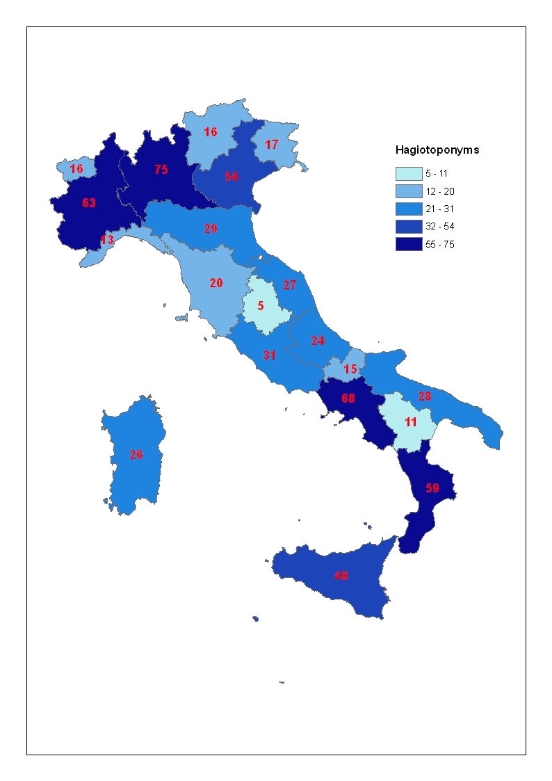
Figure 1: Map of Italy with the regional distribution of the hagiotoponyms.

The resulting distribution of the hagiotoponyms at a regional level can be found in Figure 1.

2.2 Data treatment

To exemplify the procedure, consider that we made two Tables: one with the number of inhabitants and one with the $<ATI>$ values, both in decreasing order, according to the Saint name, distinguishing between males and females. The top and bottom of each Table is shown in Table 7, 8, 9, and 10 in view of outlining the number ranges. Table 11 contains the statistical indicators computed for $<ATI>$ and population data.
To highlight the role played by each Saint, population and economic raw data have been further treated in two ways.

• Data have been cumulated over the name of the Saints as follows:

  $$ATI(x)=\sum_{j\in F(x)}ATI_{j},\qquad POP(x)=\sum_{j\in F(x)}POP_{j},\qquad\forall\,x,$$

  where $x$ denotes the name of a Saint. Thus, $F(x)$ is the set of municipalities which toponym derives from the Saint $x$, and represents the popularity of $x$. Specifically, the cardinality of $F(x)$ -denoted as $|F(x)|$- is the $frequency$ of $x$. $ATI$ and $POP$ are the intuitive notations for the ATI values and for the number of inhabitants datum, respectively. In particular, $ATI_{j}$ and $ATI(x)$ ($POP_{j}$ and $POP(x)$) represent the ATI (number of inhabitants) datum for the municipality $j$ and the Saint $x$, respectively.

• Furthermore, all data have been cumulated and next averaged to take into account the name ($x$) popularity $F(x)$ of the Saints:

  $$\overline{ATI}(x)=\frac{1}{|F(x)|}\cdot\sum_{j\in F(x)}ATI_{j},\qquad\overline{POP}(x)=\frac{1}{|F(x)|}\cdot\sum_{j\in F(x)}POP_{j},\qquad\forall\,x.$$

3 Statistical analysis of the data

First of all, we provide a description of the dataset through the main statistical indicators. Then, some specific aspects of the considered dataset will be treated, on the basis of the methodological techniques described in the Appendix.

3.1 Main statistical indicators

The computation of the main statistical indicators leads to some interesting outcomes:

• it appears that there are 91 cities with a $female$ Saint name for 31 (female) different names, as reported in Table 5 and Table 6; the most popular is Santa Maria (including Marie) occurring 23 times, much preceding Sant’Agata (12 times).
  Our statistical analysis shows that the distribution is rather skewed (skewness $\sim 3.63$) and the kurtosis $\sim 13.39$;

• from Table 5 and Table 6, it appears that there are 546 cities with one (or two) $male$ Saint name(s). The most popular is San Pietro (43 times), but San Giovanni (36 times) is not far off. There are 175 different names. (Recall restrictions, due to Cosmo and Damiani, and to Marzano and Giuseppe, as if there were 548 different cities).
  For these 548 hagiotoponyms, our statistical analysis shows that the distribution is rather skewed (skewness $\sim 4.57$) and the kurtosis $\sim 23.93$;

• there are 206 different Saints (175 males + 31 females) within the above grouping rules for 639 hagitotoponyms. This popularity ($F$) distribution is rather skewed (skewness $\sim 4.55$) and the kurtosis $\sim 24.0$.

The values of the statistical indicators provided in the above list illustrate an hagiotoponym-type of urbanization mostly related to a few very popular Saints (Pietro and Giovanni for males, Maria and Agata for females), but with a very large number of cities recalling unfrequent Saints. This is totally in line with the deep cult of very important and popular religious figures like the Virgin (Maria), the first Pope (Pietro), etc., along with widespread local traditions related to less famous Saints.

Table 11 collects the main statistical indicators related to the raw ATI and number of inhabitants data. This Table can be compared with the main statistical indicators associated to ATI and number of inhabitants when the entire set of IT cities is considered (Table 12). It is evident that the minimum values of ATI and number of inhabitants share the same magnitude order in the overall IT and hagiotoponym cases, while the maximum ones are remarkably different (the maximum of IT is much greater than that of hagiotoponyms for both the considered variables). However, IT cities are on average slightly richer and more populated than hagiotoponyms. Further information is bought by other statistical indicators: IT cities are noticeably more volatile than the set of hagiotoponyms (higher variance either for population and ATI), and exhibit also a greater level of kurtosis.
All these facts point to hagiotoponyms which describe a hypothetical IT situation when the main outliers are removed, both for the number of inhabitants as well as for the ATI.

Table 13 collects the main statistical indicators for the quantities $ATI(x)$, $POP(x)$, $\overline{ATI}(x)$, and $\overline{POP}(x)$ with respect to the independent variable $x$.
By a methodological point of view, the closest integer has been taken for $\overline{POP}(x)$. Moreover, at these levels, and thereafter, we have not distinguished between male and female names. The ratios between the number of cities having a hagiotoponym or the relative number of different Saints (in both case $\sim 0.17$) or the proportion of female Saints in the overall counting (in both cases $\sim 0.14$) are not small. Nevertheless, it is not expected that distinguishing genders would bring much to the discussion. Moreover, it should be obvious to the reader that to take into account the gender would lead to triple the number of curves, figures, columns in Tables, or Tables. However, we do not disregard the interest of such an investigation in the future, for a complementary paper.

3.2 Saints frequency regional disparities

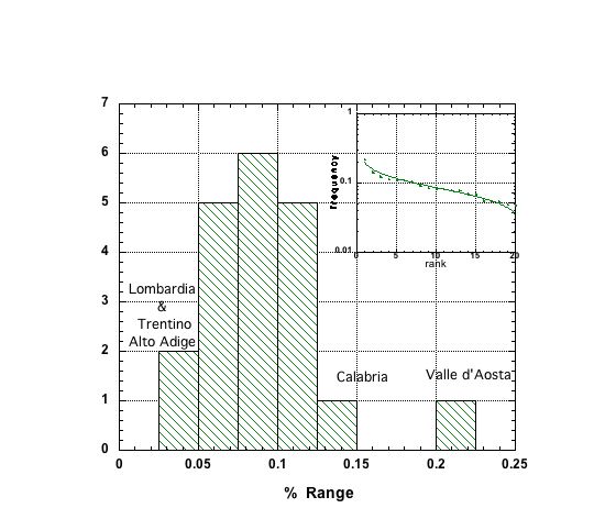
Figure 2: Histogram of the relative number of hagiotoponym cities with respect to the total number of cities in the 20 Italian regions, stressing the peculiarity of Valle d’Aosta, as an outlier and the more extreme cases Lombardia, Trentino-Alto Adige and Calabria. In an insert, the rank-size relationship is shown for the 20 regions, with a fit by the Lavalette function, Eq. (4.6); the parameter values are: $\kappa_{2}$ = 0.082; $\chi$ = 0.285; $R^{2}$ = 0.955.

It can be observed from Table 2 that, on average, there are $\sim 8\%$ hagiotoponyms in the Italian regions. However, Valle d’Aosta is an outlier in the hagiotoponym distribution, since about 22% of the municipalities contain a Saint name in that region. Recall that Valle d’Aosta is an autonomous-like region, with much historical connections with France. In fact, in France, more than 5000 municipalities, out of about 35000, i.e. about $15\%$, contain a Saint name.
In the more extreme Italian cases Lombardia and Trentino-Alto Adige are ”very poor” in hagiotoponyms: $\sim 5\%$, though these are regions in the North of IT, like Valle d’Aosta.
In contrast, Calabria, a southern region, has a much above average $\sim 14\%$ hagiotoponym content.
Note that the largest percentages of female hagiotoponyms occur in Umbria (0.6666), Sicilia (0.375) and Calabria (0.1864), as for the female/all ratio.
In contrast, the largest percentages of male/all hagiotoponyms occur in Friuli-Venezia Giulia (0.9412) and in Lazio and Valle d’Aosta (0.9375).
Basilicata has a noticeable feature: there is no female Saint name in any city.
In fine, from the search of an empirical law point of view, the finite size effect of the data is remarkably emphasized when searching for the hagiotoponym frequency distribution; see insert of Fig. 2. Taking such a finite size into account, the rank-size relationship for the 20 regions can be well reproduced by a fit with a function as Eq. (4.6). To our knowledge, the fundamental reason for the validity of such a function, in this type of considerations, is unknown, but rather ad hoc. Only mathematically plausible arguments (Naumis and Cocho, 2008) are known, but they seem hardly applicable in our case.

3.3 Saints frequency empirical distributions

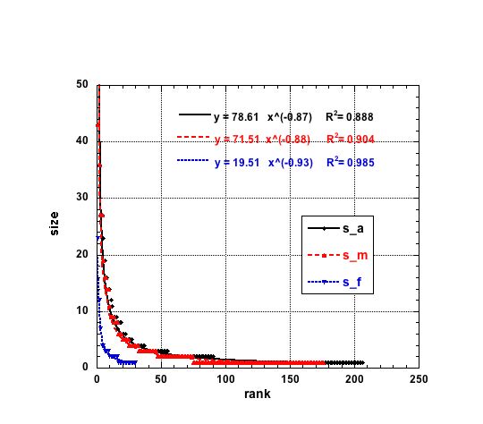
Figure 3: Display of the rank-size relationship for cities bearing a Saint name ranked in decreasing order according to their size, with corresponding power law fits as indicated; the gender (f or m) is distinguished beside the overall (a) size (s) data. The best merely hyperbolic fits are indicated.

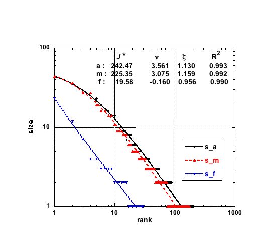
Figure 4: Log-log display of the rank-size relationship for cities bearing a Saint name ranked in decreasing order according to their ”size”, with corresponding Zipf-Mandelbrot law fits as indicated; parameters are for Eq. (4.4); the gender (f or m) is distinguished beside the overall (a) size (s) data. Note the slight king effec for Maria ($\nu\leq 0$) in the ”female data”.

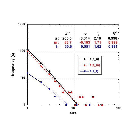
Figure 5: Log-log display of the frequency-size relationship for cities bearing a Saint name, with corresponding Zipf-Mandelbrot law fits as indicated; parameters are for Eq. (4.4); the gender (f or m) is distinguished beside the overall (a) size (s) frequency data. The most popular Saint name, in the context, is Pietro, see Table 5. Observe the convex curvature for the male data cumulative distribution function, with a slight king effect for males, due to the large number (101) of hapax Saint males, i.e. for the ”small size” region.

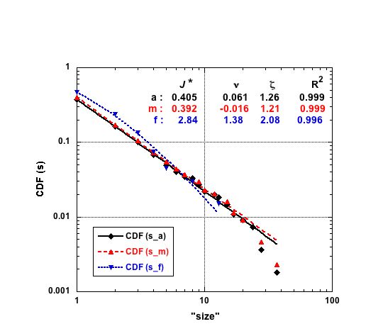
Figure 6: Log-log display of the cumulative distribution function (CDF) as a function of their ”size” for cities bearing a Saint name in decreasing order of their ”frequency”, with corresponding Zipf-Mandelbrot law fits as indicated; the gender (f or m) is distinguished beside the overall (a) size (s) data.

It has been shown here above that there are 206 different Saint names. Thereafter, a rank-size (Zipf) plot on classical axes, Fig. 3, can be presented, i.e., the number of cities, independently carrying the name of a specific Saint, ranked in decreasing order of the Saint popularity. In so doing, we are only focussing on a linguistic-like approach, as a function of the rank, i.e. how many times the Saint occurs (its ”size”) in hagiotoponym cities. The display, for the various genders and the whole data set, indicates a smoothly decreasing data, as if a Zipf law exists.
However, according to Fig. 4, displaying the same data as on Fig. 3, but on a log-log plot, the rank($r$)-size($s$) relationship for the number of times a city has the name of a Saint ($i$ $\sim$ male (m), female (f) or all (a) cases) is obviously seen to be hardly represented by a mere power law. A more appropriate fit is through a Zipf-Mandelbrot law, Eq. (4.4), with downward curving at low rank. The parameter values are given in the Figure. Nevertheless, note the slight king effect for Maria -i.e.: the distortion effect due to the outlier Maria, see Laherrère and Sornette (1998)- ($\nu\leq 0$). Note also that the power law decay at high rank is very similar for each gender, with an exponent ($\zeta$) close to 1. Such fits are rather remarkable since the regression coefficient $R^{2}\geq 0.99$.
A log-log display of the frequency-size relationship, Eq. (4.3), i.e. the frequency of the size, for the Italian cities bearing a Saint name, is shown in Fig. 5. The corresponding fits with a Zipf-Mandelbrot law, Eq. (4.4), are indicated; the gender ($f$ or $m$) is distinguished beside the overall (a) size (s) frequency data. The fits are rather remarkable, since $R^{2}\geq 0.99$. It should not be surprising in such a plot to observe a slight king effect for the male case, nor the largest value of the $\zeta$ exponent in the all Saint case, due to the small influence of the (rare) high size Saints.
A final plot, in examining the given Saint size distributions is through a log-log display of the cumulative distribution function (CDF) as a function of the ”size” relationship, Eq. (4.5), i.e. Fig. 6. Recall that cities bearing a Saint name are listed in decreasing order of their frequency. The regression coefficient is again very high for fits with a Zipf-Mandelbrot law, Eq. (4.4). A technical point is in order concerning the female data fit. The latter is very unstable due to the small number of points, i.e. 7. The parameter values much depend on the initial conditions imposed in the Levenberg-Marquardt algorithm. This is due to the large number of approximately equivalent minima in the parameter space; this unavoidable fact is well known (see Herzel et al., 1994, Goldstein et al., 2004, Clauset et al., 2009, Rawlings et al., 1998).

3.4 Population size considerations

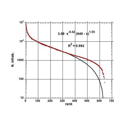
Figure 9: Semi-log display of the Number of inhabitants in the 639 (637 + 2; see text) Saints generating Italian hagiotoponyms, - cities ranked in decreasing order of the number of inhabitants; a fit by a Lavalette function shows a convincing fit for $r\leq 350$.

The number of inhabitants in the 639 hagiotoponym cities is presented on a linear-linear plot in Fig. 7. Visually, this looks like displaying a smoothly, hyperbolic-like, decaying data, with an exponent close to 1. However, the $R^{2}$ value is pretty low, i.e. $\sim 0.54$. Alas, as better seen in Fig. 8, there is no nice simple fit, by an empirical law with few free parameters.
Indeed, Fig. 8 presents a log-log plot for the rank-number of inhabitants in the 639 Italian hagiotoponym cities. Visually, from the data scattering, it cannot be expected that a simple empirical law can be found: four simple laws are indicated, but do not lead to a convincingly interesting regression coefficient. The Zipf-Mandelbrot law has a $R^{2}\sim 0.98$, but is far from being visually appealing at high rank. It can be concluded, at this stage, that the sampling is far from a random one.
Note that these simple fits for the ”all Saints” case (Fig. 7 and Fig. 8) are not nice enough to suggest a decomposition between males and females in further work.
In view of the change in curvature of the data near the middle of the rank range, it is inappropriate to consider a fit by a power law or any other purely convex function. Instead, like for Fig. 1 insert case, it seems that a fit by a 3-parameter function with inflection point, as that given in Eq. (4.7) in Appendix, is more appealing. This is shown in Fig. 9, on a semi-log display of the number of inhabitants in the 639 Italian cities wearing a Saint name, - cities ranked in decreasing order of the number of inhabitants; a fit by such a function shows a convincing $R^{2}\sim 0.992$. Moreover, the fit for $r\leq 350$ is quite visually appealing.
These results can be compared with what the overall 8092 IT cities say.
There is evident presence of outliers at a high rank, as the histogram in Fig. 10 noticeably puts in evidence. This fact is further confirmed by the fits for IT, which seem to be more of high quality when outliers are removed. In this respect, the comparison between the best 3-parameters Lavalette fit in the two cases of all 8092 cities and of removal of the 80 highest rank cities is pretty informative, being the latter more visually appealing than the former (see Figures 11 and 12).
Also the case of low rank is quite interesting. Fig. 13 shows that the low rank IT cities are nicely fitted by a 3-parameters Lavalette curve, with $R^{2}\sim 0.986$.
To conclude, by ranking cities with respect to the number of inhabitants, the sample of hagiotoponym cities behaves closely to the overall IT cities when outliers are removed.

3.5 Economic considerations

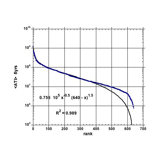
Figure 15: Semi-log display of the the average ATI over 5 years for the 639 (637 + 2; see text) Saints generating Italian hagiotoponyms, cities ranked in decreasing order of their ATI; a fit by a Lavalette function shows a convincing fit for $r\leq 350$.

The $<ATI>$ of all the 639 Italian cities containing a Saint name over the period 2007-2011 has been displayed on log-log axes in Fig. 14. It is seen on this figure that simple laws, as those tested, i.e. power, exponential, log, do not point to a plausibly simple empirical relationship.
In fact, in view of the change in curvature of the data near the middle of the rank range, it is inappropriate to consider a fit by a power law or any other purely convex function. Instead, like for Fig. 1 insert case, it seems that a fit by a 3-parameter function with inflection point, as that given in Eq. (4.7), is more appealing. A semi-log display of the $<ATI>$ the 639 Italian hagiotoponym cities, cities ranked in decreasing order of their ATI is shown in Fig. 15. A fit by such a 3-parameter free function shows a convincing fit for $r\leq 350$, and an acceptable $R^{2}\sim 0.989$. The latter is smaller than in the case of the population size, in Fig. 9, but the exponents seem quite similar.

Also in this case, the comparison between the outcomes of the economic analysis of the hagiotoponyms and the one related to the IT cities might be of some usefulness.
At this level, we refer the reader to Cerqueti and Ausloos (2015), where rank-size rules are applied at a national as well as at a regional level for cities in IT. The size is given by the ATI, and data are disaggregated on the basis of municipal unit.
Cerqueti and Ausloos show that IT national economic data seems to be well described by a 3-parameters Lavalette curve, even if the distortion effect due to the presence of outliers is of high magnitude. This is the so-called king and vice-roy effect, see Section 4.2 in the cited paper. For what concerns the validity of Zipf-Mandelbrot law, the hagiotoponym sample behaves according to the overall IT and to the majority of IT regions, in that it statistically fails in all the cases, being Lazio region a remarkable exception.
Hence, we can reasonably state that the set of hagiotoponym cities proxies IT cities without outliers, when ATI is considered in the context of rank-size rules.

3.6 Study of the correlations

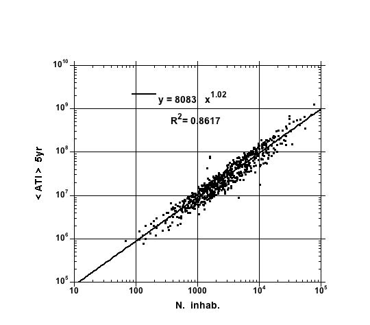
Figure 16: Log-log display of the scatter plot for the averaged over 5 years ATI and the number of inhabitants for the 639 (637 + 2; see text) Saints generating Italian hagiotoponyms, with the best power law fit.

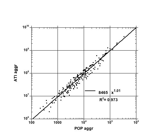
Figure 17: Log-log display of the scatter plot of the cumulated averaged over 5 years ATI and the cumulated Number of inhabitants for the 206 different Saints, with the best power law fit.

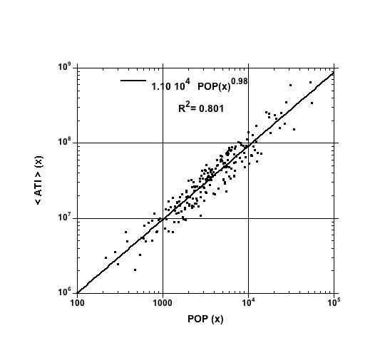
Figure 18: Log-log display of the scatter plot of the averaged over 5 years ATI $\overline{ATI}(x)$ and the Number of inhabitants $\overline{POP}(x)$ for the 206 different Saints, reduced at the frequency (popularity) of the Saint, with the best power law fit.

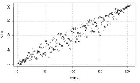
Figure 20: Display of the scatter plot of ranks for $ATI(x)$, i.e. the cumulated averaged over 5 years ATI, and the cumulated number of inhabitants ($POP(x)$) for the 206 different Saints.

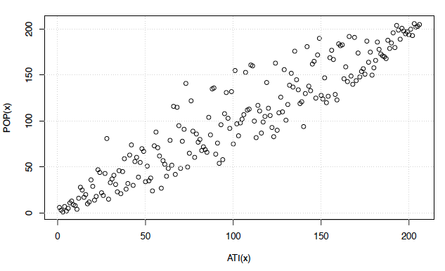
Figure 21: Display of the scatter plot of ranks for $ATI(x)$, i.e. the averaged over 5 years ATI and the number of inhabitants ($POP(x)$) for the 206 different Saints, reduced by the frequency (popularity) of the Saint, i.e. $\overline{POP}(x)$ and $\overline{ATI}(x)$.

In view of the above findings, considering that similar empirical laws seem to hold for relations between the city population, Fig. 9, and the city wealth, Fig. 15, as a function of the rank in the relevant variable, it seems of interest to search whether such ranks are correlated. Such an answer is obtained from so called scatter plots (see Bradley, 2007), which allows to have some insight in the correspondence between data lists when the measures themselves are of less interest than their relative ordering importance.
First, a log-log display of the scatter plot for the $<ATI>$ and the number of inhabitants, for the 639 Italian hagiotoponym cities, is presented in Fig. 16. The best power law fit indicates a loosely compact set of points along a quasi linear function. A correlation seems plausible, but there are a few outliers.
Next, the corresponding scatter plot for the cumulated variables, i.e. $ATI(x)$ and $POP(x)$, thus for the 206 Saints, can be observed in Fig. 17 on log-log axes. Again, a fine power law with an exponent close to 1 is found.
Third, Fig. 18 is the corresponding log-log display of the scatter plot of the averaged over 5 years ATI and the number of inhabitants, in cities corresponding to the 206 Saints, but when reduced as a function of the frequency (popularity) of the Saint, i.e. $\overline{ATI}(x)$ and $\overline{POP}(x)$. Again the exponent of such a power law fit is close to 1.
The regression coefficient is the highest for the cumulated data, as should be expected. However, the $R^{2}$ is much lower ($\sim 0.8$) in the latter case, indicating much scattering, whence a rather strong deviation from a perfectly correlated popularity (frequency) effect.
In order to quantify some correlation in two (necessarily equal size) sets, e.g., between population and ATI data, the Kendall’s $\tau$ rank measure (Kendall, 1938) is usefully calculated.
First of all, it is important to note that $N$= 206 implies $p+q=21115$, when there is no overlap, being $p$ and $q$ the number of concordant and discordant pairs, respectively. However, in the present case, two hapax Saints (Bassano and Sosti) have the same cumulated number of inhabitants (2209), whence $p+q$= 21114.
The relevant data, i.e. the Kendall $\tau$, Eq. (4.8), and correlation statistics of ranking order between (i) $\overline{POP}(x)$ and $\overline{ATI}(x)$; (ii) $POP(x)$ and $F$; (iii) $ATI(x)$ and $F$; (iv) $\overline{POP}(x)$ and $F$; (v) $\overline{ATI}(x)$ and $F$, for 206 Saints ($x$), with notations as in the text, are given in Table 15. For a visual inspection of the correlations among the variables belonging to this set of data, of some usefulness can be Figs. 20 and 21.
The marked variations between the various $\tau$ coefficients allow interesting observations. First of all, one can compute the Kendall coefficient between the number of inhabitants and $<ATI>$ for the 637 hagiotoponym cities, and obtain $\simeq 0.81$. Admitting that there might likely be some different wealth regime of the inhabitants in the various cities, it is bona fide expected that the total $<ATI>$ of a city would be somewhat in direct (simple) relation with the number of inhabitants. In fact, there are variations in the $<ATI>/N$ (ATI per inhabitants) values. For this, we found: mean $\sim 9813$; median $\sim 9593$; standard deviation $\sim 3893$. However the relative pair ranking concordance ratio $p/q$ is $\sim 9.7$. It maybe concluded that there is a high concordance.
It is here interesting to point out the analogies and disparities among hagiotoponyms and IT when dealing with the Kendall rank correlation, being the variables under scrutiny ATI and number of inhabitants.
The Kendall $\tau$ for the case of IT cities is reported in Table 14. It is immediate to check that Kendall $\tau$ is substantially the same in the case of hagiotoponyms ($\tau\sim 0.849$) and IT ($\tau\sim 0.850$). From this, it can be concluded that there is a strong regularity in the correlations between the two types of city ranking in IT. Moreover, it is also important to stress that the discrepancies between IT and hagiotoponyms can be found in the number of inhabitants and in the ATI, and not in how the corresponding ranks are associated. This further confirms what already found for the relationship between IT and Saint cities.
The matter is quite different for the cumulated data rank correlations observed at the Saint level: $\tau\simeq 0.850$ or $\tau\simeq 0.788$, for which $p/q\sim 12.35$ or $p/q\simeq 8.44$, either for the total cumulated data per Saint of for the reduced value taking into account the Saint popularity: columns (i) and (ii) in Table 15. This huge variation in $p/q$ is, surprisingly, pointing to a redistribution of the ranks, following some sort of randomization.
The effect is amplified when the correlations with the Saint popularity are examined: in this case, $\tau\sim 0.510$ for $POP(x)$, with the ratio $p/q\sim 3.08$, and a similar $\tau\sim 0.518$ is found for the rank correlation between $ATI(x)$ with respect to the frequency $F$ of a Saint. In the latter case, the ratio $p/q\sim 3.15$ (see columns (iii) and (iv) in Table 15). Therefore, it can be concluded that the cumulated population of cities for a given Saint is far from being positively correlated with the Saint popularity.
When taking into account the Saint popularity and the cumulated data of cities into the Saint level, we have that the ranking correlations with respect to the Saint popularity leads to a very small $\tau\sim 0.068$ or $\tau\sim 1.02$. Note that the ratios $p/q$ are $\sim 1.15$ and $\sim 1.22$; see columns (v) and (vi) in Table 15. From a purely statistical perspective, this result is very close to prove an independence of the rank sets.
Finally, on one hand, this indicates how careful one should be in drawing conclusions from one statistical indicator only. On the other hand, it points to a ”Saint” effect, either positive or negative, depending on the considered variable.

4 Conclusion

In summary, let us note that the objectives of the study were to describe the Italian society when referring to a key aspect of it: the cult of catholic Saints and its reflection on the toponyms of the Italian cities. With this aim, we have found that:

• there exists an exhaustive list of cities in IT whose toponym is a derivation of a human Saint name. This requested some linguistic approach beside some religiosity filter. The resulting dataset can be used for subsequent studies dealing with related problems;

• there exists a rather simple empirical law for the distribution of Saint Names as hagiotoponym of cities, in particular in IT, and who are the hapax Saints;

• there exists a rather simple empirical law about the distribution of population sizes for such cities;

• there exists a rather simple empirical law about the wealth distribution, for such cities, measured through their Aggregated Income Tax;

• there exists some correlation between such data. Specifically, there is a high concordance between the ranking of the average ATI and of the population for the hagiotoponyms.

• there are qualitatively reasonable causes which can be given for the findings.

The empirical laws are not trivial ones, thereby proposing further mathematical investigations on them. This remark holds for the city population and the ATI. Correlations exist between both variables, but with some loose ties because of the outliers.
Our conclusion on city population $vs.$ ATI correlations tends to indicate that these cities with hagiotoponyms are not drastically different from those in the rest of IT. In particular, it seems that hagiotoponym cities may represent a proxy of the overall IT cities when outliers are removed, both at an economic as well as a demographic level. Moreover, the rank-rank relationship between ATI and number of inhabitants – obtained by employing the Kendall $\tau$ – leads to a robust outcome of concordance. The results on Saint popularity, in fine, seem to indicate a lack of correlations between the latter and the two main variables which we have examined.
On (v), further explanations are needed. Let us distinguish females and male names. The most important cult to have developed in christianity is that of the Virgin Mary, whence St. Maria is naturally an appealing Saint name for providing some cult in some city, and having given the name to several places.
Yet, it seems interesting that she is less popular than Pietro and Giovanni, who both were the closest apostles to Jesus, according to christian tradition. Interestingly Martino comes third, before Giorgio. Martin is also very popular in France and other countries, where his name is usually more popular (Ausloos, unpublished) than Giovanni (Jean) and Pietro (Pierre). Giorgio’s 4th place is interesting: his name occurs much in IT, but also all over Europe. The popularity of George is likely due to the religious role played by Saint George, who killed dragons which synthesized the devil and its hell.
Agatha, as the second most popular female Saint is also interesting. She represents one of the most important martyr of the sicilian christianity: she is venerated at least as far back as the sixth century, ”because” she had her breasts cut off, whence of interest for cults by women in order to produce gynecological miracles. Why men, usually leading the populations at those early Christian times, would give her name to a city is nevertheless an open question.

Appendix A: Methodological instruments

This Appendix contains a few lines on the theoretical background of the empirical laws, along with an explanation of the Kendall $\tau$, for the reader convenience.

Formulas for fit

Zipf (1949) had observed that a large number of size distributions, $N_{r}$ can be approximated by a simple scaling (power) law $N_{r}=N_{1}/r$, where $r$ is the ranking parameter, with $N_{r}\geq N_{r+1}$, with obviously $r<r+1$.
A more flexible equation, with two parameters, reading

$$N_{r}=\cfrac{N_{1}}{r^{\alpha}},$$ (4.1)

is called the rank-size scaling law and has been often applied to city sizes. The particular case ${\alpha}=1$ is thought to represent a desirable situation, in which forces of concentration balance those of decentralization. Such a case is called the rank-size rule. The interested reader is referred to Gabaix (1999), Gibrat (1957), Laherrère and Sornette (1998), Ausloos (2013), Fairthorne (1969), Adamic (2005), Shannon (1948), Vitanov and Dimitrov (2014), McKean et al. (2009), Wolfe (2009, 2010), Lin (2010), Wieder (2009). Hence, the rank-size relationship has been frequently identified and sufficiently discussed to allow us to base much of the present investigation on such a simple law. This may be ”simply” because the rank-size relationship can be applied to a wide range of specific situations (see Martìnez-Mekler et al., 2009) and Zipf’s law obtained in different models: one example is tied to the maximization of the entropy concept in Chen (2012); another stems from the law of proportionate effect, so called Gibrat’s law (Gibrat, 1957).
Thus, let us express Zipf’s law, in other words: the rank-frequency relationship, i.e. the relationship between the number $f$ (frequency) of the occurrence of an ”event” and its rank $r$ (Hill, 1974), consists of an inverse power law:

$$f\sim r^{-\alpha}.$$ (4.2)

A display of the rank-size (or rank-frequency, two names for the same concept) relationship for cities bearing a Saint name ranked in decreasing order according to their ”frequency”, Eq. (4.2), is shown in Fig. 4. The best (least square) corresponding power law fits are indicated; the gender (f or m) is distinguished beside the overall (a) size (s) data. It can be observed that the power law fits look quite acceptable, being almost perfect in the ”female case”.
Another law is attributed to Zipf : the size-frequency relationship, i.e.: the link between the frequency $f$ and the size $s$ of an ”event”, is also in this case an inverse power law:

$$f\sim s^{-\lambda}.$$ (4.3)

Of course, deviations from the simple law often occur, as illustrated through Fig. 8 and Fig. 14. In fact, there is no obligation for the size-frequency data to be enveloped by a purely convex or purely concave function (Egghe and Waltman, 2011). A so called ”king effect” (Lahèrrere and Sornette, 1998) i.e. a sharp upturn at low $r$ values often exists. A leveling off at low $r$, the queen effect can also occurs, as in Fig. 4 (see also Ausloos, 2013). In such a case, a Zipf-Mandelbrot-like (ZM), sometimes called Bradford-Zipf-Mandelbrot-like (BZM), law

$$J(r)=\frac{J^{*}}{(\nu+r)^{\zeta}},$$ (4.4)

might be considered as more realistic (Fairthorne, 1969). It implies three parameters ($J^{*}$, $\nu$ and $\zeta$).
Moreover, it can also be asked how many times one can find an ”event” greater than some size $s$, i.e. within the size-frequency relationship. Pareto (1896) found out that the the cumulative distribution function of such events follows an inverse power of $s$, or in other words,

$$P\;[Y>s]\sim s^{-\kappa},$$ (4.5)

where $Y$ is the random variable of the size, $P$ a probability measure and $\kappa$ a scalar. Again, this is quite an approximation, as illustrated through Fig. 6.
It is important to observe that the Yule-Simon distribution can be used to reproduce a Zipf law, but it introduces an exponential cutoff in the upper tail (Rose et al., 2002). The stretched exponentials (Lahèrrere and Sornette, 1998) and log-normal distributions (Montroll and Shlesinger, 1983) usually reproduce one of the tails but not the other. Usually, such deviations do not change in a dramatic way the correlation coefficient since the tails do not have a great impact upon this coefficient. Moreover, such distributions assume along (infinite) tail which is antagonistic to the concept of finite sizes, when there is a true maximum rank $r_{M}$.
When an inflection point occurs, the 2-parameter form, so called Lavalette function (Lavalette, 1966), of the rank-frequency (or rank-size) relationship reads:

$$g_{2}(r)=\kappa_{2}\;\left[\frac{N\;r}{N-r+1}\right]^{-\chi};$$ (4.6)

its simple generalization into a 3-parameter free function (Popescu et a., 1997, Popescu, 2003, Mansilia et al., 2007, Ausloos, 2014b) is

$$\;\;g_{3}(r)=\kappa_{3}\;\frac{(N\;r)^{-\gamma}}{(N-r+1)^{-\xi}}.$$ (4.7)

Note also that the role of $r$ as independent variable in Zipf’s law. Specifically, Eq. (4.1) is taken by the ratio $r/(N-r+1)$ between the descending and the ascending ranking numbers. The semi-logarithmic graph shows a reverse sigmoidal S-shape (or an inverse N-shape) which cannot be provided by Zipf’s law. By the way, in a double-logarithmic diagram the downwards deviation from the Zipf’s straight line at high rank is much emphasized.
More complicated forms with many more parameters generalize the Lavalette form (see Ausloos, 2014a, 2014b and Voloshynovska, 2011). They provide better fits, but seem of no special interest here.
It is fair to mention that the mere hyperbolic form has some sound mathematical, statistical and physical basis. The BZM form, Eq.(4.4), and the Lavalette functions have not yet received a sound physical basis to our knowledge though some mathematical insight has been provided (Naumis and Cocho, 2008).

Kendall $\tau$ coefficient

The Kendall’s $\tau$ measure, introduced in Kendall (1938) compares the number of concordant pairs $p$ and non-concordant pairs $q$ through

$$\tau=\;\frac{p-q}{p+q}.$$ (4.8)

Of course, $p+q=N(N-1)/2$, where $N$ is the number of measures, when there is no doubt about measure rank (i.e., no rank overlap). For large samples, it is also common to measure

$$Z=\frac{\tau}{\sigma_{\tau}}\;\equiv\frac{\tau}{\sqrt{\frac{2(2N+5)}{9N(N-1)}}}.$$ (4.9)

similar to the classical one, when the distribution can be approximated by the normal distribution, with mean zero and variance, - in order to emphasize the coefficient $\tau$ significance. From a purely statistical perspective, under the null hypothesis of independence of the rank sets, such a sampling would have an expected value $\tau$ and $Z$ = 0.

A website (Wessa, 2012) allows $\tau$ immediate calculation.

Appendix B: Figures and Tables

Tables

Municipality	Saint name	Province	Region
Guardia Sanframondi	FREMONDO	BN	CAMPANIA
Sampeyre	PIETRO	CN	PIEMONTE
Samugheo	MICHELE	OR	SARDEGNA
Sanfré	IFFREDO	CN	PIEMONTE
Sanfront	FRONTONE	CN	PIEMONTE
Sangiano	GIOVANNI	VA	LOMBARDIA
Sanremo	ROMOLO	IM	LIGURIA
Santeramo in Colle	ERASMO	BA	PUGLIA
Santhià	AGATA	VC	PIEMONTE
Santomenna	MENNA	SA	CAMPANIA
Santorso	ORSO	VI	VENETO
Santu Lussurgiu	LUSSORIO	OR	SARDEGNA
Sanzeno	SISINNIO	TN	TRENTINO ALTO ADIGE

Table 1: So called accepted strange cases: municipality (listed in alphabetical order) and corresponding Saint name, with the province or region membership. The (only) female Saint is reported in italic. Very interesting are the cases of Sanremo in Liguria and Sanzeno in Trentino Alto Adige. Unexpectedly Sanremo, which reasonably should refer to Saint Remo, points actually to Saint Romolo, bishop of Genua in the IX century. Indeed, a Saint named Remo does not exist, and Sanremo is a dialectal contraction of San Rœmü, which means Romolo. Sanzeno who might let the reader think about Saint Zenone derives actually from the martyr Sisinnio.

REGION	N. Cities	Hagiotop.	Saint freq.	Males	Females
ABRUZZO	305	24	24	18	6
BASILICATA	131	11	11	11	0
CALABRIA	409	59	59	48	11
CAMPANIA	551	68	68	59	9
EMILIA ROMAGNA	348	29	29	25	4
FRIULI VENEZIA GIULIA	218	17	17	16	1
LAZIO	378	31(*)	32	30	2
LIGURIA	235	13	13	12	1
LOMBARDIA	1544	75	75	67	8
MARCHE	239	27	27	25	2
MOLISE	136	15	15	13	2
PIEMONTE	1206	63	63	59	4
PUGLIA	258	28(*)	29	26	3
SARDEGNA	377	26	26	20	6
SICILIA	390	40	40	25	15
TOSCANA	287	20	20	17	3
TRENTINO ALTO ADIGE	333	16	16	14	2
UMBRIA	92	5	5	3	2
VALLE D’AOSTA	74	16	16	15	1
VENETO	581	54	54	45	9
Total	8092	637	639	548	91

Table 2: Summary Table with the hagiotoponym cities in IT. Data are disaggregated at the regional level, in the alphabetical order for regions. The discrepancy between the number of hagiotoponyms (637) and the Saints ”frequency” (639) is due to the presence of cities with a name containing two Saints: Cosma and Damiano, Marzano and Giuseppe, see $(^{*})$ in the Table and the discussion in the text. All data refer to 2011.

Group of linguistic transformation	Saint name
Basile, Basilio	BASILE
Biagio, Biase	BIAGIO
Casciano, Cassiano	CASCIANO
Cesario, Cesareo	CESARIO
Cosma, Cosmo	COSMO
Donato, Doná	DONATO
Fedele, Fele	FEDELE
Felice, Fili	FELICE
Floriano, Fiorano	FLORIANO
Floro, Fior	FLORO
Gemini	GEMINE
Genesio, Ginesio	GENESIO
Lorenzo, Lorenzello	LORENZO
Maria, Marie, Madonna, Notre-Dame	MARIA
Michele, Sammichele	MICHELE
Nazzaro, Nazario, Sannazzaro	NAZZARO
Nicandro, Sannicandro	NICANDRO
Nicola, Niccoló, Nicolao, Nicoló, Sannicola	NICOLA
Paolo, Polo, sampolo	PAOLO
Pietro, Piero, Pier, sampiero, Pietrangeli	PIETRO
Quirico, Chirico	QUIRICO
Stefano, Stino	STEFANO
Zenone, Zeno	ZENONE

Table 3: Linguistic transformations and corresponding Saint name. The only female Saint name so concerned is Maria, as emphasized in italic.

Municipality	Saint name
San Candido/Innichen	CANDIDO
Santa Cristina Valgardena/St. Christina in Gröden	CRISTINA
Senale-San Felice/Unsere Liebe Frau im Walde-St. Felix	FELICE
San Genesio Atesino/Jenesien	GENESIO
San Leonardo in Passiria/St. Leonhard in Passeier	LEONARDO
San Lorenzo di Sebato/St. Lorenzen	LORENZO
San Martino in Badia/St. Martin in Thurn	MARTINO
San Martino in Passiria/St. Martin in Passeier	MARTINO
San Pancrazio/St. Pankraz	PANCRAZIO
Antey-Saint-André	ANDREA
Challand-Saint-Anselme	ANSELMO
Saint-Christophe	CRISTOFORO
Saint-Denis	DENIS
Pré-Saint-Didier	DIDERO
Rhêmes-Saint-Georges	GIORGIO
Gressoney-Saint-Jean	GIOVANNI
Saint-Marcel	MARCELLO
Rhêmes-Notre-Dame	MARIA
Pont-Saint-Martin	MARTINO
Saint-Nicolas	NICOLA
Saint-Oyen	OYEN
Saint-Pierre	PIETRO
Saint-Rhémy-en-Bosses	RHEMY
Saint-Vincent	VINCENZO
Challand-Saint-Victor	VITTORIO

Table 4: The set of 9+16 toponyms in foreign (= non-Italian) language and the corresponding Saint name (in Italian). They belong to Valle d’Aosta (16 cities) and Trentino Alto Adige (9 cities). Female Saints are reported in italic.

SAINT NAME	Freq.	SAINT NAME	Freq.	SAINT NAME	Freq.
PIETRO	43	$CRISTINA$	4	$ANASTASIA$	2
		$MARGHERITA$	4	$DOMENICA$	2
GIOVANNI	36			$EUFEMIA$	2
		BARTOLOMEO	4	$GIUSTINA$	2
MARTINO	27	CASCIANO	4	$MARINA$	2
GIORGIO	27	DAMIANO	4	$SOFIA$	2
		GENESIO	4	$TERESA$	2
$MARIA$	23	GERMANO	4
		GIULIANO	4	CARLO	2
STEFANO	19	GIUSEPPE	4	COSMA	2
		MARCELLO	4	CONSTATINO	2
NICOLA	16			COSTANZO	2
PAOLO	16	$ANNA$	3	CRISTOFORO	2
		$CATERINA$	3	DANIELE	2
LORENZO	14	$ELENA$	3	DEMETRIO	2
VITO	14	$VITTORIA$	3	DIDERO	2
				EGIDIO	2
$AGATA$	12	ALESSIO	3	ELPIDIO	2
		AMBROGIO	3	EUSANIO	2
MICHELE	11	BASILE	3	FEDELE	2
		CESARIO	3	FERDINANDO	2
ANDREA	9	CIPRIANO	3	FERMO	2
GIACOMO	9	COLOMBANO	3	FLORIANO	2
MARCO	9	ELIA	3	FLORO	2
		GERVASIO	3	GIUSTO	2
$LUCIA$	7	MANGO	3	ILARIO	2
		MARZANO	3	LEONARDO	2
BENEDETTO	8	ROCCO	3	MAURIZIO	2
FELICE	8	SEBASTIANO	3	NICANDRO	2
MAURO	8	SECONDO	3	PANCRAZIO	2
		SEVERINO	3	POTITO	2
ANTONIO	6			SIRO	2
BIAGIO	6			TEODORO	2
GREGORIO	6			URBANO	2
				VALENTINO	2
DONATO	5			VITTORE	2
NAZZARO	5
QUIRICO	5
VINCENZO	5
ZENONE	5

Table 5: Different Saints names in alphabetical order with frequency (Freq.), or ”popularity”, when occurring more than once in hagiotoponyms; distinguishing males (74) from females (16) whose names are italicized. Recall that the underlined Saints should count for 1/2 when counting the number of cities.

ANATOLIA	ABBONDIO	FIDENZIO	ORSO
BRIGIDA	AGAPITO	FILIPPO	OYEN
CESAREA	AGNELLO	FRANCESCO	PATRIZIO
ELISABETTA	AGOSTINO	FRATELLO	PELLEGRINO
FIORA	ALBANO	FREMONDO	PIO
FLAVIA	ALESSANDRO	FRONTONE	PONSO
GIULETTA	ALFIO	GAVINO	POSSIDONIO
GIUSTA	ANSELMO	GEMINE	PRISCO
MARINELLA	ANTIMO	GENNARO	PROCOPIO
NINFA	ANTIOCO	GILLIO	PROSPERO
ORSOLA	ANTONINO	GIMIGNANO	QUIRINO
PAOLINA	APOLLINARE	GIULIO	RAFFAELE
SEVERINA	ARPINO	GIUSTINO	RHEMY
SUSANNA	ARSENIO	GODENZO	ROBERTO
VENERINA	BASSANO	IFFREDO	ROMANO
	BELLINO	IPPOLITO	ROMOLO
	BENIGNO	LAZZARO	RUFO
	BERNARDINO	LEO	SAVINO
	BONIFACIO	LEUCIO	SEVERO
	BOVO	LUCA	SISINNIO
	BRUNO	LUCIDO	SOSSIO
	CALOGERO	LUPO	SOSTENE
	CANDIDO	LUSSORIO	SOSTI
	CANZIAN	MAGNO	SPERATE
	CATALDO	MAMETTE	TAMMARO
	CIPIRELLO	MARCELLINO	TOMASO
	CLEMENTE	MASSIMO	VENANZO
	CONO	MENNA	VENDEMIANO
	DALMAZZO	MINIATO	VERO
	DENIS	OLCESE	VICINO
	DOMENICO	OMERO	VITALE
	DONACI	OMOBONO	VITALIANO
	DORLIGO	ONOFRIO	VITTORIO
	ERASMO	ORESTE

Table 6: Hapax Saints: first column collects the 15 females (in italic), while the other columns list the 101 males.

St. Name	Sex	Toponym	REGION	N. inhab.
Giovanni	M	Sesto San Giovanni	LOMBARDIA	76970
Elena	F	Quartu Sant’Elena	SARDEGNA	69295
Severo	M	San Severo	PUGLIA	55053
Romolo	M	Sanremo	LIGURIA	53617
Benedetto	M	San Benedetto del Tronto	MARCHE	46988
Giorgio	M	San Giorgio a Cremano	CAMPANIA	45058
Donato	M	San Doná di Piave	VENETO	40691
Giuliano	M	San Giuliano Milanese	LOMBARDIA	35924
Antimo	M	Sant’Antimo	CAMPANIA	33950
Maria	F	Santa Maria Capua Vetere	CAMPANIA	32603
Lazzaro	M	San Lazzaro di Savena	EMILIA ROMAGNA	31 183
Giuliano	M	San Giuliano Terme	TOSCANA	31 157
Donato	M	San Donato Milanese	LOMBARDIA	31 037
Miniato	M	San Miniato	TOSCANA	27633
Giovanni	M	San Giovanni Rotondo	PUGLIA	27371
Giuseppe	M	San Giuseppe Vesuviano	CAMPANIA	27310
Giovanni	M	San Giovanni in Persiceto	EMILIA ROMAGNA	27051
Erasmo	M	Santeramo in Colle	PUGLIA	26662
Elpidio	M	Porto Sant’Elpidio	MARCHE	25354
Anastasia	F	Sant’Anastasia	CAMPANIA	25082
…	…	…	…	…

Table 7: Top 20 hagiotoponym cities in IT, in terms of number of inhabitants. Females are italicized; hapax Saints are underlined.

St. Name	Sex	Toponym	REGION	N. inhab.
…	…	…	…	…
Paolo	M	San Paolo Albanese	BASILICATA	313
Eufemia	F	Sant’Eufemia a Maiella	ABRUZZO	304
Vicino	M	Poggio San Vicino	MARCHE	297
Ponso	M	San Ponso	PIEMONTE	279
Elena	F	Sant’Elena Sannita	MOLISE	272
Michele	M	Olivetta San Michele	LIGURIA	225
Oyen	M	Saint-Oyen	VALLE D’AOSTA	217
Giovanni	M	San Giovanni Lipioni	ABRUZZO	213
Biagio	M	San Biase	MOLISE	209
Giorgio	M	Rhemes-Saint-Georges	VALLE D’AOSTA	196
Benedetto	M	San Benedetto Belbo	PIEMONTE	193
Giovanni	M	Sale San Giovanni	PIEMONTE	178
Vito	M	Celle di San Vito	PUGLIA	172
Lucia	F	Villa Santa Lucia degli Abruzzi	ABRUZZO	144
Paolo	M	San Paolo Cervo	PIEMONTE	142
Giorgio	M	San Giorgio Scarampi	PIEMONTE	131
Benedetto	M	San Benedetto in Perillis	ABRUZZO	130
Maria	F	Rhemes-Notre-Dame	VALLE D’AOSTA	114
Stefano	M	Santo Stefano di Sessanio	ABRUZZO	114
Giuseppe	M	Rima San Giuseppe	PIEMONTE	68

Table 8: Bottom 20 hagiotoponym cities in IT, in terms of the number of inhabitants. Females are italicized; hapax Saints are underlined.

Name	Sex	Toponym	REGION	Average ATI
Giovanni	M	Sesto San Giovanni	LOMBARDIA	1240078983
Elena	F	Quartu Sant’Elena	SARDEGNA	723839629
Donato	M	San Donato Milanese	LOMBARDIA	681177081
Romolo	M	Sanremo	LIGURIA	650834136
Lazzaro	M	San Lazzaro di Savena	EMILIA ROMAGNA	589480816
Benedetto	M	San Benedetto del Tronto	MARCHE	558246404
Donato	M	San Donà di Piave	VENETO	543509572
Giuliano	M	San Giuliano Milanese	LOMBARDIA	507215120
Giuliano	M	San Giuliano Terme	TOSCANA	458205438
Giorgio	M	San Giorgio a Cremano	CAMPANIA	427785711
Giovanni	M	San Giovanni in Persiceto	EMILIA ROMAGNA	396583755
Miniato	M	San Miniato	TOSCANA	350427626
Severo	M	San Severo	PUGLIA	346136016
Pietro	M	Castel San Pietro Terme	EMILIA ROMAGNA	316883099
Giovanni	M	San Giovanni Lupatoto	VENETO	312392144
Maria	F	Santa Maria Capua Vetere	CAMPANIA	304644801
Mauro	M	San Mauro Torinese	PIEMONTE	302387316
Elpidio	M	Porto Sant’Elpidio	MARCHE	247343572
Casciano	M	San Casciano in Val di Pesa	TOSCANA	238256972
Bonifacio	M	San Bonifacio	VENETO	236053538
…	…	…	…	…

Table 9: Top 20 hagiotoponym cities in IT, in terms of the $<ATI>$. Females are italicized; hapax Saints are underlined.

Name	Sex	Toponym	REGION	Average ATI
…	…	…	…	…
Eufemia	F	Sant’Eufemia a Maiella	ABRUZZO	2267311
Giovanni	M	Sale San Giovanni	PIEMONTE	2227025
Pietro	M	San Pietro in Amantea	CALABRIA	2219842
Menna	M	Santomenna	CAMPANIA	2076634
Michele	M	Olivetta San Michele	LIGURIA	2070318
Benedetto	M	San Benedetto Belbo	PIEMONTE	2019683
Paolo	M	San Paolo Cervo	PIEMONTE	2006905
Biagio	M	San Biagio Saracinisco	LAZIO	1992708
Alessio	M	Sant’Alessio in Aspromonte	CALABRIA	1879383
Giovanni	M	San Giovanni Lipioni	ABRUZZO	1802324
Nazzaro	M	San Nazzaro Val Cavargna	LOMBARDIA	1603334
Elena	F	Sant’Elena Sannita	MOLISE	1537497
Maria	F	Rhemes-Notre-Dame	VALLE D’AOSTA	1458916
Vito	M	Celle di San Vito	PUGLIA	1309750
Biagio	M	San Biase	MOLISE	1199419
Benedetto	M	San Benedetto in Perillis	ABRUZZO	1191932
Lucia	F	Villa Santa Lucia degli Abruzzi	ABRUZZO	982732
Stefano	M	Santo Stefano di Sessanio	ABRUZZO	970598
Giuseppe	M	Rima San Giuseppe	PIEMONTE	902302
Giorgio	M	San Giorgio Scarampi	PIEMONTE	775239

Table 10: Bottom 20 hagiotoponym cities in IT, in terms of $<ATI>$. Females are italicized. The only hapax Saint in this Table is underlined.

Statistical indicator	Name popularity	Population	Average ATI
Minimum	1	68	7.752 e+05
Maximum	43	7.697 e+04	1.240 e+09
Sum	639	3.391 e+06	3.486 e+10
N. data points	206	639	639
Mean	3.102	5.306 e+03	5.455 e+07
Median	1	2.667 e+03	2.366 e+07
RMS	6.215	9.452 e+03	1.108 e+08
Std. Deviation	5.399	7.829 e+03	9.647 e+07
Variance	29.146	6.130 e+07	9.307 e+15
Std Error	0.3761	309.72	3.816 e+06
Skewness	4.550	4.2325	5.699
Kurtosis	24.007	25.347	47.906
Mean / Std. Dev	0.5746	0.6777	0.5654
3(Mean-Median)/Var.	0.2160	1.29 e-04	9.96 e-09

Table 11: Summary of distribution statistical characteristics for the Saint name popularity, i.e. measured by the number of hagiotoponym cities with an equivalent Saint name, for the number of inhabitants and for the $<ATI>$ of Italian hagiotoponym cities.

	Population	Average ATI
Minimum	30	3.3219 e+05
Maximum	2.6637 e+06	4.4726 e+10
Sum	5.9570 e+07	7.0738 e+11
N. data points	8092	8092
Mean ($\mu$)	7361.6635	8.7417 e+07
Median ($m$)	2443	2.3828 e+07
RMS	40927.3114	6.682 e+08
Std. Deviation ($\sigma$)	40262.2783	6.6256 e+08
Variance	1.6210 e+09	4.3899 e+17
Std. Error	447.5797	7.3654 e+06
Skewness	43.7288	49.126
Kurtosis	2545.1474	2955.2
$\mu/\sigma$	0.1828	0.1319
$3(\mu-m)/\sigma$	9.1027 e-06	0.2879

Table 12: Summary of (rounded) statistical characteristics for the the number of inhabitants in 2011 and the average ATI (in EUR) over the quinquennium 2007-2011 of IT cities ($N=8092$).

Statistical indicator	$ATI(x)$	$POP(x)$	$\overline{ATI}(x)$	$\overline{POP}(x)$
Minimum	2.0766 e+06	217	2.0766 e+06	217
Maximum	4.0187 e+09	3.4461 e+05	6.5083 e+08	55053
Sum	3.4857 e+10	3.3906 e+06	1.1433 e+10	1.1776 e+06
Mean	1.6921 e+08	16459	5.5500 e+07	5716.5
Median	6.0355 e+07	5885.5	3.4461 e+07	3524.5
RMS	4.2219 e+08	37802	9.6161 e+07	9263.7
Std. Deviation	3.8774 e+08	34114	7.8720 e+07	7307.3
Variance	1.5035 e+17	1.1638 e+09	6.1968 e+15	5.3397 e+07
Std. Error	2.7015 e+07	2376.8	5.4847 e+06	509.12
Skewness	6.262	5.879	4.532	3.886
Kurtosis	50.840	45.537	26.310	19.521
Mean/ Std. Dev.	0.4364	0.4825	0.7050	0.7823
3(Mean-Median)/ Var.	2.172 e-11	2.726 e-05	3.395 e-09	4.105 e-05

Table 13: Statistical indicators for the treated (206 different Saints) data $ATI(x)$, $POP(x)$, $\overline{ATI}(x)$ and $\overline{POP}(x)$.

	(i)	(ii)
Kendall $\tau$	0.849
$p+q$	32 736 186
$p-q$	27 778 116
$p$	30 256 042
$q$	2 480 144
$Z$ (Eq. (4.9))	114.6

Table 14: Kendall $\tau$, Eq. (4.8), correlation statistics of ranking order between the Number of inhabitants in 8092 cities and the corresponding averaged ATI over the period $2007-2011$.

rank correlation	(i)	(ii)	(iii)	(iv)	(v)	(vi)
between	$POP(x)$	$\overline{POP}(x)$	$POP(x)$	$ATI(x)$	$\overline{POP}(x)$	$\overline{ATI}(x)$
and	$ATI(x)$	$\overline{ATI}(x)$	$F$	$F$	$F$	$F$
Kendall $\tau$	0.850	0.788	0.510	0.518	0.068	0.102
$p-q$	17950	16641	8660	8794	1169	1724
$p+q$	21114	21113	16964	16964	16964	16964
$p$	19532	18877	12812	12879	9066	9344
$q$	1582	2236	4152	4085	7897	7620
$Z=\tau/\sigma_{\tau}$	18.145	16.821	10.887	11.058	1.452	2.177
2-sided p-value	0.0000	0.0000	0.0000	0.0000	0.17995	0.047265

Table 15: Kendall $\tau$, Eq. (4.8), correlation statistics of ranking order between (i) $POP(x)$ and $ATI(x)$ (ii) $\overline{POP}(x)$ and $\overline{ATI}(x)$; (iii) $POP(x)$ and $F$; (iv) $ATI(x)$ and $F$; (v) $\overline{POP}(x)$ and $F$; (vi) $\overline{ATI}(x)$ and $F$, for the 206 Saints ($x$), with notations as in the text; $\sigma_{\tau}$= 0.046844.

Figures

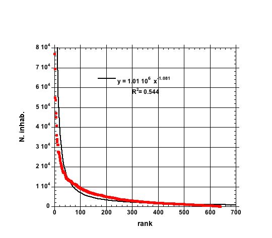
Figure 7: Classical axes display of the rank-size (number of inhabitants in the 639 (637 + 2; see text) Saints generating Italian hagiotoponyms) ranked in decreasing order of the number of inhabitants. A simple power law fit is indicated. Visually, this plot looks like displaying a smoothly decaying data, but the regression coefficient $R^{2}$ is pretty low; alas, as ”better” seen in Fig. 8, it is not possible to find a ”nicely simple” fit.

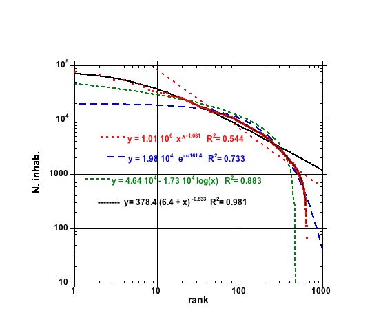
Figure 8: Log-log display of the Number of inhabitants in the 639 (637 + 2; see text) Saints generating Italian hagiotoponyms, - cities ranked in decreasing order of the number of inhabitants; four simple law fits are shown with their corresponding regression coefficient. Visually, from the data scattering, it cannot be expected that a simple empirical law can be found. Indeed, four simple laws are indicated as not giving a nice regression coefficient.
Note that these trial fits with simple empirical laws for the ”all Saints” case, i.e. Fig. 7 and Fig. 8, are not nice enough to suggest a decomposition between males and females.
It is also worth to note that from Fig. 8 it is confirmed that even if regularities of power-law type does not apply for an entire set of data, such regularity may exist for qualified subclusters. This is precisely the case of the hagiotoponym Italian cities, for which four ”regimes” seem to emerge. One is for the 7 or 8 most frequent (in population number) names. The next regime contains about 30 names, and the next one about 50. The final regime contains about 100 names. The first and third regimes have approximately the same power law exponent.

Figure 10: Histogram of the number of cities having a number of inhabitants in some range. Big cities are emphasized, pointing to the presence of outliers.

Figure 11: Log-log plot of the number of inhabitants vs. rank. $K$ represents the 8092 cities, while $C$ is the set of the upper 8092-80 cities, thus removing 80 outliers. It seems that the Lav3 function (green) fits the $C$ data very well; in contrast the fit for the 8092 is not so good.

Figure 12: Also in this case, $K$ represents the 8092 cities, while $C$ is the set of the upper 8092-80 cities, thus removing 80 outliers. As in Fig. 12, one barely sees that the Lav3 function (green) fits the $C$ data very well; in contrast the fit for the 8092 is not satisfactory.

Figure 13: Blow up of the low rank of 8092 cities, Lavalette 3-parameters function. One can see some twisting effect of the function due to the low rank outliers.

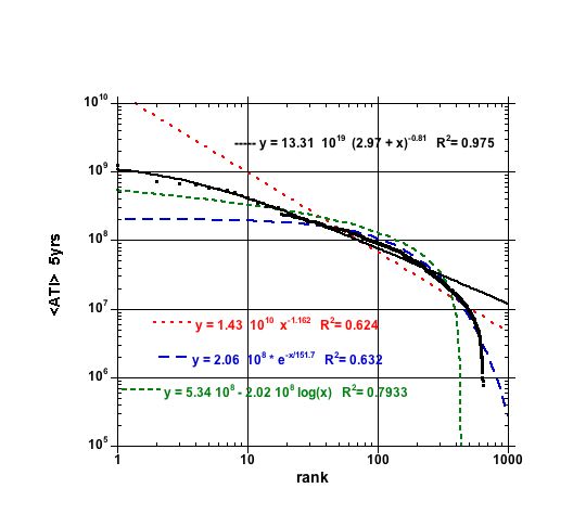
Figure 14: Log-log display of the the average ATI over 5 years for the 639 (637 + 2; see text) Saints generating Italian hagiotoponyms, - cities ranked in decreasing order of the ATI; four simple law fits are shown with their corresponding regression coefficient: power, exponential, log-, and BZM, Eq.(4.4).
Since these trial fits with simple empirical laws in the ”all Italian Saints” case, are not convincing enough to represent the data, they suggest to pursue further a data decomposition between males and females.

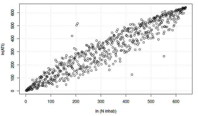
Figure 19: Log-log display of the scatter plot of ranks for the averaged over 5 years ATI and the Number of inhabitants for the 639 Saints generating Italian hagiotoponyms.

References

- [1] Adamic, L.A., (2005). Zipf, Power-laws, and Pareto - a ranking tutorial, .
- [2] Ausloos, M., (2013). A scientometrics law about co-authors and their ranking The co-author core, Scientometrics 95, 895-909.
- [3] Ausloos, M., (2014a). Toward fits to scaling-like data, but with inflection points & generalized Lavalette function, Journal of Applied Quantitative Methods 9, 1-21.
- [4] Ausloos, M., (2014b) Two-exponent Lavalette function. A generalization for the case of adherents to a religious movement, Phys. Rev. E 89, 062803.
- [5] Bradley, T., Essential Statistics for Economics, Business and Management, J. Wiley, Chicheter, 2007.
- [6] Bosker, M., Brakman, S., Garretsen, H., Schramm, M., (2008). A century of shocks: the evolution of the German city size distribution 1925-1999, Regional Science and Urban Economics 38(4), 330-347.
- [7] Caltabiano, M., Dalla Zuanna, G., Rosina, A., (2006). Interdependence between sexual debut and church attendance in Italy, Demographic Research 14(19), 453-484.
- [8] Cerqueti, R., Ausloos, M., (2015). Evidence of Economic Regularities and Disparities of Italian Regions From Aggregated Tax Income Size Data. Physica A: Statistical Mechanics and its Applications 421(1), 187-207.
- [9] Chen, Y., (2012). The rank-size scaling law and entropy-maximizing principle, Physica A 391, 767-778.
- [10] Clauset, A., Shalizi, A.C.C., Newman, M.E.J., (2009). Power-law distributions in empirical data, SIAM Rev. 51, 661-703.
- [11] Connor, P., Koenig, M., (2015). Explaining the Muslim employment gap in Western Europe: Individual-level effects and ethno-religious penalties ?. Social Science Research 49, 191-201.
- [12] Connor, P., (2011). Religion as resource: Religion and immigrant economic incorporation. Social Science Research 40(5), 1350-1361.
- [13] Cordoba, J.-C., (2008). On the distribution of city sizes, Journal of Urban Economics 63(1), 177-197.
- [14] Dennett, D.C., Breaking the Spell: Religion as a Natural Phenomenon, Penguin Group, (2006).
- [15] Dubuisson, D., The Western Construction of Religion: Myths, Knowledge, and Ideology Johns Hopkins Univ. Press, Baltimore (2003).
- [16] Durkheim, E., Les Formes élémentaires de la vie religieuse ; transl: The Elementary Forms of Religious Life (1912). Les Presses universitaires de France, Paris (1968).
- [17] Egghe, L., Waltman, L., (2011). Relations between the shape of a size-frequency distribution and the shape of a rank-frequency distribution, Information Processing and Management 47, 238-245.
- [18] Eliade, M., A History of Religious Ideas, vol. I, From the Stone Age to the Eleusinian Mysteries, Chicago, IL: University of Chicago Press (1978).
- [19] Ellison, C.G., Sherkat, D.E., (1995). Is sociology the core discipline for the scientific study of religion?, Social Forces 73, 1255-1266.
- [20] Fairthorne, R.A. (1969). Empirical hyperbolic distributions (Bradford-Zipf-Mandelbrot) for bibliometric description and prediction, Journal of Documentation 25, 319-343.
- [21] Farmer, D.H., The Oxford dictionary of Saints, Cambridge Univ Press (1987).
- [22] Gabaix, X. (1999). Zipf’s law for cities: An explanation, The Quarterly Journal of Economics 114, 739-767.
- [23] Garmestani, A.S., Allen, C.R., Gallagher, C.M., (2008). Power laws, discontinuities and regional city size distributions, Journal of Economic Behavior and Organization 68, 209-216.
- [24] Gibrat, R. (1957). On economic inequalities, International Economic Papers 7, 53-70.
- [25] Giesen, K., Sudekum, J., (2011). Zipf law for cities in the regions and the country, Journal of Economic Geography 11(4), 667-686.
- [26] Goldstein, M.L., Morris, S.A., Yen, G.G. (2004). Problems with Fitting to the Power-Law Distribution, The European Physical Journal B-Condensed Matter and Complex Systems 41, 255–258.
- [27] Herzel, H., Schmitt, A.O., Ebeling, W., (1994). Finite Sample Effects in Sequence Analysis, Chaos, Solitons & Fractals 4, 97-113.
- [28] Hill, B., (1974). The Rank-Frequency Form of Zipf’s Law, J. Am. Stat. Assoc. 69, 1017-1026.
- [29] Iannaccone, L.R., (1991). The consequences of religious market structure: Adam Smith and the economics of religion, Rationality and Society 3, 156-177.
- [30] Iannaccone, L.R., (1998). An introduction to the economics of religion, Journal of Economic Literature 36, 1465-1496.
- [31] Kendall, M. (1938). A New Measure of Rank Correlation, Biometrika 30(1- 2), 81-89.
- [32] Kim, J., (2007). Pilgrimage and Towns in Medieval Christianity, The 6th Japanese-Korean Symposium on Medieval History of Europe, Keio University, Japan.
- [33] Krugman, P., (1995). Development, Geography, and Economic Theory, The MIT Press, Cambridge, MA.
- [34] Laherrère, J., Sornette, D., (1998). Stretched exponential distributions in nature and economy: fat tails with characteristic scales, European Physical Journal B 2, 525-539.
- [35] Lavalette, D., (1966). Facteur d’impact: impartialité ou impuissance?, Internal Report, INSERM U350, Institut Curie, France.
- [36] Lehrer, E.L., (1995). The effects of religion on the labor supply of married women, Social Science Research 24, 281-301.
- [37] Lehrer, E.L., (1999). Religion as a Determinant of Educational Attainment: An Economic Perspective. Social Science Research 28, 358-379.
- [38] Levenberg, K. (1944). A method for the solution of certain problems in least squares, Quart. Appl. Math. 2, 164-168.
- [39] Lin, S., (2010). Rank aggregation methods, WIREs Computational Statistics 2, 555-570.
- [40] Lourakis, M.I.A. (2011). A Brief Description of the Levenberg-Marquardt Algorithm Implemented by levmar, Foundation of Research and Technology 4, 1-6.
- [41] Mansilla, R., Köppen, E.,Cocho, G., Miramontes, P., (2007). On the behavior of journal impact factor rank-order distribution, Journal of Informetrics 1, 155-160.
- [42] Marquardt, D.W. (1963). An Algorithm for Least-Squares Estimation of Nonlinear Parameters, Journal of the Society for Industrial and Applied Mathematics 11(2), 431-441.
- [43] Martínez-Mekler, G., Martínez, R.A., del Río, M.B., Mansilla, R., Miramontes, P., Cocho, G., (2009). Universality of rank-ordering distributions in the arts and sciences, PLoS ONE 4(3), e4791.
- [44] McKean, J.W., Terpstra J.T., Kloke, J.D., (2009). Computational rank-based statistics, WIREs Computational Statistics 2, 132-140.
- [45] Montroll, E.W., Shlesinger, M.F., (1983). Maximum entropy formalism, fractals, scaling phenomena, and 1/f noise: a tale of tails, J. Stat. Phys. 32, 209-230.
- [46] Morris, C.H., The Concept of Territory in the late Anglo-Saxon and Early Medieval Cult of Saints in England, Master of Philosophy thesis submitted to The University of Birmingham, November 2009.
- [47] Naumis, G.G., Cocho, G., (2008). Tail universalities in rank distributions as an algebraic problem: The beta-like function, Physica A 387, 84-96
- [48] Pareto, V., Cours d’Economie Politique, Geneva, Switzerland: Droz, 1896.
- [49] Popescu, I., Ganciu, M., Penache, M.C., Penache, D., (1997). On the Lavalette ranking law, Romanian Reports in Physics 49, 3-27.
- [50] Popescu, I., (2003). On a Zipf’s Law Extension to Impact Factors, Glottometrics 6, 83-93.
- [51] Rawlings, J.O., Pantula, S.G., Dickey, D.A., Applied regression Analysis - A Research Tool, (SpringerVerlag, New York INC. New York, NY, USA, 1998) pp. 371-372.
- [52] Reading, H.F. Dictionary of the social sciences, Atlantic Publishers Dist. (1996).
- [53] Rose, C., Murray, D., Smith, D., Mathematical Statistics with Mathematica, Springer, New York, 2002, p. 107.
- [54] Shannon, C., (1948). A mathematical theory of communication, Bell Systems Tech. 27, 379-423.
- [55] Soo, K.T., (2007). Zipf law and urban growth in Malaysia, Urban Studies 44(1), 1-14.
- [56] Stark, R., (1996). Why Religious Movements Succeed or Fail: A Revised General Model, J. Contemp. Relig. 11, 133-146.
- [57] Stark, J.R., Bainbridge, W.S., (1979). Of Churches, Sects, and Cults: Preliminary Concepts for a Theory of Religious Movements. J. Sci. Stud. Relig. 18, 117-133.
- [58] Vining, D.R. Jr., (1977). The rank-size rule in the absence of growth, Journal of Urban Economics 4, 15-29.
- [59] Vitanov, N.K., Ausloos, M., (2015). Test of two hypotheses about the sizes of the populations in a system of cities, Journal of Applied Statistics (in press).
- [60] Vitanov, N.K., Dimitrov, Z.I., (2014). Bulgarian cities and the New Economic Geography, Vanio Nedkov, Sofia.
- [61] Voloshynovska, I.A., (2011). Characteristic Features of Rank-Probability Word Distribution in Scientific and Belletristic Literature, Journal of Quantitative Linguistics 18, 274-289.
- [62] Waters, M., Heath, W.C., Watson, J., (1995). A positive model of the determination of religious affiliation, Social Science Quarterly 76(1), 105-123.
- [63] Webb, D. Patrons and Defenders: The Saints in the Italian City-States, Tauris Academic Studies (1996).
- [64] Wessa, P., (2012). Kendall Rank Correlation (v1.0.11), Free Statistics Software (v1.1.23-r7), Office for Research Development and Education, .
- [65] Wieder, T., (2009). The Number of Certain Rankings and Hierarchies Formed from Labeled or Unlabeled, Applied Mathematical Sciences 3(55), 2707 - 2724.
- [66] Wolfe, D.A., (2009). Rank methods, WIREs Computational Statistics 2, 342-347
- [67] Wolfe, D.A., (2010). Ranked set sampling, WIREs Computational Statistics 2, 460-466.
- [68] Yeatman, S.E., Trinitapoli, J., (2008). Beyond denomination: The relationship between religion and family planning in rural Malawi, Demographic Research 19(55), 1851-1882.
- [69] Zhang, L., (2008). Religious affiliation, religiosity, and male and female fertility , Demographic Research 18(8), 233-262.
- [70] Zipf, G.K., Human Behavior and the Principle of Least Effort : An Introduction to Human Ecology, Cambridge, Mass.: Addison Wesley (1949).