Geometric pumping in autophoretic channels

Abstract

Many microfluidic devices use macroscopic pressure differentials to overcome viscous friction and generate flows in microchannels. In this work, we investigate how the chemical and geometric properties of the channel walls can drive a net flow by exploiting the autophoretic slip flows induced along active walls by local concentration gradients of a solute species. We show that chemical patterning of the wall is not required to generate and control a net flux within the channel, rather channel geometry alone is sufficient. Using numerical simulations, we determine how geometric characteristics of the wall influence channel flow rate, and confirm our results analytically in the asymptotic limit of lubrication theory.

I Introduction

Controlled flow manipulation at the micro- or nano-scale is at the heart of recent developments in microfluidics, including many applications in the field of biological analysis and screening (Whitesides, 2006). Generating and controlling a flow within the confined environment of a microfluidic channel requires an external forcing to overcome the viscous stress on the walls. In synthetic micro and nanofluidic systems, this is usually achieved either mechanically, by applying a pressure difference between the inlet and outlet of the domain, or through electrokinetics /electroosmosis, where the flow results from an externally-imposed electric field within the channel (Squires and Quake, 2005; Sia and Whitesides, 2003; Ajdari, 1995, 2000).

However, many biological systems rely on stresses localized at boundaries in order to drive flow, rather than on a global macroscopic forcing. For example, microscopic cilia on the lung epithelium induce a directional flow of mucus through their coordinated beating, acting as a pump (Sleigh et al., 1988). Similar microscale flow forcing at the wall also plays an essential role in the early stages of embryo development (Hirokawa et al., 2009) or in the reproduction of mammals, where cilia-driven flow is responsible for the migration of the ovum down the female reproductive tract (Halbert et al., 1976).

In a dual process, cilia-driven flows play an essential role in the self-propulsion of micro-organisms such as Paramecium (Brennen and Winnet, 1977); the flow generated by the beating of cilia anchored on the wall of a moving cell is responsible for its locomotion. For both swimming and pumping, the coordination of neighboring cilia into metachronal wave patterns has been proven essential to achieving maximum flow rate/swimming speed with a minimum energetic cost (Gueron and Levit-Gurevich, 1999; Michelin and Lauga, 2010; Osterman and Vilfan, 2011; Hussong et al., 2011; Elgeti and Gompper, 2013).

Several attempts have been made to reproduce ciliary pumping in the lab through the fabrication of artificial actuated cilia (Toonder et al., 2008; Fahrni et al., 2009; Babataheri et al., 2011; Coq et al., 2011). All of them rely, however, on the application of a global electromagnetic forcing field, and generating efficient pumping would require the application of phase-shifted forcing on neighboring cilia (Khaderi et al., 2011, 2012). This constraint, as well as the manufacturing process of microscopic cilia, poses important challenges to miniaturization.

Phoretic mechanisms, namely the ability to generate fluid motion near a boundary under the effect of an external field gradient, represent an alternative route for both pumping and swimming systems that require no moving parts. These mechanisms arise from the interaction of rigid boundaries with neutral or ionic solute species in their immediate environment, and are known to generate the migration of passive particles in external gradients (Anderson, 1989). Phoretic motion has recently received renewed attention in the context of artificial self-propelled systems. Such artificial swimmers generate the field gradients required for propulsion themselves, for example through chemical reactions catalyzed at their surface, and thus do not rely on any external forcing to achieve propulsion (Paxton et al., 2004; Howse et al., 2007; Golestanian et al., 2007; Palacci et al., 2013). These systems combine two properties: (i) an activity, i.e. the ability to release/consume solute species or thermal energy at their surface, and (ii) a phoretic mobility, i.e. the ability to create a slip velocity at the boundary from a local tangential gradient of solute concentration (diffusiophoresis), temperature (thermophoresis) or electric potential (electrophoresis). Recently, autophoretic systems have also been considered for generating micro-rotors that rotate without the application of external torques (Yang and Ripoll, 2014; Yang et al., 2015).

In order to generate the surface gradients necessary to their self-propulsion, autophoretic particles must break spatial symmetry. A similar requirement exists for autophoretic pumps. This symmetry-breaking may be achieved for self-propelled particles following three main routes: (i) chemical asymmetry, i.e. patterning the particle surface with active and passive sites (e.g. Janus particles) (Golestanian et al., 2007; Howse et al., 2007; Theurkauff et al., 2012), (ii) spontaneous symmetry-breaking resulting from the advection of the field responsible for the phoretic response by the flow itself (Michelin et al., 2013; Izri et al., 2014) and (iii) geometric asymmetry (Shklyaev et al., 2014; Michelin and Lauga, 2015).

In this work, we use a combination of theoretical analysis and numerical simulations to investigate whether, and how, autophoretic mechanisms and geometric asymmetry can generate a net flow in a microfluidic channel without imposing any external mechanical forcing, electromagnetic forcing or chemical patterning. For simplicity we focus on the specific case of diffusiophoresis, where slip velocities are generated at the wall from tangential gradients in the concentration of a solute released from one of the channel walls into the fluid. Because of the similarity between the different phoretic mechanisms, it is expected that the results of the present contribution may easily be generalized to thermo- or electrophoretic systems. Specifically, we follow the classical continuum framework of self-diffusiophoresis (Golestanian et al., 2007; Jülicher and Prost, 2009; Sabass and Seifert, 2012; Michelin and Lauga, 2014), and consider how a left-right asymmetry in the wall shape can generate a net flow within the channel which hence acts as a microfluidic pump.

The paper is organized as follows. Section II summarizes this continuum framework for the case of the flow within an asymmetric channel, and presents the numerical methods used in this work. Section III shows how the wall geometric characteristics determine the net flow within the channel. The results are then confirmed analytically in Sec. IV using lubrication theory in the long-wavelength limit, and conclusions and perspectives are presented in Sec. V.

II Problem formulation

II.1 Diffusiophoretic channel

We consider a two-dimensional channel of mean height $H$, bounded by a flat bottom boundary ($y=0$) and a top wall with a periodic non-flat profile, $y=h(x)$ (see illustration in Figure 1). In the channel gap, filled with a Newtonian fluid of dynamic viscosity $\mu$ and density $\rho$, a solute species of local concentration $C(\mathbf{x})$ with molecular diffusivity $D$ is present and interacts with the channel walls through a short range potential. When the typical thickness of this interaction region is much smaller than the other length scales of the problem (namely the channel gap and the wavelength), the interaction of the wall with a local solute gradient generates an effective slip velocity at the wall (Anderson, 1989; Michelin and Lauga, 2014)

$$\mathbf{u}_{\textrm{slip}}=M\boldsymbol{\nabla}_{\parallel}C,$$ (1)

where $\boldsymbol{\nabla}_{\parallel}=(\mathbf{1}-\mathbf{n}\mathbf{n})\cdot\boldsymbol{\nabla}$ is the tangential component of the gradient to the surface of local normal $\mathbf{n}$ and $M$, the phoretic mobility, is a property of the solute-wall interaction which may be positive or negative depending on the repulsive or attractive nature of that interaction (Anderson, 1989). The chemical properties of the channel walls are also characterized by a chemical activity, i.e. the ability to create or consume the solute species. Here we consider a simple fixed-flux model, for which the activity of the wall is given by a fixed flux of solute per unit area $A$, counted positively (resp. negatively) when solute is released (resp. absorbed)

$$D\,\mathbf{n}\cdot\boldsymbol{\nabla}C=-A.$$ (2)

In the case of self-diffusiophoretic propulsion, locomotion is often achieved through inhomogeneity in the chemical treatment of the particle (Paxton et al., 2004; Howse et al., 2007; Golestanian et al., 2007). Recent work has shown that geometric asymmetry of chemically-homogeneous particle alone is in fact sufficient to ensure locomotion (Shklyaev et al., 2014; Michelin and Lauga, 2015). Here we investigate a similar question, namely the possibility of obtaining a net flow from chemically-homogeneous channel walls using shape asymmetry. We thus assume that the top corrugated wall has homogeneous mobility $M$ and activity $A$. To ensure the existence of a steady state solution, the concentration of the solute on the bottom wall is assumed to be fixed ($C=C_{0}$). Consequently, the fluid velocity on that wall satisfies the no-slip boundary condition. By studying the relative concentration of solute to that on the bottom wall, we can assume without loss of generality that $C_{0}=0$.

The phoretic slip velocity generated at the top wall by the wall-solute interaction drives a flow within the channel. When viscous effects dominate inertia (namely, when the Reynolds number $\mbox{Re}=\rho\mathcal{U}H/\mu$ is small, with $\mathcal{U}={\color[rgb]{0,0,0}|AM|}/D$ the typical phoretic velocity), the flow satisfies the incompressible Stokes equations

$$\mu\nabla^{2}\mathbf{u}=\boldsymbol{\nabla}p,\qquad\boldsymbol{\nabla}\cdot\mathbf{u}=0,$$ (3)

for the velocity and pressure fields, $\mathbf{u}$ and $p$ respectively. Solute molecules diffuse within the channel, and in general can also be advected by the phoretic flows. However, when diffusive effects dominate (i.e. when the Péclet number, $\mbox{Pe}=\mathcal{U}H/D$, is small), the solute dynamics is completely decoupled from the flow, and the solute concentration satisfies Laplace’s equation

$$\nabla^{2}C=0.$$ (4)

Equations (3)–(4), together with the boundary conditions Eqs. (1)–(2) applied at the top wall and the inert boundary conditions $C=0$ and $\mathbf{u}=\mathbf{0}$ at the bottom wall, form a closed set of equations that can be solved successively for the solute concentration $C$ and velocity field ${\color[rgb]{0,0,0}\mathbf{u}=(u,v)}$. From these results, the net flow rate within the channel, $Q$, can be computed as

$$Q=\int_{0}^{h(x)}u(x,y)\mathrm{d}y,$$ (5)

which is independent of $x$ because the flow is incompressible.

II.2 Asymmetric channel

The shape of the channel is a periodic function of $x$ characterized by a wavenumber $k=2\pi/L$. A sinusoidal wall will generate a perfectly left-right-symmetric concentration distribution and flow pattern, leading to no net flow along the channel. In the following, we focus on a subset of asymmetric wall shapes, essentially smoothed ratchets, that are formally obtained by mathematically shearing the symmetric sinusoidal profile. The top wall is described in parametric form by

$$x(s)=s-\frac{\gamma}{k}\sin ks,\qquad y(s)=H+a\sin ks,$$ (6)

the non-dimensional asymmetry parameter, $\gamma$, determines the asymmetry of the profile, and $H$ and $a$ are the mean channel width and the amplitude of the width fluctuations, respectively (see Figure 1).

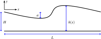
Figure 1: Asymmetric phoretic channel. The top wall is characterized by constant chemical activity $A$ and mobility $M$. The bottom wall maintains a fixed concentration and thus flow satisfies no-slip there. The example shown here corresponds to $\gamma=\pi/4$, $a/H=1/2$ and $L/H=2\pi$ with the asymmetric shape of the wall given in Eq. (6).

Hereafter, the problem is non-dimensionalized using $1/k$ as characteristic length, $\mathcal{U}$ as characteristic velocity, and ${\color[rgb]{0,0,0}|A|}/Dk$ as characteristic concentration fluctuation. While $A$ and $M$ are both signed quantities, after nondimensionalisation we focus on the case $A=M=1$; changing the sign of either $A$ or $M$ simply reverses the slip velocity forcing and flow rate without changing its magnitude. The problem is now completely specified by three geometrical quantities, namely the non-dimensional mean gap, $H^{*}=kH$, the corrugation amplitude, $a^{*}=ka$, and the asymmetry parameter, $\gamma$.

II.3 Numerical method

Equation (3) for the solute concentration and Eq. (4) for the flow and pressure fields are solved numerically using a boundary integral approach with periodic Green’s functions.

We denote $\Omega$ the fluid domain in a period of the channel gap, $\partial\Omega$ its lower and upper boundaries (the inert and active walls), and $\mathbf{n}$ the unit normal vector pointing into the fluid domain. The two-dimensional periodic Green’s function for Laplace’s equation, Eq. (4), is given by

$$\Phi(x,y;\xi,\eta)= \ \frac{1}{4\pi}\sum_{{\color[rgb]{0,0,0}n=}-\infty}^{\infty}\ln\left[(x-\xi+2n\pi)^{2}+(y-\eta)^{2}\right]$$

$$= \ \frac{1}{4\pi}\ln[2(\cosh(y-\eta)-\cos(x-\xi))].$$ (7)

Assuming that the channel walls are smooth, the concentration at a point $(x,y)$ on one of the walls can then be computed using the boundary integral formulation (Banerjee and Butterfield, 1981)

$$\frac{1}{2}C(x,y)= \int_{\partial\Omega}\left[C(\xi,\eta)\frac{\partial}{\partial n}(\Phi(x,y;\xi,\eta))\right.$$

$$-\left.\Phi(x,y;\xi,\eta)\frac{\partial}{\partial n}(C(\xi,\eta))\right]\mathrm{d}s(\xi,\eta).$$ (8)

The upper and lower boundaries of the domain are discretized into $200$ straight-line segments, and $C$ and $\mathrm{d}C/\mathrm{d}n$ are assumed constant over each element. For elements on the bottom (resp. top) boundary, $C=0$ (resp. $\mathrm{d}C/\mathrm{d}n=-1$) is enforced at the midpoint of each segment. This reduces the boundary integral equation (7) to a dense matrix system for the solution vector containing the unknown $\mathrm{d}C/\mathrm{d}n$ on the lower boundary and $C$ on the upper boundary. The free-space (i.e. singular) component of the Green’s function is isolated and integrated analytically, and all non-singular element integrals are computed with a $16$-point Gaussian quadrature. In order to compute the fluid flow and flow rate in the channel, only the boundary concentration of solute (and not its bulk distribution) is needed, which makes the boundary element method particularly suitable for this problem. The numerical code was validated against analytical solutions for diffusion in a channel with nontrivial boundary conditions and domain geometry, achieving a relative error of at worst $0.004\%$.

For Stokes flow, the dimensionless boundary integral equation for boundary force density, $\mathbf{f}$, is given by

$$u_{j}(\mathbf{x})=\frac{1}{2\pi} \int_{{\color[rgb]{0,0,0}\partial\Omega}}[S_{ij}(\mathbf{x}-\boldsymbol{\xi})f_{i}(\boldsymbol{\xi})$$

$$-T_{ijk}(\mathbf{x}-\boldsymbol{\xi})u_{i}(\boldsymbol{\xi})n_{k}(\boldsymbol{\xi})]\mathrm{d}s(\boldsymbol{\xi}).$$ (9)

For $\hat{\mathbf{x}}=\mathbf{x}-\boldsymbol{\xi}$ and $r=|\hat{\mathbf{x}}|$, the two-dimensional, $2\pi$-periodic Green’s functions for Stokes flow are

$$\mathbf{S}=\sum_{n=-\infty}^{\infty}\mathbf{I}\ln r_{n}-\frac{\hat{\mathbf{x}}_{n}\hat{\mathbf{x}}_{n}}{r_{n}^{2}},\quad\mathbf{T}=\sum_{n=-\infty}^{\infty}4\frac{\hat{\mathbf{x}}_{n}\hat{\mathbf{x}}_{n}\hat{\mathbf{x}}_{n}}{r_{n}^{4}},$$ (10)

where $\hat{\mathbf{x}}_{n}=\left(x-\xi+2n\pi,y-\eta\right)$. These functions may be expressed in the closed form

$$\begin{aligned} S_{xx}&=K+\hat{y}\partial_{\hat{y}}K-1,\\ S_{yy}&=K-\hat{y}\partial_{\hat{y}}K,\\ S_{xy}&=-\hat{y}\partial_{\hat{x}}K=S_{yx},\\ T_{xxx}&=2\partial_{\hat{x}}(2K+\hat{y}\partial_{\hat{y}}K),\\ \end{aligned}\qquad\begin{aligned} T_{xxy}&=2\partial_{\hat{y}}(\hat{y}\partial_{\hat{y}}K),\\ T_{xyy}&=-2\hat{y}\partial_{\hat{x}\hat{y}}K,\\ T_{yyy}&=2(\partial_{\hat{y}}K-\hat{y}\partial_{\hat{y}\hat{y}}K),\\ T_{ijk}&=T_{kij}=T_{jki},\end{aligned}$$ (11)

for $K=\frac{1}{2}\ln\left[2\cosh(\hat{y})-2\cos(\hat{x})\right]$. The computational procedure for discretizing the domain boundary is identical to that used for the diffusion equation (7). Constant force elements are assumed, singular integrals have the singularity removed and computed analytically, and non-singular integrals are computed with 16- point Gaussian quadrature.The implementation is based upon the authors’ previously published work on the optimal swimming of a sheet (Montenegro-Johnson and Lauga, 2014), with the addition of Tikhonov regularisation to improve matrix conditioning.

III Results

III.1 The role of asymmetry

When inertia and solute advection are negligible, the Laplace problem for the solute concentration is linear and decouples from the Stokes flow problem, which is also linear. Breaking the left-right symmetry is thus required in order to create a net flow within the channel, in the same way that symmetry breaking is required to achieve self-propulsion of autophoretic particles. If the chemical properties of the walls are homogeneous, this asymmetry can only arise from geometry and therefore, purely symmetric profiles such as sinusoidal upper-wall shapes will yield zero net flux.

In order to analyze the effect of asymmetry, we first investigate the effect of the asymmetry parameter, $\gamma$, on the flow rate. The numerical results are shown in Figure 2. At $\gamma=0$, we recover zero-net flux, as expected. For asymmetric shapes, we obtain that the flow rate within the channel increases monotonically with $\gamma$.

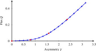
Figure 2: Dependence of the net flow rate through the channel, $Q$, with the left-right asymmetry of the top wall, $\gamma$, in the cases $a/H=1/2$, $L/H=2\pi$ and $0\leq\gamma\leq\pi$. The four red dots correspond to the different panels illustrated in Figure LABEL:fig:streamlines.

To gain insight into the origin of this flow rate, we illustrate in Figure LABEL:fig:streamlines the dependence of the solute concentration distribution and streamlines with $\gamma$. For a strictly symmetric profile, $\gamma=0$, a flow is induced in the channel but one with no net flux. Indeed, a vertical solute concentration gradient is created between the two walls due to the fixed-flux emission of solute at the upper wall and the constant concentration imposed at the lower wall, where the solute is consumed. The upper wall is not horizontal, and regions of the upper wall located the furthest from the bottom wall are exposed to higher concentration than regions corresponding to the narrowest channel width. This implies the existence of tangential solute gradients along the wall and, hence, of a slip velocity that drives a flow within the channel. Due to the symmetry of the channel, the flow organizes into two counter-rotating flow cells leading to zero fluid transport across the channel. For positive activity and mobility of the upper wall, the flow is directed away from the active wall (i.e. downward) in the regions where the channel width is greatest, while it is directed toward the active wall (i.e. upward) in the narrowest regions (Figure LABEL:fig:streamlinesa).

When $\gamma\neq 0$, asymmetry is introduced in two ways. The asymmetric upper wall can now be decomposed into a longer backward facing section and a shorter forward-facing section. The solute gradient on the former is weaker than on the latter, leading to a stronger left-to-right slip flow along the forward facing section. Additionally, wall asymmetry increases confinement in the trough along the upper wall leading to higher solute concentration (the rate of production of solute per unit surface is fixed). This asymmetry between the wall sections driving the flow within the channel generates a shape and intensity asymmetry between the two recirculation regions, and a traversing streamtube appears (marked by dark red streamlines in Figure LABEL:fig:streamlines). This streamtube corresponds to flow regions that do not recirculate, but are transported along the channel, being “pumped” by the phoretic mechanism. This tube follows a pattern along the channel similar to that of a conveyor belt driven between the two recirculating regions forced by the slip flow on the wall. Along the shorter forward-facing section of the upper wall, it is driven by the stronger slip flow that dictates the direction of the net flow in this case. The tube then separates from the wall where the slip velocity changes sign, and circumnavigates around the counter-rotating flow cell driven by the longer wall section.

As $\gamma$ is increased beyond $\gamma\geq 1$, the slope of the shorter flow-driving wall changes sign, leading to a “folded” geometry that promotes large confinement effects on the solute concentration distribution (see the difference in color scales in Figure LABEL:fig:streamlines). This, in turn, enhances the phoretic slip and net flow rate. For strong asymmetry, the traversing streamtube is mostly rectilinear and away from the active wall, except in a narrowing region where it circles around the smaller recirculation region and is driven by the phoretic slip within the trough on the boundary.

This process does not appear to saturate when $\gamma\gg 1$ for fixed amplitude $a$. In this limit, the flow domain can be decomposed into two regions: a complex, thin region corresponding to long and thin folds in the wall shape where very large concentration gradients are established by confinement, and an outer region where a net unidirectional flow is forced within the channel. Beyond obvious practical considerations regarding the manufacturing of such geometries, the assumptions of the current model would potentially break down when the asymmetry parameter $\gamma$ becomes too large, as the phoretic flow become sufficiently intense for advection to be non-negligible ($\mbox{Pe}\neq 0$). Furthermore, when local concentrations become too large, it is likely that the model of fixed-flux release would be impacted, and more detailed reaction kinetics may be required.

III.2 Effect of the pattern amplitude on the flow rate

The flow within the channel is effectively driven by the upper wall, while the no-slip condition on the lower inert wall tends to limit the fluid motion. As a consequence, it is expected that when the channel gap in the narrowest region becomes small ($a\approx H$), the net flow rate should be small, as the flow viscosity will offer maximum resistance there. However, the corrugation amplitude is an essential element to the pumping performance of the device as it determines the gradient along the upper wall between the peak and troughs, and therefore the intensity of the two recirculating regions driving the flow. When $a\ll H$, it is therefore also expected that the flow rate will become negligible. This intuition is confirmed by our numerical results in the case of weak asymmetry ($\gamma\leq 1$, unfolded geometry, see Figure LABEL:fig:amplitudea) for which the net flow rate within the channel displays a maximum at intermediate amplitude and decreases to zero in both limits $a\ll H$ and $a\approx H$. In this case, the limit $a\ll H$ corresponds to a flat upper wall.

The behavior of the system is however quite different when the upper wall is folded ($\gamma\geq 1$, strong asymmetry, see Figure LABEL:fig:amplitudeb). In this case, the limit $a\ll H$ is not limiting to a flat wall, but to a surface with infinitely thin and almost horizontal folds. Within these folds, confinement creates very large solute concentrations and concentration gradients. As noted in the previous section, this limit is the singular case of a flat wall forced periodically by infinitely large slip velocities in infinitely thin regions. As a consequence, the net flow rate does not decrease to zero for small amplitude, marking a stark difference between the folded and unfolded geometries.

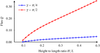
Figure 5: Net flow rate through the channel, $Q$, as a function of the channel height $H/L$ for unfolded $\gamma=\pi/4$ and folded $\gamma=\pi/2$ channels with fixed relative amplitude, $a/L=0.08$.

III.3 Role of the channel width

We finally turn to the influence of the third geometric characteristic of the channel, namely its mean width-to-length ratio. The limit of small minimum width ($a\approx H$) was already discussed in the previous section and the flow rate within the channel vanishes in that limit due to the diverging hydrodynamic resistance of the channel. When $H$ is large compared to both $a$ and $L$, the relative concentration distribution along the top wall is not influence by the location of the passive wall so the tangential concentration gradients and slip velocity become independent of $H$. As a result the net flow rate through the channel varies linearly with the channel height as for a classical Couette (shear) flow. This is confirmed by our numerical results shown in Figure 5.

IV Long-wavelength prediction

When the local height of the channel is small in comparison to the typical longitudinal length of the topography, i.e. $|h^{\prime}(x)|\ll 1$, the problem can be solved within the framework of lubrication (long-wavelength) theory. Defining $h(x)=\varepsilon f(x)$ with $f(x)=O(1)$ and $\varepsilon{\color[rgb]{0,0,0}=H/L}\ll 1$, the method consists in solving for the concentration and velocity fields as regular series expansions in $\varepsilon$. On the upper wall, the normal unit vector pointing into the fluid is now written

$$\mathbf{n} =\frac{-\mathbf{e}_{y}+h^{\prime}\mathbf{e}_{x}}{\sqrt{1+h^{{}^{\prime}2}}}$$

$$=-\mathbf{e}_{y}+\varepsilon f^{\prime}\mathbf{e}_{x}+\frac{\varepsilon^{2}f^{{}^{\prime}2}}{2}\mathbf{e}_{y}-\frac{\varepsilon^{3}f^{{}^{\prime}3}}{2}\mathbf{e}_{x}+O(\varepsilon^{4}).$$ (12)

Defining a rescaled vertical coordinate $y=\varepsilon Y$, the Laplace and Stokes flow problems are now given by

$$\frac{1}{\varepsilon^{2}}\frac{\partial^{2}C}{\partial Y^{2}}+\frac{\partial^{2}C}{\partial x^{2}} =0,$$ (13a)

$$\frac{1}{\varepsilon^{2}}\frac{\partial^{2}u}{\partial Y^{2}}+\frac{\partial^{2}u}{\partial x^{2}} =\frac{\partial p}{\partial x},$$ (13b)

$$\frac{1}{\varepsilon^{2}}\frac{\partial^{2}v}{\partial Y^{2}}+\frac{\partial^{2}v}{\partial x^{2}} =\frac{1}{\varepsilon}\frac{\partial p}{\partial Y},$$ (13c)

$$\frac{1}{\varepsilon}\frac{\partial v}{\partial Y}+\frac{\partial u}{\partial x} =0,$$ (13d)

and the boundary conditions at $y=\varepsilon f(x)$ become

$$-1 =-\frac{1}{\varepsilon}\frac{\partial C}{\partial Y}+\varepsilon\left(f^{\prime}\frac{\partial C}{\partial x}+\frac{f^{{}^{\prime}2}}{2}\frac{\partial C}{\partial Y}\right)+O(\varepsilon^{3}C),$$ (14a)

$$u =\left(\frac{\partial C}{\partial x}+f^{\prime}\frac{\partial C}{\partial Y}\right)\left(1-\varepsilon^{2}f^{{}^{\prime}2}\right)+O(\varepsilon^{4}C),$$ (14b)

$$v =\varepsilon f^{\prime}\left(\frac{\partial C}{\partial x}+f^{\prime}\frac{\partial C}{\partial Y}\right)+O(\varepsilon^{3}C).$$ (14c)

These, together with the conditions ${\color[rgb]{0,0,0}C}=0$ and $u=v=0$ at ${\color[rgb]{0,0,0}Y}=0$, suggest searching for solutions of the form

$$C(x,{\color[rgb]{0,0,0}Y}) =\varepsilon C_{1}(x,{\color[rgb]{0,0,0}Y})+\varepsilon^{3}C_{3}(x,{\color[rgb]{0,0,0}Y})+O(\varepsilon^{5}),$$ (15a)

$$u(x,{\color[rgb]{0,0,0}Y}) =\varepsilon u_{1}(x,{\color[rgb]{0,0,0}Y})+\varepsilon^{3}u_{3}(x,{\color[rgb]{0,0,0}Y})+O(\varepsilon^{5}),$$ (15b)

$$v(x,{\color[rgb]{0,0,0}Y}) =\varepsilon^{2}v_{2}(x,{\color[rgb]{0,0,0}Y})+O(\varepsilon^{4}),$$ (15c)

$$p(x,{\color[rgb]{0,0,0}Y}) =\varepsilon^{-1}p_{-1}(x,{\color[rgb]{0,0,0}Y})+\varepsilon p_{1}(x,{\color[rgb]{0,0,0}Y})+O(\varepsilon^{3}).$$ (15d)

The flow rate $Q$ is then given by

$$Q=\varepsilon\int_{0}^{f(x)}u(x,Y)\mathrm{d}Y=\varepsilon^{2}Q_{2}+\varepsilon^{4}Q_{4}+O(\varepsilon^{6}),$$ (16)

with

$$Q_{j}=\int_{0}^{f}u_{j-1}(x,Y)\mathrm{d}Y.$$ (17)

The flow is incompressible and steady, therefore $Q$ and $Q_{j}$ do not depend on $x$.

Inserting Eq. (15a) into Eqs. (13a) and (14a) gives at leading order

$$C_{1}(x,Y)=Y.$$ (18)

Eqs. (13b), (14b) and (15b) then provide at $O(\varepsilon)$:

$$u_{1}(x,Y)=\frac{p_{-1}^{\prime}}{2}(Y^{2}-Yf)+\frac{Yf^{\prime}}{f},$$ (19)

with $p_{-1}$ the leading-order pressure distribution which is vertically invariant. The function $p_{-1}(x)$ is periodic, therefore

$$Q_{2}=0\quad\textrm{and}\quad p_{-1}(x)=-6/f.$$ (20)

We see that in the lubrication limit, a velocity field is present at $O(\varepsilon)$, which takes the form of two recirculating regions, but does not give rise to any net flow through the channel at this order. After substitution and application of the continuity equation, we obtain

$$u_{1}(x,Y) =3\left(\frac{f^{\prime}}{f^{2}}\right)Y^{2}-2\left(\frac{f^{\prime}}{f}\right)Y,$$ (21a)

$$v_{2}(x,Y) =\left(\frac{f^{\prime}}{f}\right)^{\prime}Y^{2}-\left(\frac{f^{\prime}}{f^{2}}\right)^{\prime}Y^{3}.$$ (21b)

At next order, the Laplace problem, Eqs. (13a) and (14a), together with Eq. (18), provide

$$C_{3}(x,Y)=\frac{Yf^{{}^{\prime}2}}{2}\cdot$$ (22)

The horizontal Stokes flow problem now yields,

$$u_{3}(x,Y) =2\left[\left(\frac{f^{\prime}}{f}\right)^{\prime\prime}\left(\frac{Y^{3}-Yf^{2}}{3}\right)-\left(\frac{f^{\prime}}{f^{2}}\right)^{\prime\prime}\left(\frac{Y^{4}-Yf^{3}}{4}\right)\right]$$

$$+\frac{\tilde{p}_{1}^{\prime}}{2}(Y^{2}-{\color[rgb]{0,0,0}Y}f)+\left(ff^{\prime}f^{\prime\prime}-\frac{f^{{}^{\prime}3}}{2}\right)\frac{Y}{f},$$ (23)

with $\tilde{p}_{1}(x)$ a function of $x$ only. Integrating the previous equation in $Y$ finally provides the flow rate at $O(\varepsilon^{4})$

$$Q_{4} =2\left[\frac{3f^{5}}{40}\left(\frac{f^{\prime}}{f^{2}}\right)^{\prime\prime}-\frac{f^{4}}{12}\left(\frac{f^{\prime}}{f}\right)^{\prime\prime}\right]-\frac{\tilde{p}^{\prime}_{1}}{12}f^{3}$$

$$+\left(\frac{f^{2}f^{\prime}f^{\prime\prime}}{2}-\frac{ff^{\prime 3}}{4}\right).$$ (24)

Using the periodicity of $\tilde{p}_{1}$, $Q_{4}$ can be computed by dividing the previous equation by $f^{3}$, taking the spatial average in $x$, and integration by parts. The result can be rewritten in terms of the original channel height $h(x)$. At leading order we obtain that the flow through the channel is given by

$$Q=\frac{11}{30}\frac{\left\langle h^{{}^{\prime}3}/h^{2}\right\rangle}{\left\langle 1/h^{3}\right\rangle},$$ (25)

where $\left\langle\cdot\right\rangle$ is the spatial average over a period.

We see two important results: (i) the flow rate is intimately linked to the distribution of local slope along the wall $h^{\prime}(x)$, and (ii) shape asymmetry is essential for the existence of a net flow. Indeed, slip flow along the active wall arises from the orientation of the wall with a component along the leading order solute concentration gradient. A non zero $h^{\prime}(x)$ is therefore sufficient to guarantee the existence of a local flow but not necessarily of a net flow through the channel. This separation of scales is clearly visible in the lubrication expansion: the leading order flow arises from the local channel geometry (i.e. the fact that the wall is not flat and orthogonal to the leading order solute gradient). However, at this order, the net flow is zero because the flows driven by the forward- and backward-facing walls exactly cancel out. A net flux results from an imbalance between these local flows which can only be induced by geometric asymmetry. Left-right symmetric profiles are characterized by an even channel height, $h(x)=h(-x)$. Consequently the function $h^{{}^{\prime}3}/h^{2}$ is odd and thus exactly averages to zero, so that $Q_{4}$ is identically zero (all higher orders are expected to be zero as well).

The result in Eq. (25) is a weighted algebraic spatial average of the slope of the active wall. More precisely, the leading order flow rate through the channel, Eq. (25), is the ratio of two integrals; the numerator is the mean flow forcing due to the asymmetry of the channel, while the denominator is the average hydrodynamic resistance of the channel over a wavelength.

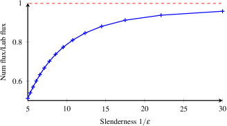
Figure 6: Ratio between the numerical results and the lubrication (long-wavelength) theory predictions for $\gamma=\pi/10$ and $a=H/3$ as a function of an increasing slenderness, $1/\varepsilon$.

This leading-order prediction is compared to the full numerical simulations in Figure 6. For a fixed asymmetry parameter $\gamma$ and relative amplitude $a/H$, several simulations are performed for increasing $L/H$ (note that as $H$ is reduced, $a$ is reduced in the same amount) and the flow rate through the channel is shown to converge for large slenderness to the prediction of the lubrication theory.

Note that the lubrication result, Eq. (25), is valid for any ratio $H/L\ll 1$, regardless of the relative magnitude of the mean channel height $H$ and the perturbation amplitude $a$. In the limit of small wall roughness ($a\ll H$), the hydrodynamic resistance (the denominator in Eq. 25) is independent of $a$ at leading order and simply scales as $1/H^{3}$, while the phoretic forcing (the numerator in Eq. 25) scales as $a^{3}/H^{2}$. As a consequence, $Q$ scales as $a^{3}H$ when $a\ll H$.

In the opposite limit $a\sim H$, using classical asymptotic expansions to compute the leading order contribution to the integrals in Eq. (25) (Bender and Orszag, 1978), one can show that the flow forcing due to the channel’s asymmetry (i.e. the numerator in Eq. 25) remains finite and $O(H)$, but that in contrast the hydrodynamic resistance diverges. More specifically, a standard lubrication calculation leads at leading order to

$$\left\langle\frac{1}{h^{3}}\right\rangle=\frac{3\sqrt{2}}{16H^{1/2}(H-a)^{5/2}}\cdot$$ (26)

As a consequence, $Q\sim H^{3/2}(H-a)^{5/2}$ when $(H-a)\ll H$.

Note that since the limiting factor is then the channel width at the narrowest point, and its impact on the hydrodynamic resistance, it is expected that this scaling in $(H-a)^{5/2}$ should hold true even when $H$ is not small and could be recovered through a new lubrication expansion limited to the narrow-gap region of the channel (Leal, 2007), provided the curvature of the wall in that region remains finite.

V Conclusions

The active research in recent years on autophoretic particles has demonstrated that fuel-based mechanisms represent a promising route to designing self-propelled systems that rely only on chemical reactions and the interaction with the immediate environment to create locomotion. The results presented in this work show that this is also true for the dual problem of pumping flow within a micro-channel, and that geometric asymmetry, rather than chemical patterning of the channel walls, is sufficient to create a net flow. Our results provide insight into the flow dynamics within the channel, and the mechanism leading to the net fluid transport: the breaking of symmetry between two recirculating flow regions driven by wall slip velocity, and the emergence of a conveyor-belt-like flow within the channel.

For simplicity, we focused in this paper on a reduced set of wall shapes with one active wall and the other one passive. The numerical methodology and the long-wavelength theory, Eq. (25), are however valid for any periodic channel geometry in two dimensions. Furthermore, these results were obtained within the simplified framework of a fixed-rate release of solute by the active wall. Previous studies on autophoretic self-propelled particles have shown that the exact reaction kinetics, in particular the dependence of the reaction rate on the local solute concentration, may significantly impact the system dynamics (Ebbens et al., 2012; Michelin and Lauga, 2014). We expect for example the direction of pumping to be impacted by reaction kinetics, although the basic result showing the emergence of a net flow due to geometric asymmetry of the phoretic wall should remain true. Finally, our study focused on the particular case of self-diffusiophoresis. Because of the formal similarities in the equations of the problem, these results can be generalized easily to other phoretic mechanisms such as self-thermophoresis or self-electrophoresis.

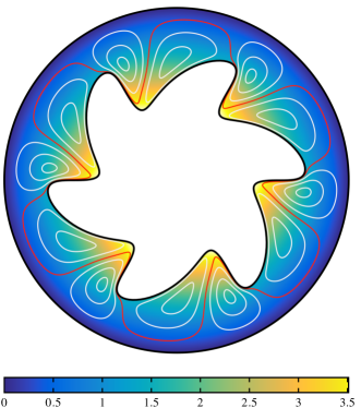
Figure 7: Concentration distribution and flow streamlines within an annular closed-loop channel with a geometrically-asymmetric inner active wall releasing solute with a fixed flux, and a passive circular outer wall with uniform concentration. The recirculating streamlines are shown in white while the traversing streamlines are plotted in red, and correspond to a clockwise-rotating flow.

Looking forward, the results of this work could be generalized to a larger range of geometries, including closed-loop channels for which pressure-driven flows can not easily be achieved. This is shown in Figure 7 where we have adapted our numerical approach to compute the net clockwise flow through a two-dimensional annular channel driven by the geometric asymmetry of the inner active wall.

References

- Whitesides (2006) G. M. Whitesides, Nature, 2006, 442, 368–373.
- Squires and Quake (2005) T. M. Squires and S. R. Quake, Rev. Mod. Phys., 2005, 77, 977–1026.
- Sia and Whitesides (2003) S. K. Sia and G. M. Whitesides, Electrophoresis, 2003, 24, 3563–3576.
- Ajdari (1995) A. Ajdari, Phys. Rev. Lett., 1995, 75, 755–758.
- Ajdari (2000) A. Ajdari, Phys. Rev. E, 2000, 61, R45–R48.
- Sleigh et al. (1988) M. A. Sleigh, J. R. Blake and N. Liron, Am. Rev. Resp. Dis., 1988, 137, 726–741.
- Hirokawa et al. (2009) N. Hirokawa, Y. Okada and Y. Tanaka, Ann. Rev. Fluid Mech., 2009, 41, 53–72.
- Halbert et al. (1976) S. A. Halbert, P. Y. Tam and R. J. Blandau, Science, 1976, 191, 1052–1053.
- Brennen and Winnet (1977) C. Brennen and H. Winnet, Ann. Rev. Fluid Mech., 1977, 9, 339–398.
- Gueron and Levit-Gurevich (1999) S. Gueron and K. Levit-Gurevich, Proc. Natl. Ac. Sci., 1999, 96, 12240–5.
- Michelin and Lauga (2010) S. Michelin and E. Lauga, Phys. Fluids, 2010, 22, 111901.
- Osterman and Vilfan (2011) N. Osterman and A. Vilfan, Proc. Natl. Ac. Sci. USA, 2011, 108, 15727–15732.
- Hussong et al. (2011) J. Hussong, W.-P. Breugem and J. Westerweel, J. Fluid Mech., 2011, 684, 137–162.
- Elgeti and Gompper (2013) J. Elgeti and G. Gompper, Proc. Nat. Ac. Sci. USA, 2013, 110, 4470–4475.
- Toonder et al. (2008) J. d. Toonder, F. Bos, D. Broer, L. Filippini, M. Gillies, J. de Goede, T. Mol, M. Reijme, W. Talen, H. Wilderbeek, V. Khatavkar and P. Anderson, Lab Chip, 2008, 8, 533–541.
- Fahrni et al. (2009) F. Fahrni, M. W. J. Prins and L. J. van IJzendoorn, Lab Chip, 2009, 9, 3413–3421.
- Babataheri et al. (2011) A. Babataheri, M. Roper, M. Fermigier and O. du Roure, J. Fluid Mech., 2011, 678, 5–13.
- Coq et al. (2011) N. Coq, A. Bricard, F.-D. Delapierre, L. Malaquin, O. du Roure, M. Fermigier and D. Bartolo, Phys. Rev. Lett., 2011, 107, 014501.
- Khaderi et al. (2011) S. N. Khaderi, J. M. J. den Toonder and P. R. Onck, J. Fluid Mech., 2011, 688, 44–65.
- Khaderi et al. (2012) S. N. Khaderi, J. M. J. den Toonder and P. R. Onck, Biomicrofluidics, 2012, 6, 014106.
- Anderson (1989) J. L. Anderson, Ann. Rev. Fluid Mech., 1989, 21, 61–99.
- Paxton et al. (2004) W. F. Paxton, K. C. Kistler, C. C. Olmeda, A. Sen, S. K. S. Angelo, Y. Cao, T. E. Mallouk, P. E. Lammert and V. H. Crespi, J. Am. Chem. Soc., 2004, 126, 13424–13431.
- Howse et al. (2007) J. R. Howse, R. A. L. Jones, A. J. Ryan, T. Gough, R. Vafabakhsh and R. Golestanian, Phys. Rev. Lett., 2007, 99, 048102.
- Golestanian et al. (2007) R. Golestanian, T. B. Liverpool and A. Ajdari, New J. Phys., 2007, 9, 126.
- Palacci et al. (2013) J. Palacci, S. Sacanna, A. P. Steinberg, D. J. Pine and P. M. Chaikin, Science, 2013, 339, 936–940.
- Yang and Ripoll (2014) M. Yang and M. Ripoll, Soft Matter, 2014, 10, 1006–1011.
- Yang et al. (2015) M. Yang, M. Ripoll and K. Chen, J. Chem. Phys., 2015, 142, 054902.
- Theurkauff et al. (2012) I. Theurkauff, C. Cottin-Bizonne, J. Palacci, C. Ybert and L. Bocquet, Phys. Rev. Lett., 2012, 108, 268303.
- Michelin et al. (2013) S. Michelin, E. Lauga and D. Bartolo, Phys. Fluids, 2013, 25, 061701.
- Izri et al. (2014) Z. Izri, M. N. van der Linden, S. Michelin and O. Dauchot, Phys. Rev. Lett., 2014, 113, 248302.
- Shklyaev et al. (2014) S. Shklyaev, J. F. Brady and U. M. Cordova-Figueroa, J. Fluid Mech., 2014, 748, 488–520.
- Michelin and Lauga (2015) S. Michelin and E. Lauga, Eur. Phys. J. E, 2015, 38, 7–22.
- Jülicher and Prost (2009) F. Jülicher and J. Prost, Eur. Phys. J. E, 2009, 29, 27–36.
- Sabass and Seifert (2012) B. Sabass and U. Seifert, J. Chem. Phys., 2012, 136, 064508.
- Michelin and Lauga (2014) S. Michelin and E. Lauga, J. Fluid Mech., 2014, 747, 572–604.
- Banerjee and Butterfield (1981) P. K. Banerjee and R. Butterfield, Boundary element methods in engineering science, McGraw-Hill London, 1981, vol. 17.
- Montenegro-Johnson and Lauga (2014) T. D. Montenegro-Johnson and E. Lauga, Phys. Rev. E, 2014, 89, 060701.
- Bender and Orszag (1978) C. M. Bender and S. A. Orszag, Advanced Mathematical Methods for Scientists and Engineers, McGraw-Hill, New York, 1978.
- Leal (2007) L. G. Leal, Advanced Transport Phenomena: Fluid Mechanics and Convective Transport Processes, Cambridge University Press, New York, 2007.
- Ebbens et al. (2012) S. Ebbens, M.-H. Tsu, J. R. Howse and R. Golestanian, Phys. Rev. E, 2012, 85, 020401.