Fast Spectral Unmixing based on Dykstra’s Alternating Projection

Abstract

This paper presents a fast spectral unmixing algorithm based on Dykstra’s alternating projection. The proposed algorithm formulates the fully constrained least squares optimization problem associated with the spectral unmixing task as an unconstrained regression problem followed by a projection onto the intersection of several closed convex sets. This projection is achieved by iteratively projecting onto each of the convex sets individually, following Dyktra’s scheme. The sequence thus obtained is guaranteed to converge to the sought projection. Thanks to the preliminary matrix decomposition and variable substitution, the projection is implemented intrinsically in a subspace, whose dimension is very often much lower than the number of bands. A benefit of this strategy is that the order of the computational complexity for each projection is decreased from quadratic to linear time. Numerical experiments considering diverse spectral unmixing scenarios provide evidence that the proposed algorithm competes with the state-of-the-art, namely when the number of endmembers is relatively small, a circumstance often observed in real hyperspectral applications.

I Introduction

Spectral unmixing (SU) aims at decomposing a set of $n$ multivariate measurements ${\mathbf{X}}=\left[{\bm{x}}_{1},\ldots,{\bm{x}}_{n}\right]$ into a collection of $m$ elementary signatures ${\mathbf{E}}=\left[{\mathbf{e}}_{1},\cdots,{\mathbf{e}}_{m}\right]$, usually referred to as endmembers, and estimating the relative proportions ${\mathbf{A}}=\left[{\bm{a}}_{1},\ldots,{\bm{a}}_{n}\right]$ of these signatures, called abundances. SU has been advocated as a relevant multivariate analysis technique in various applicative areas, including remote sensing [1], planetology [2], microscopy [3], spectroscopy [4] and gene expression analysis [5]. In particular, it has demonstrated a great interest when analyzing multi-band (e.g., hyperspectral) images, for instance for pixel classification [6], material quantification [7] and subpixel detection [8].

In this context, several models have been proposed in the literature to properly describe the physical process underlying the observed measurements. Under some generally mild assumptions [9], these measurements are supposed to result from linear combinations of the elementary spectra, according to the popular linear mixing model (LMM) [10, 11, 12]. More precisely, each column ${\bm{x}}_{j}\in\mathbb{R}^{n_{\lambda}}$ of the measurement matrix ${\mathbf{X}}=\left[{\bm{x}}_{1},\ldots,{\bm{x}}_{n}\right]$ can be regarded as a noisy linear combination of the spectral signatures leading to the following matrix formulation

$$\begin{array}[]{ll}\bf X=EA+N\\ \end{array}$$ (1)

where

• ${\mathbf{E}}\in\mathbb{R}^{n_{\lambda}\times m}$ is the endmember matrix whose columns ${\mathbf{e}}_{1},\cdots,{\mathbf{e}}_{m}$ are the signatures of the $m$ materials,

• ${\mathbf{A}}\in\mathbb{R}^{m\times n}$ is the abundance matrix whose $j$th column ${\bm{a}}_{j}\in\mathbb{R}^{m}$ contains the fractional abundances of the $j$th spectral vector ${\bm{x}}_{j}$,

• ${\mathbf{N}}\in\mathbb{R}^{n_{\lambda}\times n}$ is the additive noise matrix.

As the mixing coefficient $a_{i,j}$ represents the proportion (or probability of occurrence) of the the $i$th endmember in the $j$th measurement [10, 11], the abundance vectors satisfy the following abundance non-negativity constraint (ANC) and abundance sum-to-one constraint (ASC)

$${\bm{a}}_{j}\geq 0\quad\textrm{and}\quad\bm{1}_{m}^{T}{\bm{a}}_{j}=1,\forall j=1,\cdots,n$$ (2)

where $\geq$ means element-wise greater or equal and $\bm{1}_{m}^{T}\in\mathbb{R}^{m\times 1}$ represents a vector with all ones. Accounting for all the image pixels, the constraints (2) can be rewritten in matrix form

$${\mathbf{A}}\geq 0\quad\textrm{and}\quad\bm{1}_{m}^{T}{\mathbf{A}}=\bm{1}_{n}^{T}.$$ (3)

Unsupervised linear SU boils down to estimating the endmember matrix ${\mathbf{E}}$ and abundance matrix ${\mathbf{A}}$ from the measurements ${\mathbf{X}}$ following the LMM (1). It can be regarded as a special instance of (constrained) blind source separation, where the endmembers are the sources [13]. There already exists a lot of algorithms for solving SU (the interested reader is invited to consult [10, 11, 12] for comprehensive reviews on the SU problem and existing unmixing methods). Most of the unmixing techniques tackle the SU problem into two successive steps. First, the endmember signatures are identified thanks to a prior knowledge regarding the scene of interest, or extracted from the data directly using dedicated algorithms, such as N-FINDR [14], vertex component analysis (VCA) [15], and successive volume maximization (SVMAX) [16]. Then, in a second step, called inversion or supervised SU, the abundance matrix ${\mathbf{A}}$ is estimated given the previously identified endmember matrix ${\mathbf{E}}$, which is the problem addressed in this paper.

Numerous inversion algorithms have been developed in the literature, mainly based on deterministic or statistical approaches. Heinz et al. [17] developed a fully constrained least squares (FCLS) algorithm by generalizing the Lawson-Hanson non-negativity constrained least squares (NCLS) algorithm [18]. Dobigeon et al. formulated the unmixing problem into a Bayesian framework and proposed to draw samples from the posterior distribution using a Markov chain Monte Carlo algorithm [19]. This simulation-based method considers the ANC and ASC both strictly while the computational complexity is significant when compared with other optimization-based methods. Bioucas-Dias et al. developed a sparse unmixing algorithm by variable splitting and augmented Lagrangian (SUnSAL) and its constrained version (C-SUnSAL), which generalizes the unmixing problem by introducing spectral sparsity explicitly [20]. More recently, Chouzenoux et al. [21] proposed a primal-dual interior-point optimization algorithm allowing for a constrained least squares (LS) estimation approach and an algorithmic structure suitable for a parallel implementation on modern intensive computing devices such as graphics processing units (GPU). Heylen et al. [22] proposed a new algorithm based on the Dykstra’s algorithm [23] for projections onto convex sets (POCS), with runtimes that are competitive compared to several other techniques.

In this paper, we follow a Dykstra’s strategy for POCS to solve the unmixing problem. Using an appropriate decomposition of the endmember matrix and a variable substitution, the unmixing problem is formulated as a projection onto the intersection of $m+1$ convex sets (determined by ASC and ANC) in a subspace, whose dimension is much lower than the number of bands. The intersection of $m+1$ convex sets is split into the intersection of $m$ convex set pairs, which guarantees that the abundances always live in the hyperplane governed by ASC to accelerate the convergence of iterative projections. In each projection, the subspace transformation yields linear order (of the number of endmembers) computational operations which decreases the complexity greatly when compared with Heylen’s method [22].

The paper is organized as follows. In Section II, we formulate SU as a projection problem onto the intersection of convex sets defined in a subspace with reduced dimensionality. We present the proposed strategy for splitting the intersection of $m+1$ convex sets into the intersection of $m$ convex set pairs. Then, the Dykstra’s alternating projection is used to solve this projection problem, where each individual projection can be solved analytically. The convergence and complexity analysis of the resulting algorithm is also studied. Section III applies the proposed algorithm to synthetic and real multi-band data. Conclusions and future work are summarized in Section IV.

II Proposed Fast Unmixing Algorithm

In this paper, we address the problem of supervised SU, which consists of solving the following optimization problem

$$\begin{aligned} &\min_{\bf A}\|{{\bf X-EA}}\|_{F}^{2}\\ &\text{subject to (s.t.)}\quad\textbf{A}\geq 0\quad\textrm{and}\quad{\bf 1}^{T}_{m}{\bf A}={\bf 1}_{n}^{T}\end{aligned}$$ (4)

where $\|\cdot\|_{F}$ is the Frobenius norm. As explained in the introduction, this problem has been considered in many applications where spectral unmixing plays a relevant role. It is worthy to interpret this optimization problem from a probabilistic point of view. The quadratic objective function can be easily related to the negative log-likelihood function associated with observations ${\mathbf{X}}$ corrupted by an additive white Gaussian noise. Moreover, the ANC and ASC constraints can be regarded as a uniform distribution for ${\bm{a}}_{j}$ ($\forall j=1,\cdots,n$) on the feasible region $\mathcal{A}$

$$p({\bm{a}}_{j})=\left\{\begin{array}[]{ll}c&\textrm{if }{\bm{a}}_{j}\in\mathcal{A}\\ 0&\textrm{elsewhere}\end{array}\right.$$ (5)

where $\mathcal{A}=\left\{{\bm{a}}|{\bm{a}}\geq 0,\bm{1}^{T}{\bm{a}}=1\right\}$ and $c=1/\mathrm{vol}(\mathcal{A})$. Thus, minimizing (4) can be interpreted as maximizing the posterior distribution of ${\mathbf{A}}$ with the prior $p({\mathbf{A}})=\prod\limits_{j=1}^{n}p({\bm{a}}_{j})$, where we have assumed the abundance vectors ${\bm{a}}_{i}$ are a priori independent. In this section, we will demonstrate that the optimization problem (4) can be decomposed into an unconstrained optimization, more specifically an unconstrained least square (LS) problem with an explicit closed form solution, followed by a projection step that can be efficiently achieved with the Dykstra’s alternating projection algorithm.

II-A Reformulating Unmixing as a Projection Problem

Under the assumption that ${\mathbf{E}}$ has full column rank, it is straightforward to show that the problem (4) is equivalent to

$$\begin{aligned} &\min\limits_{\bf A}\|{\bf Y-DA}\|_{F}^{2}\\ &\textrm{s.t.}\quad{\mathbf{A}}\geq 0\quad\textrm{and}\quad{\bf 1}^{T}_{m}{\bf A}={\bf 1}_{n}^{T}\end{aligned}$$ (6)

where ${\mathbf{D}}$ is any ${m\times m}$ square matrix such that ${\bf E}^{T}{\bf E}={\bf D}^{T}{\bf D}$ and

$${\bf Y}\triangleq({\bf D}^{-1})^{T}{\bf E}^{T}{\bf X}.$$ (7)

Since we usually have $m\ll n_{\lambda}$, then the formulation (6) opens the door to faster solvers. Given that ${\bf E}^{T}{\bf E}$ is positive definite, the equation ${\bf E}^{T}{\bf E}={\bf D}^{T}{\bf D}$ has non-singular solutions. In this paper, we use the Cholesky decomposition to find a solution of that equation. Note that we have also used solutions based on the eigendecomposition of ${\bf E}^{T}{\bf E}$, leading to very similar results.

Defining ${\mathbf{U}}\triangleq{\mathbf{D}}{\mathbf{A}}$ and ${\mathbf{b}}^{T}\triangleq\bm{1}_{m}^{T}{\mathbf{D}}^{-1}$, the problem (6) can be transformed as

$$\begin{aligned} &\min\limits_{{\mathbf{U}}}\|{\mathbf{Y}}-{\mathbf{U}}\|_{F}^{2}\\ &\textrm{s.t.}\quad{\mathbf{D}}^{-1}{\mathbf{U}}\geq 0\quad\textrm{and}\quad{\mathbf{b}}^{T}{\mathbf{U}}=\bm{1}_{n}^{T}.\end{aligned}$$ (8)

Obviously, the optimization (8) with respect to (w.r.t.) ${\mathbf{U}}$ can be implemented in parallel for each spectral vector ${\mathbf{u}}_{j}$, where ${\mathbf{U}}=[{\mathbf{u}}_{1},\cdots,{\mathbf{u}}_{n}]$ and ${\mathbf{u}}_{j}$ is the $j$th column of ${\mathbf{U}}$. In another words, (8) can be split into $n$ independent problems

$$\begin{aligned} &\min\limits_{{\mathbf{u}}}\|{\mathbf{y}}_{j}-{\mathbf{u}}\|_{2}^{2}\\ &\textrm{s.t.}\quad{\mathbf{D}}^{-1}{\mathbf{u}}\geq 0\quad\textrm{and}\quad{\mathbf{b}}^{T}{\mathbf{u}}=1\end{aligned}$$ (9)

where ${\mathbf{y}}_{j}$ is the $j$th column of ${\mathbf{Y}}$ $\left(\forall j=1,\cdots,n\right)$.

Recall now that the Euclidean projection of a given vector ${\mathbf{v}}$ onto a closed and convex set ${\mathcal{C}}$ is defined as [24]

$$\Pi_{{\mathcal{C}}}({\mathbf{u}})\triangleq\mathrm{arg}\min_{\mathbf{u}}\left(\|{\mathbf{v}}-{\mathbf{u}}\|_{2}^{2}+\iota_{{\mathcal{C}}}({\mathbf{u}})\right)$$ (10)

where $\iota_{{\mathcal{C}}}({\mathbf{u}})$ denotes the indicator function

$$\iota_{{\mathcal{C}}}({\mathbf{u}})=\left\{\begin{array}[]{ll}0&\textrm{if }{\mathbf{u}}\in{\mathcal{C}}\\ \infty&\textrm{otherwise.}\end{array}\right.$$ (11)

Therefore, the solution $\hat{{\mathbf{u}}}_{j}$ of (9) is the projection of ${\mathbf{y}}_{j}$ onto the intersection of convex sets ${\mathcal{N}}=\left\{{\mathbf{u}}\in\mathbb{R}^{m}\,:{\mathbf{D}}^{-1}{\mathbf{u}}\geq 0\right\}$ (associated with the initial ANC) and ${\mathcal{S}}=\left\{{\mathbf{u}}\in\mathbb{R}^{m}\,:{\mathbf{b}}^{T}{\mathbf{u}}=1\right\}$ (associated with the initial ASC) as follows

$$\begin{array}[]{ll}\hat{{\mathbf{u}}}_{j}&=\mathrm{arg}\min\limits_{{\mathbf{u}}}\|{\mathbf{y}}_{j}-{\mathbf{u}}\|_{F}^{2}+\iota_{{\mathcal{N}}\cap{\mathcal{S}}}({\mathbf{u}})\\ &=\Pi_{{\mathcal{N}}\cap{\mathcal{S}}}({\mathbf{y}}_{j})\\ \end{array}$$ (12)

where $\hat{{\mathbf{u}}}_{j}$ is the $j$th column of matrix $\hat{{\mathbf{U}}}$.

Remark.

It is interesting to note that ${\bf Y}$ defined by (7) can also be written as ${\mathbf{Y}}={\mathbf{D}}{\mathbf{A}}_{\mathrm{LS}}$ where ${\mathbf{A}}_{\mathrm{LS}}\triangleq\left({\mathbf{E}}^{T}{\mathbf{E}}\right)^{-1}{\mathbf{E}}^{T}{\mathbf{X}}$ is the LS estimator associated with the unconstrained counterpart of (4). Therefore, ${{\mathbf{Y}}}$, $\hat{\mathbf{U}}$ and ${\mathcal{N}}\cap{\mathcal{S}}$ correspond to ${\mathbf{X}}$, ${\mathbf{A}}$ and ${\mathcal{A}}$, respectively, under the linear mapping induced by ${\mathbf{D}}$.

To summarize, supervised SU can be conducted following Algorithm 1 by first transforming the observation matrix as ${\bf Y}=({\bf D}^{-1})^{T}{\bf E}^{T}{\bf X}$, and then looking for the projection $\hat{\mathbf{U}}$ of ${\mathbf{Y}}$ onto ${\mathcal{N}}\cap{\mathcal{S}}$. Finally, the abundance matrix is easily recovered through the inverse linear mapping $\hat{\mathbf{A}}={\mathbf{D}}^{-1}\hat{{\mathbf{U}}}$. The projection onto ${\mathcal{N}}\cap{\mathcal{S}}$ is detailed in the next paragraph.

Input: ${\mathbf{X}}$ (measurements), ${\mathbf{E}}$ (endmember matrix), ${\mathcal{N}}$, ${\mathcal{S}}$

// Calculate the subspace transformation ${\mathbf{D}}$ from the Cholesky decomposition ${\mathbf{E}}^{T}{\mathbf{E}}={\mathbf{D}}^{T}{\mathbf{D}}$

1 ${\mathbf{D}}\leftarrow$ Chol$\left({\mathbf{E}}^{T}{\mathbf{E}}\right)$;

// Compute ${\mathbf{Y}}$

2 ${\mathbf{Y}}\leftarrow{\mathbf{D}}^{-T}{\mathbf{E}}^{T}{\mathbf{X}}$;

// Project ${\mathbf{Y}}$ onto ${\mathcal{N}}\cap{\mathcal{S}}$ (Algo. 2)

3 $\hat{{\mathbf{U}}}\leftarrow\Pi_{{\mathcal{N}}\cap{\mathcal{S}}}({\mathbf{Y}})$;

// Calculate the abundance

4 $\hat{{\mathbf{A}}}\leftarrow{\mathbf{D}}^{-1}\hat{{\mathbf{U}}}$;

Output: $\hat{{\mathbf{A}}}$ (abundance matrix)

Algorithm 1 Fast Unmixing Algorithm

II-B Dykstra’s Projection onto ${\mathcal{N}}\cap{\mathcal{S}}$

While the matrix ${\mathbf{Y}}$ can be computed easily and efficiently from (7), its projection onto ${\mathcal{N}}\cap{\mathcal{S}}$ following (12) is not easy to perform. The difficulty mainly comes from the spectral correlation induced by the linear mapping ${\mathbf{D}}$ in the non-negativity constraints defining ${\mathcal{N}}$, which prevents any use of fast algorithms similar to those introduced in [25, 26, 27] dedicated to the projection onto the canonical simplex. However, as this set can be regarded as $m$ inequalities, ${\mathcal{S}}\cap{\mathcal{N}}$ can be rewritten as the intersection of $m$ sets

$${\mathcal{S}}\cap{\mathcal{N}}=\bigcap_{i=1}^{m}{\mathcal{S}}\cap{\mathcal{N}}_{i}$$

by splitting ${\mathcal{N}}$ into ${\mathcal{N}}={\mathcal{N}}_{1}\cap\cdots\cap{\mathcal{N}}_{m}$, where ${\mathcal{N}}_{i}=\left\{{\mathbf{u}}\in\mathbb{R}^{m}\,:{\mathbf{d}}_{i}^{T}{\mathbf{u}}\geq 0\right\}$ and ${\bf d}_{i}^{T}$ represent the $i$th row of ${\mathbf{D}}^{-1}$, i.e., ${\mathbf{D}}^{-1}=\left[{\mathbf{d}}_{1},\cdots,{\mathbf{d}}_{m}\right]^{T}$. Even though projecting onto this $m$-intersection is difficult, projecting onto each convex set ${\mathcal{S}}\cap{\mathcal{N}}_{i}$ ($i=1,\ldots,m$) is easier, as it will be shown in paragraph II-C. Based on this remark, we propose to perform the projection onto ${\mathcal{S}}\cap{\mathcal{N}}$ using the Dykstra’s alternating projection algorithm, which was first proposed in [28, 23] and has been developed to more general optimization problems [29, 30]. More specifically, this projection is split into $m$ iterative projections onto each convex set ${\mathcal{S}}\cap{\mathcal{N}}_{i}$ ($i=1,\ldots,m$), following the Dykstra’s procedure described in Algorithm 2.

Input: ${\mathbf{Y}}$, ${\mathbf{D}}$, $K$

// Compute ${\mathbf{b}}$

1 ${\mathbf{b}}^{T}\leftarrow\bm{1}_{m}^{T}{\mathbf{D}}^{-1}$;

// Initialization

2 Set ${\mathbf{U}}_{m}^{(0)}\leftarrow{\mathbf{Y}}$, ${\mathbf{Q}}_{1}^{(0)}=\cdots={\mathbf{Q}}_{m}^{(0)}\leftarrow\bf 0$;

// Main iterations

3 for $k=1,\cdots,K$ do

       // Projection onto ${\mathcal{S}}\cap{\mathcal{N}}_{1}$ (Algo. 3)

4       ${\mathbf{U}}_{1}^{(k)}\leftarrow\Pi_{{\mathcal{S}}\cap{\mathcal{N}}_{1}}({\mathbf{U}}_{m}^{(k-1)}+{\mathbf{Q}}_{m}^{(k-1)})$;

5       ${\mathbf{Q}}_{m}^{(k)}\leftarrow{\mathbf{U}}_{m}^{(k-1)}+{\mathbf{Q}}_{m}^{(k-1)}-{\mathbf{U}}_{1}^{(k)}$;

6       for $i=2,\cdots,m$ do

             // Projection onto ${\mathcal{S}}\cap{\mathcal{N}}_{i}$ (Algo. 3)

7             ${\mathbf{U}}_{i}^{(k)}\leftarrow\Pi_{{\mathcal{S}}\cap{\mathcal{N}}_{i}}({\mathbf{U}}_{i-1}^{(k)}+{\mathbf{Q}}_{i-1}^{(k-1)})$;

8             ${\mathbf{Q}}_{i-1}^{(k)}\leftarrow{\mathbf{U}}_{i-1}^{(k)}+{\mathbf{Q}}_{i-1}^{(k-1)}-{\mathbf{U}}_{i}^{(k)}$;

9            

10       end for

11      

12 end for

13$\hat{{\mathbf{U}}}\leftarrow{\mathbf{U}}_{m}^{(K)}$;

Output: $\hat{{\mathbf{U}}}\leftarrow\Pi_{{\mathcal{S}}\cap{\mathcal{N}}}\left({\mathbf{Y}}\right)$

Algorithm 2 Dykstra’s Projection of ${\mathbf{Y}}$ onto ${\mathcal{S}}\cap{\mathcal{N}}$

The motivations for projecting onto ${\mathcal{S}}\cap{\mathcal{N}}_{i}$ are two-fold. First, this projection guarantees that the vectors $\hat{{\mathbf{u}}}_{j}$ always satisfy the sum-to-one constraint ${\mathbf{b}}^{T}\hat{{\mathbf{u}}}_{j}=1$, which implies that these vectors never jump out from the hyperplane ${\mathcal{S}}$, and thus accelerates the convergence significantly. Second, as illustrated later, incorporating the constraint ${\mathbf{b}}^{T}{\mathbf{u}}=1$ does not increase the projection computational complexity, which means that projecting onto ${\mathcal{S}}\cap{\mathcal{N}}_{i}$ is as easy as projecting onto ${\mathcal{N}}_{i}$ (for $i=1,\cdots,m$). The projection onto ${\mathcal{S}}\cap{\mathcal{N}}_{i}$ is described in the next paragraph.

II-C Projection onto ${\mathcal{S}}\cap{\mathcal{N}}_{i}$

The main step of the Dykstra’s alternating procedure (Algorithm 2) consists of computing the projection ${\mathbf{U}}^{\ast}_{i}$ of a given matrix ${\mathbf{Z}}$ onto the set ${\mathcal{S}}\cap{\mathcal{N}}_{i}$

$${\mathbf{U}}^{\ast}_{i} =\Pi_{{\mathcal{S}}\cap{\mathcal{N}}_{i}}\left({\mathbf{Z}}\right)$$

$$\equiv[\Pi_{{\mathcal{S}}\cap{\mathcal{N}}_{i}}({\mathbf{z}}_{1}),\dots,\Pi_{{\mathcal{S}}\cap{\mathcal{N}}_{i}}({\mathbf{z}}_{n})].$$

Let ${\bf z}\in\mathbb{R}^{m}$ denote a generic column of $\bf Z$. The computation of the projection $\Pi_{{\mathcal{S}}\cap{\mathcal{N}}_{i}}({\mathbf{z}})$ can be achieved by solving the following convex constrained optimization problem:

$$\begin{split}&\min\limits_{{\mathbf{u}}}\|{\mathbf{z}}-{\mathbf{u}}\|_{2}^{2}\\ &\textrm{s.t.}\quad{\mathbf{d}}_{i}^{T}{\mathbf{u}}\geq 0\quad\textrm{and}\quad{\mathbf{b}}^{T}{\mathbf{u}}=1.\end{split}$$ (13)

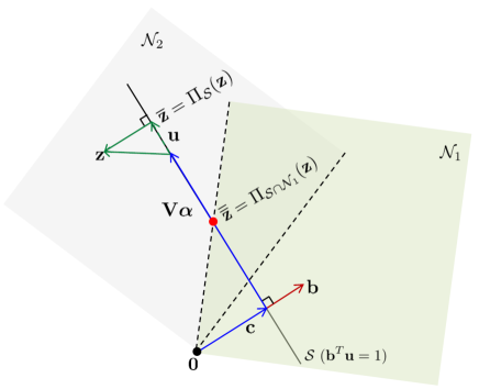
Figure 1: Illustration of the projection of $\bf z$ onto the set ${\cal S}\cap{\cal N}_{1}$: the set $\cal S$ is defined by the vector ${\bf c}\in\cal S$ and by the vector $\bf b$ orthogonal to the subspace ${\cal S}-\{\bf c\}$; the vector ${\bf u}\in\cal S$ may be written as ${\bf u=V}\bm{\alpha}+{\bf c}$ where $\bf V$ spans the subspace ${\cal S}-\{\bf c\}$ and $\bm{\alpha}\in\mathbb{R}^{(m-1)}$; the vector $\overline{\bf z}$ is the orthogonal projection of $\bf z$ onto $\cal S$; the vector $\overline{\overline{\bf z}}$ is the orthogonal projection of $\overline{\bf z}$ onto ${\cal S}\cap{\cal N}_{1}$, which is also the orthogonal projection of $\bf z$ onto the set ${\cal S}\cap{\cal N}_{1}$.

To solve the optimization (13), we start by removing the constraint ${\mathbf{b}}^{T}{\mathbf{u}}=1$ by an appropriate change of variables. Having in mind that the set ${\cal S}=\{{\bf u}\in\mathbb{R}^{m}:{\bf b}^{T}{\bf u}=1\,\}$ is a hyperplane that contains the vector ${\bf c}={\bf b}/\|{\bf b}\|^{2}_{2}$, then that constraint is equivalent to ${{\mathbf{u}}={{\mathbf{c}}}}+{{\mathbf{V}}}\bm{\alpha}$, where $\bm{\alpha}\in\mathbb{R}^{m-1}$ and the columns of ${\bf V}\in\mathbb{R}^{m\times(m-1)}$ span the subspace ${\cal S}-\{{\mathbf{c}}\}=\{{{\mathbf{u}}}\in\mathbb{R}^{m}\,:{{\mathbf{b}}}^{T}{{\mathbf{u}}}=0\,\}$, of dimension $(m-1)$. The matrix ${\bf V}$ is chosen such that ${\bf V}^{T}{\bf V}={\bf I}_{m-1}$, i.e., the columns of $\bf V$ are orthonormal. Fig. 1 schematizes the mentioned entities jointly with $\overline{\bf z}$, the orthogonal projection of $\bf z$ onto $\cal S$, and $\overline{\overline{\bf z}}$, the orthogonal projection of $\overline{\bf z}$ onto ${\cal S}_{1}\cap{\cal N}_{1}$. The former projection may be written as

$$\overline{\bf z} \equiv\Pi_{\cal S}({\bf z})$$

$$={\bf c}+{\bf P}({\bf z-c})$$ (14)

where ${\bf P}\equiv{\bf VV}^{T}={{\mathbf{I}}}_{m}-{\bf bb}^{T}/\|{\bf b}\|_{2}^{2}$ denotes the orthogonal projection matrix onto ${\cal S}-\{\bf c\}$. With these objects in place, and given ${\bf z}\in\mathbb{R}^{m}$ and $\bf u\in{\cal S}$, we simplify the cost function $\|{\bf z-u}\|^{2}_{2}$ by introducing the projection of $\bf z$ onto $\cal S$ and by using the Pythagorean theorem as follows:

$$\|{\bf z-u}\|_{2}^{2} =\|{\bf z}-\overline{\bf z}\|_{2}^{2}+\|\overline{\bf z}-{\bf u}\|_{2}^{2}$$

$$=\|{\bf z}-\overline{\bf z}\|_{2}^{2}+\|(\overline{\bf z}-{\bf c})-{\bf V}\bm{\alpha}\|_{2}^{2}$$

$$=\|{\bf z}-\overline{\bf z}\|_{2}^{2}+\|{\bf V}^{T}({\bf z-c})-\bm{\alpha}\|_{2}^{2}$$ (15)

where the right hand term in (15) derives directly from (14) and from the fact that ${\bf V}^{T}{\bf V}={\bf I}_{m-1}$. By introducing ${\bf u=c+V}\bm{\alpha}$ in (13), we obtain the equivalent optimization

$$\min\limits_{\bm{\alpha}}\|{\bf V}^{T}({\bf z-c})-\bm{\alpha}\|_{2}^{2}\;\;\textrm{s.t.}\;\;({\bf V}^{T}{\bf d}_{i})^{T}\bm{\alpha}\geq-({\bf d}_{i}^{T}{\bf c})$$ (16)

which is a projection onto a half space whose solution is [24]

$$\bm{\alpha}^{*}={\bf V}^{T}({\bf z-c})+\tau_{i}\frac{{\bf V}^{T}{\bf d}_{i}}{\|{\bf V}^{T}{\bf d}_{i}\|_{2}}$$

where

$$\tau_{i} =\max\left\{0,-\frac{{\bf d}_{i}^{T}{\bf V}}{\|{\bf V}^{T}{\bf d}_{i}\|_{2}}\big{(}{\bf V}^{T}({\bf z-c})\big{)}-\frac{{\bf d}_{i}^{T}{\bf c}}{\|{\bf V}^{T}{\bf d}_{i}\|_{2}}\right\}$$

$$=\max\{0,-{\bf s}_{i}^{T}{\bf z}+f_{i}\}$$

with ${\bf s}_{i}\equiv{\bf Pd}_{i}/\|{\bf Pd}_{i}\|_{2}$, $f_{i}\equiv-{\bf d}_{i}^{T}{\bf c}/\|{\bf P}{\bf d}_{i}\|_{2}$, and we have used the facts that $\|{\bf V}^{T}{\bf x}\|_{2}=\|{\bf P}{\bf x}\|_{2}$ and ${\bf V}^{T}{\bf c}=\bf 0$.

Recalling that ${\bf u={\bf c}}+{\bf V}\bm{\alpha}$, we obtain

$$\begin{split}\overline{\overline{\bf z}}&={\bf c}+{\bf VV}^{T}({\bf z-c})+\tau_{i}{\bf s}_{i}\\ &=\Pi_{\cal S}({\bf z})+\tau_{i}{\bf s}_{i}.\end{split}$$ (17)

The interpretation of (17) is clear: the orthogonal projection of $\bf z$ onto ${\cal S}\cap{\cal N}_{i}$ is obtained by first computing $\overline{\bf z}=\Pi_{\cal S}({\bf z})$, i.e.. the projection ${\bf z}$ onto the hyperplane $\cal S$, and then computing $\overline{\overline{\bf z}}=\Pi_{{\cal S}\cap{\cal N}_{i}}(\overline{\bf z})$, i.e.. the projection $\overline{\bf z}$ onto the intersection ${\cal S}\cap{\cal N}_{i}$. Given that ${\cal S}\cap{\cal N}_{i}\subset{\cal S}$, then (17) is, essentially, a consequence of a well know result: given a convex set contained in some subspace, then the orthogonal projection of any point in the convex set can be accomplished by first projecting orthogonally on that subspace, and then projecting the result on the convex set [31, Ch. 5.14].

Finally, computing ${\bf U}^{*}_{i}$ can be conducted in parallel for each column of ${\mathbf{Z}}$ leading to the following matrix update rule summarized in Algorithm 3):

$${\bf U}^{*}_{i} =\Pi_{\cal S}({\bf Z})+{\bf s}_{i}\bm{\tau}_{i}^{T}$$ (18)

with $\bm{\tau}_{i}^{T}\in\mathbb{R}^{1\times n}$ given by

$$\bm{\tau}_{i}^{T}=\max\{{\bf 0},f_{i}{\bf 1}_{n}^{T}-{\bf s}_{i}^{T}{\bf Z}\}$$

where

$$f_{i} =-\frac{{\bf d}_{i}^{T}{\bf c}}{\|{\bf Pd}_{i}\|_{2}}$$ (19)

and the operator $\max$ has to be understood in the component-wise sense

Input: ${\mathbf{Z}}$, ${\mathbf{b}}$, ${\mathbf{d}}_{i}$

// Calculate ${\mathbf{P}}{\mathbf{d}}_{i}$, ${\mathbf{s}}_{i}$, ${\mathbf{c}}$ and $f_{i}$

1 ${\mathbf{c}}\leftarrow{\mathbf{b}}/\|{\bf b}\|^{2}_{2}$;

2 ${\mathbf{P}}{\mathbf{d}}_{i}\leftarrow{\mathbf{d}}_{i}-{\bf cb}^{T}{\mathbf{d}}_{i}$;

3 ${\mathbf{s}}_{i}\leftarrow{\mathbf{P}}{\mathbf{d}}_{i}/\|{\mathbf{P}}{\mathbf{d}}_{i}\|_{2}$ ;

4 $f_{i}\leftarrow-{{\bf d}_{i}^{T}{\bf c}}/{\|{\mathbf{P}}{\mathbf{d}}_{i}\|_{2}}$ ;

// Calculate $\bm{\tau}_{i}^{T}$

5 $\bm{\tau}_{i}^{T}\leftarrow\max\{{\bf 0},f_{i}{\bf 1}_{n}^{T}-{\bf s}_{i}^{T}{\bf Z}\}$;

6

// Project ${\mathbf{Z}}$ onto ${\mathcal{S}}$

7 $\Pi_{\cal S}({\bf Z})\leftarrow{\bf c}{\bf 1}_{n}^{T}+{\bf P}({\mathbf{Z}}-{\bf c}{\bf 1}_{n}^{T})$;

// Compute the final solution ${\mathbf{U}}_{i}^{\ast}$

8 ${\mathbf{U}}_{i}^{\ast}\leftarrow\Pi_{\cal S}({\bf Z})+{\bf s}_{i}\bm{\tau}_{i}^{T}$;

Output: ${\mathbf{U}}_{i}^{\ast}$

Algorithm 3 Projecting ${\mathbf{Z}}$ onto ${\mathcal{S}}\cap{\mathcal{N}}_{i}$

Note that using the Karush-Kuhn-Tucker (KKT) conditions to solve the problem (13) can also lead to this exact solution, as described in the Appendix.

II-D Convergence Analysis

The convergence of the Dykstra’s projection was first proved in [28], where it was claimed that the sequences generated using Dykstra’s algorithm are guaranteed to converge to the projection of the original point onto the intersection of the convex sets. Its convergence rate was explored later [32, 33]. We now recall the Deutsch-Hundal theorem providing the convergence rate of the projection onto the intersection of $m$ closed half-spaces.

Theorem 1 (Deutsch-Hundal, [32]; Theorem 3.8).

Assuming that ${\mathbf{X}}_{k}$ is the $k$th projected result in Dykstra’s algorithm and ${\mathbf{X}}_{\infty}$ is the converged point, there exist constants $0\leq c<1$ and $\rho>0$ such that

$$\|{\mathbf{X}}_{k}-{\mathbf{X}}_{\infty}\|_{F}^{2}\leq\rho c^{k}$$ (20)

for all $k$.

Theorem 1 demonstrates that Dykstra’s projection has a linear convergence rate [34]. The convergence speed depends on the constant $c$, which depends on the number of constraints $m$ and the ‘angle’ between two half-spaces [32]. To the best of our knowledge, the explicit form of $c$ only exists for $m=2$ half-spaces and its determination for $m>2$ is still an open problem [35].

II-E Complexity Analysis

To summarize, the projection onto ${\mathcal{S}}\cap{\mathcal{N}}$ can be obtained by iteratively projecting onto the $m$ sets ${\mathcal{S}}\cap{\mathcal{N}}_{i}$ ($i=1,\ldots,m$) using a Dykstra’s projection scheme as described in Algorithm 2. The output of this algorithm converges to the projection of the initial point ${\mathbf{Y}}$ onto ${\mathcal{S}}\cap{\mathcal{N}}$. It is interesting to note that the quantities denoted as $\Pi_{\cal S}({\bf Z})$ in Algorithm 3 needs to be calculated only once since the projection of ${\mathbf{Z}}$ will be itself ${\mathbf{Z}}$ from the second projection $\Pi_{{\mathcal{S}}\cap{\mathcal{N}}_{2}}$. This results from the fact that the projection never jumps out from the hyperplane ${\mathcal{S}}$.

Moreover, the most computationally expensive part of the proposed unmixing algorithm (Algorithm 1) is the iterative procedure to project onto ${\mathcal{S}}\cap{\mathcal{N}}$, as described in Algorithm 2. For each iteration, the heaviest step is the projection onto the intersection ${\mathcal{S}}\cap{\mathcal{N}}_{i}$ summarized in Algorithm 3. With the proposed approach, this projection only requires vector products and sums, with a cost of $\mathcal{O}(nm)$ operations, contrary to the $\mathcal{O}(nm^{2})$ computational cost of [22]. Thus, each iteration of Algorithm 2 has a complexity of order $\mathcal{O}(nm^{2})$.

III Experiments using Synthetic and Real Data

This section compares the proposed unmixing algorithm with several state-of-the-art unmixing algorithms, i.e., FCLS [17], SUNSAL [20], IPLS [21] and APU [22]. All algorithms have been implemented using MATLAB R2014A on a computer with Intel(R) Core(TM) i7-2600 CPU@3.40GHz and 8GB RAM. To conduct a fair comparison, they have been implemented in the signal subspace without using any parallelization. These unmixing algorithms have been compared using the figures of merit described in Section III-A. Several experiments have been conducted using synthetic datasets and are presented in Section III-B. Two real hyperspectral (HS) datasets associated with two different applications are considered in Section III-C. The MATLAB codes and all the simulation results are available on the first author’s homepage.

III-A Performance Measures

In what follows, $\widehat{\bf A}_{t}$ denotes the estimation of ${\mathbf{A}}$ obtained at time $t$ (in seconds) for a given algorithm. Provided that the endmember matrix $\bf E$ has full column rank, the solution of (4) is unique and all the algorithms are expected to converge to this unique solution, denoted as ${\mathbf{A}}^{\star}\triangleq\widehat{\bf A}_{\infty}$ (ignoring numerical errors). In this work, one of the state-of-the-art methods is run with a large number of iterations ($n=5000$ in our experiments) to guarantee that the optimal point ${\mathbf{A}}^{\star}$ has been reached.

III-A1 Convergence Assessment

First, different solvers designed to compute the solution of (4) have been compared w.r.t. the time they require to achieve a given accuracy. Thus, all these algorithms have been run on the same platform and we have evaluated the relative error (RE) between $\widehat{{\mathbf{A}}}_{t}$ and ${\mathbf{A}}^{\star}$ as a function of the computational time defined as

$$\text{RE}_{t}=\frac{\|\widehat{\bf A}_{t}-{\bf A}^{\star}\|^{2}_{F}}{\|{{\mathbf{A}}}^{\star}\|^{2}_{F}}.$$

III-A2 Quality Assessment

To analyze the quality of the unmixing results, we have also considered the normalized mean square error (NMSE)

$$\textrm{NMSE}_{t}=\frac{\|\widehat{\bf A}_{t}-{\bf A}\|^{2}_{F}}{\|{\bf A}\|^{2}_{F}}.$$

The smaller NMSE_t, the better the quality of the unmixing. Note that $\text{NMSE}_{\infty}=\frac{\|{{\mathbf{A}}}^{\star}-{\mathbf{A}}\|^{2}_{F}}{\|{\mathbf{A}}\|^{2}_{F}}$ is a characteristic of the objective criterion (4) and not of the algorithm.

III-B Unmixing Synthetic Data

The synthetic data is generated using endmember spectra selected from the United States Geological Survey (USGS) digital spectral library. These reflectance spectra consists of $L=224$ spectral bands from $383$nm to $2508$nm. To mitigate the impact of the intra-endmember correlation, three different subsets ${\mathbf{E}}_{3}$, ${\mathbf{E}}_{10}$ and ${\mathbf{E}}_{20}$ have been built from this USGS library. More specifically, ${\mathbf{E}}_{\alpha}$ is an endmember matrix in which the angle between any two different columns (endmember signatures) is larger than $\alpha$ (in degree). Thus, the smaller $\alpha$, the more similar the endmembers and the higher the conditioning number of ${\mathbf{E}}$. For example, ${\mathbf{E}}_{3}$ contains similar endmembers with very small variations (including scalings) of the same materials and ${\mathbf{E}}_{20}$ contains endmembers which are relatively less similar. As an illustration, a random selection of several endmembers from ${\mathbf{E}}_{3}$ and ${\mathbf{E}}_{20}$ have been depicted in Fig. 2. The abundances have been generated uniformly in the simplex ${\mathcal{A}}$ defined by the ANC and ASC constraints.

Unless indicated, the performance of these algorithms has been evaluated on a synthetic image of size ${100}\times{100}$ whose signal to noise ratio (SNR) has been fixed to SNR=$30$dB and the number of considered endmembers is $m=5$.

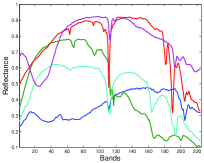
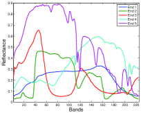
Figure 2: Five endmember signatures randomly selected from ${\mathbf{E}}_{3}$ (left) and ${\mathbf{E}}_{20}$ (right).

III-B1 Initialization

The proposed SUDAP, APU and FCLS algorithms do not require any initialization contrary to SUNSAL and IPLS. As suggested by the authors of these two methods, SUNSAL has been initialized with the unconstrained LS estimator of the abundances whereas IPLS has been initialized with the zero matrix. Note that our simulations have shown that both SUNSAL and IPLS are not sensitive to these initializations.

III-B2 Performance vs. Time

The NMSE and RE for these five different algorithms are displayed in Fig. 3 as a function of the execution time. These results have been obtained by averaging the outputs of $30$ Monte Carlo runs. More precisely, 10 randomly selected matrices for each set ${\mathbf{E}}_{3}$, ${\mathbf{E}}_{10}$ and ${\mathbf{E}}_{20}$ are used to consider the different intra-endmember correlations. All the algorithms converge to the same solution as expected. However, as demonstrated in these two figures, SUNSAL, APU and the proposed SUDAP are much faster than FCLS and IPLS. From the zoomed version in Fig. 3, we can observe that in the first iterations SUDAP converges faster than APU and SUNSAL. More specifically, for instance, if the respective algorithms are stopped once RE${}_{t}<-80$dB (around $t=50$ms), SUDAP performs faster than SUNSAL and APU and with a lower NMSE_t.

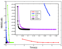
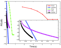
Figure 3: NMSE (left) and RE (right) vs. time (zoomed version in top right).

III-B3 Time vs. the Number of Endmembers

In this test, the number of endmembers $m$ varies from $3$ to $23$ while the other parameters have been fixed to the same values as in Section III-B2 (SNR$=30$dB and $n=100^{2}$). The endmember signatures have been selected from ${\mathbf{E}}_{10}$ (similar results have been observed when using ${\mathbf{E}}_{3}$ and ${\mathbf{E}}_{20}$). All the algorithms have been stopped once $\hat{{\mathbf{A}}}_{t}$ reaches the same convergence criterion RE${}_{t}<-100$dB. The proposed SUDAP has been compared with the two most competitive algorithms SUNSAL and APU. The final REs and the corresponding computational times versus $m$ have been reported in Fig. 4, including error bars to monitor the stability of the algorithms (these results have been computed from $30$ Monte Carlo runs).

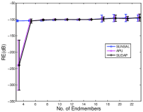
Figure 4: RE (left) and time (right) vs. number of endmembers for SUNSAL, APU and SUDAP (RE${}_{t}<-100$dB).

Fig. 4 (left) shows that all the algorithms have converged to a point satisfying RE${}_{t}<-100$dB and that SUDAP and APU are slightly better than SUNSAL. However, SUNSAL provides a smaller estimation variance leading to a more stable estimator. Fig. 4 (right) shows that the execution time of the three methods is an increasing function of the number of endmembers $m$, as expected. However, there are significant differences between the respective rates of increase. The execution times of APU and SUDAP are cubic and quadratic functions of $m$ whereas SUNSAL benefits from a milder increasing rate. More precisely, SUDAP is faster than SUNSAL when the number of endmembers is small, e.g., smaller than $19$ (this value may change depending on the SNR value, the conditioning number of $\bf E$, the abundance statistics, etc.). Conversely, SUNSAL is faster than SUDAP for $m\geq 19$. SUNSAL is more efficient than APU for $m\geq 15$ and SUDAP is always faster than APU. The error bars confirm that SUNSAL offers more stable results than SUDAP and APU. Therefore, it can be concluded that the proposed SUDAP is more promising to unmix a multi-band image containing a reasonable number of materials, while SUNSAL is more efficient when considering a scenario containing a lot of materials.

III-B4 Time vs. Number of Pixels

In this test, the performance of the algorithms has been evaluated for a varying number of pixels $n$ from $100^{2}$ to $400^{2}$ (the other parameters have been fixed the same values as in Section III-B2). The endmember signatures have been selected from ${\mathbf{E}}_{10}$ (similar results have been observed when using ${\mathbf{E}}_{3}$ and ${\mathbf{E}}_{20}$) and the stopping rule has been chosen as RE${}_{t}<-100$dB. All results have been averaged from $30$ Monte Carlo runs. The final REs and the corresponding computational times are shown in Fig. 5. The computational time of the three algorithms increases approximately linearly w.r.t. the number of image pixels and SUDAP provides the faster solution, regardless the number of pixels.

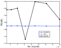
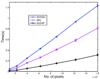
Figure 5: RE (left) and time (right) vs. number of pixels for SUNSAL, APU and SUDAP (RE${}_{t}<-100$dB).

III-B5 Time vs. SNR

In this experiment, the SNR of the HS image varies from $0$dB to $50$dB while the other parameters are the same as in Section III-B2. The stopping rule is the one of Section III-B3. The results are displayed in Fig. 6 and indicate that SUNSAL is more efficient than APU and SUDAP (i.e., uses less time) for low SNR scenarios. More specifically, to achieve RE${}_{t}<-100$dB, SUNSAL provides more efficient unmixing when the SNR is lower than $5$dB while SUDAP is faster than SUNSAL when the SNR is higher than $5$dB.

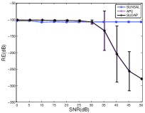
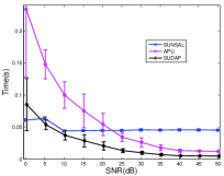
Figure 6: RE (left) and time (right) vs. SNR for SUNSAL, APU and SUDAP (RE${}_{t}<-100$dB).

III-C Real Data

This section compares the performance of the proposed SUDAP algorithm with that of SUNSAL and APU using two real datasets associated with two different applications, i.e., spectroscopy and hyperspectral imaging.

III-C1 EELS Dataset

In this experiment, a spectral image acquired by electron energy-loss spectroscopy (EELS) is considered. The analyzed dataset is a $64\times 64$ pixel spectrum-image acquired in $n_{\lambda}=1340$ energy channels over a region composed of several nanocages in a boron-nitride nanotubes (BNNT) sample [3]. A false color image of the EELS data (with an arbitrary selection of three channels as RGB bands) is displayed in Fig. 7 (left). Following [3], the number of endmembers has been set to $m=6$. The endmember signatures have been extracted from the dataset using VCA [15] and are depicted in Fig. 7 (right). The abundance maps estimated by the considered unmixing algorithms are shown in Fig. 8 for a stopping rule defined as RE${}_{t}<100$dB.

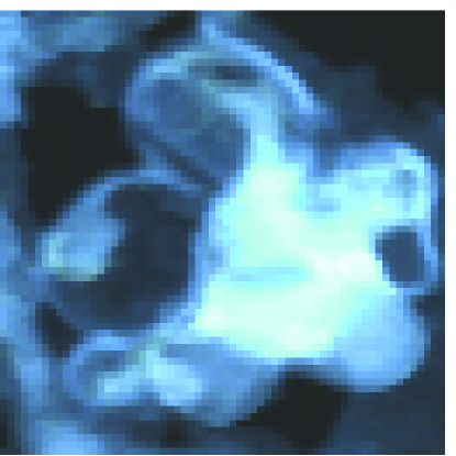
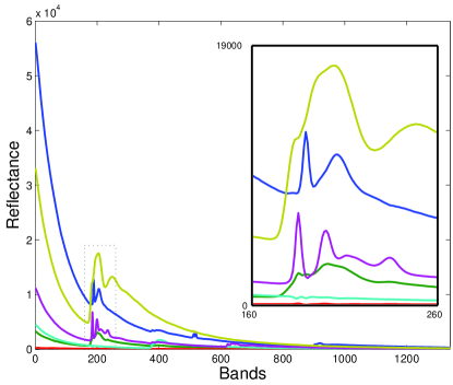
Figure 7: EELS dataset: HS image (left) and extracted endmember signatures (right).

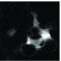
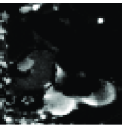
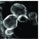
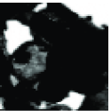
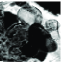
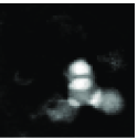
Figure 8: EELS dataset: abundance maps estimated by SUNSAL (top), APU (middle) and SUDAP (bottom).

There is no visual difference between the abundance maps provided by SUNSAL, APU and the proposed SUDAP. Since there is no available ground-truth for the abundances, the objective criterion ${\mathcal{J}}_{t}=\|{\mathbf{X}}-{\mathbf{E}}\hat{{\mathbf{A}}}_{t}\|_{F}^{2}$ minimized by the algorithms has been evaluated instead of NMSE_t. The variations of the objective function and the corresponding REs are displayed in Fig. 9 as a function of the computational time.

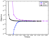
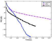
Figure 9: Objective (left) and RE (right) vs. time for SUNSAL, APU and SUDAP (EELS data).

Both figures show that the proposed SUDAP performs faster than APU and SUNSAL as long as the stopping rule has been fixed as RE${}_{t}<-60$dB. For lower RE_t, SUDAP becomes less efficient than SUNSAL. To explore the convergence more explicitly, the number of spectral vectors that do not satisfy the convergence criterion, i.e., for which RE$>-100$dB, has been determined and is depicted in Fig. 10. It is clear that most of the spectral vectors (around $3600$ out of $4096$ pixels) converged quickly, e.g., in less than $0.02$ seconds. The remaining measurements (around $500$ pixels) require longer time to converge, which leads to the slow convergence as observed in Fig. 9. The slow convergence of the projection methods for these pixels may result from an inappropriate observational model due to, e.g., endmember variability [36] or nonlinearity effects [9]. On the contrary, SUNSAL is more robust to these discrepancies and converges faster for these pixels. This corresponds to the results shown in Fig. 9.

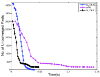
Figure 10: Number of pixels that do not satisfy the stopping rule vs. time for SUNSAL, APU and SUDAP (EELS data).

III-C2 Cuprite Dataset

This section investigates the performance of the proposed SUDAP algorithm when unmixing a real HS image. This image, which has received a lot of interest in the remote sensing and geoscience literature, was acquired over Cuprite field by the JPL/NASA airborne visible/infrared imaging spectrometer (AVIRIS) [37]. Cuprite scene is a mining area in southern Nevada composed of several minerals and some vegetation, located approximately $200$km northwest of Las Vegas. The image considered in this experiment consists of $250\times 190$ pixels of $n_{\lambda}=189$ spectral bands obtained after removing the water vapor absorption bands. A composite color image of the scene of interest is shown in Fig. 11 (left). As in Section III-C2, the endmember matrix ${\mathbf{E}}$ has been learnt from the HS data using VCA. According to [15], the number of endmembers has been set to $m=14$. The estimated endmember signatures are displayed in Fig. 11 (right) ant the first five corresponding abundance maps recovered by SUNSAL, APU and SUDAP are shown in Fig. 12. Visually, all three methods provide similar abundance maps.

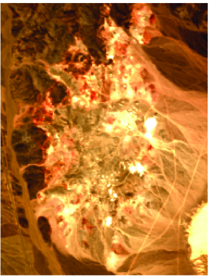
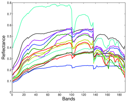
Figure 11: Cuprite dataset: HS image (left) and extracted endmember signatures (right).

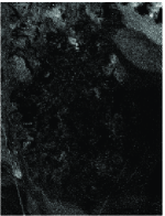
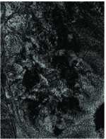
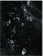
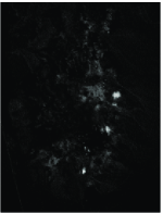
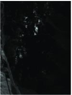
Figure 12: Cuprite dataset: abundance maps estimated by SUNSAL (top), APU (middle) and SUDAP (bottom).

From Fig. 11 (right), the signatures appear to be highly correlated, which makes the unmixing quite challenging. This can be confirmed by computing the smallest angle between any couple of endmembers, which is equal to $\alpha=2.46$ (in degree). This makes the projection-based methods, including SUDAP and APU, less efficient since alternating projections are widely known for their slower convergence when the convex sets exhibit small angles, which is consistent with the convergence analysis in Section II-D. Fig. 13, which depicts the objective function and the RE w.r.t. the computational times corroborates this point. Indeed, SUDAP performs faster than SUNSAL and APU if the algorithms are stopped before RE$<-30$dB. For lower RE_t, SUNSAL surpasses SUDAP.

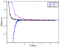
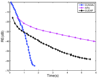
Figure 13: Objective function (left) and RE (right) vs. time for SUNSAL, APU and SUDAP (Cuprite data).

IV Conclusion

This paper proposed a fast unmixing method based on an alternating projection strategy. Formulating the spectral unmixing problem as a projection onto the intersection of convex sets allowed Dykstra’s algorithm to be used to compute the solution of this unmixing problem. The projection was implemented intrinsically in a subspace, making the proposed algorithm computationally efficient. In particular, the proposed unmixing algorithm showed similar performance comparing to state-of-the-art methods, with significantly reduced execution time, especially when the number of endmembers is small or moderate, which is often the case when analyzing conventional multi-band images. Future work includes the generalization of the proposed algorithm to cases where the endmember matrix is rank deficient or ill-conditioned.

[Solving (13) with KKT conditions] Following the KKT conditions, the problem (13) can be reformulated as finding ${\mathbf{u}}^{\ast}$ satisfying the following conditions

$$\begin{array}[]{rcl}{\mathbf{u}}^{\ast}-{\mathbf{z}}+\mu{\mathbf{b}}-\lambda{\mathbf{d}}_{i}&=&\bm{0}\\ {\mathbf{d}}_{i}^{T}{\mathbf{u}}^{\ast}&\geq&0\\ {\mathbf{b}}^{T}{\mathbf{u}}^{\ast}&=&1\\ \lambda&\geq&0\\ \mu&\geq&0\\ \lambda{\mathbf{d}}_{i}^{T}{\mathbf{u}}^{\ast}&=&0.\end{array}$$ (21)

Direct computations lead to

$${\mathbf{u}}^{\ast}={\mathbf{z}}-\tilde{{\mathbf{z}}}+\Delta{\mathbf{z}}$$ (22)

where

$$\begin{array}[]{rcl}\tilde{{\mathbf{z}}}&=&{\mathbf{c}}\left({\mathbf{b}}^{T}{\mathbf{z}}-1\right)\\ {\mathbf{c}}&=&{\mathbf{b}}/\left\|{\mathbf{b}}\right\|^{2}_{2}\\ \Delta{\mathbf{z}}&=&\tau_{i}{\mathbf{s}}_{i}\\ \tau_{i}&=&\max\{0,-{\mathbf{d}}_{i}^{T}\left({\mathbf{z}}-\tilde{{\mathbf{z}}}\right)/\|{\mathbf{P}}{\mathbf{d}}_{i}\|_{2}\}\\ {\mathbf{s}}_{i}&=&{\mathbf{P}}{\mathbf{d}}_{i}/\|{\mathbf{P}}{\mathbf{d}}_{i}\|_{2}\\ {\mathbf{P}}&=&\textbf{I}_{m}-{\mathbf{b}}{\mathbf{b}}^{T}/\left\|{\mathbf{b}}\right\|^{2}_{2}.\\ \end{array}$$ (23)

Computing the projection of ${\mathbf{z}}_{j}$ for $j=1,\cdots,n$ can be conducted in parallel, leading to the following matrix update rule

$$\begin{array}[]{ll}{\mathbf{U}}_{i}^{\ast}&=\Pi_{{\mathcal{S}}\cap{\mathcal{N}}_{i}}({\mathbf{Z}})\\ &={\mathbf{Z}}-\tilde{{\mathbf{Z}}}+{\mathbf{s}}_{i}\bm{\tau}_{i}^{T}\\ &=\Pi_{{\mathcal{S}}}{({\mathbf{Z}})}+{\mathbf{s}}_{i}\bm{\tau}_{i}^{T}\end{array}$$ (24)

where

$$\begin{split}&\tilde{{\mathbf{Z}}}={\mathbf{c}}\left({\mathbf{b}}^{T}{\mathbf{Z}}-\bm{1}_{n}^{T}\right)\\ &\bm{\tau}_{i}^{T}=\max\{{\bf 0},-{\mathbf{d}}_{i}^{T}\left({\mathbf{Z}}-\tilde{{\mathbf{Z}}}\right)/\|{\mathbf{P}}{\mathbf{d}}_{i}\|_{2}\}.\\ \end{split}$$

As a conclusion, the updating rules (24) and (18) only differ by the way the projection $\Pi_{{\mathcal{S}}}{({\mathbf{Z}})}$ onto ${\mathcal{S}}$ has been computed. However, it is easy to show that $\Pi_{{\mathcal{S}}}{({\mathbf{Z}})}={\mathbf{Z}}-\tilde{{\mathbf{Z}}}$ used in (24) is fully equivalent to $\Pi_{{\mathcal{S}}}{({\mathbf{Z}})}={\bf c}{\bf 1}_{n}^{T}+{\bf P}({\mathbf{Z}}-{\bf c}{\bf 1}_{n}^{T})$ required in (18).

Remark.

It is worthy to provide an alternative geometric interpretation of the KKT-based solution (22). First, ${\mathbf{z}}-\tilde{{\mathbf{z}}}$ is the projection of ${\mathbf{z}}$ onto the affine set ${\mathcal{S}}$. Second, if the projection is inside the set ${\mathcal{N}}_{i}$, which means ${\mathbf{d}}_{i}^{T}\left({\mathbf{z}}-\tilde{{\mathbf{z}}}\right)\geq 0$, then the projection of ${\mathbf{z}}$ onto the intersection ${\mathcal{S}}\cap{\mathcal{N}}_{i}$ is ${\mathbf{z}}-\tilde{{\mathbf{z}}}$. If the projection is outside of the set ${\mathcal{N}}_{i}$, implying that ${\mathbf{d}}_{i}^{T}\left({\mathbf{z}}-\tilde{{\mathbf{z}}}\right)<0$, a move $\Delta{\mathbf{z}}$ inside the affine set ${\mathcal{S}}$ should be added to ${\mathbf{z}}-\tilde{{\mathbf{z}}}$ to reach the set ${\mathcal{N}}_{i}$. This move $\Delta{\mathbf{z}}$ should ensure three constraints: 1) $\Delta{\mathbf{z}}$ keeps the point ${\mathbf{z}}-\tilde{{\mathbf{z}}}+\Delta{\mathbf{z}}$ inside the affine set ${\mathcal{S}}$, 2) ${\mathbf{z}}-\tilde{{\mathbf{z}}}+\Delta{\mathbf{z}}$ is on the boundary of the set ${\mathcal{N}}_{i}$, and 3) the Euclidean norm of $\Delta{\mathbf{z}}$ is minimal. The first constraint, which can be formulated as ${\mathbf{b}}^{T}\Delta{\mathbf{z}}=0$, is ensured by imposing a move of the form $\Delta{\mathbf{z}}={\mathbf{P}}{\mathbf{w}}$ where ${\mathbf{P}}={\mathbf{V}}{\mathbf{V}}^{T}$ is the projector onto the subspace ${\mathcal{S}}_{0}$ orthogonal to ${\mathbf{b}}$. The second constraint is fulfilled when ${\mathbf{d}}_{i}^{T}\left({\mathbf{z}}-\tilde{{\mathbf{z}}}+\Delta{\mathbf{z}}\right)=0$, leading to ${{\mathbf{d}}_{i}^{T}}{{\mathbf{P}}{\mathbf{w}}}=-\delta_{i}$, where $\delta_{i}={\mathbf{d}}_{i}^{T}\left({\mathbf{z}}-\tilde{{\mathbf{z}}}\right)$. Thus, due to the third constraint, ${\mathbf{w}}$ can be defined as

$${\mathbf{w}}=\operatornamewithlimits{argmin}_{\bf v}\|{\bf Pv}\|_{2}^{2}\ \textrm{ s.t. }\ {\mathbf{d}}_{i}^{T}{\mathbf{P}}{\mathbf{w}}=-\delta_{i}.$$ (25)

Using the fact that ${\mathbf{P}}$ is an idempotent matrix, i.e., ${\mathbf{P}}^{2}={\mathbf{P}}$, the constrained optimization problem can be solved analytically with the method of Lagrange multipliers, leading to

$${\mathbf{w}}={-\delta_{i}}{\left({\mathbf{d}}_{i}^{T}{\mathbf{P}}{\mathbf{d}}_{i}\right)}^{-1}{\mathbf{d}}_{i}$$ (26)

and $\Delta{\mathbf{z}}={{\mathbf{P}}{\mathbf{w}}}={-\delta_{i}}{\left({\mathbf{d}}_{i}^{T}{\mathbf{P}}{\mathbf{d}}_{i}\right)}^{-1}{\mathbf{P}}{\mathbf{d}}_{i}$. This final result is consistent with the move defined in (22) and (23) by setting $\tau_{i}=\max\{0,-\frac{\delta_{i}}{\|{\mathbf{P}}{\mathbf{d}}_{i}\|_{2}}\}$ and ${\mathbf{s}}_{i}={\mathbf{P}}{\mathbf{d}}_{i}/\|{\mathbf{P}}{\mathbf{d}}_{i}\|_{2}$. Recall that $\left\|{\mathbf{P}}{\mathbf{d}}_{i}\right\|_{2}^{2}=\left({\mathbf{d}}_{i}^{T}{\mathbf{P}}{\mathbf{d}}_{i}\right)$ since ${\mathbf{P}}^{T}{\mathbf{P}}={\mathbf{P}}$.

References

- [1] A. Averbuch, M. Zheludev, and V. Zheludev, “Unmixing and target recognition in hyper-spectral imaging,” Earth Science Research, vol. 1, no. 2, pp. 200–228, 2012.
- [2] K. E. Themelis, F. Schmidt, O. Sykioti, A. A. Rontogiannis, K. D. Koutroumbas, and I. A. Daglis, “On the unmixing of MEx/OMEGA hyperspectral data,” Planetary and Space Science, vol. 68, no. 1, pp. 34–41, 2012.
- [3] N. Dobigeon and N. Brun, “Spectral mixture analysis of EELS spectrum-images,” Ultramicroscopy, vol. 120, pp. 25–34, Sept. 2012.
- [4] C. Carteret, A. Dandeu, S. Moussaoui, H. Muhr, B. Humbert, and E. Plasari, “Polymorphism studied by lattice phonon raman spectroscopy and statistical mixture analysis method. Application to calcium carbonate polymorphs during batch crystallization,” Crystal Growth & Design, vol. 9, no. 2, pp. 807–812, 2009.
- [5] Y. Huang, A. K. Zaas, A. Rao, N. Dobigeon, P. J. Woolf, T. Veldman, N. C. Oien, M. T. McClain, J. B. Varkey, B. Nicholson, L. Carin, S. Kingsmore, C. W. Woods, G. S. Ginsburg, and A. Hero, “Temporal dynamics of host molecular responses differentiate symptomatic and asymptomatic influenza A infection,” PLoS Genetics, vol. 8, no. 7, p. e1002234, Aug. 2011.
- [6] C.-I Chang, X.-L. Zhao, M. L. G. Althouse, and J. J. Pan, “Least squares subspace projection approach to mixed pixel classification for hyperspectral images,” IEEE Trans. Geosci. Remote Sens., vol. 36, no. 3, pp. 898–912, May 1998.
- [7] J. Wang and C.-I Chang, “Applications of independent component analysis in endmember extraction and abundance quantification for hyperspectral imagery,” IEEE Trans. Geosci. Remote Sens., vol. 4, no. 9, pp. 2601–2616, Sept. 2006.
- [8] D. Manolakis, C. Siracusa, and G. Shaw, “Hyperspectral subpixel target detection using the linear mixing model,” IEEE Trans. Geosci. Remote Sens., vol. 39, no. 7, pp. 1392–1409, July 2001.
- [9] N. Dobigeon, J.-Y. Tourneret, C. Richard, J. C. M. Bermudez, S. McLaughlin, and A. O. Hero, “Nonlinear unmixing of hyperspectral images: Models and algorithms,” IEEE Signal Process. Mag., vol. 31, no. 1, pp. 89–94, Jan. 2014.
- [10] N. Keshava and J. F. Mustard, “Spectral unmixing,” IEEE Signal Process. Mag., vol. 19, no. 1, pp. 44–57, Jan. 2002.
- [11] J. Bioucas-Dias, A. Plaza, N. Dobigeon, M. Parente, Q. Du, P. Gader, and J. Chanussot, “Hyperspectral unmixing overview: Geometrical, statistical, and sparse regression-based approaches,” IEEE J. Sel. Topics Appl. Earth Observ. Remote Sens., vol. 5, no. 2, pp. 354–379, Apr. 2012.
- [12] W.-K. Ma, J. M. Bioucas-Dias, T.-H. Chan, N. Gillis, P. Gader, A. J. Plaza, A. Ambikapathi, and C.-Y. Chi, “A signal processing perspective on hyperspectral unmixing: Insights from remote sensing,” IEEE Signal Process. Mag., vol. 31, no. 1, pp. 67–81, 2014.
- [13] F. Schmidt, A. Schmidt, E. Tréguier, M. Guiheneuf, S. Moussaoui, and N. Dobigeon, “Implementation strategies for hyperspectral unmixing using bayesian source separation,” IEEE Trans. Geosci. Remote Sens., vol. 48, no. 11, pp. 4003–4013, 2010.
- [14] M. E. Winter, “N-FINDR: an algorithm for fast autonomous spectral end-member determination in hyperspectral data,” in Proc. SPIE Imaging Spectrometry V, M. R. Descour and S. S. Shen, Eds., vol. 3753, no. 1. SPIE, 1999, pp. 266–275.
- [15] J. Nascimento and J. Bioucas-Dias, “Vertex component analysis: A fast algorithm to unmix hyperspectral data,” IEEE Trans. Geosci. Remote Sens., vol. 43, no. 4, pp. 898–910, 2005.
- [16] T.-H. Chan, W.-K. Ma, A. Ambikapathi, and C.-Y. Chi, “A simplex volume maximization framework for hyperspectral endmember extraction,” IEEE Trans. Geosci. Remote Sens., vol. 49, no. 11, pp. 4177–4193, 2011.
- [17] D. C. Heinz and C.-I. Chang, “Fully constrained least squares linear spectral mixture analysis method for material quantification in hyperspectral imagery,” IEEE Trans. Geosci. Remote Sens., vol. 39, no. 3, pp. 529–545, 2001.
- [18] C. L. Lawson and R. J. Hanson, Solving least squares problems. Englewood Cliffs, NJ: Prentice-hall, 1974, vol. 161.
- [19] N. Dobigeon, J.-Y. Tourneret, and C.-I Chang, “Semi-supervised linear spectral unmixing using a hierarchical Bayesian model for hyperspectral imagery,” IEEE Trans. Signal Process., vol. 56, no. 7, pp. 2684–2695, July 2008.
- [20] J. M. Bioucas-Dias and M. A. Figueiredo, “Alternating direction algorithms for constrained sparse regression: Application to hyperspectral unmixing,” in Proc. IEEE GRSS Workshop Hyperspectral Image SIgnal Process.: Evolution in Remote Sens. (WHISPERS), Reykjavik, Iceland, Jun. 2010, pp. 1–4.
- [21] E. Chouzenoux, M. Legendre, S. Moussaoui, and J. Idier, “Fast constrained least squares spectral unmixing using primal-dual interior-point optimization,” IEEE J. Sel. Topics Appl. Earth Observ. Remote Sens., vol. 7, no. 1, pp. 59–69, 2014.
- [22] R. Heylen, M. A. Akhter, and P. Scheunders, “On using projection onto convex sets for solving the hyperspectral unmixing problem,” IEEE Geosci. Remote Sens. Lett., vol. 10, no. 6, pp. 1522–1526, 2013.
- [23] J. P. Boyle and R. L. Dykstra, “A method for finding projections onto the intersection of convex sets in hilbert spaces,” in Advances in order restricted statistical inference. Springer, 1986, pp. 28–47.
- [24] S. Boyd and L. Vandenberghe, Convex optimization. Cambridge university press, 2004.
- [25] J. Duchi, S. Shalev-Shwartz, Y. Singer, and T. Chandra, “Efficient projections onto the for learning in high dimensions,” in Proc. Int. Conf. Machine Learning (ICML), Helsinki, Finland, 2008, pp. 272–279.
- [26] A. Kyrillidis, S. Becker, V. Cevher, and C. Koch, “Sparse projections onto the simplex,” in Proc. Int. Conf. Machine Learning (ICML), Atlanta, USA, 2013, pp. 235–243.
- [27] L. Condat, “Fast projection onto the simplex and the ball,” Preprint HAL-01056171, Aug. 2014. [Online]. Available: https://hal.archives-ouvertes.fr/hal-01056171/document
- [28] R. L. Dykstra, “An algorithm for restricted least squares regression,” J. Amer. Stat. Assoc., vol. 78, no. 384, pp. 837–842, 1983.
- [29] H. H. Bauschke and P. L. Combettes, “A Dykstra-like algorithm for two monotone operators,” Pacific Journal of Optimization, vol. 4, no. 3, pp. 383–391, 2008.
- [30] P. Combettes and J.-C. Pesquet, “Proximal splitting methods in signal processing,” in Fixed-Point Algorithms for Inverse Problems in Science and Engineering, ser. Springer Optimization and Its Applications, H. H. Bauschke, R. S. Burachik, P. L. Combettes, V. Elser, D. R. Luke, and H. Wolkowicz, Eds. Springer New York, 2011, pp. 185–212.
- [31] F. Deutsch, Best Approximation in Inner Product Spaces. Springer-Verlag, 2001.
- [32] F. Deutsch and H. Hundal, “The rate of convergence of Dykstra’s cyclic projections algorithm: The polyhedral case,” Numer. Funct. Anal. Optimization, vol. 15, no. 5-6, pp. 537–565, 1994.
- [33] S. Xu, “Estimation of the convergence rate of Dykstra’s cyclic projections algorithm in polyhedral case,” Acta Mathematicae Applicatae Sinica (English Series), vol. 16, no. 2, pp. 217–220, 2000.
- [34] S. J. Wright and J. Nocedal, Numerical optimization. Springer New York, 1999, vol. 2.
- [35] F. Deutsch and H. Hundal, “The rate of convergence for the cyclic projections algorithm III: regularity of convex sets,” J. Approx. Theory, vol. 155, no. 2, pp. 155–184, 2008.
- [36] A. Zare and K. Ho, “Endmember variability in hyperspectral analysis: Addressing spectral variability during spectral unmixing,” IEEE Signal Process. Mag., vol. 31, no. 1, pp. 95–104, 2014.
- [37] Jet Propulsion Lab. (JPL), “AVIRIS free data,” California Inst. Technol., Pasadena, CA, 2006. [Online]. Available: http://aviris.jpl.nasa.gov/html/aviris.freedata.html
- [38] Q. Wei, J. Bioucas-Dias, N. Dobigeon, and J.-Y. Tourneret, “Fast spectral unmixing based on Dykstra’s alternating projection – Complementary results and supporting materials,” IRIT-ENSEEIHT, Tech. Report, Univ. of Toulouse, May 2015.