Radiative Neutrino Mass Models

Abstract

In this short review, we see some typical models in which light neutrino masses are generated at the loop level. These models involve new Higgs bosons whose Yukawa interactions with leptons are constrained by the neutrino oscillation data. Predictions about flavor structures of $\ell\to\overline{\ell}_{1}\ell_{2}\ell_{3}$ and leptonic decays of new Higgs bosons via the constrained Yukawa interactions are briefly summarized in order to utilize such Higgs as a probe of $\nu$ physics.

I Introduction

Properties of the discovered Higgs boson LHC-Higgs tells us about the mechanism to generate particle masses coupling . Since neutrino masses are extremely smaller than masses of the other fermions in the standard model, there would be a new mechanism specific for generating neutrino masses. In such a new mechanism for neutrino masses, it seems natural to expect that there are some new Higgs bosons relevant to the mechanism. Then, we can utilize such new Higgs bosons as a probe of $\nu$ physics.

If we restrict ourselves to use the fields which exist in the standard model, the light neutrino mass $m_{\nu}$ comes from a dimension-5 operator $(\overline{L^{c}}\epsilon\Phi)(\Phi^{T}\epsilon L)/\Lambda$, where $\epsilon$ is the $2\times 2$ completely antisymmetric tensor, $L$ is an ${\text{SU}}(2)_{L}$-doublet of leptons, and $\Phi$ denotes the ${\text{SU}}(2)_{L}$-doublet scalar field in the standard model, and $\Lambda$ is the energy scale of the new physics . The seesaw mechanism Ref:Type-I is the most familiar one to generate the dimension-5 operator at the tree level. However, the mechanism does not seems testable because the suppression of the neutrino masses is achieved by introducing extremely heavy right-handed Majorana neutrinos. For example, $\Lambda\sim 10^{15}\,{\text{GeV}}$ for the right-handed Majorana neutrino mass gives $m_{\nu}\sim 0.1\,{\text{eV}}$. On the other hand, such a dimension-5 operator can be obtained at the $n$-loop level with an extra suppression factor of $(1/16\pi^{2})^{n}$. For example, $\Lambda\sim 10^{3}\,{\text{GeV}}$ for $n=5$ can give $m_{\nu}\sim 0.1\,{\text{eV}}$. Even for a smaller $n$, the neutrino mass can be sufficiently suppressed with $\Lambda\sim 10^{3}\,{\text{GeV}}$ because $m_{\nu}$ can be suppressed also by a product of new coupling constants (each of them would be much less than unity) which appear in the loop diagram. Thus, new particles in such models of the radiative neutrino mass could be observed at collider experiments.

In radiative neutrino mass models, new scalar fields are always added to the standard model, and matrices of their Yukawa coupling constants determine the structure of the neutrino mass matrix. Inversely, new Yukawa matrices can be constrained by the structure of the neutrino mass matrix which is determined by the neutrino oscillation data. The constrained Yukawa matrices give predictions about flavor structures of $\ell\to\overline{\ell}_{1}\ell_{2}\ell_{3}$ and decays of new scalar particles into charged leptons. In this review, we summarize what kinds of new particles are introduced in some typical models of the radiative neutrino mass. Then, we see predictions about these processes in order to utilize them for the test of these models.

II Models

$\psi_{R}^{0}$

$s^{0}$

$s^{+}$

$s^{++}$

$\Phi_{2}$

$\Delta$

Spin

$1/2$

$0$

$0$

$0$

$0$

$0$

${\text{SU}}(2)_{L}$

$\underline{\bf 1}$

$\underline{\bf 1}$

$\underline{\bf 1}$

$\underline{\bf 1}$

$\underline{\bf 2}$

$\underline{\bf 3}$

${\text{U}}(1)_{Y}$

$0$

$0$

$1$

$2$

$1/2$

$1$

Majorana $\nu$

Zee Model

Zee:1980ai

1-loop

$\checkmark$

$\checkmark$

Zee-Babu Model

ZB

2-loop

$\checkmark$

$\checkmark$

Ma Model

Ma:2006km

1-loop

$\dagger$

$\dagger$

Krauss-Nasri-Trodden Model

Krauss:2002px

3-loop

$\dagger$

$\checkmark$

$\dagger$

Aoki-Kanemura-Seto Model

AKS

3-loop

$\dagger$

$\dagger$

$\dagger$

$\checkmark$

Gustafsson-No-Rivera Model

Gustafsson:2012vj

3-loop

$\dagger$

$\checkmark$

$\dagger$

Kanemura-Sugiyama Model

Kanemura:2012rj

1-loop

$\checkmark$

$\dagger$

$\dagger$

$\checkmark$

Dirac $\nu$

Nasri-Moussa Model

Nasri:2001ax

1-loop

$\checkmark$

$\checkmark$

$\checkmark$

Gu-Sarkar Model

Gu:2007ug

1-loop

$\checkmark$

$\dagger$

$\dagger$

$\checkmark$

$\dagger$

$\dagger$

Kanemura-Matsui-Sugiyama Model

Kanemura:2013qva

1-loop

$\checkmark$

$\checkmark$

$\dagger$

$\checkmark$

$\dagger$

Table 1: A list of new particles introduced in typical models of the radiative neutrino mass. Red daggers ( $\dagger$) indicate that these particles have the odd parity under an unbroken $Z_{2}$ symmetry (or charged under an unbroken global ${\text{U}}(1)$ symmetry).

Let us briefly see some typical models of the radiative neutrino mass. Particles introduced in these models are summarized in Table 1. A checkmark ($\checkmark$) or a red dagger ( $\dagger$) in the table means that the particle is introduced in the model. The red dagger also shows that the particle is odd under an unbroken $Z_{2}$ symmetry (or charged under an unbroken global ${\text{U}}(1)$ symmetry). Right-handed fermions $\psi_{R}^{0}$ stand for singlet fields under the standard model gauge group. Flavor indices of fermions are ignored for simplicity. Scalar fields of the ${\text{SU}}(2)_{L}$-singlet representation with hypercharges $Y=0$, $1$, and $2$ are indicated by $s^{0}$, $s^{+}$, and $s^{++}$, respectively. The $\Phi_{i}$ $(i=2,3,\cdots)$ are ${\text{SU}}(2)_{L}$-doublet scalar fields with $Y=1/2$ in addition to $\Phi_{1}$ in the standard model. The $\Delta$ mean ${\text{SU}}(2)_{L}$-triplet scalar fields with $Y=1$.

The Zee model Zee:1980ai is the first model in which neutrino masses arise at the loop level. New particles introduced in the model are $s^{+}$ and the second ${\text{SU}}(2)_{L}$-doublet scalar field $\Phi_{2}$. Majorana neutrino masses are generated by a sum of the 1-loop diagram in Fig. 1 (left) and its transpose. The model can be simplified Wolfenstein:1980sy such as each of fermions couples only with one of two ${\text{SU}}(2)_{L}$-doublet scalar fields (Fig. 1 (right)) in order to forbid the flavor changing neutral current (FCNC). Although the simplified model (the Zee-Wolfenstein model) gives a predictive structure of the neutrino mass matrix, the model was excluded (See e.g., Ref. He:2003ih ) by neutrino oscillation data. However, it should be noticed that the original Zee model is still alive (See e.g., Ref. He:2011hs ) since we can accept the FCNC in the lepton sector. The structure of the neutrino mass matrix is acceptable in the Zee model even for a simplification with $m_{e}=m_{\mu}=0$.

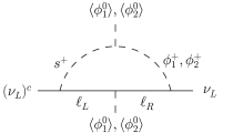
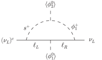
Figure 1: The loop diagram for the Majorana neutrino mass in the Zee model (left). The right diagram is a simplified one without FCNC.

In the Zee-Babu model (ZB model) ZB , Majorana neutrino masses are generated by the 2-loop diagram in Fig. 3 in which $s^{+}$ and $s^{++}$ are utilized. The scale of the neutrino mass $m_{\nu}$ can be naively given by $y_{\text{new}}^{3}\,\mu_{3}m_{\tau}^{2}/(16\pi^{2}M)^{2}$, where $y_{\text{new}}$ denotes new Yukawa coupling constant (a common value for $s^{+}$ and $s^{++}$ is assumed), the coupling constant $\mu_{3}$ (its mass-dimension is 1) is for the $s^{+}s^{+}s^{--}$ interaction, and $M$ stands for the typical mass scale of these new particles. Let’s naively take the electroweak scale $O(100)\,{\text{GeV}}$ for $\mu_{3}$ and $M$, which would enable us to discover new scalar particles experimentally in the future. A naive expectation for the size of $y_{\text{new}}$ would be the order of the Yukawa coupling constant for the $\tau$ lepton, $O(10^{-2})$. Then, the naive estimation in the ZB model gives an appropriate neutrino mass scale $m_{\nu}\sim 0.1\,{\text{eV}}$. It is worth to mention that the ZB model is viable for the model of the neutrino mass even if $m_{e}$ is simply ignored.

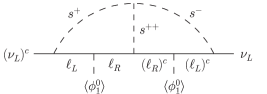
Figure 2: The loop diagram for the Majorana neutrino mass in the Zee-Babu model.

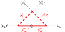
Figure 3: The loop diagram for the Majorana neutrino mass in the Ma model.

If a conserved charge is assigned only to new particles, it is easy to construct a loop diagram which involves only new particles in the loop. In addition, the lightest one among the charged particles becomes stable, and the one can be a dark matter candidate if it is electrically neutral. In the Ma model Ma:2006km as the simplest example, $\psi_{R}^{0}$ and the second ${\text{SU}}(2)_{L}$-doublet scalar field $\Phi_{2}$ are introduced such as they have the odd parity (”charge” $-1$) under an unbroken $Z_{2}$ symmetry while the standard model particles have the even parity (”charge” $1$). These $Z_{2}$-odd particles are utilized in the 1-loop diagram (Fig. 3) for Majorana neutrino masses. When $\psi_{R}^{0}$ or $\text{Re}(\phi_{2}^{0})$ or $\text{Im}(\phi_{2}^{0})$ is the lightest $Z_{2}$-odd particle, the particle can be considered as a dark matter candidate.

The first model of the radiatively generated neutrino mass with the dark matter candidate in the loop is the Krauss-Nasri-Trodden model (KNT model) Krauss:2002px . Majorana neutrino masses come from the 3-loop diagram (Fig. 4). Fermions $\psi_{R}^{0}$ and an ${\text{SU}}(2)_{L}$-singlet scalar field $s_{2}^{+}$ are introduced as $Z_{2}$-odd particles while the other singlet scalar field $s_{1}^{+}$ and the standard model particles are $Z_{2}$-even ones. The $\psi_{R}^{0}$ is the dark matter candidate if it is the lightest $Z_{2}$-odd particle. Similarly to the ZB model, $m_{e}$ can be ignored in the loop diagram.

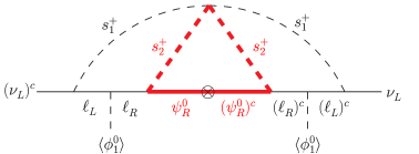
Figure 4: The loop diagram for the Majorana neutrino mass in the Krauss-Nasri-Trodden model.

The Aoki-Kanemura-Seto model (AKS model) AKS is also a 3-loop model of the Majorana neutrino mass with a dark matter candidate. Instead of $s_{1}^{+}$ in the KNT model, $s^{0}$ with the $Z_{2}$-odd parity and the second ${\text{SU}}(2)_{L}$-doublet scalar field $\Phi_{2}$ with the $Z_{2}$-even parity are utilized in the 3-loop diagram (Fig. 6). Since both of two ${\text{SU}}(2)_{L}$-doublet scalar fields are $Z_{2}$-even ones, the scalar potential in this model has the CP-violating phases which can be utilized for the electro-weak baryogenesis. Simplification with $m_{e}=0$ is not allowed, and then the Yukawa interaction of $s_{2}^{-}$ is dominated by the one with $e_{R}$.

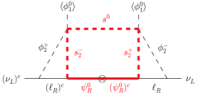
Figure 5: The loop diagram for the Majorana neutrino mass in the Aoki-Kanemura-Seto model.

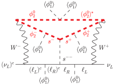
Figure 6: The loop diagram for the Majorana neutrino mass in the Gustafsson-No-Rivera model.

The 3-loop diagram (Fig. 6) in the Gustafsson-No-Rivera model (GNR model) Gustafsson:2012vj involves a dark matter candidate ($\text{Re}(\phi_{2}^{0})$ or $\text{Im}(\phi_{2}^{0})$) and the $W$ boson. The structure of the neutrino mass matrix is simply determined by a unique matrix of new Yukawa coupling constants and a known diagonal matrix of charged lepton masses. Inversely, the structure of the new Yukawa matrix is directly constrained by the neutrino oscillation data. Notice that $m_{e}$ cannot be ignored in the loop diagram in the GNR model in contrast with the cases in the Zee model and the ZB model.

Dirac masses for neutrinos can be also radiatively generated by using a softly-broken symmetry (e.g., $Z_{2}$, a global ${\text{U}}(1)$) which forbids some tree level interactions. In the Nasri-Moussa model (NM model) Nasri:2001ax  (See also Ref. Kanemura:2011jj ), $\psi_{R}^{0}$ and $s_{2}^{+}$ are introduced as $Z_{2}$-odd fields while another scalar field $s_{1}^{+}$ is a $Z_{2}$-even one. An Yukawa interaction $\overline{L}\epsilon\Phi_{1}^{\ast}\psi_{R}^{0}$ is forbidden by the $Z_{2}$ symmetry. However, the Yukawa interaction arises at the 1-loop level (Fig. 8) because the $Z_{2}$ symmetry is softly-broken by the $m_{12}^{2}s_{1}^{+}s_{2}^{-}$ term. Then, neutrinos acquire Dirac masses, and $\psi_{R}^{0}$ become the right-handed neutrinos.

Figure 7: The loop diagram for the Dirac mass of the neutrino in the Nasri-Moussa model.

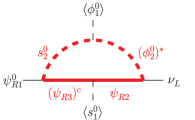
Figure 8: The loop diagram for the Dirac neutrino mass in the Gu-Sarkar model.

In the Gu-Sarkar model (GS model) Gu:2007ug , dark matter candidates are involved in the 1-loop diagram (Fig. 8) for Dirac neutrino masses. Although fermions $\psi_{R1}^{0}$ and $(\psi_{R3}^{0})^{c}$ and a complex scalar field $s_{1}^{0}$ are singlet under the gauge group of the standard model, they have a common charge of a ${\text{U}}(1)^{\prime}$ gauge symmetry which forbid Yukawa interactions $\overline{L}\epsilon\Phi_{1}^{\ast}\psi_{R1}^{0}$ at the tree level. The ${\text{U}}(1)^{\prime}$ gauge symmetry is spontaneously broken by a vacuum expectation value (VEV) of $s_{1}^{0}$. On the other hand, an unbroken $Z_{2}$ symmetry is imposed such that $\psi_{R2}^{0}$, $\psi_{R3}^{0}$, $s_{2}^{0}$, and $\Phi_{2}$ are odd under the symmetry. The conservation of the lepton number is also imposed such that $\psi_{R1}^{0}$, $\psi_{R2}^{0}$, and $(\psi_{R3}^{0})^{c}$ have a common lepton number $1$ while three new scalar fields have no lepton number; the lepton number conservation is necessary to forbids the diagram in Fig. 3 with the Majorana mass term of $\psi_{R2}^{0}$. Dirac neutrinos are made from $\nu_{L}$ and $\psi_{R1}^{0}$.

In models shown above, interactions between neutrinos and scalar fields are induced at the loop level. In contrast, the Kanemura-Sugiyama model (KS model) Kanemura:2012rj is an extension of the Higgs triplet model (HTM) Ref:HTM such that a VEV of an ${\text{SU}}(2)_{L}$-triplet scalar field $\Delta$ arises at the 1-loop level while a Yukawa interaction of Majorana neutrinos with the triplet scalar field exists at the tree level (Fig. 10). Scalar fields $s_{2}^{0}$ and $\Phi_{2}$ are introduced as $Z_{2}$-odd ones while $s_{1}^{0}$ is a $Z_{2}$-even field. A lepton number $-1$ is assigned to $\Phi_{2}$ and $s_{1}^{0}$, and a VEV of $s_{1}^{0}$ spontaneously breaks the lepton number conservation without breaking the $Z_{2}$ symmetry which stabilizes a dark matter candidate. The direct relation between the Yukawa matrix with $\Delta$ and the neutrino mass matrix remain the same as the one in the HTM.

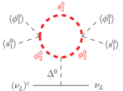
Figure 9: The loop diagram for the VEV of an ${\text{SU}}(2)_{L}$-triplet scalar field in the Kanemura-Sugiyama model.

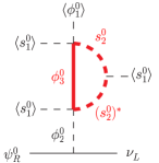
Figure 10: The loop diagram for the VEV of an ${\text{SU}}(2)_{L}$-doublet scalar field which couples only with the neutrino in the Kanemura-Matsui-Sugiyama model.

The Kanemura-Matsui-Sugiyama model (KMS model) Kanemura:2013qva is an extension of a version of the two Higgs doublet model where the second ${\text{SU}}(2)_{L}$-doublet scalar field $\Phi_{2}$ has the Yukawa interaction only with neutrinos ($\nu$THDM) Ref:nuTHDM-1 . The VEV of $\Phi_{2}$ in the KMS model is obtained via a 1-loop diagram in Fig. 10. A global ${\text{U}}(1)$ symmetry is imposed such that charges of $\psi_{R}^{0}$, $s_{1}^{0}$, and $\Phi_{2}$ are $3$, $1$, and $3$, respectively. Fields which exist in the standard model have no charge for the global ${\text{U}}(1)$ symmetry, and Yukawa interaction between $\psi_{R}^{0}$ and $\Phi_{1}$ is forbidden. The ${\text{U}}(1)$ symmetry is spontaneously broken by a VEV of $s_{1}^{0}$. On the other hand, $s_{2}^{0}$ and $\Phi_{3}$ have fractional charges $1/2$ and $3/2$, respectively; there appears an accidental unbroken global ${\text{U}}(1)_{D}$ symmetry under which $s_{2}^{0}$ and $\Phi_{3}$ has the same charge, which stabilizes a dark matter candidate.

III Phenomenology

For the lepton flavor violation in charged lepton decays, it would be naively expected that three-body decays $\ell\to\overline{\ell}_{1}\ell_{2}\ell_{3}$ are rarer than two-body decays $\ell\to\ell^{\prime}\gamma$. However, $\ell\to\overline{\ell}_{1}\ell_{2}\ell_{3}$ can be caused at the tree level while $\ell\to\ell^{\prime}\gamma$ are always given in the loop level. Such tree level $\ell\to\overline{\ell}_{1}\ell_{2}\ell_{3}$ are given by the FCNC in the Zee model or mediated by a doubly-charged scalar particle which exists in the ZB, the GNR, and the KS models; $\tau\to\overline{e}\mu\mu$ is dominant for a benchmark point in the GNR model Gustafsson:2012vj , and the KS model favors $\tau\to\overline{\mu}\mu\mu$, $\tau\to\overline{\mu}\mu e$, and $\tau\to\overline{\mu}ee$ (See e.g., Ref. Akeroyd:2009nu for the Higgs triplet model). If some $\ell\to\overline{\ell}_{1}\ell_{2}\ell_{3}$ processes are observed (especially, in the case without $\ell\to\ell^{\prime}\gamma$ signal), these models would be supported.

A doubly-charged scalar particle can decay into a pair of same-signed charged leptons, $H^{--}\to\ell\ell^{\prime}$. Such a particle is involved in the ZB, the GNR, and the KS models. In the ZB model, it is naively expected that decay branching ratios for $s^{--}\to\mu_{R}\tau_{R}$ and $\tau_{R}\tau_{R}$ are suppressed by $(m_{\mu}/m_{\tau})^{2}$ and $(m_{\mu}/m_{\tau})^{4}$, respectively, in comparison with the ratio for $s^{--}\to\mu_{R}\mu_{R}$ (See e.g., Ref, AristizabalSierra:2006gb ). Thus, $s^{--}\to\tau_{R}\tau_{R}$ is not expected to be observed in the ZB model. Similarly to the ZB model, a matrix $h_{\ell\ell^{\prime}}^{\text{(GNR)}}$ of Yukawa coupling constants for $s^{--}$ in the GNR model has a very hierarchical structures because of the charged lepton masses in the loop diagram (Fig. 6), $h_{\ell\ell^{\prime}}^{\text{(GNR)}}\propto(m_{\nu})_{\ell\ell^{\prime}}/(m_{\ell}m_{\ell^{\prime}})$. Therefore, the leptonic decay of $s^{--}$ prefers to involve an electron. A decay $s^{--}\to e_{R}\tau_{R}$ is dominant for a scenario where both of $|(m_{\nu})_{ee}|$ and $|(m_{\nu})_{e\mu}|$ are assumed to be negligible, and a benchmark values of parameters for the scenario is shown in Ref. Gustafsson:2012vj . In the KS model, predictions for $\Delta^{--}\to\ell_{L}\ell_{L}^{\prime}$ are the same as those in the Higgs triplet model (See e.g., Ref. Akeroyd:2007zv ).

Singly-charged scalar particles are involved in all models in Table 1. Mixings between scalar particles are ignored in most of discussion below for simplicity. Since we do not observe flavors of neutrinos in $H^{-}$ decays, let us define branching ratios ${\text{BR}}(H^{-}\to\ell\nu)\equiv\sum_{\ell^{\prime}}{\text{BR}}(H^{-}\to\ell\nu_{\ell^{\prime}})$. Flavor structures of ${\text{BR}}(\phi_{2}^{-}\to\ell_{R}\overline{\nu_{L}})$ in the Zee model and ${\text{BR}}(s_{2}^{-}\to\ell_{R}\psi_{R}^{0})$ in the NM model are arbitrary. For an antisymmetric matrix $f_{\ell\ell^{\prime}}^{\text{(ZM)}}$ of Yukawa coupling constants for $s^{-}$ in the Zee model, a simplification with $m_{e}=m_{\mu}=0$ results in $|f_{\mu\tau}^{\text{(ZM)}}|^{2}\ll|f_{e\tau}^{\text{(ZM)}}|^{2}$. Then, the Zee model predicts ${\text{BR}}(s^{-}\to e_{L}\nu_{L}):({\text{BR}}(s^{-}\to\mu_{L}\nu_{L})+{\text{BR}}(s^{-}\to\tau_{L}\nu_{L}))\simeq 1:1$. Decay branching ratios ${\text{BR}}(s^{-}\to\ell_{L}\nu_{L})$ in the ZB model for Majorana mass terms and ${\text{BR}}(s_{1}^{-}\to\ell_{L}\nu_{L})$ in the NM model for Dirac mass terms have a common flavor structure. These models predict ${\text{BR}}(H^{-}\to e_{L}\nu_{L}):{\text{BR}}(H^{-}\to\mu_{L}\nu_{L}):{\text{BR}}(H^{-}\to\tau_{L}\nu_{L})\simeq 2:5:5$ for the so-called normal mass ordering ($m_{1}<m_{3}$ where $m_{i}$ denote neutrino masses) and $2:1:1$ for the so-called inverted mass ordering ($m_{3}<m_{1})$. In the AKS model, the second ${\text{SU}}(2)_{L}$-doublet field couples only with leptons, and its VEV gives charged lepton masses. Therefore, the leptonic decay of $\phi_{2}^{-}$ is dominated by the decay into $\tau_{R}$.

There exists a singly-charged scalar particle from an ${\text{SU}}(2)_{L}$-doublet field which is $Z_{2}$-odd (or charged under a global ${\text{U}}(1)$) in the Ma, the GNR, the KS, the GS, and the KMS models. In the GNR, the KS, and the KMS models, $\phi_{2}^{-}$ dominantly decays into $W^{-}$. Then, the decay of the $\phi_{2}^{-}$ gives charged leptons with the equal ratio $e:\mu:\tau=1:1:1$. This is also the case in the Ma and the GS models if the weak decay of $\phi_{2}^{-}$ is dominant. If $\phi_{2}^{-}\to\ell_{L}\overline{\psi_{R}^{0}}$ is dominant in these two models, we do not have clear predictions on the flavor structure.

The KNT, the AKS, and the GNR models contain a singly-charged ${\text{SU}}(2)_{L}$-singlet scalar particle with the $Z_{2}$-odd parity. In the KNT model, the Yukawa interaction of $s_{2}^{-}$ with $\tau_{R}$ would be suppressed by $m_{\mu}/m_{\tau}$ in comparison with that with $\mu_{R}$ (See e.g., Ref. Cheung:2004xm for benchmark values of parameters) similarly to the expected hierarchy in Yukawa coupling constants for $s^{--}$ in the ZB model. Therefore, branching ratio for $s_{2}^{-}\to\tau_{R}\psi_{R}^{0}$ becomes too tiny to be measured. In the AKS model, $s^{-}$ can decay as $s^{-}\to\phi_{2}^{-}s^{0}$ followed by the decay of $\phi_{2}^{-}$ into $\tau_{R}$ for parameter sets in Ref. AKS . If $s^{-}\to\ell_{R}\psi_{R}^{0}$ is kinematically possible, $s^{-}$ dominantly decays into an electron. The $s^{-}$ in the GNR model decays into $W$ through the mixing between $s^{-}$ and $\phi_{2}^{-}$, and the ratio of produced charged leptons is the same as that for the $\phi_{2}^{-}$ decay, $e:\mu:\tau=1:1:1$. Prediction about leptonic decays of singly-charged Higgs bosons in the KS and KMS models are the same as those in the HTM model and the $\nu$THDM model, respectively, because there is no extension for Yukawa interactions. Figure 11 (taken from Ref. Perez:2008ha ) shows the prediction in the HTM, which is also the one in the $\nu$THDM Ref:nuTHDM-2 ; the Fig. 11 can be used for both of the KS and KMS models.

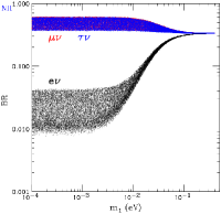
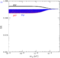
Figure 11: Leptonic decays of a charged Higgs boson in the HTM for $m_{1}<m_{3}$ (left) and $m_{3}<m_{1}$ (right), where $m_{i}$ are neutrino mass eigenstates. These plots are taken from Ref. Perez:2008ha , which are the same in the KS and the KMS models.

III.1 Summary

New Higgs bosons are introduced in radiative neutrino mass models where neutrino masses are generated at the loop level, and it is not necessary for these bosons to be very heavy. Since their Yukawa interactions relate to the structure of neutrino mass matrix which is constrained by the neutirno oscillation data, we have predictions about $\ell\to\overline{\ell}_{1}\ell_{2}\ell_{3}$ and leptonic decays of singly and doubly-charged Higgs bosons. Such predictions can be used to test these models. We hope that some signal of such processes are observed in near future, which would drive us to meet again in Toyama.

- (1) G. Aad et al. [ATLAS Collaboration], Phys. Lett. B 716, 1 (2012); S. Chatrchyan et al. [CMS Collaboration], Phys. Lett. B 716, 30 (2012); G. Aad et al. [ATLAS and CMS Collaborations], arXiv:1503.07589 [hep-ex].
- (2) The ATLAS collaboration, ATLAS-CONF-2015-007, ATLAS-COM-CONF-2015-011; V. Khachatryan et al. [CMS Collaboration], arXiv:1412.8662 [hep-ex].
- (3) P. Minkowski, Phys. Lett. B 67, 421 (1977); T. Yanagida, Conf. Proc. C 7902131, 95 (1979); Prog. Theor. Phys. 64, 1103 (1980); M. Gell-Mann, P. Ramond and R. Slansky, Conf. Proc. C 790927, 315 (1979); R. N. Mohapatra and G. Senjanovic, Phys. Rev. Lett. 44, 912 (1980).
- (4) A. Zee, Phys. Lett. B 93, 389 (1980) [Phys. Lett. B 95, 461 (1980)].
- (5) A. Zee, Nucl. Phys. B 264, 99 (1986); K. S. Babu, Phys. Lett. B 203, 132 (1988).
- (6) E. Ma, Phys. Rev. D 73, 077301 (2006).
- (7) L. M. Krauss, S. Nasri and M. Trodden, Phys. Rev. D 67, 085002 (2003).
- (8) M. Aoki, S. Kanemura and O. Seto, Phys. Rev. Lett. 102, 051805 (2009); Phys. Rev. D 80, 033007 (2009).
- (9) M. Gustafsson, J. M. No and M. A. Rivera, Phys. Rev. Lett. 110, no. 21, 211802 (2013) [Phys. Rev. Lett. 112, no. 25, 259902 (2014)].
- (10) S. Kanemura and H. Sugiyama, Phys. Rev. D 86, 073006 (2012).
- (11) S. Nasri and S. Moussa, Mod. Phys. Lett. A 17, 771 (2002).
- (12) P. H. Gu and U. Sarkar, Phys. Rev. D 77, 105031 (2008).
- (13) S. Kanemura, T. Matsui and H. Sugiyama, Phys. Lett. B 727, 151 (2013).
- (14) L. Wolfenstein, Nucl. Phys. B 175, 93 (1980).
- (15) X. G. He, Eur. Phys. J. C 34, 371 (2004).
- (16) X. G. He and S. K. Majee, JHEP 1203, 023 (2012).
- (17) S. Kanemura, T. Nabeshima and H. Sugiyama, Phys. Lett. B 703, 66 (2011).
- (18) W. Konetschny and W. Kummer, Phys. Lett. B 70, 433 (1977); M. Magg and C. Wetterich, Phys. Lett. B 94, 61 (1980); T. P. Cheng and L. F. Li, Phys. Rev. D 22, 2860 (1980); G. Lazarides, Q. Shafi and C. Wetterich, Nucl. Phys. B 181, 287 (1981).
- (19) F. Wang, W. Wang and J. M. Yang, Europhys. Lett. 76, 388 (2006); S. Gabriel and S. Nandi, Phys. Lett. B 655, 141 (2007).
- (20) A. G. Akeroyd, M. Aoki and H. Sugiyama, Phys. Rev. D 79, 113010 (2009).
- (21) D. Aristizabal Sierra and M. Hirsch, JHEP 0612, 052 (2006).
- (22) A. G. Akeroyd, M. Aoki and H. Sugiyama, Phys. Rev. D 77, 075010 (2008).
- (23) K. Cheung and O. Seto, Phys. Rev. D 69, 113009 (2004).
- (24) P. Fileviez Perez, T. Han, G. -y. Huang, T. Li and K. Wang, Phys. Rev. D 78, 015018 (2008).
- (25) S. M. Davidson and H. E. Logan, Phys. Rev. D 80, 095008 (2009).