String Formation Beyond Leading Colour
Jesper R. Christiansen, Peter Z. Skands
: Department of Astronomy and Theoretical Physics, Lund University, Sölvegatan 14, Lund, Sweden
: Theoretical Physics, CERN, CH-1211, Geneva 23, Switzerland
: School of Physics and Astronomy, Monash University, VIC-3800, Australia
Abstract
We present a new model for the hadronisation of multi-parton systems, in which colour correlations beyond leading are allowed to influence the formation of confining potentials (strings). The multiplet structure of is combined with a minimisation of the string potential energy, to decide between which partons strings should form, allowing also for “baryonic” configurations (e.g., two colours can combine coherently to form an anticolour). In collisions, modifications to the leading-colour picture are small, suppressed by both colour and kinematics factors. But in collisions, multi-parton interactions increase the number of possible subleading connections, counteracting their naive suppression. Moreover, those that reduce the overall string lengths are kinematically favoured. The model, which we have implemented in the PYTHIA 8 generator, is capable of reaching agreement not only with the important distribution but also with measured rates (and ratios) of kaons and hyperons, in both and collisions. Nonetheless, the shape of their spectra remains challenging to explain.
1 Introduction
The description of hadronic final states at high-energy colliders involves a complicated cocktail of physics effects, dominated by QCD Dissertori:2003pj ; Skands:2012ts ; Buckley:2011ms . For the calculation of inclusive hard-scattering cross sections, factorisation allows most of the complicated long-distance physics to be represented in the form of universal parton distribution functions (PDFs) Ball:2012wy , while the short-distance parts can be calculated perturbatively. Perturbative aspects, such as hard-process matrix elements, parton showers, and decay (chains) of short-lived resonances, are generally coming under increasingly good control, due to a combination of advances: better amplitude calculations (including better automation and better interfaces Boos:2001cv ; Alwall:2006yp ; vanHameren:2009dr ; Cascioli:2011va ; Alwall:2011uj ; Alioli:2013nda ; Cullen:2014yla ; Alwall:2014hca ), better parton-shower algorithms (e.g. ones based on QCD dipoles Gustafson:1987rq ; Sjostrand:2004ef ; Nagy:2005aa ; Giele:2007di ; Dinsdale:2007mf ; Schumann:2007mg ; Platzer:2009jq ), and better techniques for how to combine them (matching and merging, see Buckley:2011ms ; Hamilton:2012np ; Lonnblad:2012ix ; Hartgring:2013jma ; Alwall:2014hca and references therein). These successes build on an extensive prior experience with perturbative approximations to QCD at both fixed and infinite order, and the tractable nature of the perturbative expansions themselves.
To describe the full (exclusive) event structure, however, several additional soft-physics effects must be accounted for, such as hadronisation, multiple parton interactions (MPI), Bose-Einstein correlation effects, and beam remnants. These are connected with the rich structure of QCD beyond perturbation theory and are vital, each in their own way, to the understanding of issues such as underlying-event/pileup effects on isolation and accurate jet calibrations, and the interpretation of identified-particle rates and spectra.
For these aspects, explicit calculations can only be performed in the context of simplified phenomenological models, constructed so as to capture the essential features of full (nonperturbative) QCD. An example relevant to this paper is the Lund string model of hadronisation Andersson:1998tv ; Andersson:1983ia , whose cornerstone is the observation that the static QCD potential between a quark and an antiquark in an overall colour-singlet state grows linearly with the distance between them, for distances larger than about 0.5 fm Bali:1992ab . This is interpreted as a consequence of the gluon field between the charges forming a high-tension “string” (with tension ), which subsequently fragments into hadrons.
While the details of the string-breaking process may be complicated (the Lund model invokes quantum tunnelling to describe this aspect Andersson:1998tv ), the first question that any hadronisation model needs to address is therefore simply: between which partons do confining potentials arise? In string-based models, this is equivalent to answering the question between which partons string pieces should be formed. Traditionally, Monte Carlo event generators make use of the leading-colour (LC) approximation to trace the colour flow on an event-by-event basis (see Buckley:2011ms ; pdg2012 ), leading to partonic final states in which each quark is colour-connected to a single (unique) other parton in the event (equivalent to a leading-colour QCD dipole Gustafson:1986db ). Gluons are represented as carrying both a colour and an anticolour charge, and are hence each connected to two other partons. At the level of strings, this is interpreted as gluons forming transverse “kinks” on strings whose endpoints are quarks and antiquarks Andersson:1998tv . Studies at colliders show this to be a quite reasonable approximation in that environment, and the traditional Lund string model, implemented in PYTHIA Sjostrand:2006za ; Sjostrand:2007gs ; Sjostrand:2014zea , is capable of delivering a good description of the vast majority of collider data (for recent studies, see, e.g., Buckley:2009bj ; Firdous:2013noa ; Fischer:2014bja ; Skands:2014pea ).
The question of colour reconnections (CR) — broadly, whether other string topologies than the LC one could lead to non-negligible corrections with respect to the LC picture — was studied at LEP Abbiendi:2003ri ; Achard:2003pe ; Achard:2003ik ; Siebel:2005uw ; Abbiendi:2005es ; Schael:2006ns ; Abdallah:2006uq ; Schael:2006mz , chiefly in the context of CR uncertainties on mass determinations in Sjostrand:1993hi , with conclusion that excluded the very aggressive models and disfavoured the no CR scenario at 2.8 standard deviation Schael:2013ita . The uncertainty on the mass from this source ended up at , corresponding to about 0.05%.
There are strong physical reasons to think that CR effects should be highly suppressed at LEP, however. Firstly, there is a “trivial” parametric suppression of beyond-LC effects of order . Secondly, the two decay systems are separate colour-singlet systems, with a space-time separation of order of the inverse width, . This separation implies that interference effects between the two systems should be highly suppressed for wavelengths shorter than , i.e., there can be essentially no perturbative cross-talk between them. This line of argument motivated the phrasing of CR models that operate only at the non-perturbative level as the most physically reasonable Sjostrand:1993hi , an observation that we shall also adhere to in the present work. Thirdly, the QCD coherence of perturbative parton cascades implies that, inside each (or ) decay system, angles of successive QCD emissions tend to be ordered from large to small Marchesini:1983bm , so that there is very little space-time overlap between the QCD dipoles inside each system. This means that, even if one were to allow to set up confining potentials between non-LC-connected partons, these would tend to correspond to larger opening angles and therefore they would have a higher total potential energy (longer strings) than the equivalent LC ones. The LC topology should therefore also be dynamically favoured over any possible non-LC ones. All these factors contribute to an expectation of quite small effects, at least in the context of collisions.
Moving to collisions (and using as a shorthand to for any generic hadron-hadron collision, including in particular also ones), the situation changes dramatically. Trivially, one must now include coloured initial-state partons, with associated coloured beam remnants. But more importantly, the modern understanding of the underlying event (UE) and of soft-inclusive (minimum-bias/pileup) physics in general, especially at high particle multiplicities, is that they are dominated by contributions from multiple parton interactions (MPI) Sjostrand:1987su . In a event that contains several MPI systems, there is a non-negligible possibility of phase-space overlaps between final states from different MPI systems. Moreover, since the MPI scattering centres must all reside within the proton radius, which is of the same order as the transverse size of QCD strings, the initial-state (beam) jets will all “sit” right on top of each other, a situation which should affect the fragmentation especially at high rapidities. Finally, unlike the case for angular-ordered partons inside a jet, there is no perturbative principle that predisposes colour-connected partons from different MPI or beam-remnant systems to have small opening angles; indeed a recent study Gieseke:2012ft found that such “inter-MPI/remnant” invariant masses (denoted -type and -type in Gieseke:2012ft ) tend to be among the largest in the events, corresponding to a high potential energy in a string context, and hence with the most to gain from potential reconnections. For these reasons, we expect qualitatively larger effects in collisions.
There are also tantalising hints from hadron-collider data that nontrivial physics effects are present at the hadronisation stage in collisions. The most important such clue is furnished by the dependence of the average (charged) particle on the particle multiplicity, . Measurements of this quantity in minimum-bias events, first made at the ISR Breakstone:1983up and since by UA1 Albajar:1989an , CDF Acosta:2001rm ; Aaltonen:2009ne and the LHC experiments Khachatryan:2010nk ; Aad:2010ac ; Abelev:2013bla , reveal that grows with , as can be seen in the plots in fig. 1 (from mcplots.cern.ch Karneyeu:2013aha ).

This cannot be accounted for by independently hadronising MPI systems, for which the expectation would be that should be almost flat, as is also illustrated by the “no CR” curves in fig. 1. (If each MPI hadronises independently, then per-particle quantities such as should be independent of the number of MPI, which is correlated with Sjostrand:1987su .) The observation that increases with therefore strongly suggests that some form of collective hadronisation phenomenon is at play, correlating partons from different MPI systems.
Given these arguments, and the realisation Skands:2007zg that precision kinematic extractions of the top quark mass at hadron colliders (see e.g., Aaltonen:2012va ; Chatrchyan:2012cz ; Aaltonen:2013wca ; Chatrchyan:2013xza ; ATLAS:2014wva ; Abazov:2014dpa ; Aad:2015nba for experimental methods and Juste:2013dsa for a recent phenomenology review) can be significantly affected by colour reconnections111For completeness we note that, similarly to above, much smaller effects are expected in environments Khoze:1994fu ; Khoze:1999up ., several toy models have appeared Rathsman:1998tp ; Sandhoff:2005jh ; Buttar:2006zd ; Skands:2007zg ; Gieseke:2012ft ; Argyropoulos:2014zoa , relying mainly on potential-energy minimisation arguments to reconfigure the partonic colour connections for hadronisation. Although these models have had some success in describing the distribution (as e.g., in fig. 1), the lack of rigorous underpinnings have implied that large uncertainties remain, which still contribute about a 500 MeV uncertainty on the hadronic top mass extraction Juste:2013dsa ; ATLAS:2014wva ; Argyropoulos:2014zoa . In this paper, we take a first step towards creating a more realistic model, combining the earlier string-length minimisation arguments with selection rules based on the colour algebra of . Our treatment amounts to taking the LC connections produced by the shower as a starting point, complemented by an -weighted randomization over the set of possible subleading topologies that would have been present in a full-colour treatment. The missing colour information should thereby be restored, at least in a statistical sense.
An alternative line of argument, pursued in particular in the EPOS model Pierog:2013ria , invokes the notion of hydrodynamic collective flow to explain the distribution (as well as the so-called CMS “ridge effect” Khachatryan:2010gv ; Werner:2010ss and a host of other observables Pierog:2013ria ). Certainly, the presence of hydro effects in is a hypothesis that, if confirmed, would have far-reaching consequences, and it will be an important task for future experimental and phenomenological studies to find ways of disentangling CR effects from hydro ones. In this context, our paper should therefore also be viewed as an attempt to see how far one can get without postulating genuine (pressure-driven) collective-flow effects in . Within this context, it is important to note that CR can mimic flow effects to some extent, via the creation of boosted strings Ortiz:2013yxa . Alternatively, it is possible that the effective string tension could be rising, as in the idea of colour ropes Andersson:1991er , with recent work along these lines reported on by the Lund group Bierlich:2014xba . Finally, we note that non-hydro rescattering has also been proposed Corke:2009tk as a potential mechanism contributing to the rise of , though the explicit model of parton-parton rescattering effects presented in Corke:2009tk found only very small effects. The possibility of Boltzmann-like elastic (or even inelastic) final-state hadron-hadron rescattering is still open. As usual, nature’s solution is likely to involve an interplay of effects at different levels. Nevertheless, before exploring further effects at the hadron level, we believe it makes good sense to first examine the hadronisation process itself, which is the topic of this work.
Finally, we note that colour flows beyond LC have also been invoked in the context of formation Fritzsch:1977ay ; Ali:1978kn ; Fritzsch:1979zt ; Eriksson:2008tm , and as a potential mechanism to generate diffractive topologies in and collisions Buchmuller:1995qa ; Edin:1995gi .
In section 2, we briefly recapitulate the treatment of colour space for the existing MPI models in PYTHIA, and present the new model that we have developed, combining the minimisation of the string potential with the multiplet structure of QCD. In section 3, we constrain the resulting free model parameters on a selection of both and data, discussing the physics consequences of the new colour-space treatment as we go along. In section 4, we consider implications for precision extractions of the top quark mass at hadron colliders. Finally, in section 5, we summarise and give an outlook.
2 The Model
In this section, we present the colour-space model that we have developed, which allows strings to form not only between LC-connected partons, but also between specific non-LC-connected ones, following combination rules that approximate the multiplet structure of full-colour QCD. We begin with a brief summary of the current modelling, in section 2.1. We then turn to a general discussion of coherence effects beyond leading in section 2.2. Finally, in section 2.3, we present the detailed implementation of the new model.
We emphasise that there is a conceptual difference between colour-space ambiguities, such as those explored in this work, and physical colour reconnections. The subleading-colour effects we discuss here arise naturally in “full-colour” and do not involve any physical exchange of colour or momentum (although explicit algorithms may of course still employ an iterative-reconnection scheme to find the potential-energy minimum). Strictly speaking, the term colour reconnections should be reserved to describe effects related to dynamical reconfigurations of the colour/string space that involve explicit exchange of colours and momentum, via perturbative gluon exchanges or non-perturbative string interactions. Effects of this type are not explored directly in this work, instead we refer the interested reader to the SK string-interaction models presented in Sjostrand:1993hi ; Khoze:1994fu ; Khoze:1999up . Somewhat sloppily, we follow the entrenched convention in the field and use the acronym “CR” for effects of either kind here.
2.1 Existing MPI Models and Colour Space
In a naive LC picture, each MPI scattering system is viewed as separate and distinct from all other systems in colour space. The very simplest colour-space options in the old PYTHIA 6 MPI model Sjostrand:1987su and the first HERWIG (and HERWIG++) MPI models Butterworth:1996zw ; Gieseke:2010zz go a step further, representing each MPI final state as two quarks (or gluons), colour-connected directly to each other, i.e., treating each MPI system as a separate hadronising colour-singlet system. However, this ignores that the incoming partons are coloured, and hence that the total colour charge of each MPI scattering system is in general non-zero. These particular models therefore violate colour conservation and are unphysical.
To be LC-correct one must take into account that each MPI-initiator parton should cause one or two strings to be stretched to its remnant (one for quarks, two for gluons). This conserves colour, but still has the implication that no strings would be stretched between different MPI systems. This situation is illustrated in fig. 2(a).
remnantcolora {fmfgraph*}(52,22) \fmfstraight\fmftopmpi1l,mpi1c,mpi1r,mpi2l,mpi2c,mpi2r,mpi3l,mpi3c,mpi3r \fmfbottombr1l,br1c,br1r,br2l,br2c,br2r,br3l,br3c,br3r \fmfvd.shape=circle,d.fill=empty,label.dist=0,d.siz=32,label=MPI 1mpi1c \fmfvd.shape=circle,d.fill=empty,label.dist=0,d.siz=32,label=MPI 2mpi2c \fmfvd.shape=circle,d.fill=empty,label.dist=0,d.siz=32,label=MPI 3mpi3c \fmfdbl_plain,label=Hadron Remnantbr1l,br3r \fmfgluonbr1c,mpi1c \fmfgluonbr2c,mpi2c \fmfgluonbr3c,mpi3c \fmffreeze\fmfiplain,fore=redvpath (__br1c,__mpi1c) shifted (thick*(-3,1)) \fmfiplain,fore=redvpath (__br1c,__mpi1c) shifted (thick*(5,1)) \fmfiplain,fore=redvpath (__br2c,__mpi2c) shifted (thick*(-3,1)) \fmfiplain,fore=redvpath (__br2c,__mpi2c) shifted (thick*(5,1)) \fmfiplain,fore=redvpath (__br3c,__mpi3c) shifted (thick*(-3,1)) \fmfiplain,fore=redvpath (__br3c,__mpi3c) shifted (thick*(5,1))
remnantcolorb {fmfgraph*}(52,22) \fmfstraight\fmftopmpi1l,mpi1c,mpi1r,mpi2l,mpi2c,mpi2r,mpi3l,mpi3c,mpi3r \fmfbottombr1l,br1c,br1r,br2l,br2c,br2r,br3l,br3c,br3r \fmfvd.shape=circle,d.fill=empty,label.dist=0,d.siz=32,label=MPI 1mpi1c \fmfvd.shape=circle,d.fill=empty,label.dist=0,d.siz=32,label=MPI 2mpi2c \fmfvd.shape=circle,d.fill=empty,label.dist=0,d.siz=32,label=MPI 3mpi3c \fmfdbl_plain,label=Hadron Remnantbr1l,br3r \fmfgluonbr1c,mpi1c \fmfgluonbr2c,mpi2c \fmfgluonbr3c,mpi3c \fmffreeze\fmfphantombr1r,br2c \fmfphantombr2r,br3c \fmfiplain,fore=redvpath (__br1c,__mpi1c) shifted (thick*(-3,1)) \fmfiplain,fore=redvpath (__br1c,__mpi1c) shifted (thick*(5,3)) \fmfiplain,fore=redvpath (__br2c,__mpi2c) shifted (thick*(-3,3)) \fmfiplain,fore=redvpath (__br2c,__mpi2c) shifted (thick*(5,3)) \fmfiplain,fore=redvpath (__br3c,__mpi3c) shifted (thick*(-3,3)) \fmfiplain,fore=redvpath (__br3c,__mpi3c) shifted (thick*(5,1)) \fmfiplain,fore=redvpath (__br1r,__br2c) shifted (thick*(-3.5,3)) \fmfiplain,fore=redvpath (__br2r,__br3c) shifted (thick*(-3.5,3)) \fmffreeze
Physically, this can lead to arbitrarily many strings being stretched across the central rapidity region, one or two for each MPI (corresponding to adding their total colour chargers together as scalar quantities, rather than as vectors).
However, already in the context of earlier works Sjostrand:1987su ; Sjostrand:2004pf , it was noted that even this picture cannot be quite physically correct. Since all the MPI initiators on each side are extracted from one and the same (colour-singlet) beam particle, and since they are extracted at a rather low scale of order the perturbative evolution cutoff , there is presumably some overlap and accompanying saturation effects, implying that they are not completely independent. Not knowing the exact form of the correlations, a pragmatic solution is to minimise the total colour charge of the remnant (and hence the number of strings stretched to it), by allowing the different MPI systems to be colour-connected to each other along a “chain” in colour space, as illustrated in fig. 2(b). Variations of this are used in the current forms of both the PYTHIA Sjostrand:1987su ; Sjostrand:2004pf and HERWIG++ Gieseke:2012ft MPI models, reducing the number of strings/clusters especially in the remnant-fragmentation region at high rapidities. It is, however, still fundamentally ambiguous exactly which systems to connect and how. In the example of fig. 2, it is arbitrary that it happens to be the colour of MPI 1 and the anticolour of MPI 3 which end up connected to the remnant. For a more detailed discussion of this aspect, see e.g. Sjostrand:2004pf . An interesting physics point is that, in this picture, the particle production at very forward rapidities is controlled essentially by how large one allows the colour charge of the remnant to become, which in turn depends on the number of MPI and their mutual colour correlations. This could presumably be revealed by studies correlating the particle production in the central region (sensitive to the number of MPI) with that in the forward region (sensitive to the total charge of the remnant).
In the absence of any further CR effects, the relationship between the number of MPI and the average particle multiplicity at central rapidities is still approximately linear. Consequently, the per-particle spectra in high-multiplicity events (with many MPI) are similar to those in (non-diffractive) low-multiplicity events (with few MPI)222For very low multiplicities, well-understood bias effects cause the average particle to increase (if the event is required to contain only one particle, then that particle must be carrying all the scattered energy), while for high multiplicities, the contribution from hard-jet fragmentation also generates slightly harder spectra.. This is what leads to the simple expectation of the flat spectrum exhibited by the “no CR” curves that were shown in fig. 1 in the previous section. However, as was also remarked on there, the experimental data convincingly rule out such a constant behaviour. This observation is the main reason additional non-trivial final-state CR effects have been included in both HERWIG++ and PYTHIA.
In the original (non-interleaved) MPI model in PYTHIA 6 Sjostrand:1987su ; Sjostrand:2006za , the parameters PARP(85) and PARP(86) allowed to force a fraction of the MPI final states to be two gluons colour-connected to their nearest neighbours in momentum space. The physical picture was that the hardest interaction built up a “skeleton” of string pieces, onto which a fraction of the gluons from MPI were grafted (by brute force) in the places where they caused the least amount of change of string length. This effectively minimised the increase in string length from those gluons. An important factor contributing to the revival of the question of CR in hadron collisions was the tuning studies of this model, carried out by Rick Field on underlying-event and minimum-bias data from the CDF experiment at the Tevatron Abe:1988yu ; Acosta:2001rm ; Affolder:2001xt . His resulting “Tune A” and related tunes Field:2002vt ; Field:2005sa were the first to give good fits to the available data at the time, but the surprising conclusion was that in order to do so this “colour-space grafting” had to be done nearly all the time.
An alternative set of CR models, which relied on physical analogies with overlapping strings in superconductors, were developed only in the context of collisions Sjostrand:1993hi ; Khoze:1994fu ; Khoze:1999up , chiefly with the aim of studying potential CR uncertainties on the mass, see Sjostrand:2013cya and references therein. As far as we are aware, this class of models has not yet been applied in the context of the more complex environment of hadron-hadron collisions.
In the new (interleaved) MPI model in PYTHIA 6 Sjostrand:2004ef ; Sjostrand:2006za , showers and MPI were carried out in parallel, with physical colour flows. This was too complicated to handle with the old CR model. A new “colour annealing” CR scenario was developed Sandhoff:2005jh ; Skands:2007zg ; Wicke:2008iz which, after the shower evolution had finished, allowed for a fraction of partons to “forget” their LC colour connections, with new ones determined based on the string area law (shorter strings are preferred), following a simplified annealing-like algorithm, in a similar spirit to an earlier model by Rathsman, called the “Generalized Area-Law” (GAL) model Rathsman:1998tp . The fraction of partons that forgot their LC colour connections was assumed to grow with the number of MPI, with a per-MPI probability given by the parameter PARP(78). A further parameter, PARP(77), allowed to suppress the reconnection probability for fast-moving partons. Although still intended as a toy model, the new colour-annealing models obtained good agreement with the Tevatron minimum-bias and underlying-event data, e.g. in the form of the Perugia family of tunes Skands:2009zm ; Skands:2010ak . The most recent incarnations, the Perugia 2011 and 2012 tunes, also included LHC data and were among the main reference tunes used during Run 1 of the LHC Skands:2010ak . However, a study comparing independent MPI+CR tunings at different collider energies revealed different preferred CR parameter values at different CM energies Schulz:2011qy , implying that the modelling of this aspect, or at least its energy dependence, was still inadequate.
In PYTHIA 8, the default MPI colour-space treatment is similar to that of the original PYTHIA 6 model, although starting out from a more detailed modelling of the colour flow in each MPI. With a certain probability, controlled by the parameter ColourReconnection:range, all the gluons of each lower- interaction can be inserted onto the colour-flow dipoles of a higher- one, in such a way as to minimise the total string length Argyropoulos:2014zoa . The effects of this model was already illustrated in fig. 1. A set of alternative CR scenarios was also presented in Argyropoulos:2014zoa , but were still mostly intended as toy models in the context of estimating uncertainties on the top-quark mass.
Finally, in the most recent developments of the HERWIG++ MPI model, an explicit scenario for colour reconnections has likewise been introduced Gieseke:2012ft , based on a simulated-annealing algorithm that minimises (sums of) cluster masses. In the context of the cluster hadronisation model Webber:1983if , the minimisation of cluster masses fulfils a similar function as the minimisation of string lengths above. The two minimisations differ in that the string length measure is closely related to the product of the invariant masses rather than the sum used in the cluster model. The main model parameter is the probability to accept a favourable reconnection, . The study in Gieseke:2012ft emphasised in particular that the largest pre-reconnection cluster masses are spanned between hard partons and the remnants (denoted -type clusters), with inter-MPI ones (spanned directly between partons from different MPI systems and denoted -type) having the second-largest masses. The former again indicates that there is a non-trivial interplay with the non-perturbative hadronisation of the beam remnant, while the latter reflects the lack of a priori knowledge about the colour correlations between different MPI systems. Similarly to the qualitative conclusions made with the PYTHIA CR models, the HERWIG++ study found that quite large values of were required to describe hadron-collider data.
2.2 Beyond Leading Colour
To illustrate the colour-space ambiguity between different MPI systems, and between them and the beam remnant, let us take the simple case of double-parton scattering (DPS), with all the initiator partons being gluons. What happens in colour space when we extract two gluons from a proton? Even if we imagine that the two gluons are completely uncorrelated, QCD gives several possibilities for their superpositions:
| (1) |
The highest-charge multiplet, here the (a “viginti-septet”), effectively represents the LC term: incoherent addition of the two gluons, each carrying two units of (LC) colour charge (one colour and one anticolour), for a total of 4 string pieces required to be attached to the remnant333Assuming each string can only carry one unit of flux, or equivalently a 4-unit “colour rope”, see Bierlich:2014xba .. However, note that the probability for this to occur is
| (2) |
hence the naive expectation that subleading topologies should be suppressed by is badly broken already in this very simple case444In general, the highest-charge multiplet in the combination of gluons represents a fraction of the possibilities.. The decuplets (octets) correspond to coherent-superposition topologies with a lower total colour charge and consequently only three (two) string pieces attached to the remnant. The singlet represents the special case in which the two MPI-initiator gluons have identical and opposite colours, with total colour charge 0 (generating a diffractive-looking topology from the point of view of the remnant). In QCD, for two random (uncorrelated) gluons, there is a 1/64 probability for this to happen purely by chance.
The other possible two-parton combinations are:
| (3) | |||||
| (4) | |||||
| (5) |
where strict LC would correspond to populating only the (quindecuplet), (octet), and (sextet), respectively.
The relative weights (probabilities) for each multiplet in each of these combinations are illustrated in fig. 3, along with diagrams exemplifying corresponding colour flows (with thick lines indicating partons, thin ones colour-flow lines). For each multiplet, three vertical bars indicate the probability associated with that multiplet in strict Leading Colour (LC), in our model (defined below), and in (QCD), respectively. The filled circles represent the ratio between our model and QCD, so for those unity indicates perfect agreement. Note that, since the subleading multiplets are absent in LC, only two non-zero bars appear for them. Below, we shall also consider the probability for three uncorrelated triplets to form an overall singlet, which is in QCD:
| (6) |
while in our simplified model it will come out to be .
We emphasise that we only use these composition rules for colour-unconnected partons, which in the context of our model we approximate as being totally uncorrelated. LC-connected partons are always in a singlet with respect to each other, and colour neighbours (e.g., the two colour lines of a gluon or those of a pair produced by a splitting) are never in a singlet with respect to each other.
The approximation of colour-unconnected partons being totally uncorrelated, combined with a set of specific colour-space parton-parton composition rules, such as those of or the simplified ones defined below, allow us to build up an approximate picture of the possible colour-space correlations that a complicated parton system can have, including randomised coherence effects beyond Leading Colour. Due to the subleading correlations, there are many possible string topologies that could represent such a parton system, including but not limited to the LC one. The selection principle that determines how the system collapses into a specific string configuration will be furnished by the minimisation of the string potential, as we shall return to below.
Our model thus consists of two stages. First, we generate an approximate picture of the possible colour states of a parton system. Then, we select a specific realisation of that state in terms of explicit string connections. This is done at the time when the system is prepared for hadronisation, i.e., after parton showering but before string fragmentation.
By maintaining the structure of the (LC) showers unchanged, we neglect any possibility of reconnections occurring already at the perturbative level. Though perturbative gluon exchanges and/or full-colour shower effects might mediate such effects in nature, we expect their consequences to be suppressed relative to the non-perturbative ones considered here. This is partly due to the coherence and collinear-enhancement properties already acting to minimise the mass of LC dipoles inside each perturbative cascade, and partly due to the space-time separation between different systems (be they different MPI systems, which are typically separated by transverse distances of order inside the proton, or different resonance-decay systems separated by ). Thus, at high or we don’t expect any cross-talk between different MPI or different resonance systems, respectively. The case can be made that perturbative reconnection effects could still be active at longer wavelengths, but we expect that such semi-soft effects can presumably be absorbed in the non-perturbative modelling without huge mistakes.
2.3 The New Model
Our simplified colour-space model is defined as follows. Rather than attempting to capture the full correlations (which we have emphasised are not a priori known anyway and would require a cumbersome matrix-based formalism), we note that the main subleading parton-parton combination possibilities of real QCD can be encoded in a single “colour index”, running from 1 to 9 (with corresponding indices for anti-colours).
Quarks are assigned a single such colour index, antiquarks a single anticolour index, and gluons have one of each, with the restriction that their colour and anticolour indices cannot be the same. Thus, formally our model has 9 different quark colour states and 72 kinds of gluon states. We emphasise that these indices should not be confused with the ordinary 3-dimensional quark colour indices (red, green, and blue); rather, our index labels the possible colour states of two-parton (and in some cases three-parton) combinations. Thus, for example, a quark and an antiquark are in an overall colour-singlet state if the colour index of the former equals the anticolour index of the latter, otherwise they are in an octet state, cf. eq. (4). We note that a similar index was used already in the models of “dipole swing” presented in Avsar:2006jy ; Avsar:2007xh , though here we generalise to parton combinations involving colour-epsilon structures as well, cf. fig. 3.
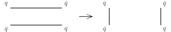
Confining potentials will be allowed to form between any two partons that have matching colour and anticolour indices. Since LC-connected partons are forced to have matching colour and anticolour indices, the “original” (LC) string topology always remains possible, but now further possibilities also exist involving partons that accidentally have matching indices, illustrated in fig. 4.
crex
{fmfgraph*}(40,20)
\fmfforce-0.15w,1.15hv1
\fmfvlabel.dist=0,label=(A)v1
\fmftopt1,tc,t2
\fmfleftl1,l2
\fmfrightr1,rc,r2
\fmfbottomb1,g12,bd,b2
\fmfvd.shape=circle,d.fill=empty,label.dist=0,d.siz=20,label=b1
\fmfvd.shape=circle,d.fill=empty,label.dist=0,d.siz=20,label=g12
\fmfvd.shape=circle,d.fill=empty,label.dist=0,d.siz=20,label=b2
\fmfvd.shape=circle,d.fill=empty,label.dist=0,d.siz=20,label=r2
\fmfvd.shape=circle,d.fill=empty,label.dist=0,d.siz=20,label=l2
\fmfplain,fore=redb1,g12
\fmfplain,fore=redg12,b2
\fmfplain,fore=redl2,r2
vs. {fmfgraph*}(40,20)
\fmfforce-0.15w,1.15hv1
\fmfvlabel.dist=0,label=(B)v1
\fmftopt1,tc,t2
\fmfleftl1,l2
\fmfrightr1,rc,r2
\fmfbottomb1,g12,bd,b2
\fmfvd.shape=circle,d.fill=empty,label.dist=0,d.siz=20,label=b1
\fmfvd.shape=circle,d.fill=empty,label.dist=0,d.siz=20,label=g12
\fmfvd.shape=circle,d.fill=empty,label.dist=0,d.siz=20,label=b2
\fmfvd.shape=circle,d.fill=empty,label.dist=0,d.siz=20,label=r2
\fmfvd.shape=circle,d.fill=empty,label.dist=0,d.siz=20,label=l2
\fmfplain,fore=redb1,g12
\fmfplain,fore=redg12,l2
\fmfplain,fore=redb2,r2
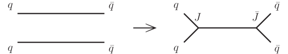
Furthermore, two colour indices are allowed to sum coherently to a single anticolour index within three separate closed index groups: [1,4,7], [2,5,8], and [3,6,9]. E.g., two quarks carrying indices 2 and 5 respectively, are allowed to appear to the rest of the event as carrying a single combined anti-8 index. These index combinations represent the antisymmetric colour combinations that were pictorially represented as Y-shaped “colour junctions” in fig. 3. A junction can therefore be interpreted as the string extension of a baryon with the baryon number () located in the centre of the Y-shape Sjostrand:2002ip . An explicit example of a parton system whose colour state includes such a possibility is shown in fig. 5.
crex2
{fmfgraph*}(40,20)
\fmfforce-0.15w,1.15hv1
\fmfvlabel.dist=0,label=(C)v1
\fmftopt1,tc,t2
\fmfleftl1,l2
\fmfrightr1,rc,r2
\fmfbottomb1,g12,bd,b2
\fmfvd.shape=circle,d.fill=empty,label.dist=0,d.siz=20,label=b1
\fmfvd.shape=circle,d.fill=empty,label.dist=0,d.siz=20,label=g12
\fmfvd.shape=circle,d.fill=empty,label.dist=0,d.siz=20,label=b2
\fmfvd.shape=circle,d.fill=empty,label.dist=0,d.siz=20,label=r2
\fmfvd.shape=circle,d.fill=empty,label.dist=0,d.siz=20,label=l2
\fmfplain,fore=redb1,g12
\fmfplain,fore=redg12,b2
\fmfplain,fore=redl2,r2
vs. {fmfgraph*}(40,20)
\fmfforce-0.15w,1.15hv1
\fmfvlabel.dist=0,label=(D)v1
\fmftopt1,tc,t2
\fmfleftl1,l2
\fmfrightr1,rc,r2
\fmfbottomb1,g12,bd,b2
\fmfvd.shape=circle,d.fill=empty,label.dist=0,d.siz=20,label=b1
\fmfvd.shape=circle,d.fill=empty,label.dist=0,d.siz=20,label=g12
\fmfvd.shape=circle,d.fill=empty,label.dist=0,d.siz=20,label=b2
\fmfvd.shape=circle,d.fill=empty,label.dist=0,d.siz=20,label=r2
\fmfvd.shape=circle,d.fill=empty,label.dist=0,d.siz=20,label=l2
\fmfplain,fore=redb1,g12
\fmfplain,fore=redg12,j1,l2
\fmfplain,fore=redb2,j2,r2
\fmfplain,fore=redj1,j2
A model for string hadronisation of such topologies was developed in Sjostrand:2002ip and has subsequently also been applied to the modelling of baryon beam remnants Sjostrand:2004pf . We reuse it here for hadronisation of junction-type colour-index combinations.
The new model can be divided into two main parts: a new treatment of the colour flow in the beam remnant and a new CR scheme. The two models are independent and can therefore in principle be combined both with each other as well as with other models. (Note, however, that the old PYTHIA 8 CR scheme is inextricably linked with the colour treatment of the beam remnant and therefore only works together with the old beam-remnant model.) Both of the models occasionally result in complicated multi-junction configurations that the existing PYTHIA hadronisation cannot handle. Rather than attempting to address these somewhat pathological topologies in detail, this problem is circumvented by a clean-up method that simplifies the structure of the resulting systems to a level that PYTHIA can handle.
The next two sections describe respectively the details of the new beam-remnant model and the new CR scheme, including technical aspects and the algorithmic implementation. Afterwards the junction clean-up method is described.
2.3.1 Colour Flow in the Beam Remnant
It being an inherently non-perturbative object, we do not expect to be able to use perturbative QCD to understand the structure of the beam remnant. Instead, we rely on conservation laws; the partons making up the beam remnant must, together with those that have been kicked out by MPI, sum up to the total energy and momentum of the beam particle, be in an overall colour-singlet state, with unit baryon number (for a proton beam), carrying the appropriate total valence content for each quark flavour, with equal numbers of sea quarks and antiquarks. The machinery used to conserve all these quantities should be consistent with whatever knowledge of QCD we possess, such as the standard single-parton-inclusive PDFs to which our framework reduces in the case of single-parton scattering.
In this work the focus is on the formation of colour-singlet states, including the use of epsilon tensors. This naturally leads to a modification of the treatment of baryon number conservation, due to the close link between baryons and the epsilon tensors in . The modelling of energy/momentum and flavour conservation is not touched relative to the existing modelling of those aspects, and thus only a small review is presented here (for more details see Sjostrand:2004pf ).
The overall algorithm can be structured as follows:
-
1.
Determine the colour structure of the already scattered partons.
-
2.
Add the minimum amount of partons needed for flavour conservation.
-
3.
Add the minimum amount of gluons required to obtain a colour-singlet state.
-
4.
Connect all colours.
-
5.
With all the partons determined find their energy fractions.
The conservation of baryon number is not listed as a separate point, but naturally follows from the formation of junctions. Let us now consider each of these points individually starting from the top.
To calculate the colour structure of the beam remnant, let us return to the DPS example of earlier. With a probability of , the two gluons form a completely incoherent state, leaving four colour charges to be compensated for in the beam remnant (two colours and two anticolours). However the three valence quarks alone are insufficient to build up a (eq. (6)), and therefore a minimum of one additional gluon is needed. Then two of the quarks can combine to form a , which can form an with the remaining valence quark, which then can enter in a with the added gluon. Conversely, if the two gluons had been in an octet state instead, the additional gluon would not have been needed. Thus, in order to determine the minimal number of gluons needed in the beam remnant, we need to know the overall colour representation of all the MPI initiators combined.
While it could be possible to choose this representation purely statistically, based on the (simplified or full) weights, we note two reasons that a lower total beam-remnant charge is likely to be preferred in nature. Firstly, to determine the most preferred configuration the string length needs to be considered. Since the beam remnants reside in the very forward regime, strings spanned between the remnant and the scattered gluons tend to be long, and as such a good approximation is to minimise the number of strings spanned to the beam. This corresponds to preferring a low-charge colour-multiplet state for the remnant, and as a consequence also minimises the number of additional gluons required. Secondly, a purely stochastic selection corresponds to the assumption that the scattered partons are uncorrelated in colour space. For hard MPIs (at ), this is presumably a good approximation, since the typical space-time separation of the collisions are such that two independent interactions do not have time to communicate. This is illustrated by fig. 6(a). However, after the initial-state radiation is added, the lower evolution scale implies larger spatial wavefunctions, allowing for interference between different interactions, illustrated by fig. 6(b). An additional argument is that at a low evolution scale the number of partons is low, thus to combine to an overall singlet the correlation between the few individual partons needs to be large. To provide a complete description of this cross-talk, multi-parton densities for arbitrarily many partons would be needed, ideally including colour correlations and saturation effects. Although correlations in double-parton densities has been the topic of several recent developments Gaunt:2009re ; Flensburg:2011kj ; Blok:2011bu ; Diehl:2011yj ; Manohar:2012jr ; Manohar:2012pe ; Chang:2012nw ; Blok:2013bpa ; Snigirev:2014eua , the field is still not at a stage at which it would be straightforward to combine explicit double-parton distributions with the standard single-parton-inclusive ones (which a code like PYTHIA must be compatible with), nor to generalise them to arbitrarily many partons. The only formalism we are aware of that addresses all of these issues (in particular flavour and momentum correlations for arbitrarily many partons) while reducing to the single-parton ones for the hardest interaction remains the one developed in the context of the current PYTHIA beam-remnant model Sjostrand:2004pf . In this study, we supplement the momentum- and flavour-correlation model of Sjostrand:2004pf with a simple model of colour-space saturation effects appropriate to the -multiplet language used in this work. Noting that saturation should lead to a suppression of higher-multiplet states, we use a simple ansatz of exponential suppression with multiplet size, :
| (7) |
where is the probability to accept a multiplet of size and is a free parameter that controls the amount of suppression.
Everything stated above for the two-gluon case can be generalised to include quarks and an arbitrary number of MPI. The calculation just extends to slightly more complicated expressions:
| (8) |
where quarks enter as triplets, antiquarks as antitriplets and gluons as octets. The statistical probability to choose any specific multiplet can be calculated in a similar fashion, either in full or simplified QCD. There is however still an ambiguity in how the colours are connected. For instance consider two quarks and one antiquark forming an overall triplet state. The colour calculation will not tell us which of the quarks are in a singlet with the antiquark. In the case of ambiguities, the implementation is to choose randomly. The CR algorithm applied later may anyhow change the initial colour topology, lessening the effect of the above choice.
At the level of the technical implementation, the choice of colour state for the scattered partons is transferred to the final state particles of the event using the LC structure of the MPI and PS. For example, if the two gluons are in the octet state, one of the LHE colour tags (see Boos:2001cv ; Alwall:2006yp ) is changed accordingly, and is propagated through to the colour of the final state particles.
As a special case the overall colour structure of the beam remnant is not allowed to be a singlet. This is to avoid double-counting between diffractive and non-diffractive events. In the DPS example, if the gluons form a colour singlet, they essentially make up (part of) a pomeron, and thus should fall under the single-diffractive description. It would be interesting to look into the interplay between MPI and diffraction in more detail using the colour-multiplet language developed here, but this would require its own dedicated study, beyond the scope of this work.
The conservation of flavour is relative straightforward and follows Sjostrand:2004pf . The principle used is to add the minimum needed flavour. For example if only an s quark is scattered from a proton, the remnant will consist of an plus the three valence quarks.
With the flavour structure and colour multiplet of the beam remnant known, it is now possible to calculate explicitly how many gluons need to be added to obtain a colour-singlet state. Again the idea is to add the minimum number of gluons to the beam remnant. Colour-junction structures, which we have argued can arise naturally in the colour structure of the scattered partons, complicate this calculation slightly. To achieve an overall colour-singlet state the number of junctions minus the number of antijunctions has to match that of the beam particle. Taking this into account the minimal number of gluons is given by
| (9) |
where is the beam baryon number (1 if the beam is a baryon, 0 if the beam is a meson, and -1 if the is an antibaryon). The division by two is due to the gluons carrying two colour lines. Without junctions, the number of gluons is simply the number of colour lines to the remnant minus the number of available quarks to connect those colour lines to. It is easiest to understand how junctions change this, by noting that the creation of a junction basically takes two colour charges and turn into one anticolour. Thus the number of required connections goes down by one for each additional junction needed.
After the gluons are added, all the colour connections and junction structures are assigned randomly between the remaining colours, with one exception: if the beam particle is a baryon and a junction needs to be constructed (similarly for an antibaryon and an antijunction), two of the valence quarks will be used to form the junction structure (possibly embedded in a diquark), if they have not already been scattered in the MPIs.
With finally the full parton structure known, including both flavours and explicit colours, the last step of the construction of the beam remnant is the assignment of energy fractions ( values) to each remnant parton, according to modified PDFs. To obtain overall energy-momentum conservation, the individual partons are scaled by an overall factor. The scaling becomes slightly more complicated by the introduction of primordial . Details on the modified PDF versions and the scaling can be found in Sjostrand:2004pf .
2.3.2 Colour Flow in the Whole Event
As discussed above, the CR model is applied after the parton-shower evolution has finished (and after inclusion of the beam-remnant partons as described in the preceding subsection), just before the hadronisation. The model builds on two main principles: a simplified structure of QCD, based on indices from 1 to 9, to tell which configurations are possible; and the potential energy of the resulting string systems, as measured by the so-called measure Andersson:1998tv , to choose between the allowed configurations.
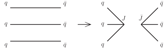
The starting point for the model is the LC configuration emerging from the showers + beam remnants. Thus between each LC-connected pair of partons a tentative dipole is constructed. This configuration is then changed by allowing two (or three) dipoles to reconnect, and this procedure is iterated until no more reconnections occur. In each step of the algorithm, four different types of reconnections can occur, illustrated in fig. 7:
-
1.
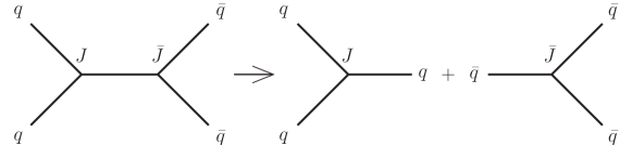
simple dipole-type reconnections involving two dipoles that exchange endpoints (fig. 7(a));
-
2.
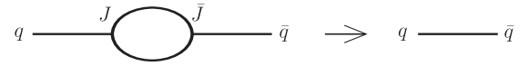
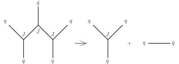
two dipoles can form a junction-antijunction structure (fig. 7(b));
-
3.
three dipoles can form a junction-antijunction structure (fig. 7(c));
-
4.
two multi-parton string systems can form a junction and an antijunction at different points along the string and connect them via their gluons (fig. 7(d)).
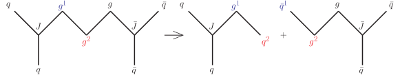
Note that, although mainly dipoles between quarks are shown in the illustrations, all dipoles (-, -, - and -) are treated in the same manner in the implementation. Within an LC dipole, the quark and antiquark are assumed to be completely colour coherent, so that the probabilities for two dipoles to be in a colour-coherent state can be found by the standard products. In full QCD, the probabilities for type I (dipole) and II (junction) reconnections for - dipoles are given by eq. (4) and (5) as and , respectively. For dipoles, the calculation is complicated slightly by the fact that eq. (1) takes into account both the colour and anticolour charges of both of the gluons. With a probability of each, either “side” (colour or anticolour) of the gluons are allowed to reconnect (for a probability that CR is allowed on both sides). And with a total probability of either one or the other side is allowed a junction-type reconnection (both sides would be equivalent to a dipole-style reconnection already counted above). For simplicity, the index rules described in the beginning of this section have been defined to treat , , and dipoles all on an equal footing. The result is a compromise of for all dipole-type reconnections and for all junction-type reconnections. Differences between and combinations still arise due to gluons being prevented from having the same colour and anticolour indices, and since the combination of two type-II reconnections is equivalent to a type-I reconnection. A comparison between the weights resulting from our simplified treatment and the multiplet weights in full QCD for the simple case of two-parton combinations was illustrated in fig. 3. Note also that the probability for a type-III reconnection among three uncorrelated dipoles (essentially creating a baryon from three uncorrelated quarks) is in full QCD (among the 27 different ways to combine 3 quarks, only one is a singlet) while it is only 2/3 as large in our model; . Although our model should be a significant step in the right direction, we therefore still expect a tendency to underestimate baryon production. When tuning the model below, we shall see that we are able to compensate for this by letting junction-type reconnections appear somewhat more energetically favourable compared with dipole-type reconnections.
To recapitulate the model implementation, each dipole is assigned a random index value between 1 and 9. Two dipoles are allowed to do a type-I reconnection if the two numbers are equal, providing the probability. Type-II reconnections are allowed if the two numbers modulo three are equal and the indices are different (e.g. 1-4 and 1-7), thereby providing the probability. Three dipoles are allowed to do the type-III reconnection if they all have the same index modulo three and are all different (1-4-7). The type-IV reconnection follows the same principles: a dipole needs to have the same index, and a junction needs to have different-but-equal-under-modulo-three index. The exact probability for type-IV reconnections depend on the number of gluons in the string.
The number of allowed colour indices can in principle be changed (the 9 above), e.g. to vary the strength of CR. However, the type-II, -III, and -IV reconnections rely on the use of modulo, thus care should be taken if junction formation is allowed. A different method to control the strength of the CR will be discussed below.
The above colour considerations only tell which new colour configurations are allowed and not whether they are preferable. To determine this, we invoke a minimisation of the string-length measure. The measure can be interpreted as the potential energy of a string, more detailed it is the area spanned by the string prior to hadronisation. It is closely connected to the total rapidity span of the string, and thereby also its total particle production. The minimisation is carried out by only allowing reconnections that lower the measure, which ensures that a local minimum is reached.
A further complication is that, while the -measure for a quark-antiquark system with any number of gluon kinks in between is neatly defined by an iterative procedure Andersson:1998tv , the measure defined there did not include junction structures. The first extension to handle these were achieved by starting from the simple measure between a quark antiquark dipole Sjostrand:2002ip :
| (10) |
where is the dipole mass squared and is a constant with dimensions of energy, of order . For high dipole masses, the “” in eq. (10) can be neglected, splitting the -measure neatly into two parts: one from the quark and one from the antiquark end (in the dipole rest frame):
| (11) |
The extension to handle a junction system used the same method, going to the junction rest-frame and adding up the “-measures” from all the three (anti-)quark ends. The end result became
| (12) |
where the energies are calculated in the junction rest frame555Note: we use a slightly different definition of here compared to the original paper Sjostrand:2002ip . This procedure worked well in the scenarios considered in that study, since all the dipoles had a relative large mass. However, in the context of our CR model, we will often be considering dipoles that have quite small masses. In that case, continuing to ignore the “” in eq. (10) can lead to arbitrarily large negative measures. Among other things, such a behaviour could allow soft particles with vanishing string lengths to have a disproportionately large impact on dipoles with a large invariant mass. Generalising this behaviour to soft junction structures results in similar effects, namely that soft particles can have a disproportionately large effect.
An alternative measure is here proposed to remove the problem with negative string lengths,
| (13) |
where the energies are calculated in the rest-frame of the dipoles. This measure is always positive definite. In the case of massless particles the -measure can be rewritten to
| (14) |
where again is the invariant mass squared of the dipole and is a constant. The two measures agree in the limit of large invariant masses (). The implementation includes a few alternative measures as options, but the above is chosen as the default measure and therefore also the one that the parameters are tuned for.
A final complication regarding the measure is that the form above cannot be used to describe the distance between two directly connected junctions. Instead the same measure as described in Sjostrand:2002ip is also used in this study (, where and are the 4-velocities of the two junction systems).
Since the -measure for junctions introduces additional approximations, a tuneable parameter is added to control the junction production. Several options for this parameter are possible and we settled on a in the -measure for junctions. A higher means a lower measure, resulting in an enhancement of the junction production. We cast the free parameter as the ratio,
| (15) |
thus a value above unity indicates an enhancement in junction production, and vice versa. The possibility of a junction enhancement can be seen as providing a crude mechanism to compensate for the intrinsic suppression of junction topologies in the colour-space model. Indeed, in the section on tuning below we find that values above unity are preferred in order to fit the observed amounts of baryon production.
In the context of CR, it is generally the dipoles with the largest invariant masses which are the most interesting; they are the ones for which reconnections can produce the largest reductions of the measure. However, as evident from the above discussion, dipoles with small invariant masses can actually be the most technically problematic to deal with. It was therefore decided to remove dipoles with an invariant mass below from the colour reconnection. Technically this is achieved by combining the small-mass pair into a new pseudo-particle. For an ordinary dipole this is a trivial task (fig. 8(a)), but if the dipole is connected to a junction the technical aspects becomes more complicated (fig. 8(b)). The easiest way to think of this is as an ordinary diquark, but in addition to these we can have digluons, which will have three ordinary (anti-)colour tags. Note that we do not intend these to represent any sort of weakly bound state; we merely use them to represent a low-invariant-mass collection of partons whose internal structure we consider uninteresting for the purpose of CR. The pseudo-particles are formed after the LC dipoles are formed, and also after any colour reconnections if the new dipoles have a mass below . Increasing will therefore lower the amount of CR. Only small effects occur for variations around the scale, however increasing beyond 1 GeV introduces a significant reduction of CR.
The complete algorithm for the colour reconnection can be summarised as below.
-
1.
Form dipoles from the LC configuration.
-
2.
Make pseudoparticles of all dipoles with mass below .
-
3.
Minimise -measure by normal string reconnections.
-
4.
Minimise -measure by junction reconnections.
-
5.
If any junction reconnections happened return to point 3.
The choice to first do the normal string reconnections before trying to form any junctions is due to the algorithm not allowing to remove any junction pairs.
Since each reconnection is required to result in a lower -measure than the previous one, the minimisation procedure is only expected to reach a local minimum. A possible extension to reach the global minimum would be to use simulated annealing 1983Sci…220..671K . This is, e.g., the approach adopted in the HERWIG++ CR model Gieseke:2012ft . However this would also require the implementation of inverse reconnections (i.e. a junction and an antijunction collapsing to form strings, and the unfolding of pseudo-particles.). Secondly the computational time needed to find the global minimum would slow down the event generation speed very significantly. For purposes of this implementation, we therefore restrict ourselves to a local deterministic minimisation here, noting that an algorithm capable of reproducing the full expected area-law exponential would be a desirable future refinement.
2.3.3 Hadronisation of Multi-Junction Systems
The existing junction hadronisation model Sjostrand:2004pf was developed mainly for the case of string systems containing a single junction (in the context of baryon-number violating SUSY decays like ). For such systems, the strategy of is to take the two legs with lowest energy in the junction rest-frame and hadronise them from their respective quark ends inwards towards the junction, until a (low) energy threshold is reached, at which point the two endpoints are combined into a diquark (which contains the junction inside). This diquark then becomes the new endpoint of the last string piece, which can then be fragmented as usual.
The case of a junction-antijunction system was also addressed in Sjostrand:2004pf (arising e.g., in the case of ), but the new treatment of the beam remnants presented here, as well as the new CR model, can produce configurations with any number of colour-connected junctions and antijunctions. This goes beyond what the existing model can handle.
The systems of equations describing such arbitrarily complicated string topologies are likely to be quite involved, with associated risks of instabilities and pathological cases. Rather than attempting to address these issues in full gory detail, we here adopt a simple “divide-and-conquer” strategy, slicing the full system into individual pieces that contain only one junction each, via the following 3 steps:
-
•
If a junction and an antijunction are connected with a single gluon between them, that gluon is forced to split into two light quarks (u,d and s) that each equally share the 4-momentum of the gluon (corresponding to ). Since the gluon is massless, the two quarks will have to be parallel (fig. 9(a)).
-
•
If a junction and an antijunction are connected with at least 2 gluons in between, the gluon pair with the highest invariant mass is found, and is split according to the string-fragmentation function. The highest invariant mass is chosen due to it having the largest phase space and being the most likely to have a string breakup occur. The split is done in such a way that the two gluons are preserved but each of them give up part of their 4-momentum to the new quark pair. The new quark that is colour-connected to one of the gluons will be parallel to the other gluon (fig. 9(b), where the indices indicate who is parallel with whom.).
-
•
After the two rules above have been applied, only directly-connected junction-antijunctions are left. If all three legs of both junctions are connected to each other, the system contains no partons and can be thrown away. If two of the legs are directly connected, the junction-antijunction system is equivalent to a single string piece and is replaced by such, see fig. 10(a). Finally, the case of a single direct junction-antijunction connection is dealt with differently, depending on whether the system contains further junction-antijunction connections or not. In the former case, illustrated in fig. 10(b), the maximum number of junctions are formed from the partons directly connected to the junction system. The remaining particles are formed into normal strings. In the example of fig. 10(b), three quarks are first removed to form a junction system; the remaining and then have no option but to form a normal string. The current method randomly selects which outgoing particles to connect with junctions. One extension would be to use the string measure to decide who combines with whom. (However the effect of this might be smaller than expected, since the majority of the multi-junction configuration comes from the beam remnant treatment, which later undergoes CR.)
For cases with a single direct junction-antijunction string piece and no further junctions in the system, illustrated in fig. 10(c), the -measure is used to determine whether the two junctions should annihilate or be kept Sjostrand:2004pf (essentially by determining whether the strings pulling on the two junctions cause them to move towards each other, towards annihilation, or away from each other). If the junctions survive, a new pair is formed by taking momentum from the other legs of the junction. Otherwise the junction topology is replaced by two ordinary strings. An option to always keep the junctions also exists.
2.3.4 Space-Time Structure
By default, we do not account for any space-time separation between different MPI systems. This is motivated by the observation that, physically, the individual MPI vertices can at most be separated by transverse distances of order the proton radius, which by definition is small compared with the length of any string long enough to fragment into multiple particles.
We do note, however, that in order for reconnections to occur between two string pieces, they should be in causal contact; if either string has already hadronised before the other forms, there is no space-time region in which reconnections between them could physically occur. In the rest frame of a hadronising string piece, we take the formation time of the corresponding QCD dipole to be given roughly by the inverse of its invariant mass, . Alternative measures (e.g., the evolution variable of the PS) could also have been used, and to allow at least a range of variations of the exact definition, a free parameter is introduced. The time at which the string piece begins to hadronise is related to the inverse of , . In order for reconnections to be possible between two string pieces, we require that they must be able to resolve each other during the time between formation and hadronisation, taking time-dilation effects caused by relative boosts into account. There are several ways in which this requirement can be formulated at the technical level, and accordingly we have implemented a few different options in the code. In principle, the two strings can be defined to be in causal contact if the relative boost parameter fulfils:
| (16) |
where is a tuneable parameter and is a fixed constant given by the typical hadronisation scale. There are however two major problems with this definition: first it is not Lorentz invariant; the two dipoles will not always agree on whether they are in causal contact or not. This can be circumvented, by either requiring both to be able to resolve each other (strict) or just either of them to be able to resolve the other (loose). Secondly, the emission of a soft gluon from an otherwise high-mass string changes significantly for each of the produced string pieces, which gives an undesirable infrared sensitivity to this measure, reminiscent of the problems associated with defining the string-length measure itself. One way to avoid this problem is to consider the first formation time of each colour line, i.e. the dipole mass at the time the corresponding colour line was first created in the shower, which we have implemented as an alternative option. No matter the exact definition of formation time and hadronisation time, all models agree that reconnection between boosted strings should be suppressed. A final extremely simple way to capture this in a Lorentz-invariant way is to apply a cut-off directly on the boost factor , which thus provides a simple alternative to the other models.
These different methods have all been implemented and are available in PYTHIA, via the mode ColourReconnection:timeDilationMode. The parameter introduced above is specified by ColourReconnection:timeDilationPar and controls the size of the allowed relative boost factor for reconnections to occur. As such it can be used to tune the amount of CR. Its optimal value will vary depending on the method used, but after the methods are tuned they produce similar results (see section 3 for details).
A final aspect related to space-time structure that deserves special mention is resonance decays. By default, these are treated separately from the rest of the event. Physically, this is well motivated for longer-lived particles (e.g., Higgs bosons), which are expected to decay and hadronise separately. For shorter-lived resonances the separation of the MPI systems and resonance decays is physically not so well motivated. E.g., most bosons and top quarks will decay before hadronisation takes place, , and as such should be allowed to interact with the particles from the MPI systems, ideally with a slightly suppressed probability due to the decay time.
Currently, only two extreme cases are implemented, corresponding to letting CR occur before or after (all) resonance decays. The corresponding flag in PYTHIA is called PartonLevel:earlyResDec. When switched on, CR is performed after all resonance decays have occurred, and all final-state partons therefore participate fully in the CR. Since no suppression with resonance lifetime is applied, this gauges the largest possible impact on resonance decays from CR. When switched off, CR is performed before resonance decays, hence involving only the beam remnant and MPI systems. It is equivalent to assuming an infinite lifetime for the resonances, and hence estimates the smallest possible impact on resonance decays from CR. An optional additional CR can be performed between the decay products of the resonance decays, with the physics motivation being studies.
To summarise, we acknowledge that the treatment of space-time separation effects and causality is still rather primitive in this model. The derivation of a more detailed formalism for these aspects would therefore be a welcome and interesting future development.
3 Constraints and Tuning
The tuning scheme follows the same procedure as for the Monash 2013 tune Skands:2014pea . However at a more limited scope, since only CR parameters, and ones strongly correlated with them, are tuned. As a natural consequence of this, the Monash tune was chosen as the baseline. As discussed in section 2.3.4, several options are available for the choice of CR time-dilation method, which naturally results in slightly different preferred parameter sets. Here, we consider the following three modes:
-
•
Mode 0: no time-dilation constraints. controls the amount of CR (mode 0);
-
•
Mode 2: time dilation using the boost factor obtained from the final-state mass of the dipoles, requiring all dipoles involved in a reconnection to be causally connected (strict);
-
•
Mode 3: time dilation as in Mode 2, but requiring only a single connection to be causally connected (loose).
This allows to investigate the consequences of some of the ambiguities in the implementation of the model. For the purpose of later studies that may want to focus on a single model, we suggest to use mode 2 as the “standard” one for the new CR. The parameters described in this section will therefore correspond to that particular model, with parameters for the others given in appendix A. Note that this section only contains the main physical parameters; for a complete list we again refer to appendix A.
3.1 Lepton Colliders
We begin with collisions. Only small effects are expected in
this environment, due to the -ordering of the shower and the absence
of MPIs. Only CR and string-fragmentation variables were studied,
since the shower was left untouched. The fragmentation model contains three main
parameters governing the kinematics of the produced hadrons: the
non-perturbative produced in string breaks, controlled by the
parameter (StringPT:sigma), and the two parameters, and , which
control the shape of the longitudinal () fragmentation
function. For pedagogical descriptions,
see e.g. Andersson:1998tv ; Skands:2012ts ; Skands:2014pea ; Sjostrand:2014zea .
Since the effects are expected to be small, we made the choice of
keeping unchanged, adjusting only the longitudinal (
and ) parameters. Changing the minimal number of parameters
also helps to disentangle the effects of CR from the retuning.
As a verification, a tune with a smaller () was
considered, however after retuning and the two tunes described the LEP
data with a similar fidelity. (The choice of testing a lower
was made since the CR model tends connect more collinear partons leading to shorter strings, but a harder
spectrum of the produced hadrons Ortiz:2013yxa .)
The determination of the two parameters of the Lund fragmentation
function, and , is complicated slightly by the fact that they
are highly correlated; choosing both of them to be quite small often
produces equally good descriptions of fragmentation spectra as
choosing both of them large, corresponding to a relatively elongated
and correlated “valley”.
By simultaneously considering both variables and comparing them to both multiplicity
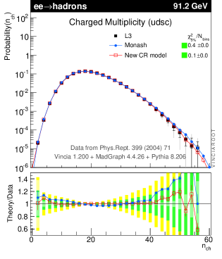
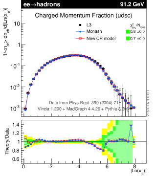
and momentum spectra, cf. fig. 11 (with the
“New CR model” curve showing
our new model, and “Monash” the baseline Monash 2013 tune), we
here settled on a
low-valued pair, as compared with the default Monash values:
StringZ:aLund = 0.38 # was 0.68
StringZ:bLund = 0.64 # was 0.98
The new CR also alters the ratio between the identified-particle yields,
especially so for baryon production due to the introduction of additional junctions.
Thus the flavour-selection parameters of the string model also need to
be retuned, by comparing with the total identified-particle yields,
see e.g. Skands:2014pea . As
expected the effects are minimal in collisions, and only
small changes are required. The modifications were therefore done with
a view to providing a better description also for colliders, but
staying within the uncertainties allowed by the LEP data. This resulted in an
adjustment of the parameters for the diquark over quark fragmentation
probability and the strangeness suppression:
StringFlav:probQQtoQ = 0.078 # was 0.081
StringFlav:probStoUD = 0.2 # was 0.217
As expected the diquark over quark probability is reduced due to the introduction of junctions. More surprisingly is the increased suppression of strange quarks, since the model a priori should not influence flavour selection. The technical implementation of the junction hadronisation does, however, introduce a slight enhancement of the strangeness production, due to an even probability for a gluon to split into an u, d or s quarks when separating junction systems. This is not visible at LEP, but at colliders the slightly lower strangeness fragmentation is favoured.
The final set of fragmentation parameters we define is more technical. For junction systems and beam remnants, a separate set of parameters controls the choice of total spin when two, already produced, quarks are combined into a diquark. Unlike diquarks produced by ordinary string breaks (whose spin is controlled by the parameter StringFlav:probQQ1toQQ0), which can only contain the light quark flavours (u, d, s), and for which the significant mass splittings between the light-flavour spin-3/2 and spin-1/2 baryon multiplets necessitates a rather strong suppression of spin-1 diquark production (relative to the naive factor 3 enhancement from spin counting), junction systems in particular can allow the formation of baryons involving heavy flavours, which have smaller mass splittings and which therefore might require less suppression of spin-1 diquarks. We note also that diquarks produced in string breakups are produced within the linear confinement of the string, whereas junction diquarks come from the combination of two already uncorrelated quarks, so there is a priori little physics reason to assume the parameters must be identical.
With the limited amount of junctions in the old model, none for and at
most two for , these parameters previously had almost no influence on measurable
observables and were therefore largely irrelevant
for tuning. With the additional junctions produced by our model, these
parameters can now give larger effects. Measurements
of higher-spin and heavy-flavour baryon states at colliders are
still rather limited though, and so far we are not aware of published directly
usable constraints from experiments.
For the time being therefore, we choose to fix
the parameters to be identical to those for the production of ordinary
diquarks in string breakups:
StringFlav:probQQ1toQQ0join = 0.027,0.027,0.027,0.027
The four components give the suppression when the heaviest quark
is u/d, s, c or b, respectively. We stress that this is merely a starting point,
hopefully to be revised soon by comparisons with new data from the LHC experiments.
3.2 Hadron Colliders
The retuning to hadron colliders consisted of tuning three main parameters:
-
•
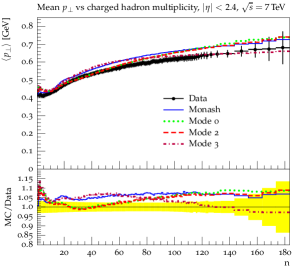
(ColourReconnection:timeDilationPar): controls the overall strength of the colour-reconnection effect via suppression of high-boost reconnections, see section 2.3.4. Can be tuned to the vs distribution.
-
•
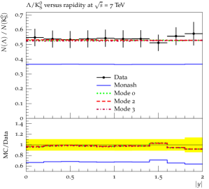
(ColourReconnection:junctionCorrection): multiplicative factor, , applied to the string-length measure for junction systems, thereby enhancing or suppressing the likelihood of junction reconnections. Controls the junction component of the baryon to meson fraction and is tuned to the ratio.
-
•
(MultiPartonInteractions:pT0Ref): lower (infrared) regularisation scale of the MPI framework. Controls the amount of low MPIs and is therefore closely related to the total multiplicity and can be tuned to the distribution.
By iteratively fitting each parameter to
its respective most sensitive curve an overall good agreement with data
was achieved
(see fig. 12) with the following parameters:
ColourReconnection:junctionCorrection = 1.2 # new parameter
ColourReconnection:timeDilationPar = 0.18 # new parameter
MultiPartonInteractions:pT0Ref = 2.15 # was 2.28
Note in particular this is the first time that PYTHIA has been able to describe the ratio in collisions while remaining consistent with LEP bounds. We explore this in more detail in section 3.4.
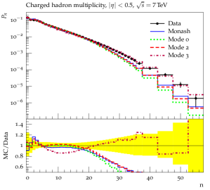
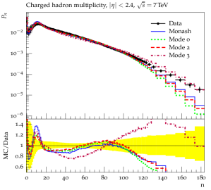
The parameter shows that a slight enhancement of junction reconnections (i.e., baryon production) is needed, relative to mesonic ones. However, given the approximations used in the implementation of especially the junction structures, such a difference is not unreasonable. Small differences between the modes can be seen in the vs and more significant differences for multiplicity distributions , cf. fig. 13. With respect to the latter, however, we note that the differences in the tails of the multiplicity distributions can be tuned away by modifying the assumed transverse matter density profile of the proton, which was kept fixed here to highlight the differences with the minimal number of retuned parameters.
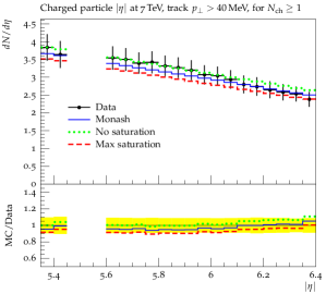
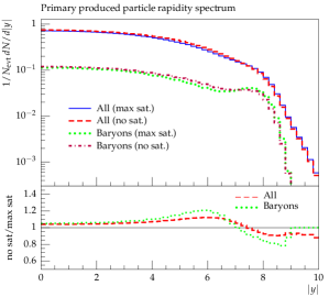
The new colour treatment of the beam remnant (BR) introduces a single new parameter
controlling the amount of saturation, cf. the discussion in
section 2.3.1. Due to the low of the BR particles,
the effects are largest in the forward direction. We therefore use the
forward charged multiplicity as measured by the TOTEM
experiment Aspell:2012ux to
compare different modelling choices of this aspect, see fig. 14(a).
The difference between no saturation666Technically:
BeamRemnants:saturation = 1E9. and
maximal saturation is about and
exhibits no shape difference over the TOTEM pseudo rapidity range.
For illustration and completeness, we may also consider what happens over the full
rapidity range, at least at the theory level. This is illustrated in
fig. 14(b). In the central region, the effect of applying
saturation is a slight decrease of the particle yield, and thus would already
have been tuned away by . It was therefore chosen to use
a relative high saturation to mimic the effect of the earlier PYTHIA beam
remnant model:
BeamRemnants:saturation = 5
We emphasise however that this is merely a starting point, and that a different balance between and may be preferred in future tuning efforts, especially ones taking a more dedicated look at the forward region. In such a study the sharing of momentum between the partons in the remnant should also be considered, since it is known to alter both particle production in the forward region and the multiplicity distributions.
An interesting signal that may help to break the relative degeneracy between and , is to look for baryons at high rapidities, which, due to the introduction of junction structures in the BR can act as further tracers of the degree to which the BR has been disturbed. This is illustrated by the lower set of curves in fig. 14(b). The effects are indeed seen to be slightly larger for baryons, however the total cross section is also significantly lower. From this simple MC study we are not able to say clearly whether such a measurement, which requires the additional non-trivial ingredient of baryon identification, would be experimentally feasible.
3.3 Direct CR Constraints?
In the preceding sections, we constrained (“retuned”) the fragmentation parameters using observables like the charged-particle multiplicity and fragmentation spectrum, which are indirectly sensitive to CR effects via the modifications caused to these spectra by the minimisation of string lengths. But what about observables with more direct sensitivity to CR effects? There are two main categories of dedicated CR studies at LEP: Fully hadronically decaying events (looking for reconnections between the two systems), and colour-flow sensitive observables in three-jet events. In this study we restrict our attention to the latter of these. A follow-up dedicated study of CR effects at colliders, both earlier as well as possible future colliders, is planned.
fmf3jeta {fmfgraph*}(85,35) \fmfleftl1,l2 \fmfrightr1,r2 \fmftopt1,t2,t3 \fmfplainv,l1 \fmfplainr1,v \fmfgluonv,t2 \fmffreeze\fmfvd.sh=circ,d.siz=5v \fmfvlabel=l1 \fmfvlabel=r1 \fmfvlabel=t2 \fmfdashes,right=0.05,fore=red,label=string,l.side=leftl1,t2 \fmfdashes,right=0.05,fore=red,label=string,l.side=leftt2,r1
fmf3jetb {fmfgraph*}(85,35) \fmfleftl1,l2 \fmfrightr1,r2 \fmftopt1,t2,t3 \fmfforce0.44w,0.98hgg1 \fmfforce0.56w,0.75hgg2 \fmfplainv,l1 \fmfplainr1,v \fmfphantomv,t2 \fmffreeze\fmfgluonv,gg1 \fmfgluonv,gg2 \fmfvd.sh=circ,d.siz=5v \fmfvlabel=l1 \fmfvlabel=r1 \fmfvlabel=gg1 \fmfvlabel=gg2 \fmfdashes,right=0.1,fore=redgg1,gg2 \fmfdashes,right=0.1,fore=redgg2,gg1 \fmfdashes,left=0.05,fore=red,label=string,l.side=rightl1,r1
Without CR, the three produced jets will in general be represented by a colour string stretched from the quark via the gluon to the antiquark, illustrated in fig. 15(a). The string pieces spanned between the quark and gluon jets lead to a relatively large particle production between these jets, while there is a suppression of particle production in the phase-space region directly between the quark and antiquark jets. However, if CR is allowed, there is a chance that two (or more) sequentially emitted gluons end up cancelling each others’ colour charges. Thus, if at least one additional gluon was produced in the FSR, the “gluon jet” may effectively become overall colour neutral, allowing it to decouple from the quark-antiquark system in colour space. This is illustrated in fig. 15(b). There is a caveat to the above, namely, if the two gluons originate from a single gluon, ie., , the two gluons must form a colour octet. In the gluon-collinear limit, this colour structure dominates and the probability for the jet to end up colour neutral should therefore be strongly suppressed, below . This aspect is not included in our model, since the history of the final state particles is not considered. The model may therefore overestimate the CR effect on three-jet events.
An additional consequence is that the jet will also have a total electric charge of zero, if all particles from the fragmentation fall within the jet. The best observable uses both of these ideas. Firstly a rapidity gap is required in order to select events with minimum radiation between the jets. This also enhances the probability that all the particles from the fragmentation falls within the jet. Secondly the jet is required to have a total charge of zero. This observable was first proposed during the LEP runs Friberg:1996xc and successively followed up by several of the experiments Abbiendi:2003ri ; Schael:2006ns ; Achard:2003ik . The studies were limited to excluding only the most extreme CR models, with no conclusions drawn between more moderate CR models and no CR; the data was located in between the two predictions.
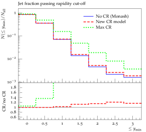
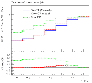
Rather than comparing our model directly on the LEP data, we took a slightly simpler approach by only considering the difference between no CR and the new CR model in the relevant observables. The difference is found to be negligible on those observables, cf. the “No CR” and “New CR” histograms in fig. 16. Thus we do not expect that the new CR model could be ruled out by these LEP constrains. We note that the small difference between with and without CR can be understood, by remembering the large focus on junction structures in the new CR model. Junction structures do not produce colour-singlet jets in the same manner as ordinary strings, and thus are not sensitive to this observable in the same way as ordinary strings reconnections. It is possible to consider a more extreme version of the new CR model where all dipoles are allowed to connect with each other, i.e. effectively replacing by unity! This is illustrated by the “max CR” histogram in fig. 16. For this unphysically extreme case the difference between the two models becomes so large it most likely would have been ruled out by the experiments. However such an extreme case would also be eliminated by just considering LHC measurements (e.g. vs ).
3.4 Suggestions for New Observables
As discussed in section 3.2, the new CR model is able to reach agreement with some key observables that have otherwise proved difficult for the string model (as implemented in PYTHIA) in the environment. In particular, subleading dipole connections that minimise the string-length measure can account for the rise in the distribution (a feature also present in earlier CR models in PYTHIA, though without the connection with subleading colour), and subleading string-junction connections can account for the observed increase in e.g. the ratio between and collisions.
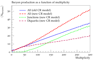
The price is (a few) new free parameters governing the CR modelling, so the question naturally arises to what extent this type of model can be distinguished clearly from other other phenomenological modelling attempts to describe the same data. All models we are aware of that simultaneously aim to describe both the LEP data and the LHC data (or and data more generally) rely on the higher colour/energy densities present in collisions to provide the extra baryons. The multiplicity scaling of the baryon production is therefore expected to be higher than the linear scaling of the diquark model. This is also what we observe, cf. fig. 17. For low multiplicity, both of the CR models agree with each other, however the increase happens faster for the new model. This shape difference in the scaling with particle multiplicity could provide an additional probe to test the new model.
One also notices that there is a significant difference between the baryon production of the old model and baryon production from diquarks in the new model. This is somewhat surprising since the hadronisation model is essentially left untouched. The explanation for this is two-fold: 1) the new CR model produces a different mass spectrum of strings (with generally lower invariant masses), and 2) low-mass strings and junction structures produce fewer additional diquarks.
The first point is illustrated in fig. 18(a), which shows the invariant-mass distribution of strings in the new and old model. In the old model, the distribution is essentially flat, and includes a significant plateau towards very large invariant masses, whereas the distribution is strongly peaked at small invariant masses in the new model. The differences arise both from the junction cleanup procedure (by which longer strings can be split by insertion of an additional quark-antiquark pair), and from the minimisation of the -measure. The old model also minimised the -measure, however this is achieved by combining strings, giving fewer but higher-mass string systems than before the CR.
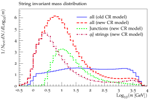
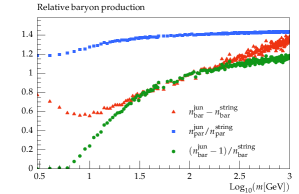
Due to energy-momentum conservation (and a greater relative importance of the quark endpoints), low-invariant-mass strings produce fewer baryons. Despite the fact that each junction system produces at least one baryon, we therefore note that this does not automatically lead to an increase in the total number of produced baryons. Since the invariant mass of a junction system is distributed on three string pieces, whereas that of a system is carried by a single string, diquarks, which are relatively heavy, can actually be quite strongly phase-space suppressed in junction topologies, especially at low invariant masses of the string system (where the majority of the junction topologies lie cf. fig. 18(a)). In addition the diquarks need to be pair produced to conserve baryon number, and the current implementation requires the pair to be on the same junction leg, leading to an even larger phase-space suppression. This effect is illustrated in fig. 18(b), where for instance a junction system with (in the peak of the mass distribution) has a five times lower probability to produce an (extra) diquark pair compared to a 10-GeV dipole string. At fixed multiplicity this effect is hidden in the tuned parameters, but can be observed by the different scaling.
Considering baryon production in more detail, the relative yield of different types of baryons is highly revealing. A collection of such yields for the different models are listed in tab. 1. For most of the baryons, the new CR model predicts about above the old model. This is in agreement with result for production shown earlier (fig. 12). There are however also some clear order-of-magnitude differences, for charm and bottom baryons. One example is production777The is a state with spin , mass and PDG code 4112 pdg2012 ., for which the new CR model predicts a rate more than a factor of 20 above that of the old model!
| Particle | New CR model () | Old CR model | ||
|---|---|---|---|---|
| string | junction | all | (all) | |
7Double heavy baryons where the last q can be any quark.
To understand how such large differences can occur, we need to recall how baryons are produced in ordinary string fragmentation. Since no charm is produced in string break-ups, the only way to produce a is to produce a -diquark and combine it with quark from the shower. However, since diquarks must have spin 1 (due to symmetry), their production is heavily suppressed relative to ones which can also exist in the far lighter spin-0 state. Enter junctions, for which there is a priori no specific penalty associated with having two legs end on same-flavour quarks as compared to different flavours. Up to some combinatorics and symmetry factors the production of and is therefore expected to be the same for junction systems, in good agreement with the observed predictions of the new CR model. As such the production of baryons like theoretically provides an excellent probe to study the relative importance between diquark- and junction-driven baryon production.
Similar results are also observed for as well as for the production of the analogous -baryons. And with the large -physics programme at the LHC, we believe this could be an interesting study, both for its physics value as well as a possible source of background for other measurements. The effect can also be seen for , however not as clearly as for charm and bottom baryons. Moreover the presence of additional suppression of strange diquarks in the string fragmentation model makes connection more complicated. We note that it can be an important validation channel however.
Due to the majority of baryons being produced by the junction mechanism in the new CR model, the baryon yields also provides a clear probe to test the spin structure of the diquarks formed from the junctions. The large difference in yield between and is due to the choice of spin suppression mentioned earlier in the tuning section. An actual measurement could be directly applied as a constraint for this variable. At least with the development of the present model, we now have a vehicle that allows to explore this type of phenomenology and interpret the findings.
We should note that the baryons considered above are excited states that rapidly decay through the emission of a pion, e.g. . As such they may be quite challenging to observe experimentally. It is therefore not a given that it will be easy to utilise measurements of these yields. But it does provide a theoretical motivation for studying the production and measurement of heavy baryons.
Another special class of baryons is the double (or triple) heavy baryons containing at least two c or b quarks. These baryons can not be formed in ordinary string fragmentation and is therefore almost non-existent in the old CR scheme. The only production mechanism is via the junctions from the beams (which also means that for collisions no double-heavy antibaryons are predicted). This is also observed in tab. 1, where only a single double-heavy baryon is produced in the 10 million events. With the large amount of junctions, the new CR model provides a natural production mechanism for double-heavy baryons, and as such the expected amount is also significantly higher than for the old CR model. The effect of massive quarks in the -measure is not well understood, however, and possible other production mechanism might also contribute, thus the estimate is most likely rather crude. Irrespectively, a measurement of double-heavy baryons probes a region of hadronisation that the current models do not describe. And it could possible also shed some light on whether the junction mechanism might be a reasonable production mechanism.
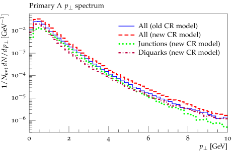
So far, we only considered total particle yields; more knowledge is available by studying more differential distributions. A natural next extension is the transverse momentum distributions. As the junctions are formed by minimising the -measure, the particles defining the junction may be expected to preferentially be moving in the same direction and thereby create a boosted baryon. This in turn leads to an expected increase in transverse momentum for such junction baryons. This is also observed in the low- region (below roughly ), where the particle production peak is higher for junction baryons (fig. 19). In the region of very high (above roughly ) the particle production is dominated by jets, for which the hard high- partons are more important than the overall boost. In addition, the perturbative gluons associated with the jet already provides a low -measure and as such limited CR is expected inside the jet regions. This leads to the high- region being occupied predominantly by baryons produced in ordinary (diquark) string-breaks.
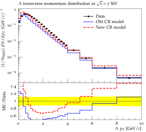
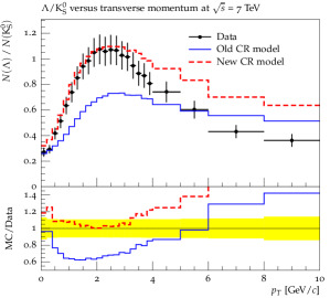
Transverse momentum spectra have already been measured for some of the more common baryon species and a comparison with the spectrum measured by CMS is given in in fig. 20. Sadly, the improvement is far less satisfactory here. The new CR model (as well as the old model) overshoots the production in the very low and the high region, whereas too few baryons are predicted in between. Thus the baryons from junctions tend to fall in the right region, however the effect is not large enough. An interesting observation is that the ratio is now well described in the low region. This shows that the problem with the distribution is not specific to baryons but is more generic. The discrepancy between data and the model for large still exists, however the baryon production in this region is primarily from diquark string breaks in jets and as such is not really unique for the new CR model. It may point to a revision needed of the spectrum of hard (leading?) baryon production in jets, which may not be unique to the environment, see Skands:2014pea .
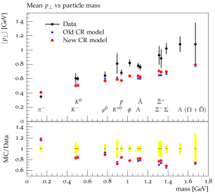
The problem in the low domain is a common theme for all heavier hadrons (i.e. anything but pions) and would be interesting to explore further. (E.g., a measurement of spectra could reveal whether it depends on the presence of strange quarks.) The PYTHIA models predict a -distribution that peaks at lower values than what is actually observed. To study this in more detail, one can calculate the average for the identified hadrons and plot it a function of their mass, as done e.g. by the STAR collaboration for collisions at Abelev:2006cs . In purely longitudinal string fragmentation the expected result is a roughly flat curve, since no correlation between the mass of the particle and is present. The flat prediction is altered when hadron decays and jet physics are included, leading to the curve seen in fig. 21. The prediction is also altered if the string is boosted (e.g., by partonic string endpoints), the boost is transferred to the final particles and for the same boost velocity a heavy particle will gain more than a light one. This effect can be enhanced by CR, since minimisation of the -measure prefers reconnections among partons moving in the same direction, thus creating boosted strings Ortiz:2013yxa . CR is therefore expected to give a sharper rise of the vs mass distribution. Unfortunately, we do not observe this expected effect at any significant level (fig. 21). To be candid, it is disappointing that the new model does not appear to address this problem at all. At the very least, it leaves room open for criticism and possibly additional new physics. Of special interest in this context are possible collective phenomena, such as (gas-like) hadron reinteractions or (hydro-like) flow, either of which could provide a (weak or strong, respectively) velocity-equalising component, and at least the latter has been applied successfully in the context of the EPOS model Pierog:2013ria . So-called “colour ropes” (strings carrying more than one unit of charge and hence having a higher tension) can also generate harder momentum spectra, while remaining within a string context, as was recently explored in Bierlich:2014xba . These effects are generally not expected to be present at the relatively low energy density in collisions at a centre-of-mass energy of 200 GeV, however. It would therefore be of great interest to redo the measurement in detail at LHC energies, for high- and low-multiplicity samples and/or in the underlying event, to study whether the slope is steeper at the higher energy densities.
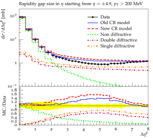
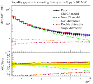
Finally, we emphasise that the rapidity gap survival is heavily affected by the choice of CR model Edin:1995gi ; Rathsman:1998tp . The explanation is similar to that of the three-jet LEP measurement, where the reconnected colour-singlet jet produces a rapidity gap to the other jets. The old CR model combines different strings into a single larger string, and thereby covers the same rapidity span, essentially adding kinks to an already existing string topology. Instead the new model can produce the colour-singlet union of particles in the same rapidity region. The new model is therefore expected to produce more rapidity gaps compared with the old model, which is also what we observe in fig. 22. The new model predictions are significantly above the data in the mid-range rapidity region for low cut-offs. (For higher cuts the effect vanishes, due to the partonic description being more influential on the rapidity gap survival.) We therefore emphasise that the new CR scenario should in principle be accompanied by a retuning of diffractive parameters. This is not straightforward however, and involves not only the shown rapidity-gap survival distributions, but several other measurements at different energies. It was therefore deemed beyond the scope of this study to perform a retuning of the diffractive components and we limit ourselves to pointing out the interplay. A future dedicated study of this aspect could also well incorporate a study of the interference between the new BR model and diffractive events.
4 Application to Top Mass Measurements at Hadron Colliders
Colour reconnections contribute one of the dominant uncertainties on current experimental top-mass extractions in hadronic channels (see e.g. the mini-review in Juste:2013dsa ), and their size was recently reexamined in the context of several simplified CR schemes Argyropoulos:2014zoa . It is thus interesting to consider our new CR model in the same framework. We follow ref. Argyropoulos:2014zoa , to which we refer for details on selection of the events and top mass reconstruction procedure.
Briefly stated, the idea is to select semi-leptonic top events, using the charged lepton and escaping neutrino mainly for tagging and then reconstruct the top mass from the hadronic decay. A mass window around the W mass is required and the raw top mass is extracted by fitting the invariant mass distribution of the three jets with a skewed Gaussian distribution, which fits the distributions better than a standard Gaussian Argyropoulos:2014zoa . For the models/tunes considered in this work (details below), the resulting shift on the calibrated top mass is below 200 MeV, which is comparable with the current level of CR uncertainty on the measurements Aaltonen:2012va ; Chatrchyan:2012cz ; Abazov:2014dpa ; Aad:2015nba and far below some of the “devil’s-advocate” toy models considered in Argyropoulos:2014zoa . Characteristic for those models is that they allow some fraction of reconnections where the measure is increased, whereas all the models considered here involve a minimisation of , one way or another.
We compare six models: no CR, the existing (default) PYTHIA 8 CR model with and without early resonance decays (ERD), the new baseline CR model with and without ERD, and the new CR with maximal CR and ERD. Since the largest effect is expected for ERD, the maximal CR scenario is only considered with ERD switched on. Two versions of the “no CR” scenario were considered, one in which CR was simply switched off without any further changes (resulting in significant increase in central hadron multiplicity) and the other a semi-tuned version, where the activity () in the central region () for ND events was retuned. A similar approach is used for the maximal CR models, where again a non-tuned version and retuned version are considered. It should be noted that neither of the retuned models provide a good description of all MB data (for instance is described by neither tune). Since none of the models considered exhibit any top-specific behaviour, no additional retuning to top events was needed. The results are collected in tab. 2.
| Model | [GeV] | [GeV] | [GeV] |
|---|---|---|---|
| no CR | 0 | 0 | |
| default ERD | |||
| default | |||
| new model ERD | |||
| new model | |||
| max CR ERD | |||
| no CR (tuned) | |||
| max CR (tuned) |
The first observation is the large difference between the no CR model and the non ERD models for ( MeV). Since no CR is performed for the top decay products, not much of difference was expected, and any difference observed has to reside entirely in the underlying event (UE). The CR models considered lower the total string length, and thereby the activity in the UE, which directly influences the non-scaled top mass. Since the “no CR” model uses the same tune parameters as the CR models, it has a too high activity in the UE, leading to the negative mass shifts seen. After retuning to a similar activity in the central region, the “no CR (tuned)” model agrees with the default CR scenario within the statistical uncertainty. This emphasises the importance of using consistent UE tunes for this type of exercise, though we also note that after recalibration by the hadronic mass, the rescaled top mass is remarkably stable.
For the ERD models the above shift in UE is still present, but the UE is now also allowed to reconnect with the top decay products. Therefore, an UE parton in close proximity to a jet from the top decay will have a large probability to be reconnected with the jet. This will result in narrower jets, leading to less of the energy falling outside the jet cone, and thereby a larger top mass. This is in agreement with the simulations, where the ERD results are above the non-ERD results. But the effect is smaller than that of the UE activity, thus the overall shift is still negative compared to the non-tuned no CR model.
Both of the above effects are magnified in the maximal CR scenario. We remind the reader that in this scenario, the suppression of subleading connections is switched off, hence this should be considered an unphysical extreme variation. Coincidentally, however, the two effects end up approximately canceling. A similar retuning of the central activity as above, “max CR (tuned)”, shows a significant increase in the top mass shift of more than one GeV with respect to the tuned no CR model, though again, the mass calibration removes most of it.
The fact that the rescaled top mass () is less sensitive to CR is due to a cancellation between CR in the W mass and the top mass. This is in perfect agreement with the simulations, where the deviation for all rescaled masses are below their respective non-rescaled deviations. On the other hand, this means that any interpretation of where the variations between the models arise becomes extremely difficult. We will therefore refrain from attempting this, and instead purely discuss the numerical values in term of the uncertainty on the top mass.
For the rescaled top mass, the differences between the models stay below 200 MeV. This is slightly less than what was observed earlier even for identical CR models (default) Argyropoulos:2014zoa . The variations in the results can be attributed to a new tune combined with a change in the PS for events. We regard the smaller differences as somewhat coincidental however, and further work is needed to genuinely improve our understanding of CR effects in the top mass measurement. What we can say at least is that the results from the new model lie within those from the default CR model, and therefore do not generate a need for larger uncertainties. Even the maximal CR, which is our attempt to mimic the very large shifts seen for models that ignore MB/UE constraints, does not change this picture. Instead a pattern emerges, namely that whenever the minimisation of the measure is used as a guideline for the CR, the shifts stay below 300 MeV (taking the models studied in Argyropoulos:2014zoa into account as well). The reason for this is two-fold: firstly the coherence of the PS ensures that the jet structure is not too significantly altered; secondly, the alterations are realised in a systematic fashion leading to a similar shift in both the top and the W mass, implying that the hadronic mass recalibration is highly robust. An increased understanding of this interplay could potentially lower the uncertainty even further.
Since these models are mainly constrained by measurements, further gains can also be achieved by improving and extending the programme of measurements sensitive to CR effects. A few new observables targeting top events specifically were already suggested in Argyropoulos:2014zoa . In the context of top mass uncertainties, such observables are of course especially relevant, as this is the closest to in-situ constraints as can be obtained, mimising the “extrapolation” that the model has to cover between the constraint and measurement environments.
In order to establish whether the small effects on predicted by -minimising models are indeed conservative or not, it would be of crucial importance to test these models as directly as possible in a variety of environments, top included. The fact that our new CR models do not yet give good descriptions of identified-particle spectra should, in this context, be seen as a warning that there can be additional non-perturbative uncertainties left unaccounted for, possibly of a dynamical origin.
5 Summary and Outlook
The question “between which partons do confining potentials arise?” is a fundamental one in non-perturbative QCD, which any attempt at modelling the process of hadronisation must address. In the leading-colour approximation and neglecting beam-remnant correlations, this is relatively simple: there is a one-to-one mapping between perturbative QCD dipoles and string pieces / clusters. In this paper, we have attempted to take a first step beyond leading colour, by including a randomisation over the set of possible subleading-colour topologies, with probabilities chosen according to a simplified version of the colour algebra.
We present the argument that while the LC approximation may be quite good in the environment of collisions (more specifically in the absence of multi-parton interactions), we expect very significant deviations from it in collisions, where the survival of the strict LC topology should be heavily suppressed. Although the probability for a subleading colour connection to be possible between any given pair of (uncorrelated) partons is only roughly , it becomes increasingly unlikely not to have any such connections as the number of uncorrelated partons increases, as e.g. in the case when considering MPI.
This implies that a complex multi-parton system will in general have several different string/cluster configurations open to it, at the time of hadronisation; the LC one is only one among many possibilities. We invoke the string-length measure to choose which one is preferred, so far via a simple winner-takes-all algorithm that does not purport to always find the global minimum. Nonetheless, we believe that this model represents a significant step in the right direction, allowing us to probe for the first time the effects of subleading colour on hadronisation in a way that may be said to be systematic and consistent with (a simplified version of) QCD.
One noteworthy new aspect of our work is the use of string junctions to represent antisymmetric colour combinations, such as two colours combining to form an overall anticolour. This provides a new source of baryon production, with properties qualitatively different from the standard diquark scenario. We have shown that this aspect allows to reconcile measured baryon/meson ratios with the string model in both and collisions simultaneously. However, we caution that the shapes of the spectra are still not well described. We had anticipated that the preference of reconnections to produce boosted string pieces should lead to an enhancement of the especially for heavier hadrons, but the magnitude of this effect observed in our model is still far too low to explain the data.
We emphasised that there is a conceptual difference between colour connections and colour reconnections. The former is related to colour-space ambiguities, such as the unknown colour correlations between different MPI initiators or the subleading-colour connections explored in this work. Colour reconnections are related to dynamical reconfigurations of the colour/string space, via perturbative gluon exchanges or non-perturbative string interactions; i.e., they involve momentum exchange as well. We did not explore effects of the latter type directly in this work, though we note that the fairly realistic string-interaction scenarios constructed by Khoze and Sjöstrand in the context of studies Sjostrand:1993hi ; Khoze:1994fu ; Khoze:1999up also feature string-length minimisation; hence it is possible that our tuned parameters effectively attempt to cover both types. If so, the fact that the momentum spectra remain discrepant may point to the need for dynamical CR.
Finally, we presented a few suggestions for additional observables, the measurement of which would give further insight and possibly help to distinguish both physical and unphysical CR models, as well as other ideas such as models based on colour ropes Andersson:1991er ; Bierlich:2014xba , hydrodynamics Pierog:2013ria , or (non-hydro) hadron rescattering. We ended by considering the simplified top-mass analysis of Argyropoulos:2014zoa and conclude that the models presented here lead to shifts in the top mass of order 200 MeV, which is within the current level of non-perturbative uncertainties on the measurements.
Acknowledgements
Many thanks to T. Sjöstrand for his valuable comments on both our physics and our code. JRC thanks the CERN theory unit for hospitality during the main part of this study. Work supported in part by the Swedish Research Council, contract number 621-2013-4287, in part by the MCnetITN FP7 Marie Curie Initial Training Network, contract PITN- GA-2012-315877, and in part by the Australian Research Council, contract FT130100744.
Appendix A Model parameters
A complete list of all the parameters that differ from the Monash tune for the three different models are listed in the table below.
| Parameter | Monash | Mode 0 | Mode 2 | Mode 3 |
| StringPT:sigma | = 0.335 | = 0.335 | = 0.335 | = 0.335 |
| StringZ:aLund | = 0.68 | = 0.36 | = 0.36 | = 0.36 |
| StringZ:bLund | = 0.98 | = 0.56 | = 0.56 | = 0.56 |
| StringFlav:probQQtoQ | = 0.081 | = 0.078 | = 0.078 | = 0.078 |
| StringFlav:ProbStoUD | = 0.217 | = 0.2 | = 0.2 | = 0.2 |
| StringFlav:probQQ1toQQ0join | = 0.5, | = 0.0275, | = 0.0275, | = 0.0275, |
| 0.7, | 0.0275, | 0.0275, | 0.0275, | |
| 0.9, | 0.0275, | 0.0275, | 0.0275, | |
| 1.0 | 0.0275 | 0.0275 | 0.0275 | |
| MultiPartonInteractions:pT0Ref | = 2.28 | = 2.12 | = 2.15 | = 2.05 |
| BeamRemnants:remnantMode | = 0 | = 1 | = 1 | = 1 |
| BeamRemnants:saturation | - | = 5 | = 5 | = 5 |
| ColourReconnection:mode | = 0 | = 1 | = 1 | = 1 |
| ColourReconnection:allowDoubleJunRem | = on | = off | = off | = off |
| ColourReconnection:m0 | - | = 2.9 | = 0.3 | = 0.3 |
| ColourReconnection:allowJunctions | - | = on | = on | = on |
| ColourReconnection:junctionCorrection | - | = 1.43 | = 1.20 | = 1.15 |
| ColourReconnection:timeDilationMode | - | = 0 | = 2 | = 3 |
| ColourReconnection:timeDilationPar | - | - | = 0.18 | = 0.073 |
References
- (1) G. Dissertori, I. Knowles, and M. Schmelling, Quantum Chromodynamics — High energy experiments and theory. Oxford Science Publications, 2003.
- (2) P. Skands, “Introduction to QCD,” arXiv:1207.2389 [hep-ph]. Lectures given at TASI 2012.
- (3) A. Buckley, J. Butterworth, S. Gieseke, D. Grellscheid, S. Höche, et al., “General-purpose event generators for LHC physics,” Phys.Rept. 504 (2011) 145–233, arXiv:1101.2599 [hep-ph].
- (4) R. D. Ball, S. Carrazza, L. Del Debbio, S. Forte, J. Gao, et al., “Parton Distribution Benchmarking with LHC Data,” JHEP 1304 (2013) 125, arXiv:1211.5142 [hep-ph].
- (5) E. Boos, M. Dobbs, W. Giele, I. Hinchliffe, J. Huston, et al., “Generic user process interface for event generators,” arXiv:hep-ph/0109068 [hep-ph].
- (6) J. Alwall, A. Ballestrero, P. Bartalini, S. Belov, E. Boos, et al., “A Standard format for Les Houches event files,” Comput.Phys.Commun. 176 (2007) 300–304, arXiv:hep-ph/0609017 [hep-ph].
- (7) A. van Hameren, C. Papadopoulos, and R. Pittau, “Automated one-loop calculations: A Proof of concept,” JHEP 0909 (2009) 106, arXiv:0903.4665 [hep-ph].
- (8) F. Cascioli, P. Maierhofer, and S. Pozzorini, “Scattering Amplitudes with Open Loops,” Phys.Rev.Lett. 108 (2012) 111601, arXiv:1111.5206 [hep-ph].
- (9) J. Alwall, M. Herquet, F. Maltoni, O. Mattelaer, and T. Stelzer, “MadGraph 5 : Going Beyond,” JHEP 1106 (2011) 128, arXiv:1106.0522 [hep-ph].
- (10) S. Alioli, S. Badger, J. Bellm, B. Biedermann, F. Boudjema, et al., “Update of the Binoth Les Houches Accord for a standard interface between Monte Carlo tools and one-loop programs,” Comput.Phys.Commun. 185 (2014) 560–571, arXiv:1308.3462 [hep-ph].
- (11) G. Cullen, H. van Deurzen, N. Greiner, G. Heinrich, G. Luisoni, et al., “GS-2.0: a tool for automated one-loop calculations within the Standard Model and beyond,” Eur.Phys.J. C74 no. 8, (2014) 3001, arXiv:1404.7096 [hep-ph].
- (12) J. Alwall, R. Frederix, S. Frixione, V. Hirschi, F. Maltoni, et al., “The automated computation of tree-level and next-to-leading order differential cross sections, and their matching to parton shower simulations,” JHEP 1407 (2014) 079, arXiv:1405.0301 [hep-ph].
- (13) G. Gustafson and U. Pettersson, “Dipole Formulation of QCD Cascades,” Nucl.Phys. B306 (1988) 746.
- (14) T. Sjöstrand and P. Z. Skands, “Transverse-momentum-ordered showers and interleaved multiple interactions,” Eur.Phys.J. C39 (2005) 129–154, arXiv:hep-ph/0408302 [hep-ph].
- (15) Z. Nagy and D. E. Soper, “Matching parton showers to NLO computations,” JHEP 0510 (2005) 024, arXiv:hep-ph/0503053 [hep-ph].
- (16) W. T. Giele, D. A. Kosower, and P. Z. Skands, “A simple shower and matching algorithm,” Phys.Rev. D78 (2008) 014026, arXiv:0707.3652 [hep-ph].
- (17) M. Dinsdale, M. Ternick, and S. Weinzierl, “Parton showers from the dipole formalism,” Phys.Rev. D76 (2007) 094003, arXiv:0709.1026 [hep-ph].
- (18) S. Schumann and F. Krauss, “A Parton shower algorithm based on Catani-Seymour dipole factorisation,” JHEP 0803 (2008) 038, arXiv:0709.1027 [hep-ph].
- (19) S. Plätzer and S. Gieseke, “Coherent Parton Showers with Local Recoils,” JHEP 1101 (2011) 024, arXiv:0909.5593 [hep-ph].
- (20) K. Hamilton, P. Nason, and G. Zanderighi, “MINLO: Multi-Scale Improved NLO,” JHEP 1210 (2012) 155, arXiv:1206.3572 [hep-ph].
- (21) L. Lönnblad and S. Prestel, “Merging Multi-leg NLO Matrix Elements with Parton Showers,” JHEP 1303 (2013) 166, arXiv:1211.7278 [hep-ph].
- (22) L. Hartgring, E. Laenen, and P. Skands, “Antenna Showers with One-Loop Matrix Elements,” JHEP 1310 (2013) 127, arXiv:1303.4974 [hep-ph].
- (23) B. Andersson, The Lund model. Camb. Monogr. Part. Phys. Nucl. Phys. Cosmol., 1997.
- (24) B. Andersson, G. Gustafson, G. Ingelman, and T. Sjostrand, “Parton Fragmentation and String Dynamics,” Phys.Rept. 97 (1983) 31–145.
- (25) G. Bali and K. Schilling, “Static quark - anti-quark potential: Scaling behavior and finite size effects in SU(3) lattice gauge theory,” Phys.Rev. D46 (1992) 2636–2646.
- (26) Particle Data Group Collaboration, J. Beringer et al., “Review of particle physics,” Phys. Rev. D86 (2012) 010001.
- (27) G. Gustafson, “Dual Description of a Confined Color Field,” Phys.Lett. B175 (1986) 453.
- (28) T. Sjöstrand, S. Mrenna, and P. Skands, “PYTHIA 6.4 physics and manual,” JHEP 05 (2006) 026, hep-ph/0603175.
- (29) T. Sjöstrand, S. Mrenna, and P. Skands, “A brief introduction to PYTHIA 8.1,” Comput. Phys. Commun. 178 (2008) 852–867, arXiv:0710.3820 [hep-ph].
- (30) T. Sjöstrand, S. Ask, J. R. Christiansen, R. Corke, N. Desai, et al., “An Introduction to PYTHIA 8.2,” Comput.Phys.Commun. 191 (2015) 159–177, arXiv:1410.3012 [hep-ph].
- (31) A. Buckley, H. Hoeth, H. Lacker, H. Schulz, and J. E. von Seggern, “Systematic event generator tuning for the LHC,” Eur.Phys.J. C65 (2010) 331–357, arXiv:0907.2973 [hep-ph].
- (32) N. Firdous and G. Rudolph, “Tuning of PYTHIA6 to Minimum Bias Data,” EPJ Web Conf. 60 (2013) 20056.
- (33) N. Fischer, S. Gieseke, S. Plätzer, and P. Skands, “Revisiting radiation patterns in collisions,” Eur.Phys.J. C74 no. 4, (2014) 2831, arXiv:1402.3186 [hep-ph].
- (34) P. Skands, S. Carrazza, and J. Rojo, “Tuning PYTHIA 8.1: the Monash 2013 Tune,” Eur.Phys.J. C74 no. 8, (2014) 3024, arXiv:1404.5630 [hep-ph].
- (35) OPAL Collaboration, G. Abbiendi et al., “Tests of models of color reconnection and a search for glueballs using gluon jets with a rapidity gap,” Eur.Phys.J. C35 (2004) 293–312, arXiv:hep-ex/0306021 [hep-ex].
- (36) L3 Collaboration, P. Achard et al., “Search for color reconnection effects in hadrons through particle flow studies at LEP,” Phys.Lett. B561 (2003) 202–212, arXiv:hep-ex/0303042 [hep-ex].
- (37) L3 Collaboration, P. Achard et al., “Search for color singlet and color reconnection effects in hadronic decays at LEP,” Phys.Lett. B581 (2004) 19–30, arXiv:hep-ex/0312026 [hep-ex].
- (38) DELPHI Collaboration, M. Siebel, “A Study of the charge of leading hadrons in gluon and quark fragmentation,” arXiv:hep-ex/0505080 [hep-ex].
- (39) OPAL Collaboration, G. Abbiendi et al., “Colour reconnection in at s**(1/2) = 189-GeV - 209-GeV,” Eur.Phys.J. C45 (2006) 291–305, arXiv:hep-ex/0508062 [hep-ex].
- (40) ALEPH Collaboration, S. Schael et al., “Test of Colour Reconnection Models using Three-Jet Events in Hadronic Z Decays,” Eur.Phys.J. C48 (2006) 685–698, arXiv:hep-ex/0604042 [hep-ex].
- (41) DELPHI Collaboration, J. Abdallah et al., “Investigation of colour reconnection in WW events with the DELPHI detector at LEP-2,” Eur.Phys.J. C51 (2007) 249–269, arXiv:0704.0597 [hep-ex].
- (42) ALEPH Collaboration, S. Schael et al., “Measurement of the boson mass and width in collisions at LEP,” Eur.Phys.J. C47 (2006) 309–335, arXiv:hep-ex/0605011 [hep-ex].
- (43) T. Sjöstrand and V. A. Khoze, “On Color rearrangement in hadronic W+ W- events,” Z.Phys. C62 (1994) 281–310, arXiv:hep-ph/9310242 [hep-ph].
- (44) ALEPH, DELPHI, L3, OPAL, LEP Electroweak Collaboration, S. Schael et al., “Electroweak Measurements in Electron-Positron Collisions at W-Boson-Pair Energies at LEP,” Phys.Rept. 532 (2013) 119–244, arXiv:1302.3415 [hep-ex].
- (45) G. Marchesini and B. Webber, “Simulation of QCD Jets Including Soft Gluon Interference,” Nucl.Phys. B238 (1984) 1.
- (46) T. Sjöstrand and M. van Zijl, “A Multiple Interaction Model for the Event Structure in Hadron Collisions,” Phys.Rev. D36 (1987) 2019.
- (47) S. Gieseke, C. Rohr, and A. Siodmok, “Colour reconnections in Herwig++,” Eur.Phys.J. C72 (2012) 2225, arXiv:1206.0041 [hep-ph].
- (48) Ames-Bologna-CERN-Dortmund-Heidelberg-Warsaw Collaboration, A. Breakstone et al., “Multiplicity Dependence of Transverse Momentum Spectra at ISR Energies,” Phys.Lett. B132 (1983) 463.
- (49) UA1 Collaboration, C. Albajar et al., “A Study of the General Characteristics of Collisions at = 0.2-TeV to 0.9-TeV,” Nucl.Phys. B335 (1990) 261.
- (50) CDF Collaboration, D. Acosta et al., “Soft and hard interactions in collisions at 1800-GeV and 630-GeV,” Phys.Rev. D65 (2002) 072005.
- (51) CDF Collaboration, T. Aaltonen et al., “Measurement of Particle Production and Inclusive Differential Cross Sections in p anti-p Collisions at s**(1/2) = 1.96-TeV,” Phys.Rev. D79 (2009) 112005, arXiv:0904.1098 [hep-ex].
- (52) CMS Collaboration, V. Khachatryan et al., “Charged particle multiplicities in interactions at , 2.36, and 7 TeV,” JHEP 1101 (2011) 079, arXiv:1011.5531 [hep-ex].
- (53) ATLAS Collaboration, G. Aad et al., “Charged-particle multiplicities in pp interactions measured with the ATLAS detector at the LHC,” New J.Phys. 13 (2011) 053033, arXiv:1012.5104 [hep-ex].
- (54) ALICE Collaboration, B. B. Abelev et al., “Multiplicity dependence of the average transverse momentum in pp, p-Pb, and Pb-Pb collisions at the LHC,” Phys.Lett. B727 (2013) 371–380, arXiv:1307.1094 [nucl-ex].
- (55) A. Karneyeu, L. Mijovic, S. Prestel, and P. Skands, “MCPLOTS: a particle physics resource based on volunteer computing,” Eur.Phys.J. C74 (2014) 2714, arXiv:1306.3436 [hep-ph].
- (56) R. Corke and T. Sjöstrand, “Interleaved Parton Showers and Tuning Prospects,” JHEP 1103 (2011) 032, arXiv:1011.1759 [hep-ph].
- (57) P. Z. Skands and D. Wicke, “Non-perturbative QCD effects and the top mass at the Tevatron,” Eur.Phys.J. C52 (2007) 133–140, arXiv:hep-ph/0703081 [HEP-PH].
- (58) CDF Collaboration, T. Aaltonen et al., “Precision Top-Quark Mass Measurements at CDF,” Phys.Rev.Lett. 109 (2012) 152003, arXiv:1207.6758 [hep-ex].
- (59) CMS Collaboration, S. Chatrchyan et al., “Measurement of the top-quark mass in events with lepton+jets final states in collisions at TeV,” JHEP 1212 (2012) 105, arXiv:1209.2319 [hep-ex].
- (60) CDF, D0 Collaboration, T. A. Aaltonen et al., “Combination of measurements of the top-quark pair production cross section from the Tevatron Collider,” Phys.Rev. D89 (2014) 072001, arXiv:1309.7570 [hep-ex].
- (61) CMS Collaboration, S. Chatrchyan et al., “Measurement of the top-quark mass in all-jets events in pp collisions at =7 TeV,” Eur.Phys.J. C74 (2014) 2758, arXiv:1307.4617 [hep-ex].
- (62) ATLAS, CDF, CMS, D0 Collaboration, “First combination of Tevatron and LHC measurements of the top-quark mass,” arXiv:1403.4427 [hep-ex].
- (63) D0 Collaboration, V. M. Abazov et al., “Precision measurement of the top-quark mass in lepton+jets final states,” Phys.Rev.Lett. 113 (2014) 032002, arXiv:1405.1756 [hep-ex].
- (64) ATLAS Collaboration, G. Aad et al., “Measurement of the top quark mass in the and channels using TeV ATLAS data,” arXiv:1503.05427 [hep-ex].
- (65) A. Juste, S. Mantry, A. Mitov, A. Penin, P. Skands, et al., “Determination of the top quark mass circa 2013: methods, subtleties, perspectives,” Eur.Phys.J. C74 no. 10, (2014) 3119, arXiv:1310.0799 [hep-ph].
- (66) V. A. Khoze and T. Sjöstrand, “Color correlations and multiplicities in top events,” Phys.Lett. B328 (1994) 466–476, arXiv:hep-ph/9403394 [hep-ph].
- (67) V. A. Khoze and T. Sjöstrand, “QCD interconnection studies at linear colliders,” Eur.Phys.J.direct C2 (2000) 1, arXiv:hep-ph/9912297 [hep-ph].
- (68) J. Rathsman, “A Generalized area law for hadronic string re-interactions,” Phys.Lett. B452 (1999) 364–371, arXiv:hep-ph/9812423 [hep-ph].
- (69) M. Sandhoff and P. Z. Skands, “Colour annealing - a toy model of colour reconnections,” arXiv:hep-ph/0604120 [hep-ph]. FERMILAB-CONF-05-518-T.
- (70) C. Buttar, S. Dittmaier, V. Drollinger, S. Frixione, A. Nikitenko, et al., “Les houches physics at TeV colliders 2005, standard model and Higgs working group: Summary report,” arXiv:hep-ph/0604120 [hep-ph].
- (71) S. Argyropoulos and T. Sjöstrand, “Effects of color reconnection on final states at the LHC,” JHEP 1411 (2014) 043, arXiv:1407.6653 [hep-ph].
- (72) T. Pierog, I. Karpenko, J. Katzy, E. Yatsenko, and K. Werner, “EPOS LHC : test of collective hadronization with LHC data,” arXiv:1306.0121 [hep-ph].
- (73) CMS Collaboration, V. Khachatryan et al., “Observation of Long-Range Near-Side Angular Correlations in Proton-Proton Collisions at the LHC,” JHEP 1009 (2010) 091, arXiv:1009.4122 [hep-ex].
- (74) K. Werner, I. Karpenko, and T. Pierog, “The ’Ridge’ in Proton-Proton Scattering at 7 TeV,” Phys.Rev.Lett. 106 (2011) 122004, arXiv:1011.0375 [hep-ph].
- (75) A. Ortiz Velasquez, P. Christiansen, E. Cuautle Flores, I. Maldonado Cervantes, and G. Paic, “Color Reconnection and Flowlike Patterns in Collisions,” Phys.Rev.Lett. 111 no. 4, (2013) 042001, arXiv:1303.6326 [hep-ph].
- (76) B. Andersson and P. Henning, “On the dynamics of a color rope: The Fragmentation of interacting strings and the longitudinal distributions,” Nucl.Phys. B355 (1991) 82–105.
- (77) C. Bierlich, G. Gustafson, L. Lönnblad, and A. Tarasov, “Effects of Overlapping Strings in pp Collisions,” JHEP 1503 (2015) 148, arXiv:1412.6259 [hep-ph].
- (78) R. Corke and T. Sjöstrand, “Multiparton Interactions and Rescattering,” JHEP 1001 (2010) 035, arXiv:0911.1909 [hep-ph].
- (79) H. Fritzsch, “Producing Heavy Quark Flavors in Hadronic Collisions: A Test of Quantum Chromodynamics,” Phys.Lett. B67 (1977) 217.
- (80) A. Ali, J. Körner, G. Kramer, and J. Willrodt, “Nonleptonic Weak Decays of Bottom Mesons,” Z.Phys. C1 (1979) 269.
- (81) H. Fritzsch, “How to Discover the Mesons,” Phys.Lett. B86 (1979) 343.
- (82) D. Eriksson, G. Ingelman, and J. Rathsman, “Colour rearrangements in B-meson decays,” Phys.Rev. D79 (2009) 014011, arXiv:0811.2651 [hep-ph].
- (83) W. Buchmüller and A. Hebecker, “A Parton model for diffractive processes in deep inelastic scattering,” Phys.Lett. B355 (1995) 573–578, arXiv:hep-ph/9504374 [hep-ph].
- (84) A. Edin, G. Ingelman, and J. Rathsman, “Soft color interactions as the origin of rapidity gaps in DIS,” Phys.Lett. B366 (1996) 371–378, arXiv:hep-ph/9508386 [hep-ph].
- (85) J. Butterworth, J. R. Forshaw, and M. Seymour, “Multiparton interactions in photoproduction at HERA,” Z.Phys. C72 (1996) 637–646, arXiv:hep-ph/9601371 [hep-ph].
- (86) S. Gieseke, S. Plätzer, A. Siodmok, and C. Röhr, “Minimum bias and underlying event developments in Herwig++,”. DESY-PROC-2010-01.
- (87) T. Sjöstrand and P. Z. Skands, “Multiple interactions and the structure of beam remnants,” JHEP 0403 (2004) 053, arXiv:hep-ph/0402078 [hep-ph].
- (88) CDF Collaboration, F. Abe et al., “Transverse Momentum Distributions of Charged Particles Produced in Interactions at GeV and 1800 GeV,” Phys.Rev.Lett. 61 (1988) 1819.
- (89) CDF Collaboration, T. Affolder et al., “Charged jet evolution and the underlying event in collisions at 1.8 TeV,” Phys.Rev. D65 (2002) 092002.
- (90) CDF Collaboration, R. D. Field, “The Underlying event in hard scattering processes,” eConf C010630 (2001) P501, arXiv:hep-ph/0201192 [hep-ph].
- (91) CDF Collaboration, R. Field and R. C. Group, “PYTHIA tune A, HERWIG, and JIMMY in Run 2 at CDF,” arXiv:hep-ph/0510198 [hep-ph].
- (92) T. Sjöstrand, “Colour reconnection and its effects on precise measurements at the LHC,” arXiv:1310.8073 [hep-ph].
- (93) D. Wicke and P. Z. Skands, “Non-perturbative QCD Effects and the Top Mass at the Tevatron,” Nuovo Cim. B123 (2008) S1, arXiv:0807.3248 [hep-ph].
- (94) P. Z. Skands, “The Perugia Tunes,” arXiv:0905.3418 [hep-ph].
- (95) P. Z. Skands, “Tuning Monte Carlo Generators: The Perugia Tunes,” Phys.Rev. D82 (2010) 074018, arXiv:1005.3457 [hep-ph].
- (96) H. Schulz and P. Skands, “Energy Scaling of Minimum-Bias Tunes,” Eur.Phys.J. C71 (2011) 1644, arXiv:1103.3649 [hep-ph].
- (97) B. Webber, “A QCD Model for Jet Fragmentation Including Soft Gluon Interference,” Nucl.Phys. B238 (1984) 492.
- (98) E. Avsar, G. Gustafson, and L. Lonnblad, “Small-x dipole evolution beyond the large-N(c) imit,” JHEP 0701 (2007) 012, arXiv:hep-ph/0610157 [hep-ph].
- (99) E. Avsar, “On the dipole swing and the search for frame independence in the dipole model,” JHEP 0711 (2007) 027, arXiv:0709.1371 [hep-ph].
- (100) T. Sjöstrand and P. Z. Skands, “Baryon number violation and string topologies,” Nucl.Phys. B659 (2003) 243, arXiv:hep-ph/0212264 [hep-ph].
- (101) J. R. Gaunt and W. J. Stirling, “Double Parton Distributions Incorporating Perturbative QCD Evolution and Momentum and Quark Number Sum Rules,” JHEP 1003 (2010) 005, arXiv:0910.4347 [hep-ph].
- (102) C. Flensburg, G. Gustafson, L. Lonnblad, and A. Ster, “Correlations in double parton distributions at small x,” JHEP 1106 (2011) 066, arXiv:1103.4320 [hep-ph].
- (103) B. Blok, Y. Dokshitser, L. Frankfurt, and M. Strikman, “pQCD physics of multiparton interactions,” Eur.Phys.J. C72 (2012) 1963, arXiv:1106.5533 [hep-ph].
- (104) M. Diehl, D. Ostermeier, and A. Schafer, “Elements of a theory for multiparton interactions in QCD,” JHEP 1203 (2012) 089, arXiv:1111.0910 [hep-ph].
- (105) A. V. Manohar and W. J. Waalewijn, “A QCD Analysis of Double Parton Scattering: Color Correlations, Interference Effects and Evolution,” Phys.Rev. D85 (2012) 114009, arXiv:1202.3794 [hep-ph].
- (106) A. V. Manohar and W. J. Waalewijn, “What is Double Parton Scattering?,” Phys.Lett. B713 (2012) 196–201, arXiv:1202.5034 [hep-ph].
- (107) H.-M. Chang, A. V. Manohar, and W. J. Waalewijn, “Double Parton Correlations in the Bag Model,” Phys.Rev. D87 no. 3, (2013) 034009, arXiv:1211.3132 [hep-ph].
- (108) B. Blok, Y. Dokshitzer, L. Frankfurt, and M. Strikman, “Perturbative QCD correlations in multi-parton collisions,” Eur.Phys.J. C74 (2014) 2926, arXiv:1306.3763 [hep-ph].
- (109) A. Snigirev, N. Snigireva, and G. Zinovjev, “Perturbative and nonperturbative correlations in double parton distributions,” Phys.Rev. D90 no. 1, (2014) 014015, arXiv:1403.6947 [hep-ph].
- (110) S. Kirkpatrick, C. D. Gelatt, and M. P. Vecchi, “Optimization by Simulated Annealing,” Science 220 (May, 1983) 671–680.
- (111) L3 Collaboration, P. Achard et al., “Studies of hadronic event structure in annihilation from 30-GeV to 209-GeV with the L3 detector,” Phys.Rept. 399 (2004) 71–174, arXiv:hep-ex/0406049 [hep-ex].
- (112) W. Giele, D. Kosower, and P. Skands, “Higher-Order Corrections to Timelike Jets,” Phys.Rev. D84 (2011) 054003, arXiv:1102.2126 [hep-ph].
- (113) CMS Collaboration, V. Khachatryan et al., “Transverse-momentum and pseudorapidity distributions of charged hadrons in collisions at TeV,” Phys.Rev.Lett. 105 (2010) 022002, arXiv:1005.3299 [hep-ex].
- (114) CMS Collaboration, V. Khachatryan et al., “Strange Particle Production in Collisions at and 7 TeV,” JHEP 1105 (2011) 064, arXiv:1102.4282 [hep-ex].
- (115) A. Buckley, J. Butterworth, L. Lonnblad, D. Grellscheid, H. Hoeth, et al., “Rivet user manual,” Comput.Phys.Commun. 184 (2013) 2803–2819, arXiv:1003.0694 [hep-ph].
- (116) TOTEM Collaboration, G. Antchev et al., “Measurement of the forward charged particle pseudorapidity density in collisions at TeV with the TOTEM experiment,” Europhys.Lett. 98 (2012) 31002, arXiv:1205.4105 [hep-ex].
- (117) C. Friberg, G. Gustafson, and J. Häkkinen, “Color connections in e+ e- annihilation,” Nucl.Phys. B490 (1997) 289–305, arXiv:hep-ph/9604347 [hep-ph].
- (118) STAR Collaboration, B. Abelev et al., “Strange particle production in p+p collisions at s**(1/2) = 200-GeV,” Phys.Rev. C75 (2007) 064901, arXiv:nucl-ex/0607033 [nucl-ex].
- (119) ATLAS Collaboration, G. Aad et al., “Rapidity gap cross sections measured with the ATLAS detector in collisions at TeV,” Eur.Phys.J. C72 (2012) 1926, arXiv:1201.2808 [hep-ex].