Instanton theory for bosons in disordered speckle potential

Abstract

We study the tail of the spectrum for non-interacting bosons in a blue-detuned random speckle potential. Using an instanton approach we derive the asymptotic behavior of the density of states in $d$ dimensions. The leading corrections resulting from fluctuations around the saddle point solution are obtained by means of the Gel’fand-Yaglom method generalized to functional determinants with zero modes. We find a good agreement with the results of numerical simulations in one dimension. The effect of weak repulsive interactions in the Lifshitz tail is also discussed.

I Introduction

Effect of disorder on quantum systems has been attracted considerable interest in condensed matter physics during the last several decades. In recent years, it was realized that ultracold atomic gases in optical speckle potentials may serve as quantum simulators for diverse phenomena in disordered quantum systems GModugno10 ; Palencia10 ; Shapiro12 . Contrary to the experiments in condensed matter physics, the optical speckles allow one to create a controllable random potentials acting on ultracold atoms Shapiro12 ; Boiron99 . Many interesting features of Bose-Einstein condensates (BECs) in disordered speckle potentials have been addressed from both the experimental and the theoretical sides Lye05 ; Clement05 ; Fort05 ; Schulte05 ; Palencia06 . These include inhibition of transport properties Clement05 ; Fort05 ; Clement06 , fragmentation effects Lye05 ; Yong08 ; Dries10 , frequency shifts Lye05 ; Modugno06 , damping of collective excitations Lye05 ; Dries10 ; Modugno06 and Anderson localization Palencia07 ; Lugan07 ; Billy08 ; Roati08 ; Palencia08 ; Kondov11 ; Gehee13 ; Giacomelli14 . Also, the superfluid-insulator transition Fisher89 ; Zhou06 ; Diallo07 ; Falco09 ; Gurarie09 ; Fontanesi10 ; Altman10 ; Bissbort10 ; Deissler10 and the transport of coherent matter waves have been recently investigated from the theoretical point of view for speckles in higher dimensions Kuhn05 ; Kuhn07 ; Hensler08 ; Fallani08 ; Pilati10 ; Orso14 .

When a coherent laser light is scattered from a rough surface the partial waves passing through the different parts of the surface acquire random phase shifts. The interference of these randomly phased waves produces a speckle pattern which consists of the regions or grains of light intensity with random magnitude, size and position. The local intensity of the speckles, $I(x)=|{\cal{E}}(x)|^{2}$, is determined by the electric field ${\cal E}(x)$. To a very good approximation, the electric field ${\cal E}(x)$ can be viewed as a complex Gaussian variable with finite correlation length $\xi$ giving the typical size of the light intensity grains in the speckle pattern. The distribution of intensity $I(x)$ across the speckle pattern follows a negative-exponential (or Rayleigh) law Modugno06 ; Huntley89 ,

$$P\left[I\right]=\exp{\left[-I/I_{0}\right]/I_{0}},$$ (1)

where $I_{0}=\left\langle I\right\rangle$ is the mean intensity while the most probable intensity is zero. The speckle pattern shined on a sample of atoms creates a random potential felt by the atoms provided that the wavelength of the laser light is slightly detuned from the atomic resonance. The potential is proportional to the local light intensity, $V(x)=\alpha~{}I(x)$, so that the non-interacting atoms in the speckle potential can be described by the Schrödinger equation

$$\left[-\frac{\hbar^{2}}{2m_{0}}\nabla^{2}+\alpha~{}I\left(x\right)\right]\psi\left(x\right)=E~{}\psi\left(x\right),$$ (2)

where $m_{0}$ is the mass of atoms and $\psi\left(x\right)$ is the single particle wave function. The constant $\alpha$ is proportional to the inverse of the detuning $\Delta$ between the laser and the atomic resonance. The detuning can be either positive (blue detuning) or negative (red detuning) Fallani08 . The blue-detuned case corresponds to a disordered potential consisting of a series of barriers bounded from below. The red-detuned speckle produces a potential bounded from above and made of potential wells.

The precise single particle spectrum of the speckle potential is unknown even in the 1D case despite the intense research activity in this field. It is widely believed that the density of states (DOS) of blue-detuned repulsive speckles is characterized by a usual Lifshitz tail for potentials bounded from below Lifshitz88 . However, many exact results known for 1D random potentials Lifshitz88 ; Kramer93 cannot be directly applied to the speckle potential since it is correlated and non-Gaussian. In the previous paper Giacomelli10 we investigated analytically and numerically the 1D single-particle spectrum for the both red-detuned and blue-detuned speckle potentials. Since the speckle pattern is characterized, besides the mean intensity $I_{0}$, by the correlation length $\xi$, this introduces a new energy scale $E_{\xi}=\hbar^{2}/2m_{0}\xi^{2}$. We have shown that for dimensional reasons, the single-particle properties are determined by the dimensionless parameter $s=2m_{0}\xi^{2}\alpha I_{0}/\hbar^{2}$ for the both red and blue detuned speckle potentials. We identified different Lifshitz regimes controlled by the dimensionless parameter $s$ which vary from the semiclassical limit $|s|\gg 1$ deep to the quantum limit $|s|\ll 1$ Giacomelli10 .

In the present paper we improve our results for the blue-detuned speckle in 1D and extend them to higher dimensions. We apply the field-theoretic description developed by Luck and Nieuwenhuizen Luck89 for studying the Lifshitz tails in the random potentials bounded from below. We generalize this approach to the blue-detuned speckle potential which is not only bounded from below but also has a finite correlation length. We argue that well below the corresponding energy scale $E_{\xi}$ the Lifshitz tail does not depend on the precise form of the electric field correlations since the DOS is determined by the states localized in the regions with very small intensity whose size is much larger than $\xi$. In this regime the instanton approach proposed in Ref. Luck89 for the potential bounded from below predicts the following form of the DOS tail

$$\nu\left(E\right)={\cal A}_{d}(E)~{}\exp{\left[-v_{\rm d}~{}F_{d}\left[\ln{\left({I_{0}}/{E}\right)}\right]\left({E_{\xi}}/{E}\right)^{d/2}\right]},\ \ \$$ (3)

where $v_{\rm d}$ is a constant which depends on the dimension and $F_{d}$ and ${\cal A}_{d}$ are some functions of the energy.

The paper is organized as follows. In Sec. II we derive the replicated action for a particle in a blue-detuned speckle potential. The saddle point solution of the classical equation in $d$ dimensions is discussed in Sec. III where the expressions for $v_{\rm d}$ and $F_{d}$ are calculated. The fluctuations around the instanton solution are investigated in Sec. IV. There, the prefactor ${\cal A}_{d}$ is calculated using the Gel’fand-Yaglom (GY) method Gelfand60 ; Kleinert04 generalized by Tarlie and McKane (TM) Tarlie95 to functional determinants with excluded zero modes. In order to illustrate the power of this method, in Appendix C we reconsider the problem of a particle in Gaussian uncorrelated disorder for which there are some discrepancies in the existing literature. In Sec. V we consider a weakly interacting Bose gas in a speckle potential. The obtained results are summarized in Conclusion.

II Averaging over disorder: replicated action

The DOS for a particle in a particular realization of the electric field ${\cal E}(x)$ can be related to the imaginary part of the one-particle Green function

$$\nu(E)=-\frac{1}{\pi}\textrm{Im}\ {{\cal G}(x,x;E)}.$$ (4)

To average over different realizations of disorder potential we employ the replica trick Cardy78 . We introduce $N$ replicas of the original system and use the functional integral representation

$${\cal G}(x,x^{\prime};E)={\lim_{N\rightarrow 0}}\int\mathcal{D}\phi~{}\phi_{1}(x)\phi_{1}(x^{\prime})~{}e^{-S[\bar{\phi}]}$$ (5)

with the action

$$S[\bar{\phi}]=\frac{1}{2}\int d^{d}x\left\{\frac{\hbar^{2}}{2m_{0}}\left(\nabla\bar{\phi}(x)\right)^{2}+\left[V(x)-E\right]{\bar{\phi}}^{\,2}(x)\right\},\ \ \ \$$ (6)

where $\bar{\phi}(x)$ is an $N$-component scalar field. The disorder potential is proportional to the local intensity of the speckles pattern created by a laser, $V(x)=\alpha~{}{\cal E}^{*}(x){\cal E}(x)$, where ${\cal E}(x)$ is the electric field and we fix $\alpha=+1$ in the case of a blue-detuned speckle. To a very good approximation, the electric field is a random complex Gaussian field with zero mean and variance

$$\left\langle{\cal E}^{*}(x){\cal E}(y)\right\rangle=G(x-y),$$ (7)

where the function $G(x-y)$ has the width of $\xi$ and its precise form depends on the experimental setup Palencia08 ; Kuhn07 . Then the average of the disorder potential can be expressed as exponential of the sum of loop diagrams:

$$\!\!\left\langle\exp[-\int d^{d}x~{}{\cal E}^{*}(x){\cal E}(x)\bar{\phi}^{2}(x)]\right\rangle\ \ \$$

$$\ =\exp\left\{-\frac{1}{1!}\parbox{22.76219pt}{\includegraphics[width=22.76219pt]{diag1}}+\frac{1}{2!}\parbox{22.76219pt}{\includegraphics[width=22.76219pt]{diag2}}-\frac{1}{3!}\parbox{22.76219pt}{\includegraphics[width=22.76219pt]{diag3}}+...\right\}.\ \$$ (8)

In Eq. (8) the lines stand for the correlator (7) and thus have two distinct ends corresponding to ${\cal E}^{*}$ and ${\cal E}$. Two lines can be connected only by ends of different types and the corresponding vertex carries a factor of $\frac{1}{2}\bar{\phi}^{2}(x)=\frac{1}{2}\sum_{n=1}^{N}\phi_{n}^{2}(x)$. The loop diagram with $j$ vertices in Eq. (8) has the combinatorial factor of $(j-1)!$ which gives the number of possibilities to construct a loop from $j$ lines with distinct ends. Summing up the all diagrams for an arbitrary function $G(x)$ and field $\bar{\phi}(x)$ is a formidable task. However, there are several cases when one can solve this problem at least partially. For a special class of correlation functions $G(x)$ the sum of the diagrams can be rewritten as a ratio of functional determinants (see Appendix A). The summation of the diagrams can be also performed within a variational method with Gaussian correlators and trial functions (see Appendix B). These approximations can be used to show that the low-energy tail of the DOS does not depend on the precise form of the electric field correlator for $E\ll E_{\xi}$ and it is completely determined by $E_{\xi}$ and $I_{0}$. This is in contrast to the Gaussian unbounded potential Cardy78 where the presence of correlations changes the low-energy Lifshitz tail of the DOS John84 . For $E\ll E_{\xi}$ we can approximate the electric field correlator by

$$G(x-y)=I_{0}\xi^{{d}}\delta_{\xi}^{{d}}(x-y)$$

where we have defined the regularized $\delta$-function of width $\xi$ such that

$$\lim\limits_{\xi\to 0}\delta_{\xi}^{d}(x-y)=\delta^{d}(x-y)\hskip 19.91692pt\mathrm{and}\hskip 19.91692pt\delta_{\xi}^{d}(0)=\frac{1}{\xi^{d}}.$$

As a result the loop diagram with $j$ insertions of $\bar{\phi}^{2}(x)$ can be expressed as

$$\frac{(-1)^{j}}{j!}\,\parbox{36.98857pt}{\includegraphics[width=36.98857pt]{diagN}}~{}=~{}\int\frac{d^{d}x}{\xi^{d}}\frac{(-1)^{j}}{j2^{j}}(I_{0}\xi^{d})^{j}\bar{\phi}^{2j}(x).$$ (9)

By using the relation

$$\sum\limits_{j=1}^{\infty}\frac{(-1)^{j}}{j2^{j}}(I_{0}\xi^{d})^{j}\bar{\phi}^{2j}(x)=-\ln\left[1+\frac{1}{2}(I_{0}\xi^{d})\bar{\phi}^{2}(x)\right],$$

we can sum up all the diagrams. The averaged replicated action then reads

$$S_{\rm av}=\int d^{d}x \left\{\frac{\hbar^{2}}{4m_{0}}(\nabla\bar{\phi}(x))^{2}-\frac{1}{2}E\bar{\phi}^{2}(x)\right.$$ (10)

$$\left.+\frac{1}{\xi^{d}}\ln\left[1+\frac{1}{2}(I_{0}\xi^{d})\bar{\phi}^{2}(x)\right]\right\}.$$

III Saddle point solution

The field theory (10) has a trivial vacuum state $\bar{\phi}=0$. However, a perturbative expansion around it does not contribute to the DOS at any finite order since the Green function remains real in this approximation. Following Ref. Luck89 ; Cardy78 we assume that the functional integral (5) is dominated by a spherically symmetric saddle point field configuration. The integration over fluctuations around this instanton solution brings a finite imaginary part to the Green function ${\cal G}$ leading to a finite DOS.

It is convenient to express the action (10) in terms of the rescaled quantities $\bar{\phi}(x)=\sqrt{2}\bar{\tilde{\phi}}({x}/{\xi})/\sqrt{E_{\xi}\xi^{d}}$, $\tilde{x}={x}/{\xi}$ and $\tilde{E}=E/E_{\xi}$. By omitting the tildes on $\bar{\phi}$ and $x$ we arrive at

$$S_{\rm av}=\int d^{d}{x}\left\{\left[\nabla_{{x}}{\bar{\phi}}({x})\right]^{2}-\tilde{E}{\bar{\phi}}^{2}({x})+\ln\left[1+s{\bar{\phi}}^{2}(x)\right]\right\}.$$

(11)

The variational principle gives the following classical equation of motion

$${\nabla}^{2}{\bar{\phi}}+\tilde{E}{\bar{\phi}}=\frac{{\bar{\phi}}}{s^{-1}+{\bar{\phi}}^{2}}.$$ (12)

Assuming that Eq. (12) has a solution of the form

$$\bar{\phi}_{\rm cl}(x)=\bar{n}~{}\phi_{0}(x)$$ (13)

with $\bar{n}^{2}=1$, we rewrite it as

$${\nabla}^{2}\phi_{0}+\tilde{E}\phi_{0}=\frac{\phi_{0}}{s^{-1}+\phi_{0}^{2}}.$$ (14)

It is instructive to compare this equation with the corresponding saddle point equation (76) in the case of $\delta$-correlated Gaussian disorder (see Cardy78 and Appendix C). At variance with the Gaussian disorder, one cannot eliminate the explicit energy dependence in Eq. (14) by any variable transformation. In the limit $E\rightarrow 0$, the classical solution of Eq. (14) approaches the form

$$\phi_{0}(x)\approx\sqrt{{a_{d}\ln{\left({s}/\tilde{E}\right)}}/{\tilde{E}}}~{}L_{d}\left(x\sqrt{\tilde{E}}\right)$$ (15)

in the region $0\leq x\sqrt{\tilde{E}}\leq\mu_{d}$ and essentially vanishes elsewhere. The functions $L_{1}(t)=\cos{t}$, $L_{2}(t)=J_{0}(t)$ and $L_{3}(t)=\sin{t}/t$ are the spherical Bessel functions in $d$ dimensions, $\mu_{d}$ is the first zero of $L_{d}$ ($\mu_{1}=\pi/2$, $\mu_{2}=2.40483$, $\mu_{3}=\pi$) and the constants are $a_{d}=1,3.71038,\pi^{2}$ in $d=1,2,3$, respectively Luck89 . Substituting this approximative solution for the saddle point into the action (11) leads immediately to the DOS tail of the form Shapiro12 ; Giacomelli10 ; Luck89

$$\nu\left(E\right)={\cal A}_{d}~{}\exp{\left[-v_{d}~{}\left({E_{\xi}}/{E}\right)^{\frac{d}{2}}~{}\ln{\left({I_{0}}/{E}\right)}\right]},$$ (16)

with $v_{d}=\mu_{d}^{d}~{}\pi^{d/2}/\Gamma(d/2+1)$. The derivation of the saddle point solution can be simplified in one dimension. The basic idea is to treat Eq. (11) as the classical action

$$S_{\rm cl}=\int d{x}\left\{\left[\nabla_{{x}}{\phi_{0}}({x})\right]^{2}-{\cal U}(\phi_{0})\right\},$$ (17)

of a particle moving in the potential ${\cal U}(\phi_{0})={\tilde{E}}{\phi_{0}}^{2}({x})-\ln\left[1+s{{\phi_{0}}}^{2}(x)\right]$ with space coordinate $\phi_{0}$ and time $x$. Since the system is conservative the energy of the particle

$${\cal E}_{0}=\dot{\phi_{0}}^{2}+{\cal U}(\phi_{0})$$ (18)

is constant along any trajectory. The saddle point solution corresponds to the particle trajectory at ${\cal E}_{0}=0$. By using a simple variable transformation the action (17) can be rewritten as

$${\cal S}_{\mathrm{cl}}=2\int\limits_{0}^{z_{0}}dz\sqrt{z^{-1}\ln(1+s~{}z)-\tilde{E}},$$ (19)

where $z_{0}$ corresponds to zero of the expression under the root. For $\tilde{E}\rightarrow 0$ the asymptotic behavior of Eq. (19) is ${\cal S}_{\mathrm{cl}}\approx\pi\sqrt{{1}/\tilde{E}}\ln{\left({s}/\tilde{E}\right)}$ in agreement with the DOS (16) in one dimension.

IV Fluctuations around the saddle point

In this section we extend the instanton approach in order to calculate the dependence of the prefactor ${\cal A}_{d}$ upon $E$. To this end we expand the action (10) around the saddle point $\bar{\phi}=\bar{\phi}_{\mathrm{cl}}+\bar{\phi}^{\prime}$ to second order in the fluctuation fields. The instanton contribution to the Green function is then given by

$$\mathcal{G}(x,x^{\prime};E) \sim \int\mathcal{D}\phi^{\prime}\ \phi_{\mathrm{cl}1}(x)\phi_{\mathrm{cl}1}(x^{\prime})$$ (20)

$$\ \ \ \ \times\exp[-\frac{1}{2}\int d^{d}x{\phi}_{\alpha}^{\prime}M_{\alpha\beta}{\phi}_{\beta}^{\prime}].$$

Assuming the saddle point solution of the form (13) the operator $M_{\alpha\beta}$ can be diagonalized using the longitudinal and transverse projector operators in the replica space as

$${M}_{\alpha\beta}=M_{\mathrm{L}}n_{\alpha}n_{\beta}+M_{\mathrm{T}}\left(\delta_{\alpha\beta}-n_{\alpha}n_{\beta}\right).$$ (21)

The transverse and longitudinal operators can be written in the form

$$M_{T,L}=-\nabla^{2}+U_{T,L}+m^{2}$$ (22)

where we have defined the mass $m^{2}=s-\tilde{E}$ such that the potentials

$$U_{T}(r) = \frac{s}{1+s~{}{\phi_{0}}^{2}}-s,$$ (23)

$$U_{L}(r) = \frac{s}{1+s~{}{\phi_{0}}^{2}}-s-\frac{2s^{2}~{}{\phi_{0}}^{2}}{\left(1+s~{}{\phi_{0}}^{2}\right)^{2}}$$ (24)

vanish at infinity. Note that the transverse projector operator has $(N-1)$ zero modes corresponding to invariance under $O(N)$ rotations in the replica space while the longitudinal operator has $d$ zero modes corresponding to translational invariance. In order to obtain a finite result from the Gaussian integration in Eq. (20), the zero modes of the operators $M_{T}$ and $M_{L}$ have to be separated and integrated out exactly without using the Gaussian approximation. To that end one can perform transformation to a collective coordinates $x_{0}$ and $\bar{n}$ Cardy78 ; Langer67 . This yields

$$\mathcal{G}(x,x^{\prime};E) \sim \int d^{d}x_{0}~{}d\bar{n}~{}{{J}^{t}}~{}\phi_{0}(x-x_{0})\phi_{0}(x^{\prime}-x_{0})$$ (25)

$$\times\int\mathcal{D}\bar{\phi}^{\prime}\exp[-\frac{1}{2}\int d^{d}x{\phi}_{\alpha}^{\prime}M^{\prime}_{\alpha\beta}{\phi}_{\beta}^{\prime}],$$

where ${J}^{t}$ is the Jacobian of the transformation to the collective coordinates $x_{0}$ and $\bar{n}$ and the prime in $M^{\prime}_{\alpha\beta}$ means that the zero modes have been omitted. The Jacobian calculated to leading order in the energy $\tilde{E}$ by expanding the model in the fields around the minimum is given by Christ75

$$J^{t}\sim\left[\int d^{d}x\left(\nabla\bar{\phi}_{0}\right)^{2}\right]^{d/2}\left[\int d^{d}x~{}{\bar{\phi}_{0}}^{2}\right]^{(N-1)/2}.$$ (26)

The functional integral in Eq. (25) contributes with

$$\int\mathcal{D}\bar{\phi}^{\prime} \exp{\left[-\frac{1}{2}\int dx{\phi}_{\alpha}^{\prime}{M}^{\prime}_{\alpha\beta}{\phi}_{\beta}^{\prime}\right]}$$ (27)

$$=\det{{}^{\prime}\tilde{M}_{L}}^{-1/2}\cdot\det{{}^{\prime}\tilde{M}_{T}}^{-(N-1)/2}$$

where $\det{{}^{\prime}}$ stands for the product of all non-zero eigenvalues including the continuous part of the spectrum. The operators $M_{T}$ and $M_{L}$ given by Eq. (22) are Schrödinger-like operators. Their spectrum turns out to be very sensitive to the precise form of the saddle point solution of Eq. (14), which is not known analytically even in one dimension. Unfortunately, the dependence of the eigenvalues on the energy parameter $\tilde{E}$ cannot be easily extracted using simple scaling arguments as in the case of Gaussian uncorrelated disorder (see Appendix C). Nevertheless, there are methods which allow one to calculate the functional determinants with excluded zero modes even without knowing precisely the spectrum.

IV.1 One dimensional case

We start with the one dimensional case. The potentials $U_{T}$ and $U_{L}$ corresponding to the operators $M_{T}$ and $M_{L}$ obtained from numerical solution of the saddle point equation in $d=1$ are shown in Fig. 1. In the low energy limit $E\rightarrow 0$, we find that the potentials $U_{T}$ and $U_{L}$ approach asymptotically a square potential well of width ${\pi}\sqrt{1/{\tilde{E}}}$ and depth $s\mp{\tilde{E}}\left(1/\ln{\frac{s}{\tilde{E}}}\right)$ respectively. The operator $M_{T}$ has one zero mode corresponding to the lowest symmetric state. The operator $M_{L}$ has the only zero energy state corresponding to the lowest antisymmetric state while its lowest symmetric state has a negative eigenvalue which gives a non-zero contribution to the imaginary part of the Green function.

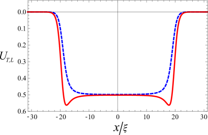
Figure 1: One-dimensional potential wells $U_{T}$ (blue dashed) and $U_{L}$ (red solid) for $s=0.5$ and $E=0.01$.

When the spectrum of the Schröedinger operator is known analytically the zero mode can be explicitly excluded from the product of eigenvalues. Therefore, the determinant can be calculated simply as an infinite product of non-zero eigenvalues. This is illustrated in Appendix C.1 for the fluctuation operators $M_{T}$ and $M_{L}$ arising in the Gaussian disorder model Cardy78 . For the blue detuned speckle the determinants of $M_{T}$ and $M_{L}$ cannot be calculated simply as a product of non-zero eigenvalues because the spectrum cannot be found analytically. Fortunately, Gel’fand and Yaglom (GY) Gelfand60 ; Kleinert04 derived long ago a general formula which allows one to calculate the functional determinant of a Schrödinger like operator at least in one dimension without knowing any of its eigenvalues. The GY method can be applied to an operator of the form

$${\cal M}=-\frac{d^{2}}{dx^{2}}+U(x)+m^{2},$$ (28)

which is defined on $x\in[-L,L]$ for the wave functions satisfying the boundary conditions $u(-L)=u(L)=0$. The limit $L\to\infty$ can be taken at the end of the calculation. Since the well defined object is rather a ratio of two determinants than a single functional determinant itself it is convenient to introduce a free operator ${\cal M}_{\rm free}=-\frac{d^{2}}{dx^{2}}+m^{2}$. The GY theorem Gelfand60 states that

$$\frac{\det{\cal M}}{\det{\cal M}_{\rm free}}=\frac{u(L)}{u_{\rm free}(L)},$$ (29)

where $u(x)$ and $u_{\rm free}(x)$ are the solutions of the Cauchy problems

$${\cal M}u(x)=0\hskip 14.22636pt\mathrm{and}\hskip 14.22636pt{\cal M}_{\rm free}u_{\rm free}(x)=0$$ (30)

with the initial conditions:

$$u(-L)=u_{\rm free}(-L)=0,\ \ \ u^{\prime}(-L)=u_{\rm free}^{\prime}(-L)=1.$$

Due to the presence of eigenfunctions with zero eigenvalue, whose contributions to the determinant have to be excluded, the GY formula (29) has to be slightly modified for the operators $M_{T}$ and $M_{L}$. A simple regularization consists of introducing an infinitesimal shift of the spectrum by a small shift of the mass $m$. Then, the original determinant with the excluded zero mode can be derived by differentiating with respect to the mass. This method is illustrated for the operators $M_{T}$ and $M_{L}$ of the Gaussian disorder model in Appendix C.2.

In the case of the speckle potential it turns out to be more convenient to use another regularization approach which has been recently proposed by Tarlie and McKane (TM) in Ref. Tarlie95 . It is based on the GY method generalized to an arbitrary boundary conditions by Forman in Ref. Forman87 . The basic idea is to regularize the determinant by modifying the boundary conditions. This changes the zero eigenvalue to a nonzero one which can be estimated to lowest order in the difference between the original and regularized boundary conditions. Assuming that the zero mode of the operator $\mathcal{M}$ is given by $v_{0}(x)$ the ratio of the two determinants with excluded zero mode can be written as

$$\frac{\det^{\prime}\mathcal{M}}{\det\mathcal{M}_{\rm free}}=-\frac{\left\langle v_{0}|v_{0}\right\rangle}{v_{0}^{\prime}(-L)v_{0}^{\prime}(L)}\frac{u^{\prime}_{\rm free}(-L)}{u_{\rm free}(L)},$$ (32)

where we defined the scalar product

$$\left\langle v_{0}|v_{0}\right\rangle:=\int_{-L}^{L}dx\,v_{0}^{2}(x).$$ (33)

The TM formula is very useful because the zero mode of the operator $M_{T}$ is given by the classical solution $\phi_{0}(x)$ while for the operator $M_{L}$ the zero mode is simply given by its derivative $\phi_{0}^{\prime}(x)$. This is true not only in the case of the one dimensional speckle potential but also for the problem with uncorrelated Gaussian disorder where the TM formula is shown to reproduce the correct result of Cardy (see Appendix C.3). By inserting the zero mode solutions in Eq. (32) the ratio of the two determinants $M_{T}$ and $M_{L}$ of Eq. (27) in one dimension can be rewritten as

$$\frac{\det^{\prime}M_{T}}{\det^{\prime}M_{L}}=\lim_{L\rightarrow\infty}\frac{\left\langle\phi_{0}|\phi_{0}\right\rangle}{\left\langle\phi^{\prime}_{0}|\phi^{\prime}_{0}\right\rangle}\frac{\phi^{\prime\prime}_{0}(-L)\phi^{\prime\prime}_{0}(L)}{\phi^{\prime}_{0}(-L)\phi^{\prime}_{0}(L)},$$ (34)

because the contribution from the free operator cancels out. Moreover, in one dimension, the derivatives of the classical solution can be easily obtained from the first order differential equation (18) derived from the analogy with the particle in a conservative potential. Although the function $\phi_{0}(x)$ is known only numerically, the limit of Eq. (34) can be calculated analytically by using that this solution is regular at infinity. We find the exact relation

$$\frac{\det^{\prime}M_{T}}{\det^{\prime}M_{L}}=-\frac{\left\langle\phi_{0}|\phi_{0}\right\rangle}{\left\langle\phi^{\prime}_{0}|\phi^{\prime}_{0}\right\rangle}\left(s-\tilde{E}\right).$$ (35)

When we substitute this result in the DOS (25) the ratio of two scalar products in Eq. (35) cancel exactly the Jacobian (26). Using the saddle point solution (15) in the asymptotic limit $E\rightarrow 0$ we obtain

$$\mathcal{A}_{1}\sim\frac{\ln{\left({s}/\tilde{E}\right)}}{\tilde{E}^{3/2}}{s}^{1/2}.$$ (36)

By collecting all contributions, we find the tail of the DOS in one dimension

$$\nu=\frac{A}{\xi I_{0}}\left(\frac{I_{0}}{E}\right)^{3/2}\ln\left(\frac{I_{0}}{E}\right)\exp\left[-\pi s^{-1/2}\sqrt{\frac{I_{0}}{E}}f_{1}\left(\frac{I_{0}}{E}\right)\right],$$

where $A$ is a numerical constant and

$$f_{1}(y)=\frac{2}{\pi}\int\limits_{0}^{z_{0}}dz\sqrt{z^{-1}\ln(1+yz)-1},$$ (38)

whose asymptotics for large $y$ is $f_{1}(y)=\ln y$.

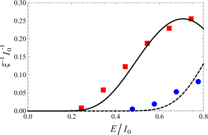
Figure 2: The one particle DOS for a blue-detuned speckle potential computed numerically for $s=1$ (red squares) and $s=0.1$ (blue circles). The solid and dashed lines are the best fit of the tails by Eq. (IV.1).

In order to check this formula we have fitted the low energy tail of the DOS in 1D speckle potential which we computed numerically using the exact Hamiltonian diagonalization in Ref. Giacomelli10 . The result is shown in Fig. 2.

IV.2 Higher dimensions

The GY method can be extended to determinants of the Schrödinger-like operators in $d$ dimensions in the case of radially symmetric potentials Kirsten06 . Due to the radial symmetry of the operators, their eigenfunctions can be decomposed into a product of radial parts and hyperspherical harmonics

$$\Psi\left(r,{\mathbf{\vartheta}}\right)=\frac{1}{r^{\frac{d-1}{2}}}\psi_{\ell}(r)~{}Y_{\ell}(\vartheta).$$ (39)

The radial parts $\psi_{\ell}(r)$ are then solutions to the radial equations

$${M}_{T,L}^{(\ell)} ~{}\psi_{\ell}(r):=\left(-\frac{d^{2}}{dr^{2}}+\frac{\left(\ell+\frac{d-3}{2}\right)\left(\ell+\frac{d-1}{2}\right)}{r^{2}}+\right.$$ (40)

$$\left.+U_{T,L}(r)+m^{2}\right){\psi_{\ell}(r)}=\lambda~{}\psi_{\ell}(r).\$$

The radial eigenfunctions $\psi_{\ell}(r)$ come with a degeneracy factor of

$${\rm deg}\left(\ell;d\right)=\frac{(2\ell+d-2)(\ell+d-3)!}{\ell!(d-2)!}.$$ (41)

The determinant of a radially separable operator can be calculated by combining the determinants for each partial wave $\ell$ with the weights given by the degeneracy factor (41) as follows

$$\ln{\frac{\det^{\prime}{M}_{T,L}}{\det{M}_{\rm free}}}=\sum_{\ell=0}^{\infty}{\rm deg}\left(\ell;d\right)~{}\ln{\frac{\det^{\prime}{M}_{T,L}^{(\ell)}}{\det{M}_{\rm free}^{(\ell)}}},$$ (42)

where the free operators have been defined as

$${M}_{\rm free}^{(\ell)}=-\frac{d^{2}}{dr^{2}}+\frac{\left(\ell+\frac{d-3}{2}\right)\left(\ell+\frac{d-1}{2}\right)}{r^{2}}+m^{2}.$$ (43)

In order to compute the determinants of the partial operators in Eq. (42) one can use the GY method for those determinants that have no zero modes and the MT method for those that have them. The only partial operators which have zero modes are ${M}_{T}^{(0)}$ and ${M}_{L}^{(1)}$. All other determinants can be computed using the GY formula

$$\frac{\det{M}_{T,L}^{(\ell)}}{\det{M}_{\rm free}^{(\ell)}}=\lim_{R\rightarrow\infty}\frac{u^{(\ell)}(R)}{u_{\rm free}^{(\ell)}(R)},$$ (44)

where $u^{(\ell)}$ and $u_{\rm free}^{(\ell)}$ are the solution of the following Cauchy problems

$${M}^{(\ell)}u^{(\ell)}(r)=0,\hskip 8.53581ptu^{(\ell)}\sim r^{\ell+\frac{(d-1)}{2}},\hskip 8.53581ptr\rightarrow 0,$$ (45)

$${M}^{(\ell)}_{\rm free}u^{(\ell)}_{\rm free}(r)=0,\hskip 8.53581ptu_{\rm free}^{(\ell)}\sim r^{\ell+\frac{(d-1)}{2}},\hskip 8.53581ptr\rightarrow 0.\ \ \ \ \$$ (46)

The determinants of the operators ${M}_{T}^{(0)}$ and ${M}_{L}^{(1)}$ with excluded zero modes are given by the generalization of Eq. (32) which reads

$$\frac{\det^{\prime}\mathcal{M}}{\det\mathcal{M}_{\rm free}}=-\lim\limits_{R\to\infty}\frac{\left\langle v_{0}|v_{0}\right\rangle}{v_{0}^{\prime}(R)u_{\rm free}(R)}.$$ (47)

Here we have used that the zero modes $v_{0}(r)$ of the operators ${M}_{T}^{(0)}$ and ${M}_{L}^{(1)}$ and the solution $u_{\rm free}(r)$ of the Cauchy problem (46) have the same behavior at $r\to 0$.

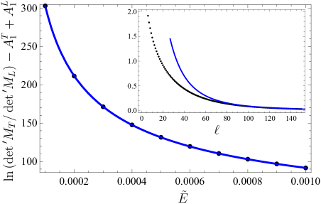
Figure 3: The logarithm of the ratio of determinants $M_{T}$ and $M_{L}$ with subtracted diagrams $A^{T,L}_{1}$ computed numerically for $s=0.5$ and $d=2$ as a function of $\tilde{E}$ using Eq. (LABEL:eq:sum-finite). The solid blue line is a fit by ${3.18156}/\sqrt{\tilde{E}}+2.82111\ln\tilde{E}+10.5708$. (Inset) The logarithm of the ratio of partial determinants for $d=2$, $\tilde{E}=0.0005$, and $s=0.5$ as a function of $\ell$. The solid blue line is the asymptotic behavior ${162085}/{(\ell+21.4092)^{3}}$.

It turns out that the sum over $\ell$ in Eq. (42) diverges for $d\geq 2$ as $1/\ell$. This divergence is a general property of functional determinants in $d\geq 2$ Dunne08 that was not discussed in the most works on the instanton approach to the DOS of disordered systems Cardy78 ; John84 ; Luttinger83 ; yaida12 . This divergence reflects the fact that the field theory (11) has to be renormalized bresin1980 that is beyond the scope of the present paper. To make the theory finite we introduce the UV cutoff $\Lambda$ and separate the divergencies from the sum over $\ell$ in Eq. (42). Following Ref. Kirsten06 we use the diagrammatic representation of the determinants ${M}_{T,L}$ explained in Appendix A and given by Eq. (56) with $V(r)=U_{T,L}(r)$. For $2\leq d<4$ the only divergent diagram is $A_{1}$ which is linear in $V$. For $d=4$ one has also subtract the diagram $A_{2}$ which is quadratic in $V$. Subtracting the divergent diagram from the partial determinants we obtain

$$\ln\frac{\det^{\prime}{M}_{T,L}}{\det{M}_{\rm free}} = A_{1}+\sum_{\ell=0}^{\infty}{\rm deg}(\ell;d)\,\left[\ln\frac{\det^{\prime}{M}^{(\ell)}_{T,L}}{\det{M}^{(\ell)}_{\rm free}}\right]_{\emptyset(V)},$$

where the symbol $\left[...\right]_{\emptyset(V)}$ means that the parts of order $V$ have been subtracted. The sum over $\ell$ in Eq. (LABEL:eq:sum-finite) becomes finite because the UV divergences have been accumulated in the regularized Feynman diagram $A_{1}$. The explicit form of the terms which have to be subtracted for a general potential $V(x)$ is given by the expansion Kirsten06

$$\ln\frac{\det\mathcal{M}^{(\ell)}}{\det\mathcal{M}^{(\ell)}_{\rm free}} = \int\limits_{0}^{\infty}dr\,r\,V(r)K_{\nu}(mr)I_{\nu}(mr)$$ (49)

$$-\int\limits_{0}^{\infty}dr\,r\,V(r)K_{\nu}^{2}(mr)\int\limits_{0}^{r}dr^{\prime}\,r^{\prime}\,$$

$$\times V(r^{\prime})I_{\nu}^{2}(mr^{\prime})+{\cal O}(V^{3})\quad,$$

where $I_{\nu}$ and $K_{\nu}$ are the Bessel function with $\nu\equiv l+\frac{d}{2}-1$. Thus, one can compute the regularized ratio of the functional determinants (LABEL:eq:sum-finite) by solving numerically the Cauchy problems (45)-(46) and using the GY and MT formulas (44) and (47). We have found that after subtracting the diverging term given by the first line in Eq. (49) the sum over $\ell$ in Eq. (LABEL:eq:sum-finite) converges asymptotically as $1/\ell^{3}$ in $d=2$ and as $1/\ell^{2}$ in $d=3$. As an example, this sum is shown as a function of $\tilde{E}$ for $d=2$ and $s=0.5$ in Fig. 3. The total ratio of the determinants, however, is dominated by the exponential of

$$A_{1}^{T}-A_{1}^{L}=\int_{q}\frac{1}{q^{2}+m^{2}}\int d^{d}x[U_{T}(x)-U_{L}(x)].$$ (50)

Neglecting a power-law correction resulting from the Jacobian (26) we arrive at

$$\mathcal{A}_{d}(E)\sim\exp\left[\gamma_{d}\left(\frac{I_{0}/E}{\ln(I_{0}/{E})}\right)^{(d-1)/2}\right]$$ (51)

with UV cutoff-dependent coefficients $\gamma_{2}=1.89\ln({\Lambda}/{s})$ and $\gamma_{3}=14.81\Lambda$.

V Weakly interacting Bose gas in speckle potential

We now consider the effect of weak repulsive interaction on the bosons in the Lifshitz tail. We restrict our consideration to the three dimensional system in dilute regime. The corresponding Hamiltonian has the well-known form Falco09-2

$$H = \int d^{3}x\psi^{\dagger}(x)\left(-\frac{\hbar^{2}}{2m_{0}}\nabla^{2}+V(x)-\mu\right)\psi(x)$$ (52)

$$\ \ \ \ \ +\,\frac{g}{2}\int d^{d}x(\psi^{\dagger}(x)\psi(x))^{2},$$

where $\psi(x)$ is the secondary quantized wave function, $V(x)$ - random potential and $\mu$ - the chemical potential. The positive coupling constant is given by $g=4\pi\hbar^{2}a_{s}/m_{0}$, where $a$ is the scattering length and we assume a low concentration of bosons $n$, such that $na_{s}^{3}\ll 1$. The aim is to find how the bosons fill the random potential when we add the particles one by one. In particular, we are interested in the dependence of the chemical potential on the density of bosons. It is instructive to compare the case of a bounded from below potential with the random uncorrelated Gaussian potential studied by one of us in Ref. Falco09-2 .

In the case of Gaussian disorder the asymptotic behavior of the DOS for large negative energy $E$ is dominated by the optimal wells of width $R$ with the energy $E_{0}(R)=-\hbar^{2}/(2m_{0}R^{2})$ which decreases with shrinking of $R$. The density of optimal wells, which can be found from the corresponding instanton solution, is $n_{w}(R)\sim e^{-\mathcal{L}/R}/R^{3}$, where $\mathcal{L}=\hbar^{4}/(m_{0}^{2}\gamma^{2})$ is the so-called Larkin length related to the strength of disorder $\gamma$ Falco09-2 . In the presence of weak repulsive interactions the positive repulsion energy per particle grows with decreasing $R$ as $E_{r}(R)=3g\mathcal{N}(R)/(4\pi R^{3})$, where $\mathcal{N}(R)=n/n_{w}(R)$ is the typical number of bosons in optimal wells. Since the both energies $E_{0}(R)$ and $E_{r}(R)$ have opposite behavior with respect to decreasing $R$ one has to optimize the total energy in order to find the size of the optimal well renormalized by interactions. This yields with the logarithmic precision $R(n)=\mathcal{L}/\ln(n_{c}/n)$. Then the relation between the chemical potential and the density is given by Falco09-2

$$\mu(n)=-\frac{\hbar^{2}}{2m_{0}R^{2}(n)}\approx-\frac{\mathcal{E}}{2}\left(\ln\frac{n_{c}}{n}\right)^{2},$$ (53)

where $\mathcal{E}=\hbar^{2}/(m_{0}\mathcal{L}^{2})$ and $n_{c}=(3\mathcal{L}^{2}a_{s})^{-1}$.

In the case of the speckle potential both the energy corresponding to the optimal well $E_{0}(R)=\hbar^{2}/(2m_{0}R^{2})$ and the positive repulsion energy decay with growing the size of the typical well. Thus, there is no competition between the disorder and interactions so that we have no need for optimization of the total energy. Neglecting the kinetic energy and using Eq. (16) to estimate the density of the optimal wells we obtain with the logarithmic precision

$$\mu(n)\approx E_{\xi}\left(v_{3}\ln\frac{I_{0}}{E_{\xi}}\right)^{2/3}\,\left(\ln\frac{n_{0}}{n}\right)^{-2/3},$$ (54)

where $n_{0}=(6\xi^{2}a_{s})^{-1}$ and $v_{3}=4\pi^{4}/3$. The asymptotic behavior (54) holds for $n\ll n_{0}$ and $E_{\xi}\ll I_{0}$ and is an agreement with Ref. Gopalakrishnan12 .

VI Conclusion

We have studied the low energy behavior of the DOS for non-interacting bosons in a $d$ dimensional blue detuned laser speckle potential. We have shown that for $E\leq E_{\xi}$ the precise form of the electric field correlator does not affect the asymptotic behavior. Using an instanton approach we have found the saddle point solution which gives the leading exponential behavior. Integrating out the Gaussian fluctuation around this solution we have expressed the prefactor in the form of ratio of two functional determinants. In one dimension we calculated the ratio of functional determinants exactly using the generalized GY method which allows one to take into account not only the discrete part of the spectrum of fluctuation operators but also the continuous one. In higher dimensions the corresponding ratio diverges that has been overlooked in most of the previous work on the instanton approach to the DOS of disordered systems. Using the partial wave decomposition we can separate the UV divergences to a regularized one-loop Feynman diagram and obtain a finite result for the DOS tail in $d>1$. In Appendix C.4 we show that this method gives a correct result for the case of Gaussian uncorrelated disorder. We also discussed the effect of weak repulsion interactions in the DOS tail. In contrast to the Gaussian unbounded disorder the interactions and disorder do not compete and the optimal wells are not renormalized by interactions that leads to a different dependence of the chemical potential on the bosons density.

Appendix A Functional determinant representation

The diagrams in Eq. (56) can not be summed up for an arbitrary distribution of the electric fields including those that appear in real experiments. In this appendix we show that the sum can be performed for a special choice of the Gaussian distribution of the electric fields with zero mean and variance

$$G(x)=I_{0}\frac{2^{d/2}}{\Gamma\left(1-\frac{d}{2}\right)}\left(\frac{x}{\xi}\right)^{1-\frac{d}{2}}K_{d/2-1}\left(\frac{x}{\xi}\right),$$ (55)

where $K_{\nu}(x)$ is the modified Bessel function. A similar correlator appears in the problem of the Bragg glass studied in Ref. Fedorenko14 . For $d=1$ the variance (55) reduces to $G(x)=I_{0}\ e^{-|x|/\xi}$. This is particular interesting because the asymptotic behavior of the DOS does not depend on the precise form of correlations in disorder but it is determined by the lower energy states which spread over distances larger than the disorder correlation length $\xi$. Therefore, in order to study the lowest order corrections to the asymptotic tail due to presence of correlations one can use Eq. (55) as a reasonable approximation for the variance of the electric field.

The starting point is the following diagrammatic representation of the ratio of two functional determinants

$$\ln\left(\frac{\det(-\nabla^{2}+V(x)+m^{2})}{\det(-\nabla^{2}+m^{2})}\right)=\sum\limits_{n=1}^{\infty}\frac{(-1)^{n+1}}{n}A_{n}$$

$$\mbox{}\hskip 28.45274pt=\parbox{22.76219pt}{\includegraphics[width=22.76219pt]{diag1}}-\frac{1}{2}\parbox{22.76219pt}{\includegraphics[width=22.76219pt]{diag2}}+\frac{1}{3}\parbox{22.76219pt}{\includegraphics[width=22.76219pt]{diag3}}-...$$ (56)

In the diagrams shown in Eq. (56) the dots correspond to the potential $V(x)$ and the lines stand for the Green’s function

$$C_{0}(x)=\frac{m^{d-2}}{(2\pi)^{d/2}}\frac{K_{d/2-1}(m|x|)}{(m|x|)^{d/2-1}},$$ (57)

which satisfies the equation

$$\left[-\nabla^{2}+m^{2}\right]C_{0}(x)=\delta(x).$$ (58)

If we separate the combinatorial factors from the diagrams in Eq. (8) we obtain the same series as in Eq. (56). Thus, one can formally rewrite the sum of the diagrams in Eq. (8) as a ratio of two functional determinants with the mass $m=1/\xi$ and the potential $V(x)=\frac{1}{2}I_{0}\bar{\phi}^{2}(x)/C_{0}(0)$ resulting from a random Gaussian electric field with zero mean and variance $G(x)=I_{0}C_{0}(x)/C_{0}(0)$. Note that divergency of $C_{0}(0)$ when $d\geq 2$ reflects the fact that the functional determinants in Eq. (56) require a renormalization for $d\geq 2$. Here we restrict ourselves to the case $d=1$ and obtain

$$\!\!\!\!\!\!S(E)=\int dx\left[\frac{\hbar^{2}}{4m_{0}^{2}}(\nabla\bar{\phi}(x))^{2}-\frac{1}{2}E\bar{\phi}^{2}(x)\right]$$

$$\ \ \ +\ln\left(\frac{\det(-\nabla^{2}+\left(I_{0}/\xi\right)\bar{\phi}^{2}(x)+1/\xi^{2})}{\det(-\nabla^{2}+1/\xi^{2})}\right).$$ (59)

In the limit $\xi\to 0$ we can neglect the $\nabla^{2}$-operator in the determinants of Eq. (59) and recover Eq. (10) using that $\ln\det=\mathrm{Tr}\ln$. The corresponding saddle point equation

$$\frac{\hbar^{2}}{2m_{0}^{2}}\nabla^{2}\bar{\phi}(x) + E\bar{\phi}(x)=\frac{\delta}{\delta\bar{\phi}(x)}\ln\det\left[-\nabla^{2}\right.$$ (60)

$$\left.+\left(I_{0}/\xi\right)\bar{\phi}^{2}(x)+1/\xi^{2}\right]$$

has the form of a gap equation known in relativistic quantum field theory Dunne08 .

Appendix B Variational method with Gaussian trial functions

One can also sum up all diagrams in Eq. (8) for a particular class of functions $\bar{\phi}(x)$ that can be used to find variationally an approximative instanton solution by means of the trial function method. Let us assume that the one dimensional electric field correlator has the form

$$G(x-y)=I_{0}\xi\delta_{\xi}(x-y)\hskip 5.69054pt\mathrm{with}\hskip 5.69054pt\delta_{\xi}(x)=\frac{1}{\xi}e^{-\pi x^{2}/\xi^{2}}.$$ (61)

For the trial function we consider $\phi(x)=\bar{n}\phi_{0}(x)$ with $\bar{n}^{2}=1$ and

$$\phi_{0}(x)=\sqrt{C}e^{-\pi x^{2}/2a^{2}}.$$ (62)

By substituting the trial function into the potential part of the action (8) we find that the diagram with $n$ electric field correlators reads

$$= (n-1)!\,I_{0}^{n}\,C^{n}\int dx_{1}...dx_{n}\exp\left[-\frac{\pi x_{1}^{2}}{a^{2}}\right.$$ (63)

$$-\frac{\pi(x_{1}-x_{2})^{2}}{\xi^{2}}...-\frac{\pi(x_{n-1}-x_{n})^{2}}{\xi^{2}}$$

$$\left.-\frac{\pi x_{n}^{2}}{a^{2}}-\frac{\pi(x_{n}-x_{1})^{2}}{\xi^{2}}\right].$$

Upon making the variable rescaling $x_{i}\to\xi x_{i}/\pi$, the integral in Eq. (63) can be rewritten as

$$\frac{\xi^{n}}{\pi^{n}}\int dx_{1}...dx_{n}\exp\left[-\sum\limits_{i,j=1}^{n}x_{i}A_{ij}x_{j}\right]=\frac{\xi^{n}}{\pi^{n/2}}[\det A_{n}]^{-1/2},$$

where we have introduced the matrix

$$A_{n}=\left(\begin{array}[]{cccccc}2+\epsilon^{2}&-1&0&...&0&-1\\ -1&2+\epsilon^{2}&-1&...&0&0\\ 0&-1&2+\epsilon^{2}&...&0&0\\ ...&...&...&...&...&...\\ 0&0&0&...&2+\epsilon^{2}&-1\\ -1&0&0&...&-1&2+\epsilon^{2}\\ \end{array}\right),$$ (71)

with $\epsilon=\xi/a$. The determinant of $A_{n}$ can then be calculated, and we get

$$\det A_{n} = \sum\limits_{m=0}^{n-1}\frac{\prod_{i=0}^{m}(n^{2}-i^{2})}{2^{m}(2m+1)!!(m+1)!}\epsilon^{2+2m}$$ (72)

$$=4\sinh^{2}\left[n~{}\mathrm{arcsinh}\frac{\epsilon}{2}\right].$$

Therefore, the action evaluated using the trial function (62) can be written as

$$S(E) = \int dx\left[\frac{\hbar^{2}}{4m_{0}}(\phi_{0}^{\prime\prime}(x))^{2}-\frac{1}{2}E{\phi}_{0}^{2}(x)\right]$$ (73)

$$- \sum\limits_{n=1}^{\infty}\frac{(-1)^{n}}{2n}\frac{(I_{0}\xi C)^{n}}{(\sqrt{\pi})^{n}}\frac{1}{\sinh\left[n~{}\mathrm{arcsinh}\frac{\epsilon}{2}\right]}.$$

When $E\sim 1/{a^{2}}\ll E_{\xi}=1/{\left(2\xi^{2}\right)}$ we can approximate $\sinh\left[n~{}\mathrm{arcsinh}\frac{\epsilon}{2}\right]\approx n\epsilon/2$. As a result the second line of Eq. (73) is simplified to $-\mathrm{Li}_{2}[-I_{0}\xi C/\sqrt{\pi}]/\epsilon$. This expression can be also derived by applying the trial function method directly to the action (10). This means that the action (10) obtained in the limit of uncorrelated speckle potential properly describes the DOS in the presence of correlations for $E\ll E_{\xi}$. For these low laying states the finite range correlations play no role because the typical width of the wave functions $a$ is much larger than the correlation length of disorder $\xi$.

Appendix C The Lifshitz tail for a particle in Gaussian uncorrelated disorder

In order to illustrate the power of the GY and MT methods, we reconsider here the problem of a particle in uncorrelated Gaussian disorder. There existed a disagreement in the literature on the preexponential factor in the asymptotic behavior of the DOS in the tail of the band Cardy78 ; Zittartz1966 ; yaida12 . The two points that have not been sufficiently discussed in these works are the contribution of the continuous part of the spectrum to the functional determinants and divergence of functional determinants in $d\geq 2$ Houghtont79 . The replicated action of the system is given by Cardy78

$$S_{\rm av}=\int d^{d}x \left\{\frac{1}{2}(\nabla\bar{\phi}(x))^{2}-\frac{1}{2}E\bar{\phi}^{2}(x)-\frac{1}{6}(\gamma/4)^{2}(\bar{\phi}(x))^{2}\right\}$$

and we look for the asymptotic behavior of the DOS in the limit $E\to-\infty$. The saddle point solution to the action (C) has the form

$$\bar{\phi}_{\rm cl}=\frac{(-E)^{1/2}}{\gamma}f(\sqrt{-E}x)~{}\bar{n},$$ (75)

where $f$ satisfies the dimensionless equation of motion

$$\nabla^{2}f-f=-\frac{f^{3}}{24}.$$ (76)

The action (C) evaluated at the saddle point behaves as $S_{\rm cl}\sim(-E)^{2-d/2}/\gamma^{2}$. By repeating the calculations (25)-(27) we find the DOS tail

$$\nu(E)\sim(-E)^{1/2-d^{2}/4+3d/4}\sqrt{\frac{\det^{\prime}M_{\mathrm{T}}}{\det^{\prime}M_{\mathrm{L}}}}~{}e^{-S_{\rm cl}},$$ (77)

where the regularized determinants of the fluctuation operators need to be calculated. The transverse and longitudinal operators derived by expansion around the saddle point solution have the form

$$M_{\mathrm{T}}=-{\nabla}^{2}-E\left[1-\frac{1}{24}f\left(\sqrt{-E}x\right)^{2}\right]$$ (78)

$$M_{\mathrm{L}}=-{\nabla}^{2}-E\left[1-\frac{1}{8}f\left(\sqrt{-E}x\right)^{2}\right],$$ (79)

where the energy $E$ is assumed to be large and negative.

C.1 Brute force method in $d=1$

The one dimensional case is interesting for testing the GY method because the ratio of determinants of the operators (78) and (79) can also be calculated directly from the product of their eigenvalues. The saddle point solution of Eq. (76) is

$${}f(x)=4\sqrt{3}~{}{\rm sech}(x)$$ (80)

and the operators (78)-(79) can be rewritten in the form of Pöschl-Teller operators Kleinert04 ; Dunne08

$${\cal M}_{m,j}=-\frac{\partial^{2}}{\partial x^{2}}+|E|~{}\left[m^{2}-j\left(j+1\right){{\rm sech^{2}}{\left(\sqrt{-E}~{}x\right)}}\right],$$

where $j$ takes integer values. The operators (78) and (79) correspond to the case $M_{T}={\cal{M}}_{1,1}$ and $M_{L}={\cal{M}}_{1,2}$. The spectrum of the Pöschl-Teller operator ${\cal M}_{m,j}$ contains a discrete part which have $j$ bound states $\varepsilon_{\ell}=|E|\left(m^{2}-\ell^{2}\right)$ ($\ell=1,...,j$) and the continuous part $\varepsilon(k)=|E|\left(k^{2}+m^{2}\right)$ with the density of states

$$\nu_{j}\left(k\right)=\frac{L}{2\pi}-\frac{1}{\pi}\sum_{\ell=1}^{j}{\frac{\ell}{\ell^{2}+k^{2}}},$$ (82)

which has been regularized by putting the system in a box of size $L$. This yields

$$\!\!\log\frac{\det{{\cal{M}}_{m,j}}}{\det{{\cal{M}}_{m,0}}}=\sum_{\ell=1}^{j}{\log{\left[|E|\left(m^{2}-\ell^{2}\right)\right]}}$$

$$\ \ \ \ +\int^{\infty}_{-\infty}dk~{}\nu_{j}\left(k\right)\log{\left[|E|~{}\left(k^{2}+m^{2}\right)\right]},$$ (83)

where the free particle contribution $L/2\pi$ has been canceled. From this formula the functional determinants of the operators (78)-(79) can be determined straightforwardly. The operator $M_{T}={\cal{M}}_{1,1}$ has just one discrete zero eigenvalue. Excluding this zero mode, the only contribution comes from the continuous spectrum given by the second line in Eq. (C.1),

$$\frac{\det{{{{}^{\prime}{M}}}_{T}}}{\det M_{\rm free}}=\frac{1}{4|E|},$$ (84)

where $M_{\rm free}:={\cal{M}}_{m,0}$. The operator $M_{L}={{M}}_{1,2}$ has two discrete eigenvalues: a negative eigenvalue ($\ell=2$) giving a finite imaginary part of the Green function (4), and a zero eigenvalue ($\ell={1}$). The negative mode and the continuous spectrum contribute with

$$\frac{\det{{{{}^{\prime}{M}}}_{L}}}{\det M_{\rm free}}=-\frac{1}{12|E|}.$$ (85)

We obtain

$$\lim_{N\rightarrow 0}\det{{}^{\prime}M_{L}}^{-1/2}\cdot\det{{}^{\prime}M_{T}}^{-(N-1)/2}=i~{}\sqrt{3},$$ (86)

which is independent of $E$.

C.2 Regularized Gel’fand-Yaglom formula

The same result can also be obtained using the GY method (29). The solution $u_{m,j}$ of the corresponding Cauchy problem (30)-(IV.1) for the Pöschl-Teller operators ${\cal M}_{m,j}$ (C.1) can be found analytically. For the sake of compactness, we show here the formula for $|E|=1$,

$$u_{m,j}(L)=\frac{1}{\left(1+j-m\right)}$$

$$\times\frac{-P^{m}_{j}\left(Y\right)Q^{m}_{j}\left(-Y\right)+P^{m}_{j}\left(-Y\right)Q^{m}_{j}\left(Y\right)}{P^{m}_{j+1}\left(-Y\right)Q^{m}_{j}\left(-Y\right)-P^{m}_{j}\left(-Y\right)Q^{m}_{j+1}\left(-Y\right)},$$

where we defined $Y:=\tanh L$ and $P^{m}_{j}(x)$ and $Q^{m}_{j}(x)$ are the Legendre functions. The solution (C.2) for the free operator ${\cal M}_{\rm free}={\cal M}_{m,0}$ reduces to

$$u_{m,0}(L)=\frac{\sinh{\left[2mL\right]}}{m}.$$ (88)

The ratio of the two determinants is then given by

$$\frac{\det{\cal M}_{m,j}}{\det{\cal M}_{m,0}}=\lim\limits_{L\to\infty}\frac{u_{m,j}(L)}{u_{m,0}(L)}.$$ (89)

In order to exclude the zero modes, we apply a shift of the mass $m\rightarrow\sqrt{m^{2}+\delta m^{2}}$ that gives

$$\frac{\det\left({\cal M}_{m,j}+\delta m^{2}\right)}{\det\left({\cal M}_{m,0}+\delta m^{2}\right)}\sim\delta m^{2}\frac{\det{{}^{\prime}\cal M}_{m,j}}{\det{\cal M}_{{m,0}}},\hskip 5.69054pt\delta m^{2}\rightarrow 0.\$$

Restoring the dependence on $E$ we obtain

$$\frac{\det{{}^{\prime}\cal M}_{1,j}}{\det{\cal M}_{{1,0}}}=(-1)^{j+1}\frac{1}{2j(j+1)|E|}$$ (90)

in agreement with Eq. (84)-(85) for $j=1$ and $j=2$ respectively.

C.3 McKane-Tarlie formula

We now apply the MT method. First, we need the zero modes of the operators $M_{T}={\cal M}_{1,1}$ and $M_{L}={\cal M}_{1,2}$. They are given by $v_{1,1}(x)=|E|f(\sqrt{-E}x)$ and $v_{1,2}(x)=|E|^{3/2}f^{\prime}(\sqrt{-E}x)$, respectively. Then, according to Eq. (34), the ratio of the determinants with excluded zero modes is given by

$$\frac{\det^{\prime}M_{T}}{\det^{\prime}M_{L}}=\lim_{L\rightarrow\infty}\frac{\left\langle v_{1,1}|v_{1,1}\right\rangle}{\left\langle v_{1,2}|v_{1,2}\right\rangle}\frac{v_{1,2}^{\prime}(-L)v_{1,2}^{\prime}(L)}{v_{1,1}^{\prime}(-L)v_{1,1}^{\prime}(L)}=-3,$$

where we used

$$\left\langle v_{1,1}|v_{1,1}\right\rangle=2|E|^{3/2},$$ (92)

$$\left\langle v_{1,2}|v_{1,2}\right\rangle=\frac{2}{3}|E|^{5/2},$$ (93)

$$\frac{v_{1,2}^{\prime}(-\infty)}{v_{1,1}^{\prime}(-\infty)}=-\frac{v_{1,2}^{\prime}(\infty)}{v_{1,1}^{\prime}(\infty)}=\sqrt{-E}.$$ (94)

C.4 Gel’fand-Yaglom method generalized to radial operators for $d>1$

The radial parts of the eigenfunctions of the operators (78) and (79) satisfy Eq. (40) with the mass $m=|E|$ and the potentials

$$U_{T}(r)=-\frac{|E|}{24}f\left(\sqrt{-E}r\right)^{2},$$ (95)

$$U_{L}(r)=-\frac{|E|}{8}f\left(\sqrt{-E}r\right)^{2}.$$ (96)

Scaling analysis shows that the solutions of the corresponding Cauchy problems (45) and (46) have the form

$$u^{(\ell)} = |E|g^{(\ell)}(|E|^{1/2}r),$$ (97)

$$u^{(\ell)}_{\rm free} = |E|g^{(\ell)}_{\rm free}(|E|^{1/2}r).$$ (98)

There is no zero modes for $\ell>1$ and we can apply the GY formula (44). The ratio of the partial determinants for $\ell>1$ is given by

$$\lim_{R\to\infty}g^{(\ell)}(|E|^{1/2}R)/g^{(\ell)}_{\rm free}(|E|^{1/2}R),$$ (99)

which does not depend on $E$. Thus, all the ratios of the partial determinants with $\ell>1$ do not contribute to the $E$ dependance of the full ratio of the functional determinants.

The operators ${M}_{T}^{(0)}$ and ${M}_{L}^{(1)}$ have a zero eigenvalue so that to exclude it we apply the MT method. The corresponding ratios of the partial determinants can be calculated using Eq. (47). The scaling behavior of the zero mode eigenfunction $v_{0}(r)$ is again given by

$$v_{0}(r)=|E|g_{0}(|E|^{1/2}r).$$ (100)

This yields

$$\left\langle v_{0}|v_{0}\right\rangle\sim|E|^{3/2},$$ (101)

$$\lim_{R\to\infty}v_{0}^{\prime}(R)u_{\rm free}(R)=|E|^{5/2}\lim_{R\to\infty}g_{0}^{\prime}(R)g_{\rm free}(R),\ \ \ \$$ (102)

where the last limit is expected to be finite. Thus, the logarithms of the determinant ratios are given (up to an energy independent constants) by

$$\ln{\frac{\det{{}^{\prime}M}_{T}}{\det{M}_{\rm free}}}={\rm deg}\left(0;d\right)~{}\ln{\frac{\det^{\prime}{M}_{T}^{(0)}}{\det{M}_{\rm free}^{(0)}}}\sim\ln{|E|^{-1}}$$

and

$$\ln{\frac{\det{{}^{\prime}M}_{L}}{\det{M}_{\rm free}}}={\rm deg}\left(1;d\right)~{}\ln{\frac{\det^{\prime}{M}_{L}^{(1)}}{\det{M}_{\rm free}^{(1)}}}\sim d\ln{|E|^{-1}}.$$

Above we assumed that the ratios of the determinants are finite and the sum over $\ell$ is converging. However, we know that this sum diverges for $d=2$ and $d=3$. We have to subtract from each ratio of the partial determinants the term resulting from the partial wave decomposition of the diverging diagram $A_{1}$. After that the regularized diagram $A_{1}$ has to be added to the action as shown in Eq. (LABEL:eq:sum-finite). The terms needed to be subtracted are given by Eq.(49) and read

$$\int\limits_{0}^{\infty}dr\,r\,U_{T,L}(r)K_{\nu}(|E|^{1/2}r)I_{\nu}(|E|^{1/2}r)$$ (105)

where $\nu\equiv l+\frac{d}{2}-1$ and $U_{T,L}$ are given by Eqs. (95) and (96). It is easy to see that the terms (105) do not depend on $E$. The bare diagram $A_{1}$ can be written as

$$A_{1}^{T,L}=\int d^{d}x\,U_{T,L}(|x|)\lim\limits_{y\to x}C_{0}(x-y),$$ (106)

where $C_{0}(x)$ is given by Eq. (57). The expression (106) diverges and has to be regularized, e.g. by the UV cutoff $\Lambda$ as follows

$$A^{T,L}_{1}=\int_{|q|<\Lambda}\frac{1}{q^{2}+m^{2}}\,\int d^{d}x\,U_{T,L}(|x|),$$ (107)

where the last integral behaves as $(-E)^{1-d/2}$. Combining Eqs. (C.4)-(C.4) and (107) we obtain

$$\sqrt{\frac{\det{{}^{\prime}M}_{T}}{\det{{}^{\prime}M}_{L}}}\sim i|E|^{\frac{d-1}{2}}e^{(A^{T}_{1}-A_{1}^{L})/2},$$ (108)

where the factor $i$ comes from the negative eigenvalue of the partial operator ${M}^{(0)}_{L}$. Inserting Eq. (108) into Eq. (77) gives the DOS tail for $E\to-\infty$. Additionally to the term $(-E)^{2-d/2}$ resulting from the action evaluated at the saddle point the exponential now contains the term $(-E)^{1-d/2}$ with a non-universal coefficient which depends on the UV cutoff. Fortunately, we already know how to renormalize the field theory (C) which is nothing but $\phi^{4}$ theory. It easy to recognize in the first integral in Eq. (107) the one-loop diagram which shifts the mass $m^{2}=|E|$. The diagram (107) is compensated by the counterterm coming from the mass shift. Thus, in terms of the renormalized energy $E_{R}=E-E_{0}$, where $E_{0}$ is some non-universal energy scale depending of the UV cutoff, the DOS tail has the form

$$\nu(E_{R})\sim(-E_{R})^{d(5-d)/4}e^{-\mathrm{const}(-E_{R})^{2-d/2}/\gamma^{2}}.$$ (109)

References

- (1) G. Modugno, Rep. Progr. Phys. 73, 102401 (2010).
- (2) L. Sanchez-Palencia and M. Lewenstein, Nat. Phys. 6, 87 (2010).
- (3) B. Shapiro, J. Phys. A: Math. Theor. 45, 143001 (2012).
- (4) D. Boiron, C. Mennerat-Robilliard, J.-M. Fournier, L. Guidoni, C. Salomon, and G. Grynberg, Eur. Phys. J. D 7, 373 (1999).
- (5) J. E. Lye, L. Fallani, M. Modugno, D. S. Wiersma, C. Fort, and M. Inguscio, Phys. Rev. Lett. 95, 070401 (2005).
- (6) D. Clément, A. F. Varon, M. Hugbart, J. A. Retter, P. Bouyer, L. Sanchez-Palencia, D. M. Gangardt, G. V. Shlyapnikov, and A. Aspect, Phys. Rev. Lett. 95, 170409 (2005).
- (7) C. Fort, L. Fallani, V. Guarrera, J. E. Lye, M. Modugno, D. S. Wiersma, and M. Inguscio, Phys. Rev. Lett. 95, 170410 (2005).
- (8) T. Schulte, S. Drenkelforth, J. Kruse, W. Ertmer, J. Arlt, K. Sacha, J. Zakrzewski, and M. Lewenstein, Phys. Rev. Lett. 95, 170411 (2005).
- (9) L. Sanchez-Palencia, Phys. Rev. A 74, 053625 (2006).
- (10) D. Clément, A. F. Varon, J. A. Retter, L. Sanchez-Palencia, A. Aspect, and P. Bouyer, New J. Phys. 8, 165 (2006).
- (11) Yong P. Chen, J. Hitchcock, D. Dries, M. Junker, C. Welford, and R. G. Hulet, Phys. Rev. A 77, 033632 (2008).
- (12) D. Dries, S. E. Pollack, J. M. Hitchcock, and R. G. Hulet, Phys. Rev. A 82, 033603 (2010).
- (13) M. Modugno, Phys. Rev. A 73, 013606 (2006).
- (14) L. Sanchez-Palencia, D. Clément, P. Lugan, P. Bouyer, G. V. Shlyapnikov, and A. Aspect, Phys. Rev. Lett. 98, 210401 (2007).
- (15) P. Lugan, D. Clément, P. Bouyer, A. Aspect, and L. Sanchez- Palencia, Phys. Rev. Lett. 99, 180402 (2007).
- (16) J. Billy, V. Josse, Z. Zuo, A. Bernard, B. Hambrecht, P. Lugan, D. Clément, L. Sanchez-Palencia, P. Bouyer, and A. Aspect, Nature (London) 453, 891 (2008).
- (17) G. Roati, C. D’Errico, L. Fallani, M. Fattori, C. Fort, M. Zaccanti, G. Modugno, M. Modugno and M. Inguscio Nature (London) 453, 895 (2008).
- (18) L. Sanchez-Palencia, D. Clément, P. Lugan, P. Bouyer, and A. Aspect, New J. Phys. 10, 045019 (2008).
- (19) S. S. Kondov, W. R. McGehee, J. J. Zirbel, and B. DeMarco, Science 334, 66 (2011).
- (20) W. R. McGehee, S. S. Kondov, W. Xu, J. J. Zirbel, and B. DeMarco, Phys. Rev. Lett. 111, 145303 (2013).
- (21) J. Giacomelli, Physica A, 404, 158 (2014).
- (22) M. P. A. Fisher, P. B. Weichman, G. Grinstein, and D. S. Fisher, Phys. Rev. B 40, 546 (1989).
- (23) F. Zhou, Phys. Rev. B 73, 035102 (2006).
- (24) S. O. Diallo, J. V. Pearce, R. T. Azuah, O. Kirichek, J.W. Taylor, and H. R. Glyde, Phys. Rev. Lett. 98, 205301 (2007).
- (25) G. M. Falco, T. Nattermann, and V. L. Pokrovsky, Europhys. Lett. 85, 30002 (2009).
- (26) V. Gurarie, L. Pollet, N. V. Prokof’ev, B. V. Svistunov, and M. Troyer, Phys. Rev. B 80, 214519 (2009).
- (27) L. Fontanesi, M. Wouters, and V. Savona, Phys. Rev. A 81, 053603 (2010).
- (28) E. Altman, Y. Kafri, A. Polkovnikov, and G. Refael, Phys. Rev. B 81, 174528 (2010).
- (29) U. Bissbort, R. Thomale, and W. Hofstetter, Phys. Rev. A 81, 063643 (2010).
- (30) B. Deissler, M. Zaccanti, G. Roati, C. D’Errico, M. Fattori, M. Modugno, G. Modugno, and M. Inguscio, Nat. Phys. 6, 354 (2010).
- (31) R. C. Kuhn, C. Miniatura, D. Delande, O. Sigwarth, and C. A. Müller, Phys. Rev. Lett. 95, 250403 (2005).
- (32) R. C. Kuhn, O. Sigwarth, C. Miniatura, D. Delande, and C. A. Müller, New J. Phys. 9, 161 (2007).
- (33) P. Henseler and B. Shapiro, Phys. Rev. A 77, 033624 (2008).
- (34) L. Fallani, C. Fort, and M. Inguscio, Adv. At. Mol. Opt. Phys. 56, 119 (2008).
- (35) S. Pilati, S. Giorgini, and N. Prokof ev, Phys. Rev. Lett. 102, 150402 (2009); S. Pilati, S. Giorgini, M. Modugno, and N. Prokof ev, New J. Phys. 12, 073003 (2010).
- (36) D. Delande and G. Orso, Phys. Rev. Lett. 113, 060601 (2014).
- (37) J. M. Huntley, Appl. Opt. 28, 4316 (1989); P. Horak, J.-Y. Courtois, and G. Grynberg, Phys. Rev. A 58, 3953 (1998).
- (38) I. M. Lifshits, S. A. Gradeskul, and L. A. Pastur, Introduction to the Theory of Disordered Systems (Wiley, New York, 1988).
- (39) B. Kramer and A. MacKinnon, Rep. Prog. Phys. 56, 1469 (1993).
- (40) G. M. Falco, A. A. Fedorenko, J. Giacomelli, and M. Modugno, Phys. Rev. A 82, 053405 (2010).
- (41) T. H. Nieuwenhuizen and J. M. Luck, Europhys. Lett. 9, 407 (1989).
- (42) I. M. Gelfand and A. M. Yaglom, J. Math. Phys. 1, 48 (1960).
- (43) H. Kleinert, Integrals in Quantum Mechanics, Statistics, Polymer Physics, and Financial Markets, World Scientific, Singapore, 2004.
- (44) A. J. McKane and M. B. Tarlie, J. Phys. A 28, 6931 (1995).
- (45) J. Cardy, J. Phys. C 11, L321 (1978).
- (46) S. John and M. J. Stephen, J. Phys. C 17, L559 (1984).
- (47) J. S. Langer, Ann. Phys. 41, 108 (1967).
- (48) N. H. Christ and T. D. Lee, Phys. Rev. D 12, (1975).
- (49) R. Forman, Invent. Math. 88, 447 (1987).
- (50) G. V. Dunne and K. Kirsten, J.Phys. A 39, 11915 (2006).
- (51) G. V. Dunne, Lecture notes on Functional Determinants in Quantum Field Theory at the 14th WE Heraeus Saalburg summer school in Wolfersdorf (2008).
- (52) J. M. Luttinger and R. Tao, Annals of Physics, 145, 185 (1983).
- (53) S. Yaida, arXiv:1205.0005.
- (54) E. Brézin and G. Parisi, J.Phys. C 13, L307 (1980).
- (55) G. M. Falco, T. Nattermann, and V. L. Pokrovsky, Phys. Rev B 80, 104515 (2009).
- (56) S. Gopalakrishnan, arXiv:1212.0547.
- (57) A. A. Fedorenko, P. Le Doussal, and K.J. Wiese, EPL 105, 16002 (2014).
- (58) J. Zittartz and J. S. Langer, Phys. Rev. 148, 741 (1966).
- (59) A. Houghtont and L. Schafer, J. Phys. A 12, 1309 (1979).