Instability of Equilibria for the 2D Euler equations on the torus

Abstract.

We consider the hydrodynamics of an incompressible fluid on a 2D periodic domain. There exists a family of stationary solutions with vorticity given by $\Omega^{*}=\alpha\cos(\mathbf{p}\cdot\mathbf{x})+\beta\sin(\mathbf{p}\cdot\mathbf{x})$. This situation can be approximated as a structure preserving finite dimensional Hamiltonian system by a truncation introduced by [24, 26] or by the more standard Galerkin style finite element method. We use these two truncations to analyse the linear stability of these solutions and analytical and numerical results are compared. Following the methods used by [17] the problem is divided into subsystems and we prove that most subsystems are linearly stable. We derive a sufficient condition for a subsystem to be linearly unstable and derive an explicit lower bound for the associated real eigenvalues independent of the truncation size $N$. Then we show that the corresponding eigenvectors are in $\ell^{2}$. This together with known stability results for the 2D periodic Euler equations allows us to conclude that most of these stationary solutions are nonlinearly unstable. We confirm our results with a numerical computation of the spectrum for a large, finite truncation. Finally we discuss the essential spectrum of the full problem as the limit of the truncated problem.

1. Introduction

In terms of the vorticity $\Omega(\mathbf{x},t):(\mathds{T}^{2}\times\mathds{R}^{+})\to\mathds{R}$, the 2D incompressible Euler equations are (see [1] Appendix 2 for an overview)

(1.1) $$\frac{\partial\Omega}{\partial t}+u_{1}\frac{\partial\Omega}{\partial x_{1}}+u_{2}\frac{\partial\Omega}{\partial x_{2}}=0,\;\;\;\;\;\frac{\partial u_{1}}{\partial x_{1}}+\frac{\partial u_{2}}{\partial x_{2}}=0.$$

Here $\mathbf{x}=(x_{1},x_{2})^{T}$ and $u_{1}$, $u_{2}$ are the velocity components in the $x_{1}$ and $x_{2}$ directions respectively. We impose periodic boundary conditions $\Omega(\pi,x_{2},t)=\Omega(-\pi,x_{2},t)$ and $\Omega(x_{1},\pi,t)=\Omega(x_{1},-\pi,t)$. There is a family of stationary solutions given by

(1.2) $$\Omega^{*}=\alpha\cos(\mathbf{p}\cdot\mathbf{x})+\beta\sin(\mathbf{p}\cdot\mathbf{x})$$

for $\alpha,\beta\in\mathds{R}$ and $\mathbf{p}\in\mathds{Z}^{2}$.

The study of stability of certain solutions of the planar Euler equations was initiated by the seminal work by [3] on the Lie-Poisson structure of the Euler equations where he invented the Energy-Casimir method to prove stability. This is revisited in [2], in particular Section II.4. Arnol’d discusses a slightly more general problem where the torus has dimensions $X\times 2\pi$ and $\mathbf{p}=(0,1)^{T}$, and shows that this solution is non-linearly stable when $X\leq 2\pi$. In [19] it was shown that any equilibrium with $\mathbf{p}=(0,1)^{T}$ and $X>2\pi$ is linearly unstable for the viscous problem using linear stability analysis and infinite continued fractions. That paper also shows linear instability for $\mathbf{p}=(0,m)^{T}$, $m>1$ and any $X$. The linear instability of the inviscid problem for $\mathbf{p}=(0,m)^{T}$, $m>1$ was proved in [5] and discussed in [7]. Under the condition $m^{2}\neq m_{1}^{2}+m_{2}^{2}$ for any positive integers $m_{1},m_{2}$, it was shown in [10] that the steady state for $\mathbf{p}=(0,m)^{T}$ is nonlinearly unstable.

In [17] it is shown how to block-diagonalise the linearisation about the equilibrium with general $\mathbf{p}$ into so-called ‘classes’, and using this approach he again showed that $p=(0,1)^{T}$ is Lyapunov stable. This is used in [16] where the essential and discrete spectrum of the linearisation of (1.1) are studied at the steady state (1.2). They studied the full infinite system, approaching the problem from a functional analytic perspective. They found an upper bound on the number of non-imaginary isolated eigenvalues, and described the essential spectrum. Furthermore, they showed that the spectrum of the linearised operator is the union of the spectrum coming from each of the classes from [17] and that the spectral mapping theorem holds for the Euler operator linearised about $\Omega^{*}$ (Theorem 2 in [16]).

In the viscous problem solutions $e^{-\nu m^{2}t}\cos(mx)$ are called bar states in [4]. They show that for non-zero viscosity $\nu$, and $m=1$ these bar states are ‘quasi-stationary’, in that they decay on a slow timescale depending on the viscosity.

We combine the block-diagonalisation used by [17] with the structure preserving finite-dimensional sine truncation [24] and the Galerkin (see [18]) finite element truncation to prove that for a large class of $\mathbf{p}$ the stationary solutions (1.2) are nonlinearly unstable. Zeitlin’s sine truncation leads to a finite dimensional Poisson structure and the Hamiltonian structure of the original PDE and its Casimirs are preserved in this finite-dimensional truncation. The Galerkin truncation does not preserve these Casimirs. See [2] and [14] for a discussion of the use of Poisson brackets in hydrodynamics. The theoretical background of Zeitlin’s sine truncation (and a related truncation for a spherical domain) is discussed in [12], and the concept of a “limit” of this algebra is discussed in depth in [6].

In Section 2, the problem and the associated notation are introduced. The system is first decomposed into Fourier modes which are described by a non-canonical infinite dimensional Hamiltonian system. Then truncation is taken to reduce to a finite-mode approximation. We linearise around the steady state, which decouples the problem into subsystems.

In Section 3, we reproduce the “stable disc theorem” from [17] in the truncated setting. This theorem states that for classes whose mode numbers $\mathbf{a}$ satisfy $|\mathbf{a}|>|\mathbf{p}|$ the spectrum is stable. Thus most class subsystems do not contribute unstable modes to the spectrum of the full operator. Then we prove our “unstable disc theorem” 3.1, which states that if exactly one mode number of a given class is inside the unstable disc then for sufficiently large $N$ there is a positive real eigenvalue. In our fundamental Theorem 3.5 we show that with certain additional assumptions this real eigenvalue is bounded away from zero when $N\to\infty$. Furthermore in Lemma 3.6 we show that the corresponding eigenvector of the infinite dimensional system is in $\ell^{2}$.

Section 4 provides the main Theorem 4.3 demonstrating non-linear instability of the stationary solution (1.2) for all choices of $\mathbf{p}$ but a few exceptions. In Lemma 4.2 we establish when the conditions for the lower bound needed in Section 3 are met. Zeitlin’s truncation requires some care when proving results for both stable and unstable classes. Specifically it is not clear that the intersections between our classes and the disc $|\mathbf{a}|<|\mathbf{p}|$ behave in the way we expect. In Lemma 4.1 we show that for most choices of $\mathbf{p}$, there is an appropriate truncation size $N$ to control the Zeitlin truncation so that Theorem 3.5 can be applied. The other cases of $\mathbf{p}$ can be treated using the Galerkin trunction.

Section 5 provides some numerical results. The numerical efficiency and accuracy of Zeitlin’s truncation is compared favourably to the Galerkin truncation. A connection is made between the nature of the subsystems and the number and type of non-imaginary eigenvalues. A discussion of the number of non-imaginary eigenvalues is included, and the accuracy of our calculated lower bound is assessed. A brief section on the pure imaginary spectrum of our finite mode systems is included, replicating the results in [16] via a very different method. We can show that the pure imaginary spectrum of our finite dimensional approximation approaches the essential spectrum of the full system. As a result we can naturally define a density of eigenvalues in the essential spectrum.

2. Vorticity Evolution in Fourier Space, Truncation, Linearisation

2.1. Hamiltonian Formulation

The stream function $\Psi$ is defined through its relation to the fluid velocities by

(2.1) $$u_{1}=+\frac{\partial\Psi}{\partial x_{2}},\;\;\;\;u_{2}=-\frac{\partial\Psi}{\partial x_{1}}.$$

The relationship between the stream function and the vorticity is

(2.2) $$\Omega=-\nabla^{2}\Psi$$

and hence the PDE can be written as

(2.3) $$\frac{\partial\Omega}{\partial t}=\frac{\partial\Omega}{\partial x_{1}}\frac{\partial\Psi}{\partial x_{2}}-\frac{\partial\Omega}{\partial x_{2}}\frac{\partial\Psi}{\partial x_{1}}.$$

For a fixed $\mathbf{p}\in\mathds{Z}^{2}$ and $\Gamma\in\mathds{R}$ we wish to analyse the steady state $\Omega^{*}=\alpha\cos(\mathbf{p}\cdot\mathbf{x})+\beta\sin(\mathbf{p}\cdot\mathbf{x})$.

Note that we can write $\Omega^{*}=2\Gamma\cos(\mathbf{p}\cdot\mathbf{x}+\theta)$, where $\theta=\pm\tan^{-1}\left(\frac{-\beta}{\alpha}\right)$ and $\Gamma=\pm\frac{\sqrt{\alpha^{2}+\beta^{2}}}{2}$. The signs of $\theta$ and $\Gamma$ will depend on the signs of $\alpha$ and $\beta$. If $\alpha=0$, then take $\theta=\frac{\pi}{2}$. Define $\mathbf{c}=\frac{\theta}{|\mathbf{p}|^{2}}\mathbf{p}$, so $\Omega^{*}=2\Gamma\cos(\mathbf{p}\cdot(\mathbf{x}+\mathbf{c}))$. Thus by taking the translation $\tilde{\mathbf{x}}=\mathbf{x}+\mathbf{c}$ we can instead just consider the steady state $\Omega^{*}=2{\Gamma}\cos(\mathbf{p}\cdot\tilde{\mathbf{x}})$ by a change of origin. Therefore for the remainder of this paper we drop the tilde and simply consider the steady state

$$\Omega^{*}=2{\Gamma}\cos(\mathbf{p}\cdot{\mathbf{x}}).$$

Expand $\Omega$ into a Fourier series with coefficients $\omega_{\mathbf{k}}(t)$ as

$$\Omega(\mathbf{x},t)=\sum_{\mathbf{k}\in\mathds{Z}^{2}}\omega_{\mathbf{k}}(t)e^{i\mathbf{k}\cdot{\mathbf{x}}}$$

and combine (2.2) and (2.3). Then the Fourier coefficients are governed by the ODEs

(2.4) $$\dot{\omega}_{\mathbf{k}}(t)=\sum_{\mathbf{l}\in\mathds{Z}^{2}\backslash\{\mathbf{0}\}}\frac{\mathbf{k}\times\mathbf{l}}{\;|\mathbf{l}|^{2}}\omega_{-\mathbf{l}}\omega_{\mathbf{k}+\mathbf{l}}$$

(where $\mathbf{x}\times\mathbf{y}=x_{1}y_{2}-x_{2}y_{1}$ for $\mathbf{x},\mathbf{y}\in\mathds{R}^{2}$, and $\dot{\omega}_{\mathbf{k}}:=\frac{\mathrm{d}}{\mathrm{d}t}({\omega}_{\mathbf{k}})$). The condition $\omega_{\mathbf{k}}=\bar{\omega_{-\mathbf{k}}}$ is necessary for $\Omega$ to be real.

Define the ‘ideal fluid’ Poisson Bracket in Fourier Space as

(2.5) $$\{f,g\}=\sum_{\mathbf{k},\mathbf{l}}\frac{\partial f}{\partial\omega_{\mathbf{k}}}\frac{\partial g}{\partial\omega_{\mathbf{l}}}(\mathbf{k}\times\mathbf{l})\omega_{\mathbf{k}+\mathbf{l}}.$$

The corresponding infinite dimensional Poisson structure matrix is $J_{\mathbf{k},\mathbf{l}}=(\mathbf{k}\times\mathbf{l})\omega_{\mathbf{k}+\mathbf{l}}$. Then (2.4) is a non-canonical Hamiltonian system with corresponding Hamiltonian

(2.6) $$\mathcal{H}=\sum_{\mathbf{k}\in\mathds{Z}^{2}\backslash\{\mathbf{0}\}}\frac{\omega_{+\mathbf{k}}\omega_{-\mathbf{k}}}{|\mathbf{k}|^{2}}=\frac{1}{2}\sum_{\mathbf{k}\in\mathds{Z}^{2}\backslash\{\mathbf{0}\}}\frac{{\omega_{+\mathbf{k}}}^{2}}{|\mathbf{k}|^{2}}.$$

The Hamiltonian is obtained from the Kinetic energy

$$\mathcal{H}=\frac{1}{2}\int||\mathbf{u}||^{2}\mathrm{d}\mathbf{x}=-\frac{1}{2}\int\Omega\Psi\mathrm{d}\mathbf{x}\,.$$

2.2. Galerkin Truncation

We now truncate to a finite mode approximation and study the spectrum of the equilibrium corresponding to $\Omega^{*}$. We will present two approaches to this: a Galerkin-style finite element truncation, and a more sophisticated Poisson structure truncation by Zeitlin.

First consider the Galerkin-style truncation (see [21]). Define the domain for our truncated Fourier modes

(2.7) $$\mathcal{D}=[-N,N]^{2}\cap\mathds{Z}^{2}.$$

Now set $\omega_{\mathbf{k}}=0,\;\dot{\omega}_{\mathbf{k}}=0$ for all $\mathbf{k}\not{\in}\mathcal{D}$. Then the differential equations (2.4) define a finite set of ODEs, but not a Poisson system.

2.3. Zeitlin’s Truncation

An alternative truncation is that described by [24] (see also [20], [12]). Restrict to the set of Fourier modes to

(2.8) $$\omega_{\mathbf{k}},\;\;\mathbf{k}\in\mathcal{D},$$

and whenever a mode is referenced that is outside the domain $\mathcal{D}$ it is mapped back into $\mathcal{D}$. For this we have the notation $\hat{\mathbf{k}}$, which for any $\mathbf{k}$ denotes a mode $\hat{\mathbf{k}}\in\mathcal{D}$ for which the difference $\mathbf{k}-\hat{\mathbf{k}}=(2N+1)(a,b)^{t}$ for some integers $a,b$.

Zeitlin gave the following Poisson bracket on the domain $\mathcal{D}$:

(2.9) $$\{f,g\} =\sum_{\mathbf{k},\mathbf{l}\in\mathcal{D}}\frac{\sin(\varepsilon\mathbf{k}\times\mathbf{l})}{\varepsilon}\frac{\partial f}{\partial\omega_{\mathbf{k}}}\frac{\partial g}{\partial\omega_{\mathbf{l}}}\omega_{\widehat{\mathbf{k}+\mathbf{l}}},$$

(2.10) $$J_{\mathbf{k},\mathbf{l}} =\frac{1}{\varepsilon}\sin(\varepsilon\mathbf{k}\times\mathbf{l})\omega_{\widehat{\mathbf{k}+\mathbf{l}}}$$

where $\mathbf{k},\mathbf{l}\in\mathcal{D}$, and $\varepsilon=\frac{2\pi}{2N+1}$. The corresponding truncation of (2.6) is the Hamiltonian

(2.11) $$\mathcal{H}=\frac{1}{2}\sum_{\mathbf{k}\in\mathcal{D}\setminus\{\mathbf{0}\}}\frac{\omega_{+\mathbf{k}}\omega_{-\mathbf{k}}}{|\mathbf{k}|^{2}}\,,$$

where only the domain of summation has changed.

The vector field under the Zeitlin truncation is thus given by

(2.12) $$\dot{\omega}_{\mathbf{k}}=\left(J\nabla\mathcal{H}\right)_{\mathbf{k}} =\sum_{\mathbf{l}\in D}J_{\mathbf{k},\mathbf{l}}\nabla H_{\mathbf{l}}$$

(2.13) $$=\frac{1}{\varepsilon}\sum_{\mathbf{l}\in D}\sin(\varepsilon\mathbf{k}\times\mathbf{l})\omega_{\widehat{\mathbf{k}+\mathbf{l}}}\frac{\omega_{-\mathbf{l}}}{|\mathbf{l}|^{2}}.$$

The primary theoretical advantage of the Zeitlin truncation over the Galerkin truncation is that $2N+1$ of the Casimirs present in the full system are preserved in the Zeitlin truncated system. The disadvantage of the Zeitlin truncation is that we must take some care when making arguments based on it (see Section 4). The two truncations will be compared both numerically and analytically in later sections. For details of the construction and a description of the Casimirs see [24, 26].

2.4. The Linearised system

For a fixed $\mathbf{p}\in\mathcal{D}\setminus\{\mathbf{0}\}$ the equilibrium point of the PDE $\Omega^{*}=2\Gamma\cos(\mathbf{p}\cdot\mathbf{x})$ is an equilibrium point of the truncated ODE given by

(2.14) $$\omega_{\mathbf{l}}^{*}=\left\{\begin{array}[]{ll}\Gamma&\mbox{if }\mathbf{l}=\pm\mathbf{p}\\ 0&\mbox{otherwise.}\end{array}\right.$$

As the original problem has symmetries $x\leftrightarrow-x$, $y\leftrightarrow-y$, and $x\leftrightarrow y$, let $\mathbf{p}=(p_{1},p_{2})^{T}$ with $p_{1}\geq p_{2}\geq 0$ and $p_{1}>0$.

The Jacobian of the Galerkin truncated vector field (2.4) is

(2.15) $$J_{\mathbf{a},\mathbf{b}}=\begin{cases}0\;\;\;\text{if }\mathbf{a}=\mathbf{b}\text{ or }\mathbf{b}=\mathbf{0}\\ \left(\frac{1}{|\mathbf{b}|^{2}}-\frac{1}{|{\mathbf{b}-\mathbf{a}}|^{2}}\right)\mathbf{b}\times\mathbf{a}\;\omega_{{\mathbf{a}-\mathbf{b}}}.\end{cases}$$

The Jacobian of the Zeitlin truncated vector field (2.13) is

(2.16) $$J^{\prime}_{\mathbf{a},\mathbf{b}}=\begin{cases}0\;\;\;\text{if }\mathbf{a}=\mathbf{b}\text{ or }\mathbf{b}=\mathbf{0}\\ \frac{1}{\varepsilon}\left(\frac{1}{|\mathbf{b}|^{2}}\sin(\varepsilon\mathbf{b}\times\mathbf{a})+\frac{1}{|\widehat{(\mathbf{b}-\mathbf{a})}|^{2}}\sin(\varepsilon\mathbf{a}\times\widehat{(\mathbf{b}-\mathbf{a})})\right)\omega_{\widehat{(\mathbf{a}-\mathbf{b})}}.\end{cases}$$

Evaluating these at the equilibrium (2.14) gives the linearised systems

(2.17) $$\dot{\omega}_{\mathbf{k}}=\Gamma\left(\frac{1}{|\mathbf{p}|^{2}}-\frac{1}{|\mathbf{k}+\mathbf{p}|^{2}}\right)\mathbf{k}\times\mathbf{p}\;\omega_{\mathbf{k}+\mathbf{p}}-\Gamma\left(\frac{1}{|\mathbf{p}|^{2}}-\frac{1}{|\mathbf{k}-\mathbf{p}|^{2}}\right)\mathbf{k}\times\mathbf{p}\;\omega_{\mathbf{k}-\mathbf{p}}$$

for the Galerkin truncation and

(2.18) $$\dot{\omega}_{\mathbf{k}}=\frac{\Gamma}{\varepsilon}\left(\frac{1}{|\widehat{\mathbf{k}-\mathbf{p}}|^{2}}\sin(\varepsilon(\widehat{\mathbf{k}-\mathbf{p}})\times\mathbf{k})+\frac{1}{|\mathbf{p}|^{2}}\sin(\varepsilon\mathbf{p}\times\mathbf{k})\right)\omega_{\widehat{\mathbf{k}-\mathbf{p}}}$$

$$+\frac{\Gamma}{2\varepsilon}\left(\frac{1}{|\widehat{\mathbf{k}+\mathbf{p}}|^{2}}\sin(\varepsilon(\widehat{\mathbf{k}+\mathbf{p}})\times\mathbf{k})+\frac{1}{|\mathbf{p}|^{2}}\sin(\varepsilon\mathbf{k}\times\mathbf{p})\right)\omega_{\widehat{\mathbf{k}+\mathbf{p}}}$$

for the Zeitlin truncation.

2.5. Decoupling into Classes

The key observation is that $\dot{\omega}_{\mathbf{k}}$ depends only ${\omega}_{\mathbf{k}\pm\mathbf{p}}$. Thus the linearised systems can be block-diagonalised. This block-diagonalisation is analogous to the construction in [17]. Following Li we call the individual blocks classes, which leads to the following definition:

Definition 2.1 (Classes).

For some $\mathbf{a}\in\mathcal{D}$ (and $\mathbf{p}$ fixed by the choice of equilibrium), the class $\Sigma_{\mathbf{a}}\subset\mathcal{D}$ is defined for the Galerkin truncation by

(2.19) $$\Sigma_{\mathbf{a}}=\{\mathbf{a}+k\mathbf{p}\in\mathcal{D}\;|\;k\in\mathds{Z}\}.$$

or equivalently for the Zeitlin truncation

(2.20) $$\Sigma^{\prime}_{\mathbf{a}}=\{\widehat{\mathbf{a}+k\mathbf{p}}\in\mathcal{D}\;|\;k\in\mathds{Z}\}.$$

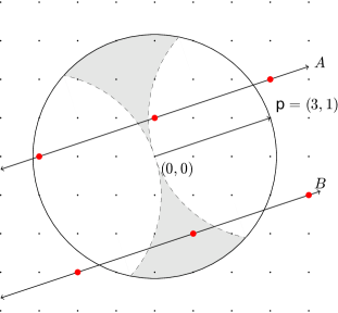
Figure 2.1. The differential equations governing the set of Fourier Coefficients decouple into ‘classes’ when linearised. For $\mathbf{a}\in\mathds{Z}^{2}$, $\dot{\omega}_{\mathbf{a}}$ depends only on $\omega_{\mathbf{a}+\mathbf{p}}$ and $\omega_{\mathbf{a}-\mathbf{p}}$. Extending this idea we get a subset of coefficients that only depend on each other, the class led by $\mathbf{a}$. These coefficients all lie on a straight line with direction $\mathbf{p}$. Classes that do not have an intersection with the disc indicated are stable. Clases that intersect the shaded region indicated at a lattice point have a pair of real eigenvalues (Theorem 3.1). Classes that intersect the disc but do not have intersect the shaded region at a lattice point lead to either a complex quadruplet or two pairs of real eigenvalues.

Figure 2.1 illustrates this idea. Note that the Zeitlin truncated classes $\Sigma^{\prime}_{\mathbf{a}}$ ‘wrap around’ the domain $\mathcal{D}$.

[17] makes the analogous definition for the non-truncated system. In that paper, the classes are infinitely large, and there are infinitely many classes. In our definition, there are finitely many classes of finite size, which depend on the truncation size $N$. As $\mathcal{D}$ is finite, $\Sigma_{\mathbf{a}}$ and $\Sigma^{\prime}_{\mathbf{a}}$ are both finite. Write $\mathbf{p}=(p_{1},p_{2})^{T}$, and $\kappa=\text{gcd}(p_{1},p_{2})$. Then

(2.21) $$\left|\Sigma_{\mathbf{a}}\right|\leq\left\lfloor\frac{2N+1}{\text{max}(p_{1},p_{2})}\right\rfloor$$

and

(2.22) $$\left|\Sigma^{\prime}_{\mathbf{a}}\right|=\frac{2N+1}{\text{gcd}(2N+1,\kappa)}.$$

Note $\left|\Sigma^{\prime}_{\mathbf{a}}\right|$ does not depend on $\mathbf{a}$, and is odd for all choices of $N$ and $\mathbf{p}$. We use this fact many times later. For $\text{gcd}(p_{1},p_{2})=1$, $|\Sigma^{\prime}_{\mathbf{a}}|=2N+1$.

For $\Sigma_{\mathbf{a}}$ we can make a “canonical” choice of $\mathbf{a}$ by selecting $\mathbf{a}$ in a length $|\mathbf{p}|$ strip. For $\Sigma^{\prime}_{\mathbf{a}}$ a canonical choice for $\mathbf{a}$ is found by restricting $\mathbf{a}$ to be in a $|\mathbf{p}|$ by $\frac{|\Sigma^{\prime}_{\mathbf{a}}|}{|\mathbf{p}|}$ rectangle centred around $\mathbf{0}$ oriented so the sides of length $|\mathbf{p}|$ are parallel to $\mathbf{p}$. For the Zeitlin truncation a unique choice is not possible if $\kappa>1$. See Section 4 and 4.1 for details.

Fixing $\mathbf{p}$ and a canonical choice of $\mathbf{a}$ we now restrict our attention to the associated subsystems $\Sigma_{\mathbf{a}}$ and $\Sigma^{\prime}_{\mathbf{a}}$. Introduce new notation

(2.23) $$\omega_{k}=\begin{cases}\omega_{\mathbf{a}+k\mathbf{p}}&\text{ if }\mathbf{a}+k\mathbf{p}{\in}\mathcal{D},\\ 0&\text{ otherwise.}\end{cases}\;\;\;\;\;\;\;\;\;\;\;\;\omega^{\prime}_{k}=\omega_{\widehat{\mathbf{a}+k\mathbf{p}}},$$

(2.24) $$\rho_{k}=\frac{1}{|\mathbf{p}|^{2}}-\frac{1}{|\widehat{\mathbf{a}+k\mathbf{p}}|^{2}}\;\;\text{for}\;\;k=\in\mathbb{Z},$$

(2.25) $$\alpha=\Gamma\mathbf{a}\times\mathbf{p}\in\mathds{R},\;\;\;\alpha^{\prime}=\frac{\Gamma\sin(\varepsilon(\widehat{\mathbf{a}+k\mathbf{p}})\times\mathbf{p})}{\varepsilon}\in\mathds{R}.$$

The value of the coefficient $\rho_{k}$ is related to the distance of the lattice point $\widehat{\mathbf{a}+k\mathbf{p}}$ from the boundary of the disc of radius $|\mathbf{p}|$, where negative values of $\rho_{k}$ correspond to lattice points inside the disc. Note that $\alpha$ does not depend on $k$. Also note that

(2.26) $$\lim_{N\to\infty}\alpha^{\prime}=\lim_{\varepsilon\to 0}\alpha^{\prime}=\Gamma\mathbf{a}\times\mathbf{p}=\alpha.$$

Noting that $\sin(\epsilon(\widehat{\mathbf{k}+\mathbf{p}})\times\mathbf{k})=\sin(\epsilon\mathbf{p}\times\mathbf{k})$ and rewriting (2.17) and (2.18) with the new notation gives a compact form of the linear systems

(2.27) $$\dot{\omega}_{k}=\alpha(\rho_{k+1}\omega_{k+1}-\rho_{k-1}\omega_{k-1}),$$

(2.28) $$\dot{\omega}^{\prime}_{k}=\alpha^{\prime}(\rho_{k+1}\omega^{\prime}_{k+1}-\rho_{k-1}\omega^{\prime}_{k-1}).$$

All indices in (2.28) are written modulo $|\Sigma^{\prime}_{\mathbf{a}}|$.

Let $m_{1},m_{2}\in\mathbb{Z}$ be such that $\mathbf{a}-m_{1}\mathbf{p}\in\mathcal{D}$, $\mathbf{a}-(m_{1}+1)\mathbf{p}\not{\in}\mathcal{D}$ and $\mathbf{a}+m_{2}\mathbf{p}\in\mathcal{D}$, $\mathbf{a}+(m_{2}+1)\mathbf{p}\not{\in}\mathcal{D}$. If we write $\boldsymbol{\omega}=\begin{pmatrix}\omega_{-m_{1}},\;\omega_{-m_{1}+1},\;...,\omega_{-1},\omega_{0},\omega_{+1},\;...,\omega_{m_{2}}\end{pmatrix}^{T}$, then $\boldsymbol{\dot{\omega}}=\alpha A\boldsymbol{\omega}$ where

(2.29) $$A=\begin{pmatrix}0&+\rho_{-m_{1}+1}&0&\cdots&0&0&0\\ -\rho_{-m_{1}}&0&+\rho_{-m_{1}+2}&\cdots&0&0&0\\ 0&-\rho_{-m_{1}+1}&0&\cdots&0&0&0\\ \vdots&\vdots&\vdots&\ddots&\vdots&\vdots&\vdots\\ 0&0&0&\cdots&0&+\rho_{m_{2}-1}&0\\ 0&0&0&\cdots&-\rho_{m_{2}-2}&0&+\rho_{m_{2}}\\ 0&0&0&\cdots&0&-\rho_{m_{2}-1}&0\end{pmatrix}.$$

If we write $\boldsymbol{\omega}^{\prime}=\begin{pmatrix}\omega^{\prime}_{0},\;\omega^{\prime}_{1},\;...,\;\omega^{\prime}_{n-1}\end{pmatrix}^{T}$, then $\boldsymbol{\dot{\omega}}^{\prime}=\alpha^{\prime}A^{\prime}\boldsymbol{\omega}^{\prime}$ where

(2.30) $$A^{\prime}=\begin{pmatrix}0&+\rho_{1}&0&0&\cdots&0&-\rho_{n-1}\\ -\rho_{0}&0&+\rho_{2}&0&\cdots&0&0\\ 0&-\rho_{1}&0&+\rho_{3}&\cdots&0&0\\ 0&0&-\rho_{2}&0&\cdots&0&0\\ \vdots&\vdots&\vdots&\vdots&\ddots&\vdots&\vdots\\ 0&0&0&0&\cdots&0&+\rho_{n-1}\\ +\rho_{0}&0&0&0&\cdots&-\rho_{n-2}&0\end{pmatrix}.$$

If $\mathbf{a}=\mathbf{0}$ or $\mathbf{a}$ is parallel to $\mathbf{p}$, $\alpha=\alpha^{\prime}=0$. Thus the associated class only contributes zero eigenvalues and will not contribute to the linear instability of the system. We can thus ignore the classes with $\alpha=\alpha^{\prime}=0$.

Note that $A$ can be written as $A=JS$ where

(2.31) $$J=\begin{pmatrix}0&+1&0&\cdots&0&0\\ -1&0&+1&\cdots&0&0\\ 0&-1&0&\cdots&0&0\\ \vdots&\vdots&\vdots&\ddots&\vdots&\vdots\\ 0&0&0&\cdots&0&+1\\ 0&0&0&\cdots&-1&0\end{pmatrix},\;\;S=\begin{pmatrix}\rho_{-m_{1}}&0&0&\cdots&0\\ 0&\rho_{-m_{1}+1}&0&\cdots&0\\ 0&0&\rho_{-m_{1}+2}&\cdots&0\\ \vdots&\vdots&\vdots&\ddots&\vdots\\ 0&0&0&\cdots&\rho_{m_{2}}\end{pmatrix}.$$

A similar construction can be made for $A^{\prime}=J^{\prime}S^{\prime}$. As $J$ and $J^{\prime}$ are skew-symmetric and $S$ and $S^{\prime}$ are symmetric, these are (non-canonical) Hamiltonian systems. For both systems, $\mathcal{H}=\sum_{k}\rho_{k}\omega_{k}^{2}$. From this it follows that if $\lambda$ is an eigenvalue of $A$ or $A^{\prime}$ then $-\lambda$, $\bar{\lambda}$ and $-\bar{\lambda}$ are also eigenvalues. Note that $\text{det}(J^{\prime})=0$ as $J^{\prime}$ has odd size, and therefore $J^{\prime}$ is not symplectic with a one-dimensional kernel. $J$ is symplectic if and only if $|\Sigma_{\mathbf{a}}|$ is even.

We now focus on the behaviour of the eigenvalues of $A$ and $A^{\prime}$ as a function of the $\rho_{k}$ values. Note that there is a symmetry in $\mathbf{a}$. For every class $\Sigma_{\mathbf{a}}$ or $\Sigma^{\prime}_{\mathbf{a}}$, the class $\Sigma_{-\mathbf{a}}$ or $\Sigma^{\prime}_{-\mathbf{a}}$ generates the same set of eigenvalues. It is worth noting that $\alpha(-\mathbf{a})=-\alpha(\mathbf{a})$ and $\alpha^{\prime}(-\mathbf{a})=-\alpha^{\prime}(\mathbf{a})$, but as all eigenvalues occur in $\pm$ pairs, this does not affect the spectrum. Thus for the full system rather than a particular class all eigenvalues occur with even multiplicity.

Definition 2.2 (The Unstable Disc).

Introduce the disc $D_{\mathbf{p}}$

(2.32) $$D_{\mathbf{p}}=\{\mathbf{x}\in\mathcal{D}\;|\;|\mathbf{x}|<|\mathbf{p}|\}.$$

This disc is shown in figure 2.1. A simple but important observation is

Lemma 2.3.

A lattice point is inside the unstable disc if and only if the corresponding $\rho$ is negative:

(2.33) $$\widehat{\mathbf{a}+k\mathbf{p}}\in D_{\mathbf{p}}\;\;\iff\;\;\rho_{k}<0.$$

Proof.

This is true as $\rho_{k}<0$ if and only if $|\mathbf{a}+k\mathbf{p}|<|\mathbf{p}|$ from (2.24), which is exactly the condition that $\widehat{\mathbf{a}+k\mathbf{p}}\in D_{\mathbf{p}}$. ∎

This is illustrated in figure 2.1. The point $\mathbf{a}$ inside the disc corresponds to $\rho_{0}<0$ and the other points correspond to $\rho_{k}>0$. Also note that

$$\widehat{\mathbf{a}+k\mathbf{p}}\in\partial D_{\mathbf{p}}\iff\rho_{k}=0.$$

3. Stability and Instability of Classes

3.1. Stable Classes

The matrices $A$ and $A^{\prime}$ are similar to skew-symmetric matrices by conjugation.

(3.1) $$T=\begin{pmatrix}\sqrt{\rho_{-m_{1}}}&0&0&\cdots&0\\ 0&\sqrt{\rho_{-m_{1}+1}}&0&\cdots&0\\ 0&0&\sqrt{\rho_{-m_{1}+2}}&\cdots&0\\ \vdots&\vdots&\vdots&\ddots&\vdots\\ 0&0&0&\cdots&\sqrt{\rho_{m_{2}}}\end{pmatrix},$$

(3.2) $$TAT^{-1}=\begin{pmatrix}0&+\sqrt{\rho_{-m_{1}}\rho_{-m_{1}+1}}&0&\cdots&0\\ -\sqrt{\rho_{-m_{1}}\rho_{-m_{1}+1}}&0&+\sqrt{\rho_{-m_{1}+1}\rho_{-m_{1}+2}}&\cdots&0\\ 0&-\sqrt{\rho_{-m_{1}+1}\rho_{-m_{1}+2}}&0&\cdots&0\\ \vdots&\vdots&\vdots&\ddots&\vdots\\ 0&0&0&\cdots&0\end{pmatrix}.$$

A very similar construction exists for $A^{\prime}$.

If $\rho_{k}>0$ for all $k$, this transformation is real and thus $A$ and $A^{\prime}$ are similar to real skew-symmetric matrices. Thus all eigenvalues are purely imaginary and $A$ and $A^{\prime}$ can be diagonalised and so the class is linearly stable. By (2.33) this condition is true exactly if

(3.3) $$\Sigma_{\mathbf{a}}\cap D_{\mathbf{p}}=\emptyset.$$

This is the finite-dimensional analogue of Li’s Unstable Disc Theorem (Theorem III.1) in [17], though the method of proof used in that paper is naturally very different. A discussion of the details such as choice of $\mathbf{p}$ and $N$ required for (3.3) to hold follows in Section 4. Because of this result, only classes with $\mathbf{a}\in D_{\mathbf{p}}$ can contribute linear instability. Also $\mathbf{a}=\mathbf{0}$ implies $\alpha=\alpha^{\prime}=0$ and so this class cannot contribute linear instability.

3.2. Unstable Classes

For classes with $\mathbf{a}\in D_{\mathbf{p}}$, there are two primary possibilities to consider:

1. There is exactly one intersection between the class and the disc (ie, $\Sigma_{\mathbf{a}}\cap D_{\mathbf{p}}=\{\mathbf{a}\}$). This can only occur when $\mathbf{a}$ is chosen to be in the shaded area indicated in figure 2.1.

2. There are exactly two consecutive intersections between the class and the disc (ie,
   ${\Sigma_{\mathbf{a}}\cap D_{\mathbf{p}}=\{\mathbf{a},\mathbf{a}+\mathbf{p}\}}$ or $\Sigma_{\mathbf{a}}\cap D_{\mathbf{p}}=\{\mathbf{a},\mathbf{a}-\mathbf{p}\}$). This occur when $\mathbf{a}\in D_{\mathbf{p}}$ is chosen outside the shaded area indicated in figure 2.1.

For the Zeitlin style truncation, there is also a third possibility we must consider:

1. There are at least two non-consecutive intersections between the class and the disc (ie, $\mathbf{a}\in\Sigma^{\prime}_{\mathbf{a}}\cap D_{\mathbf{p}}$ and $\widehat{\mathbf{a}+k\mathbf{p}}\in\Sigma_{\mathbf{a}}\cap D_{\mathbf{p}}$ for some $k\neq-1,0,1$).

Note that points on the boundary are treated as being outside the disc. Also note that it is not possible for three consecutive lattice points in a class to be in the unstable disc. If $\mathbf{a}$, $\mathbf{a}-\mathbf{p}$ and $\mathbf{a}+\mathbf{p}$ were are all in $\overline{D_{\mathbf{p}}}$, they would lie along a diameter as $\overline{D_{\mathbf{p}}}$ has diameter $2|\mathbf{p}|$ and the distance from $\mathbf{a}-\mathbf{p}$ to $\mathbf{a}+\mathbf{p}$ is $2|\mathbf{p}|$. Therefore $\mathbf{a}=(0,0)$ and $\mathbf{a}\pm\mathbf{p}\in\partial\overline{D_{\mathbf{p}}}$. This is the only possibility to have three consecutive lattice point in $\overline{D_{\mathbf{p}}}$, and hence $D_{\mathbf{p}}$ can at most contain two consecutive lattice points. Figure 2.1 makes this idea clear.

From our numerical and analytical results we can categorise the spectrum of the class in these three cases:

1. The spectrum has a single pair of real eigenvalues and all other eigenvalues on the imaginary axis. This is proved in Theorem 3.1.

2. The spectrum typically corresponds to a quartet of complex eigenvalues $\pm\alpha\pm\beta i$, and all other eigenvalues on the imaginary axis. It can also correspond to two pairs of real eigenvalues, though seems to be less common.

3. This corresponds to the class ‘wrapping around’ the truncated domain of lattice points and intersecting the disc again; see 4.1. The spectrum is a combination of case (i) and case (ii) according to how successive intersections with the disc occur.

This last case is atypical and does not occur with the Galerkin truncation. Usually this case can be avoided by a proper choice of $N$, however when both entries of $\mathbf{p}$ are even, it cannot be avoided. This is discussed in detail in Section 4, particularly Lemma 4.1.

All our numerical evidence is consistent with the result in [16] that the number of eigenvalues with non-zero real part is $\leq 2|D_{\mathbf{p}}|$ (twice the number of interior lattice points in the unstable disc), and our observation is that this is the exact number of hyperbolic eigenvalues.

For case (i), Theorem 3.1 proves that this case always leads to non-zero real eigenvalues. For some $\mathbf{p}$ and $\mathbf{a}$ leading to case (i), Theorem 3.5 describes an explicit lower bound which is independent of the truncation size $N$ for the real eigenvalues. This agrees with numerically observed results, eg the $\epsilon=0$ inviscid result shown in Figure 2 of [15]. It should be noted that our methods do not preclude the possibility that there are other eigenvalues with non-zero real part unaccounted for; we simply assert that there is at least one eigenvalue with positive real part. This together with the results from [10], [16], and [22] is sufficient to conclude nonlinear instability for the whole system.

For the following section, we consider a general set of parameters $(a_{0},a_{1},...,a_{n-1})$ instead of $\rho_{k}$. Introduce a tridiagonal matrix

(3.4) $$T_{\alpha}^{\beta}=\begin{pmatrix}0&a_{\alpha+1}&0&0&\cdots&0&0\\ -a_{\alpha}&0&a_{\alpha+2}&0&\cdots&0&0\\ 0&-a_{\alpha+1}&0&a_{\alpha+3}&\cdots&0&0\\ 0&0&-a_{\alpha+2}&0&\cdots&0&0\\ 0&0&0&-a_{\alpha+3}&\cdots&0&0\\ \vdots&\vdots&\vdots&\vdots&\ddots&\vdots&\vdots\\ 0&0&0&0&\cdots&0&a_{\beta}\\ 0&0&0&0&\cdots&-a_{\beta-1}&0\end{pmatrix},$$

and its characteristic polynomial

(3.5) $$\mathcal{T}_{\alpha}^{\beta}(x)=\text{det}(xI-T_{\alpha}^{\beta})$$

for some integers $0\leq\alpha<\beta\leq n-1$. Then $\mathcal{T}_{\alpha}^{\beta}(x)$ can be recursively defined by expansion from top left to bottom right

$$\mathcal{T}_{\alpha}^{\alpha}(x)=1,\;\;\;\;\;\;\mathcal{T}_{\alpha}^{\alpha+1}(x)=x^{2}+a_{\alpha+1}a_{\alpha},$$

(3.6) $$\mathcal{T}_{\alpha}^{\beta}(x)=x\mathcal{T}_{\alpha}^{\beta-1}(x)+a_{\beta}a_{\beta-1}\mathcal{T}_{\alpha}^{\beta-2}(x).$$

or by expansion from bottom right to top left

$$\mathcal{T}_{\beta}^{\beta}(x)=1,\;\;\;\;\;\;\mathcal{T}_{\beta-1}^{\beta}(x)=x^{2}+a_{\beta-1}a_{\beta},$$

(3.7) $$\mathcal{T}_{\alpha}^{\beta}(x)=x\mathcal{T}_{\alpha+1}^{\beta}(x)+a_{\alpha}a_{\alpha+1}\mathcal{T}_{\alpha+2}^{\beta}(x).$$

Note that

(3.8) $$a_{k}>0\text{ for all }\alpha\leq k\leq\beta\;\implies\;\mathcal{T}_{\alpha}^{\beta}(x)>0\text{ for all }x>0.$$

This can be seen by the recursive definitions; all terms are positive.

The following is also useful:

(3.9) $$\mathcal{T}_{\alpha}^{\beta}(0)=\begin{cases}\prod_{k=\alpha}^{\beta}a_{k}&\text{if }\beta-\alpha\text{ is odd,}\\ 0&\text{if }\beta-\alpha\text{ is even.}\end{cases}$$

(3.10) $$\left.\frac{\mathrm{d}}{\mathrm{d}x}\mathcal{T}_{\alpha}^{\beta}(x)\right|_{x=0}=\begin{cases}0&\text{if }\beta-\alpha\text{ is odd,}\\ \sum_{k=0}^{\frac{\beta-\alpha}{2}}\left(\prod_{j=\alpha;\;j\neq\alpha+2k}^{\beta}a_{j}\right)&\text{if }\beta-\alpha\text{ is even.}\end{cases}$$

These can be proved by simple induction arguments.

Introduce similar notation for (2.30)

(3.11) $$A^{\prime}=\begin{pmatrix}0&+a_{1}&0&0&\cdots&0&-a_{n-1}\\ -a_{0}&0&+a_{2}&0&\cdots&0&0\\ 0&-a_{1}&0&+a_{3}&\cdots&0&0\\ 0&0&-a_{2}&0&\cdots&0&0\\ \vdots&\vdots&\vdots&\vdots&\ddots&\vdots&\vdots\\ 0&0&0&0&\cdots&0&+a_{n-1}\\ +a_{0}&0&0&0&\cdots&-a_{n-2}&0\end{pmatrix},$$

with the characteristic polynomial

(3.12) $$\mathcal{A}(x)=\text{det}(xI-A).$$

Then, if $n$ is odd,

$$\mathcal{A}(x) =x\mathcal{T}_{0}^{n-2}(x)+a_{n-1}a_{n-2}\mathcal{T}_{0}^{n-3}(x)+a_{n-1}a_{0}\mathcal{T}_{1}^{n-2}(x)$$

(3.13) $$=\mathcal{T}_{0}^{n-1}(x)+a_{0}a_{n-1}\mathcal{T}_{1}^{n-2}(x)$$

This can be demonstrated by expanding by minors along the last row and column of $xI-A$. Recall that $n$ is odd for the relevant problem ($n=|\Sigma_{\mathbf{a}}|$ from equation (2.22)).

We first show that in case (i) there is some non-zero real eigenvalue. Because of the Hamiltonian nature of the system this means there is a plus/minus pair of eigenvalues and so there is linear instability. This is then extended to show that under certain conditions there is pair of real eigenvalues with an explicit lower bound independent of $N$.

Theorem 3.1 (Real Eigenvalues in case (i)).

If $\rho_{0}<0$, and $\rho_{k}\geq 0$ for all $k=1,2,...,n-1$ and $\rho_{k}=0$ for at most one of $k=1,2,...,n-1$, then for sufficiently large $N$, (2.30) has a non-zero real eigenvalue.

Proof.

The characteristic polynomial $\mathcal{A}$ for odd $n$ has leading term $x^{n}$ and constant term $0$. By combining (3.13) and (3.10) (noting that $n$ is odd, so $n-1$ and $n-3$ are even), the linear coefficient is given by

$$\left.\frac{\mathrm{d}\mathcal{A}}{\mathrm{d}x}\right|_{x=0} =\left.\frac{\mathrm{d}}{\mathrm{d}x}\mathcal{T}_{0}^{n-1}(x)\right|_{0}+a_{0}a_{n-1}\left.\mathcal{T}_{1}^{n-2}(x)\right|_{0}$$

$$=\sum_{k=0}^{\frac{n-1}{2}}\left(\prod_{j=0;\;j\neq 2k}^{n-1}a_{j}\right)+\sum_{k=0}^{\frac{n-3}{2}}\left(\prod_{j=1;\;j\neq 1+2k}^{n-2}a_{j}\right)$$

(3.14) $$=\sum_{k=0}^{n-1}\left(\prod_{j=0;\;j\neq k}^{n-1}a_{j}\right)$$

(3.15) $$=\left(\prod_{j=0}^{n-1}a_{j}\right)\left(\sum_{k=0}^{n-1}\frac{1}{a_{k}}\right).$$

Note that (3.15) is only valid for $a_{k}\neq 0$ for all $k$, but (3.14) is always valid . Now let $a_{k}=\rho_{k}$. First assume $\rho_{k}>0$ for all $k\neq 0$. As $\rho_{k}\to\frac{1}{|\mathbf{p}|^{2}}>0$ as $|\widehat{\mathbf{a}+k\mathbf{p}}|\to\infty$ and the size $n$ of the classes grows linearly with $N$, $\sum_{j=0}^{n-1}\frac{1}{a_{j}}=\sum_{j=0}^{n-1}\frac{1}{\rho_{j}}>0$ for sufficiently large $N$ (where $\rho_{k}=a_{k}$). However $\prod_{j=0}^{n-1}a_{j}<0$ as $a_{0}<0$, $a_{j}>0$ for all $j=1,..,n-1$, and hence the linear coefficient of the characteristic polynomial is less than zero.

If $\rho_{k}=0$ for exactly one $k$, then (3.14) consists of only one term, $\prod_{j=0;\;j\neq k}^{n-1}\rho_{j}$. This is less than zero as $\rho_{0}<0$ and $\rho_{j}>0$ for all $j\neq 0,k$.

If $\rho_{k}=0$ for more than one value of $k$, then the linear term is zero and we cannot apply this argument.

As the constant term is zero, and the linear term is non-zero, then the lowest order non-zero coefficient of the polynomial is negative.

We now argue by contradiction. Assume all roots of the polynomial are imaginary (say $i\omega_{k}$) or complex ($\gamma_{j}+i\delta_{j}$) or zero. Then because eigenvalues occur in positive and negative pairs as well as conjugate pairs the polynomial has the form

(3.16) $$\mathcal{A} (x)=$$

$$x^{n_{1}}\prod_{k=1}^{n_{2}}(x-i\omega_{k})(x+i\omega_{k})\prod_{j=1}^{n_{3}}\left[(x-\gamma_{j}-i\delta_{j})(x-\gamma_{j}+i\delta_{j})(x+\gamma_{j}-i\delta_{j})(x+\gamma_{j}+i\delta_{j})\right]$$

(3.17) $$=x^{n_{1}}\prod_{k=1}^{n_{2}}(x^{2}+\omega_{k}^{2})\prod_{j=1}^{n_{3}}\left(x^{4}-2x^{2}(\gamma_{j}^{2}-\delta_{j}^{2})+(\gamma_{j}^{2}+\delta_{j}^{2})^{2}\right).$$

The lowest order non-zero coefficient (of $x^{n_{1}}$) is $\prod_{k=1}^{n_{2}}(\omega_{k}^{2})\prod_{j=1}^{n_{3}}\left((\gamma_{j}^{2}+\delta_{j}^{2})^{2}\right)>0$. Thus by contradiction there must be some real eigenvalue, which will occur in a plus and minus pair.

∎

For the Galerkin case (3.4), although the result is the same we cannot apply the same proof. Since we were not able to show that these eigenvalues remain bounded away from the imaginary axis when $N\to\infty$ we now show in a different way that for both truncations there are eigenvalues whose real part is bounded away from zero for $N\to\infty$. These proofs have stricter conditions on the $\rho_{k}$ then Theorem 3.1, but we will see that they can be met for most $\mathbf{p}$.

Lemma 3.2 (Lower Bound for Real Eigenvalue (Zeitlin)).

If $a_{0}<0$, and $a_{k}>0$ for all $k\neq 0$, and $a_{0}+a_{2}<0$, then

(3.18) $$\mathcal{A}(\sqrt{-a_{1}(a_{0}+a_{2})})<0.$$

Proof.

By expanding (3.13) using (3.7),

(3.19) $$\mathcal{A}(x)= (x^{3}+(a_{0}a_{1}+a_{1}a_{2})x)\mathcal{T}_{3}^{n-1}(x)$$

$$+(x^{2}+a_{0}a_{1})a_{2}a_{3}\mathcal{T}_{4}^{n-1}(x)$$

$$+a_{0}a_{n-1}\mathcal{T}_{1}^{n-2}(x).$$

Thus

(3.20) $$\mathcal{A}(\sqrt{-a_{1}(a_{0}+a_{2})})= -a_{1}a_{2}^{2}a_{3}\mathcal{T}_{4}^{n-1}(\sqrt{-a_{1}(a_{0}+a_{2})})\$$

$$+a_{0}a_{n-1}\mathcal{T}_{1}^{n-2}(\sqrt{-a_{2}(a_{1}+a_{3})}).$$

As $a_{1},a_{2},a_{3},a_{n-1}>0$, $a_{0}<0$ and the $\mathcal{T}$ terms are positive by (3.8) the result follows. ∎

We make a similar case for the Galerkin truncation

Lemma 3.3 (Lower Bound for Real Eigenvalue (Galerkin)).

If $\beta>0$, $a_{0}<0$, and $a_{k}>0$ for all $k\neq 0$, and $a_{0}+a_{2}<0$, then

(3.21) $$\mathcal{T}_{\alpha}^{\beta}(\sqrt{-a_{1}(a_{0}+a_{2})})<0.$$

Proof.

Begin by noting that

(3.22) $$\mathcal{T}_{\alpha}^{\gamma}(\sqrt{-a_{1}(a_{0}+a_{2})})\geq 0$$

for all $\gamma<0$ by (3.8). By expanding (3.7),

(3.23) $$\mathcal{T}_{\alpha}^{1}(x) =(x^{2}+a_{1}a_{0})\mathcal{T}_{\alpha}^{-1}(x)+a_{0}a_{-1}x\mathcal{T}_{\alpha}^{-2}(x)$$

(3.24) $$\mathcal{T}_{\alpha}^{1}(\sqrt{-a_{1}(a_{0}+a_{2})}) =-a_{1}a_{2}\mathcal{T}_{\alpha}^{-1}(\sqrt{-a_{1}(a_{0}+a_{2})})$$

$$+a_{0}a_{-1}\sqrt{-a_{1}(a_{0}+a_{2})}\mathcal{T}_{\alpha}^{-2}(\sqrt{-a_{1}(a_{0}+a_{2})}).$$

As $a_{0}<0$, $a_{k}>0$ for all $k\neq 0$, and $\mathcal{T}_{\alpha}^{-1},\mathcal{T}_{\alpha}^{-2}$ take positive values for positive arguments, $\mathcal{T}_{\alpha}^{1}(\sqrt{-a_{1}(a_{0}+a_{2})})<0$.

Now similar to the proof of 3.2,

(3.25) $$\mathcal{T}_{\alpha}^{2}(\sqrt{-a_{1}(a_{0}+a_{2})})= (x^{2}+a_{1}(a_{0}+a_{2}))x\mathcal{T}_{\alpha}^{-1}(\sqrt{-a_{1}(a_{0}+a_{2})})$$

$$+(x^{2}+a_{2}a_{1})a_{0}a_{-1}\mathcal{T}_{\alpha}^{-2}(\sqrt{-a_{1}(a_{0}+a_{2})})$$

$$=-a_{1}a_{0}^{2}a_{-1}\mathcal{T}_{\alpha}^{-2}(\sqrt{-a_{1}(a_{0}+a_{2})}).$$

As $a_{1},a_{-1}>0$, $a_{0}<0$ and the $\mathcal{T}$ terms are positive by (3.8) it follows that

$$\mathcal{T}_{\alpha}^{2}(\sqrt{-a_{1}(a_{0}+a_{2})})<0.$$

Now if $\gamma>2$, we can make a recursive argument:

(3.26) $$\mathcal{T}_{\alpha}^{\gamma}(x)=x\mathcal{T}_{\alpha}^{\gamma-1}(x)+a_{\gamma}a_{\gamma-1}\mathcal{T}_{\alpha}^{\gamma-2}(x).$$

Now $x=\sqrt{-a_{1}(a_{0}+a_{2})}>0$ and $a_{\gamma}a_{\gamma-1}>0$ (as $\gamma>2$). By inductive reasoning, as $\mathcal{T}_{\alpha}^{1}<0,$ $\mathcal{T}_{\alpha}^{2}<0$, then $\mathcal{T}_{\alpha}^{\gamma}<0$ for all $\gamma>2$. Therefore $T_{\alpha}^{\beta}(\sqrt{-a_{1}(a_{0}+a_{2})})<0$. ∎

We can also make a similar construction if $a_{0}<0$, $a_{k}\geq 0$ for all $k\neq 0$ and $a_{0}+a_{n-2}<0$. In this case, $\mathcal{A}(\sqrt{-a_{n-1}(a_{0}+a_{n-2})})\leq 0$.

Lemma 3.4.

Assuming the same conditions as Lemma 3.2 and Lemma 3.3, there exists some

$$x_{1}^{*},x_{2}^{*}>\sqrt{-a_{1}(a_{0}+a_{2})}$$

such that $\mathcal{T}_{\alpha}^{\beta}(x_{1}^{*})=0$, $\mathcal{A}(x_{2}^{*})=0$.

Proof.

The leading order term of $\mathcal{A}(x)$ is always $x^{n}$ regardless of $a_{0},...,a_{n-1}$, and $\mathcal{A}(x)$ is real for real $x$. Thus $\lim_{x\to\infty}\mathcal{A}(x)>0$. But by Lemma 3.2 $\mathcal{A}(\sqrt{-a_{1}(a_{0}+a_{2})})<0$, and the result follows by the intermediate value theorem.

The same argument can be applied to $\mathcal{T}_{\alpha}^{\beta}(x)$, with the equivalent result. ∎

We now turn our attention back to the context of our problem.

Theorem 3.5 (Lower Bound for Real Eigenvalues in case (i)).

If $\mathbf{a}\in D_{\mathbf{p}}$ and ${\mathbf{a}+k\mathbf{p}}\not{\in}\bar{D}_{\mathbf{p}}$ (equivalently $\widehat{\mathbf{a}+k\mathbf{p}}\not{\in}\bar{D}_{\mathbf{p}}$) for $k=1,2,..,n-1$ and

(3.27) $$\lambda^{\dagger}=\sqrt{-\rho_{1}(\rho_{0}+\rho_{2})}$$

is real, there exist $\lambda_{1},\lambda_{2}>\lambda^{\dagger}$ such that $\lambda_{1}$ is an eigenvalue of (2.29) and $\lambda_{2}$ is an eigenvalue of (2.30).

Similarly if $\lambda^{\dagger}=\sqrt{-\rho_{n-1}(\rho_{0}+\rho_{n-2})}$ is real there exist $\lambda_{1},\lambda_{2}>\lambda^{\dagger}$ such that $\lambda_{1}$ is an eigenvalue of (2.29) and $\lambda_{2}$ is an eigenvalue of (2.30).

Proof.

This follows from the previous three lemmas, letting $\rho_{i}=a_{i}$ and making note of (2.33). ∎

Section 4 clarifies under what conditions $\lambda^{\dagger}$ is real, and Theorem 3.5 holds. For example, when $\mathbf{p}=(1,1)^{T}$ then $\mathbf{a}=(0,1)^{T}$ leads to a case (i) class, so Theorem 3.1 holds, but the reality conditions in Theorem 3.5 are not satisfied. It is also possible that $\lambda^{\dagger}=0$, so the real eigenvalue could be zero, so we also require that $\lambda^{\dagger}>0$. A sufficient condition on $\mathbf{a}$ for this to hold is given in Lemma 4.2.

3.3. Associated Eigenvector

We must also consider whether this eigenvalue is “valid” in the sense that the corresponding eigenfunction in the full system is in fact a function in $L^{2}(\mathbb{T}^{2})$, the square integrable function on the torus. For this we need to show that the Fourier coefficients are in $\ell^{2}$. In this section we are going to work with the infinite dimensional system. The reason for this is that although the truncations are useful in the calculation of eigenvalues, it is simpler to analyse the corresponding eigenvectors in the full system. Thus our approach is to use the finite dimensional Zeitlin truncation to compute the eigenvalues, then take the limit as $N\to\infty$, and then study the decay of the corresponding eigenvector.

Consider the linearised matrix for the full system

(3.28) $$M=\begin{pmatrix}\ddots&\vdots&\vdots&\vdots&\vdots&\ddots\\ \cdots&0&\rho_{0}&0&0&\cdots\\ \cdots&-\rho_{-1}&0&\rho_{1}&0&\cdots\\ \cdots&0&-\rho_{0}&0&\rho_{2}&\cdots\\ \cdots&0&0&-\rho_{1}&0&\cdots\\ \ddots&\vdots&\vdots&\vdots&\vdots&\ddots\end{pmatrix}.$$

This is the limit in some sense of the matrices (2.29) and (2.30) which corresponds to the limit of the Hamiltonian systems $A=JS$ and $A^{\prime}=J^{\prime}S^{\prime}$ with Hamiltonian $\mathcal{H}(\mathbf{\omega})=\sum_{k}\rho_{k}\omega_{k}^{2}$.

Lemma 3.6.

The infinite dimensional linearised system given by (3.28) has a positive real eigenvalue $\lambda$ under the same conditions as Theorem 3.5. Furthermore, the associated eigenvector is in $\ell^{2}$.

Proof.

According to Theorem 3.5, there exist positive real eigenvalues with some lower bound (independent of $N$) of (2.30) (and (2.29)) for any $N$ and either choice of truncation. By taking $N\to\infty$ we can conclude there exists some positive real eigenvalue $\lambda$ of (3.28).

Now consider an eigenvector associated with this eigenvalue, $\mathbf{v}=(...,v_{-1},v_{0},v_{1},v_{2},...)^{T}$. For this to correspond to a real $L^{2}$ eigenfunction of the full problem (that is, for the Fourier series to converge), we need these Fourier coefficients to decay sufficiently fast: they need to be a sequence in $\ell^{2}$.

The entries of the (infinite dimensional) eigenvector $v_{k}$ of (3.28) corresponding to eigenvalues $\lambda$ satisfy the recursion relation

(3.29) $$\lambda v_{k}=\rho_{k+1}v_{k+1}-\rho_{k-1}v_{k-1}.$$

Since all $\rho_{k}\not=0$ this can be rewritten as

(3.30) $$v_{k+1}=\frac{\lambda}{\rho_{k+1}}v_{k}+\frac{\rho_{k-1}}{\rho_{k+1}}v_{k-1}.$$

Consider the limiting behaviour as $k\to\infty$. then $\rho_{k}\to\frac{1}{|\mathbf{p}|^{2}}$. In this limit solutions to (3.30) behave like solutions to

(3.31) $$v_{k+1}={\lambda}|\mathbf{p}|^{2}v_{k}+v_{k-1},$$

see, e.g., [11].

This linear recurrence has the general solution

(3.32) $$v_{k}=C_{1}\mu_{1}^{k}+C_{2}\mu_{2}^{k}$$

where $C_{1},C_{2}\in\mathbb{R}$ are constants and $\mu_{1},\mu_{2}$ are solutions to $\mu^{2}-\lambda|\mathbf{p}|^{2}\mu-1=0$. Thus $\mu_{1}\mu_{2}=-1$ and without loss of generality $|\mu_{1}|<1$, $|\mu_{2}|>1$ (note that we cannot have $|\mu_{1}|=|\mu_{2}|=1$ as $\lambda|\mathbf{p}|^{2}\neq 0$).

Now as $\mathbf{v}$ is an eigenvector associated with a real eigenvalue, the span of the eigenvector is an invariant subspace of the Hamiltonian system with Hamiltonian $\mathcal{H}(\mathbf{\omega})=\sum_{k}\rho_{k}\omega_{k}^{2}$. In fact, let $\mathbf{\omega}(0)=\mathbf{v}$, then $\mathbf{\omega}(t)=e^{\lambda t}\mathbf{v}$. As the Hamiltonian is an integral of the motion, $\mathcal{H}(\mathbf{v})=\mathcal{H}(e^{\lambda t}\mathbf{v})$. By taking the limit $t\to-\infty$, $\mathcal{H}(\mathbf{v})=\mathcal{H}(0)=0$.

Therefore,

(3.33) $$\mathcal{H}(\mathbf{v})=\sum_{k}\rho_{k}v_{k}^{2}=0;$$

(3.34) $$\sum_{k\neq 0}\rho_{k}v_{k}^{2}=-\rho_{0}v_{0}^{2}.$$

Now, if $C_{2}\neq 0$,

(3.35) $$\sum_{k\neq 0}\rho_{k}v_{k}^{2}\sim\sum_{k\neq 0}\rho_{k}(C_{2}\mu_{2}^{k})^{2}\to\infty,$$

recalling that $\rho_{k}\to\frac{1}{|\mathbf{p}|^{2}}$ and $\rho_{k}>0$ for all $k\neq 0$. But $|\rho_{0}|<1$ and $v_{k}$ is finite, so there is a contradiction. Thus $C_{2}=0$ and $v_{k}=C_{1}\mu_{1}^{k}$ in the asymptotic limit, where $|\mu_{1}|<1$. This is exponential decay, which is sufficient for the Fourier series to converge.

Similarly for $k\to-\infty$, the limiting behaviour is governed by

(3.36) $$v_{k-1}=-{\lambda}|\mathbf{p}|^{2}v_{k}+v_{k-1}.$$

Again, this means $v_{k}$ is asymptotic to $C_{1}\mu_{1}^{k}+C_{2}\mu_{2}^{k}$ for $|\mu_{1}|<1$, $|\mu_{2}|>1$. By the same argument as above, we can conclude that $C_{1}=0$ and so $v_{k}=C_{2}\mu_{2}^{k}$ as $k\to\infty$. Thus the Fourier coefficients decay exponentially on both sides with $|k|$, and hence $\mathbf{v}$ is in $\ell^{2}$. ∎

4. Instability of Equilibria

Figure 4.1. For fixed $\mathbf{p}$ and $\mathbf{a}$, there are some concerns with the wrapping of the Zeitlin truncation and the way this affects the intersection $\Sigma_{\mathbf{a}}\cap D_{\mathbf{p}}$. These situations are discussed in Lemma 4.1.
                                                                                                                                                  Left: the shortest distance between $\mathbf{a}$ and some non-consecutive $\widehat{\mathbf{a}+k\mathbf{p}}$ is at least $\frac{2N+1}{|\mathbf{p}|}$. As we are interested in the limit $N\to\infty$, this distance can be made arbitrarily large, so that $\frac{2N+1}{|\mathbf{p}|}>2|\mathbf{p}|$. This ensures that $\mathbf{a}$ and $\widehat{\mathbf{a}+k\mathbf{p}}$ cannot both be in the disc $D_{\mathbf{p}}$.
                                                                                                                                                  Right: The situation where there exists $k\in\mathds{R}$ such that $\widehat{\mathbf{a}+k\mathbf{p}}$ lies on the line segment between $\mathbf{a}$ and $\mathbf{a}+\mathbf{p}$. This causes problems for our values of $\rho$. For $\widehat{\mathbf{a}+k\mathbf{p}}$ to lie at a lattice point on the line segment, $\text{gcd}(p_{1},p_{2})>1$. If $\text{gcd}(p_{1},p_{2})$ is odd, we can avoid this situation by choosing $N$ per Equation (4.1); if $p_{1}$ and $p_{2}$ are both even this situation is unavoidable.

To prove instability of an equilibrium for a given $\mathbf{p}$ we need to find at least one unstable class $\Sigma_{\mathbf{a}}/\Sigma^{\prime}_{\mathbf{a}}$. A necessary condition for a lattice point $\mathbf{a}$ to lead to an unstable class is to be inside the unstable disc. More precisely we desire a lattice point $\mathbf{a}$ that leads to a class of case (i) as this is the simplest situation for us to deal with. Theorem 3.5 asserts that there is a real eigenvalue with an explicit lower bound under some certain conditions. The goal now is to determine for which $\mathbf{p}$ there exists a lattice point $\mathbf{a}$ such that the conditions of Theorem 3.5 are satisfied.

There are a number of other considerations when we take Zeitlin’s truncation. Although this preserves the geometric structure and the Casimirs of the original problem, it introduces a problem that is not present in [17]. This has already been mentioned in the classification of classes; it is the appearance of case (iii), in which a class intersects the unstable disc at non-consecutive points. This may occur because now we have periodic boundary conditions not only in physical space, but also in Fourier space. There are two distinct problems caused by this, as illustrated in figure 4.1.

The lattice points of a class lie on parallel line segments with direction vector $\mathbf{p}$ in the domain of Fourier modes. In the Zeitlin truncation there is more than one such line segment in the domain. The first problem appears when the distance between these line segments is so small that more than one line segment intersects the unstable disc. This can be fixed by making $N$ sufficiently large. The second problem occurs when non-consecutive lattice points lie on the same line segment intersecting the unstable disc. If $\text{gcd}(p_{1},p_{2})$ is not even this can be fixed by choosing $N$ per (4.1). Note that for our purposes, $\mathrm{gcd}(p_{1},0)=p_{1}$ and $\mathrm{gcd}(p_{1},p_{2})=\mathrm{gcd}(|p_{1}|,|p_{2}|)$.

Lemma 4.1 (Correct choices of $N$ for the Zeitlin truncation).

For all $\mathbf{p}=(p_{1},p_{2})^{T}$ such that $\kappa=\mathrm{gcd}(p_{1},p_{2})$ is not even, there exists a sequence of $N$ which increases without bound such that for all choices of $\mathbf{a}$ any two non-consecutive lattice points in $\Sigma^{\prime}_{\mathbf{a}}$ cannot both be in the unstable disc.

Proof.

Let

(4.1) $$N=\frac{(2\tilde{N}+1)\kappa-1}{2}$$

for $A\in\mathds{N}$. Thus $2N+1=(2\tilde{N}+1)\kappa$. If $\kappa$ is not even, then such an $N$ is a positive integer and thus a valid grid size. Select as a lower bound $\tilde{N}>\frac{2|\mathbf{p}|^{2}-\kappa}{2\kappa}$ so that $N>\frac{2|\mathbf{p}|^{2}-1}{2}$. $\mathbf{p}$ is fixed and finite so this lower bound is always finite. We can thus find an infinite sequence of $N$ that increases without bound by letting $\tilde{N}$ increase without bound.

If $\mathbf{x}\in\Sigma_{\mathbf{a}}$ then $\mathbf{x}=\widehat{\mathbf{a}+k\mathbf{p}}$ for some $k\in\mathds{N}$. Thus $\mathbf{x}$ lies on the line parallel to the vector $\mathbf{p}$ that passes through the point $\mathbf{a}+\mathbf{\Delta}_{\mathbf{x}}(2N+1)$ for some $\mathbf{\Delta}_{\mathbf{x}}\in\mathds{Z}^{2}$ (note that this point will be outside the domain $\mathcal{D}$).

Similarly if $\mathbf{y}\in\Sigma_{\mathbf{a}}$ then it lies on the line parallel to $\mathbf{p}$ that passes through $\mathbf{a}+\mathbf{\Delta}_{\mathbf{y}}(2N+1)$ for some $\mathbf{\Delta}_{\mathbf{y}}\in\mathds{Z}^{2}$. Then the distance between these two lines is

(4.2) $$d=\frac{|((\mathbf{a}+\mathbf{\Delta}_{\mathbf{x}}(2N+1))-(\mathbf{a}+\mathbf{\Delta}_{\mathbf{y}}(2N+1)))\times\mathbf{p}|}{|\mathbf{p}|}=\frac{(2N+1)|(\mathbf{\Delta}_{\mathbf{x}}-\mathbf{\Delta}_{\mathbf{y}})\times\mathbf{p}|}{|\mathbf{p}|}.$$

$(\mathbf{\Delta}_{\mathbf{x}}-\mathbf{\Delta}_{\mathbf{y}})\times\mathbf{p}\in\mathds{Z}^{2}$, so $d=0$ or $d\geq\frac{2N+1}{|\mathbf{p}|}$. If $d\geq\frac{2N+1}{|\mathbf{p}|}$, this corresponds to $\mathbf{x}$ and $\mathbf{y}$ lying on different line segments, as in figure 4.1. Thus the distance between two points on different line segments is at least $\frac{2N+1}{|\mathbf{p}|}>2|\mathbf{p}|$ for our choice of $N$.

If $d=0$, then $\mathbf{x}$ and $\mathbf{y}$ must lie on the same line segment. Thus $\mathbf{y}$ lies on the line parallel to $\mathbf{p}$ passing through $\mathbf{x}$.

Write $\mathbf{p}=\kappa\mathbf{q}$ so $\mathbf{q}=(q_{1},q_{2})^{T}$ where $\text{gcd}(q_{1},q_{2})=1$. Then as $\mathbf{x},\mathbf{y}\in\mathds{Z}^{2}$, $\mathbf{y}=\mathbf{x}+k\mathbf{q}$ for some $k\in\mathds{Z}$. But $\mathbf{x},\mathbf{y}\in\Sigma_{\mathbf{a}}$ so $\mathbf{y}=\mathbf{x}+j\mathbf{p}+(2N+1)\mathbf{\Delta}$ for some $\mathbf{\Delta}\in\mathds{Z}^{2}$.

Thus $k\mathbf{q}=j\mathbf{p}+(2N+1)\mathbf{\Delta}$. So

(4.3) $$k\mathbf{q}=j\kappa\mathbf{q}+(2\tilde{N}+1)\kappa\mathbf{\Delta}=\kappa(j\mathbf{q}+(2\tilde{N}+1)\mathbf{\Delta}).$$

Thus $k\mathbf{q}$ is divisible by $\kappa$, but the elements of $\mathbf{q}$ both be divided by $\kappa$ by definition, so $\kappa|k$. Thus $\mathbf{y}=\mathbf{x}+\kappa\beta\mathbf{q}$ for some $\beta\in\mathds{Z}$, and so $\mathbf{y}=\mathbf{x}+\beta\mathbf{p}$. Then if $|\mathbf{y}-\mathbf{x}|<2|\mathbf{p}|$ (the necessary condition for $\mathbf{x},\mathbf{y}$ both in $D_{\mathbf{p}}$) this implies $\beta=0$ or $\beta=\pm 1$, and the result follows. ∎

Figure 4.2. If $\mathbf{a}$ is inside the dashed blue circle centred at the origin, then $\rho_{0}+\rho_{2}<0$ and $\rho_{0}+\rho_{n-2}<0$. This circle has centre $(0,0)$ and radius $(\sqrt{3}-1)|\mathbf{p}|$. The shaded region here shows the overlap of this condition and the shaded region in figure 2.1. To show that there is at least one lattice point in the shaded regions we show the disc $D_{c}$ inscribed in this region (indicated by the small shaded red circles) has radius larger than $\nicefrac{{1}}{{\sqrt{2}}}$.

The outstanding issue with Zeitlin’s truncation is that there is no appropriate choice of $N$ when $\gcd(p_{1},p_{2})$ is even. If $\kappa>1$ and $\gcd(\kappa,2N+1)=1$, then $\mathbf{p}$ will generate all multiples of $\mathbf{q}$ due to the wrapping operation. Thus classes that intersect the disc can return after leaving the disc and intersect the disc again, breaking the assumption of 3.2 that $\rho_{k}<0$ for only one value of $k$. This behaviour continues for all values of $N$ with $\gcd(\kappa,2N+1)=1$. If $\kappa$ is even, this is true for any $N$; if $\kappa$ is odd, we select appropriate $N$ to avoid this.

It is important to note that this is not an error per se, but merely a failure of Lemma 4.1 for our proof. The wrapping of the Zeitlin truncation associates modes in an artificial way, but still generates correct results. For instance if $\mathbf{p}=(6,2)^{T}=2(3,1)^{T}$, the class led by $\mathbf{a}=(1,6)^{T}$ intersects the unstable disc again at $(-2,5)^{T}=(1,6)^{T}-(3,1)^{T}$ for any finite truncation size. If we compare the non-imaginary eigenvalues of the class led by $\mathbf{a}=(1,6)^{T}$ with those of the Galerkin-truncated systems for $\mathbf{a}=(1,6)^{T}$ and $\mathbf{a}=(-2,5)^{T}$, the same eigenvalues are generated, with similar convergence to Figure 5.2.

Fortunately, this problem does not arise with the Galerkin truncation as the wrapping operation is omitted, and so the proof goes through without issue. For both truncations it is still necessary to establish whether for a given $\mathbf{p}$ there is an $\mathbf{a}$ such that the conditions of Theorem 3.5 are met. We address that now.

Lemma 4.2.

For all $\mathbf{p}=(p_{1},p_{2})^{T}$ except $(1,0)^{T},(1,1)^{T},(1,2)^{T}$ (and permutations and sign changes thereof) there exists a choice of $\mathbf{a}$ such that the reality conditions of Theorem 3.5 are satisfied for an appropriate choice of $N$ in the Galerkin truncation. Furthermore, if $\kappa=\mathrm{gcd}(p_{1},p_{2})$ is not even there is also a choice of $\mathbf{a}$ such that the conditions of Theorem 3.5 are satisfied for the Zeitlin truncation.

Proof.

For the bounds given in Theorems 3.3 and 3.2 to be real, positive, and hence a valid bound, we require $\rho_{0}<0$, $\rho_{k}\geq 0$ for all $k\neq 0$, and $\rho_{0}+\rho_{2}<0$ (or $\rho_{0}+\rho_{n-2}<0$).

If $\rho_{0}<0,\;\rho_{1},\rho_{-1}>0$, then $|\mathbf{a}|<|\mathbf{p}|$ and $|\mathbf{a}\pm\mathbf{p}|>|\mathbf{p}|$. This is true if and only if $\mathbf{a}$ is in the shaded region figure 2.1. In the Galerkin truncation, this is sufficient to show that $\rho_{k}>0$ for all $k\neq 0$. By Lemma 4.1, in the Zeitlin truncation we can find an unbounded sequence of choices of $N$ such that this is sufficient to show $k\neq 0,\;\;\rho_{k}>0$. Thus for an appropriate choice of $N$ we only need to prove that there exists an $\mathbf{a}$ such that $|\mathbf{a}\pm\mathbf{p}|>|\mathbf{p}|$.

As $\lambda^{\dagger}=\sqrt{-\rho_{1}(\rho_{0}+\rho_{2})}$ (or equivalently $\lambda^{\dagger}=\sqrt{-\rho_{-1}(\rho_{0}+\rho_{-2})}$) is required to be real and non-zero, and $\rho_{-1}>0$, then $\rho_{0}+\rho_{2}<0$ (equivalently $\rho_{0}+\rho_{-2}<0$).

If $|\mathbf{a}|<(\sqrt{3}-1)|\mathbf{p}|$, then $|\mathbf{a}\pm 2\mathbf{p}|\leq|\mathbf{a}|+2|\mathbf{p}|<(\sqrt{3}+1)|\mathbf{p}|$. So

(4.4) $$\rho_{0}+\rho_{\pm 2} <\frac{2}{|\mathbf{p}|^{2}}-\frac{1}{|(\sqrt{3}-1)\mathbf{p}|^{2}}-\frac{1}{|(\sqrt{3}+1)\mathbf{p}|^{2}}$$

$$=0.$$

We thus need to show there exists some lattice point $\mathbf{a}$ such that $|\mathbf{a}|<(\sqrt{3}-1)|\mathbf{p}|$ and $|\mathbf{a}\pm\mathbf{p}|>|\mathbf{p}|$. These two conditions are illustrated in figure 4.2 in the shaded region. Note that this is sufficient but not necessary for Theorem 3.5 to hold.

The idea now is to specify that $\mathbf{a}$ is in the disc inscribed by the shaded region in figure 4.2, which we call $D_{c}$. This disc is tangent to the circles with radii $|\mathbf{p}|$ and centres $\pm\mathbf{p}$ and the circle centred at the origin with radius $(\sqrt{3}-1)|\mathbf{p}|$. It is a simple geometric exercise to show that such a circle has centre $\pm\frac{1}{\sqrt{3}}\begin{pmatrix}-p_{2}\\ p_{1}\end{pmatrix}$ and radius $\left(\frac{2}{\sqrt{3}}-1\right)|\mathbf{p}|$.

If $\mathbf{a}\in D_{c}$, it is outside the circle with centre $-\mathbf{p}$ and radius $|\mathbf{p}|$. Thus $\mathbf{a}+\mathbf{p}$ is outside $D_{\mathbf{p}}$ and $\rho_{1}>0$. Similarly, $\rho_{-1}>0$. As $D_{c}$ is inside the disc with centre origin and radius $\left(\frac{2}{\sqrt{3}}-1\right)|\mathbf{p}|$ clearly $\rho_{0}<0$ and by the above $\rho_{0}+\rho_{\pm 2}<0$. If we take a Zeitlin truncation, choose appropriate $N$ such that $\rho_{k}\geq 0$ for all $k\neq 0$ by Lemma 4. Then the conditions of Theorem 3.5 are satisfied and the resulting bound $\lambda^{\dagger}$ is real and positive.

All that remains is to show that there exists an integer lattice point $\mathbf{a}\in D_{c}$. Any disc with a radius greater than $\frac{1}{\sqrt{2}}$ must contain some integer lattice point (as it wholly contains a square of side length $1$). Thus if

(4.5) $$|\mathbf{p}|>\frac{\sqrt{3}}{\sqrt{2}(2-\sqrt{3})}\approx 4.57.$$

then the $D_{c}$ has radius greater than $\sqrt{2}$ and such a lattice point exists. Note that this is a sufficient but not necessary condition on $\mathbf{p}$ .

Checking the small number of $\mathbf{p}$ values with $|\mathbf{p}|<4.57$ and $\kappa$ odd there are appropriate lattice points $\mathbf{a}$ for most such $\mathbf{p}$. The following table shows an appropriate value for $\mathbf{a}$ for most such $\mathbf{p}$, and “None” where no such $\mathbf{a}$ exists.

(4.6) $$\begin{array}[]{|c | c | c | c | c | c | c | }\hline\cr\mathbf{p}&(4,1)^{T}&(3,3)^{T}&(3,2)^{T}&(3,1)^{T}&(3,0)^{T}&(2,2)^{T}\\ \hline\cr\mathbf{a}&(1,-2)^{T}&(1,-1)^{T}&(1,-2)^{T}&(1,-2)^{T}&(0,2)^{T}&(-1,2)^{T}\\ \hline\cr\end{array}$$

For reflections/rotations of these values of $\mathbf{p}$ the corresponding reflection/rotation of $\mathbf{a}$ is an appropriate choice.

Thus for all $\mathbf{p}=(p_{1},p_{2})^{T}$ such that $\kappa=\mathrm{gcd}(p_{1},p_{2})$ except except $(1,0)^{T},(1,1)^{T},(1,2)^{T}$ and reflections and rotations of these, there is a choice of $\mathbf{a}$ so that the conditions of Theorem 3.5 is satisfied when ${N=\frac{(2\tilde{N}+1)\kappa-1}{2}}$ for any $\tilde{N}>\frac{2|\mathbf{p}|^{2}-\kappa}{2\kappa}$. ∎

Now we can combine the results about eigenvalues and eigenvectors from the last section and the conditions on $\mathbf{p}$ when they are applicable in our main

Theorem 4.3.

The steady state $\Omega^{*}=\alpha\cos(\mathbf{p}\cdot\mathbf{x})+\beta\sin(\mathbf{p}\cdot\mathbf{x})$ is nonlinearly unstable for all $\mathbf{p}=(p_{1},p_{2})^{T}$ except $\mathbf{p}=\begin{pmatrix}\pm 1,0\end{pmatrix}^{T}$, $\mathbf{p}=\begin{pmatrix}0,\pm 1\end{pmatrix}^{T}$ and possibly $\mathbf{p}=\begin{pmatrix}\pm 1,\pm 1\end{pmatrix}^{T}$, $\mathbf{p}=\begin{pmatrix}\pm 2,\pm 1\end{pmatrix}^{T}$, $\mathbf{p}=\begin{pmatrix}\pm 1,\pm 2\end{pmatrix}^{T}$.

Proof.

By Lemma 4.2, for all $\mathbf{p}$ except those listed above there exists some $\mathbf{a}$ such that $\rho_{0}<0$ and $\rho_{0}+\rho_{2}<0$ (or $\rho_{0}+\rho_{n-2}<0$) for an appropriate choice of $N$. Thus by Theorem 3.5 there exists a real positive eigenvalue $\lambda$. Moreover, the eigenvalue is greater than $\sqrt{-\rho_{1}(\rho_{0}+\rho_{2})}$ (or $\sqrt{-\rho_{n-1}(\rho_{0}+\rho_{n-2})}$) which is both positive and independent of the choice of truncation size $N$. The truncation size $N$ can be increased without bound, by Lemma 4.1. Hence there is a hyperbolic eigenvalue in the limit $N\to\infty$ and the spectrum of the PDE is unstable. Now recall that any steady state $\Omega^{*}=\alpha\cos(\mathbf{p}\cdot\mathbf{x})+2\beta\sin(\mathbf{p}\cdot\mathbf{x})$ can be rewritten as $\Omega^{*}=2\Gamma\cos(\mathbf{p}\cdot\tilde{\mathbf{x}})$ and so the full result follows.

By Lemma 3.6, the eigenvector associated with the eigenvalue $\lambda$ is in $\ell^{2}$. The classes led by $\mathbf{a}$ and $-\mathbf{a}$ have the same eigenvalue, and the the corresponding eigenvectors can be combined to construct coefficients $\omega_{\mathbf{k}}$ of a real eigenfunction $\Omega_{\lambda}$ corresponding to $\lambda$. Since the eigenvectors $\mathbf{v}$ are in $\ell^{2}$ the periodic function $\Omega_{\lambda}$ is in $L^{2}$. Together with the result in [16], which shows that the spectral mapping theorem holds, establishes linear instability. To conclude nonlinear instability we refer to the work of [10] and [22]. In [10] it was shown that sufficient conditions for nonlinear instability are linear instability together with a ‘spectral gap’ condition. In [22] it was shown that the essential spectrum of the linearised Euler operator in the cases we are considering is $i\mathds{R}$. Because of the presence of a point of discrete spectrum bounded away from the imaginary axis, we have a spectral gap, and hence nonlinear instability.

∎

Note that this does not preclude the possibility that the values of $\mathbf{p}$ listed as exceptions do not also lead to a linearly unstable steady state $\Omega^{*}$. In fact, for $\mathbf{p}=\begin{pmatrix}1,1\end{pmatrix}^{T},\begin{pmatrix}2,1\end{pmatrix}^{T}$ and reflections/rotations thereof numerical results find non-zero non-imaginary eigenvalues. For $\mathbf{p}=\begin{pmatrix}1,1\end{pmatrix}^{T}$ there is one complex quadruplet of eigenvalues, $\pm 0.24822\pm 0.35172i$ to five decimal places, calculated with $N=1500$ and $\Gamma=1$. For $\mathbf{p}=\begin{pmatrix}2,1\end{pmatrix}^{T}$ there are two real pairs and two complex quadruplets of eigenvalues.

Theorem 4.3 together with the numerical results mentioned and the spectral mapping theorem shown in [8] indicate that the only linearly stable equilibrium of type (1.2) is $\mathbf{p}=\begin{pmatrix}\pm 1,\pm 0\end{pmatrix}^{T},\begin{pmatrix}\pm 0,\pm 1\end{pmatrix}^{T}$, because only these have the single lattice point $\mathbf{a}=(0,0)^{T}$ inside the unstable disc. This exceptional case leads only to zero eigenvalues. All lattice points outside the unstable disc (including those on the boundary) do not contribute to instability (see section 3.1) and hence this equilibrium is spectrally stable. By [14] it is then linearly stable, and by [2] and [17] it is also Lyapunov stable.

5. Some Numerical Results

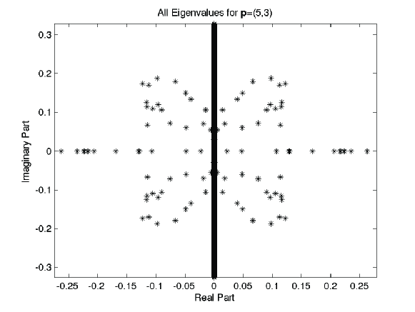
Figure 5.1. All eigenvalues for the case $\mathbf{p}=(5,3)^{T}$, $\Gamma=\frac{1}{2}$. The Zeitlin truncation is used with $N=200$. Note there are $200$ (or $100$ plus-minus pairs) eigenvalues with non-zero real part, and there are $100$ interior lattice points in $D_{\mathbf{p}}\setminus\{\mathbf{0}\}$. This confirms the result from [16]. Of the non-imaginary eigenvalues, $56$ are real and $144$ are complex. The number of interior points that satisfy $\rho_{0}<0$, $\rho_{1},\rho_{-1}>0$ is $24$. All these points correspond to real pairs (two sets of $24=48$). The other real pairs come from interior points with $\rho_{0}<0$ and $\rho_{1}<0$ or $\rho_{-1}<0$. This usually creates a complex quadruplet but in a few cases corresponds to two real pairs instead. Increasing $N$ does not change the number of non-imaginary eigenvalues.

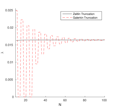
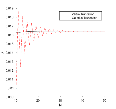
Figure 5.2. Numerically computed real eigenvalues vs Fourier mode domain size $N$.For these figure $\mathbf{a}=(0,3)^{T}$ and $\mathbf{p}=(3,1)^{T}$. The red dashed lines shows the eigenvalues computed by the Galerkin truncation in equation (2.29), and the black solid lines show the eigenvalues computed by the Zeitlin truncation in equation (2.30). For the left figure, the same truncation domain (2.7) is used for the Zeitlin truncation and the Galerkin truncation, meaning a larger matrix is computer for the Zeitlin truncation. For the right figure, a Galerkin truncation with $2N+1$ modes was chosen so that the same number of Fourier modes are included in both calculations. The convergence of the eigenvalue as a function of $N$ computed with the Zeitlin truncation is significantly better in either case. These plots omit the factor of $\alpha/\alpha^{\prime}$ for clarity.

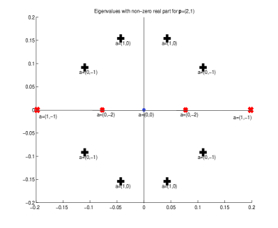
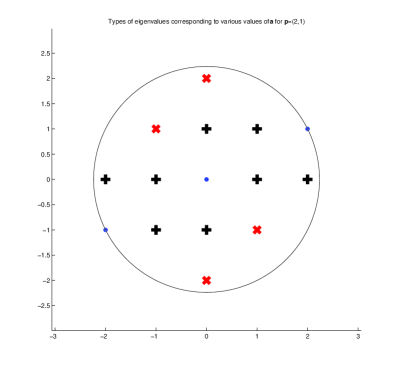
Figure 5.3. Non-imaginary eigenvalues (left) and the corresponding lattice points $\mathbf{a}$ in the unstable disc (right) for the equilibrium with $\mathbf{p}=(2,1)^{T}$. At the top, the eigenvalues with non-zero real part for every unstable class $\Sigma_{\mathbf{a}}$ are shown. Eigenvalues with zero imaginary part are marked with a red $\times$, complex eigenvalues are marked with a black $+$, and the zero eigenvalues are marked with a blue dot. In the bottom figure we see the values of $\mathbf{a}$ that correspond to these classes. The zero class led by $\mathbf{a}=(0,0)^{T}$ gives only zero eigenvalues. Compare the locations of the classes corresponding to real eigenvalues to the shaded region in figure 2.1. For these figures, $\Gamma=\frac{1}{2}$, so $\Omega^{*}=\cos(\mathbf{x}\cdot\mathbf{p})$, and a Zeitlin truncation is used for the approximation.

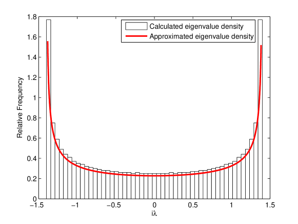
Figure 5.4. The density of the imaginary part of the spectrum, for the class $\mathbf{p}=(3,1)$, $\mathbf{a}=(1,-2)$, $N=1000$, and $\Gamma=0.5$. The bars show the normalized density of the imaginary eigenvalues computed for $N=1000$. The thick red line shows the approximate density computed by taking the approximation $\rho_{k}\to\frac{1}{|\mathbf{p}|^{2}}$. For this figure a Zeitlin truncation is used for the approximation.

5.1. The Unstable Spectrum

The Zeitlin class decomposition means that we now typically compute the eigenvalues of $(2N+1)$ matrices, each of size $(2N+1)\times(2N+1)$. Without the class decomposition, the eigenvalues of one $(2N+1)^{2}\times(2N+1)^{2}$ matrix need to be computed. So the class decomposition results in an extremely significant saving of computation time. For a Galerkin truncation, this computational saving is even more pronounced. However, this is at the expense of accuracy (see figure 5.2).

Figure 5.1 shows all the eigenvalues associated with a fixed value of $\mathbf{p}$ and $N$. There are exactly twice the number of interior lattice points in $D_{\mathbf{p}}\setminus{\mathbf{0}}$. This agrees with the result in [16] that the discrete spectrum of the corresponding operator has at most $2|D_{\mathbf{p}}|-2$ non-imaginary eigenvalues. Our numerical results indicate that this bound is likely to be sharp; for all choices of $\mathbf{p}$ tested there is equality.

Figure 5.2 shows the values at which the calculated eigenvalues converge as a function of the size $N$ of our truncation domain $\mathcal{D}$. Compared to the Galerkin truncation the eigenvalue converges for much smaller values of $N$ when using Zeitlin’s method.

Figure 5.3 shows the correspondence between the location of values of $\mathbf{a}$ and the types of eigenvalues of the class $\Sigma^{\prime}_{\mathbf{a}}$. This corresponds to the results of Section 3. Compare the positioning of the Fourier modes with figure 2.1.

5.2. The Stable Spectrum

Figure 5.4 shows the density of the imaginary parts of the spectrum for $\mathbf{a}=(-4,7)^{T}$, $\mathbf{p}=(7,5)^{T}$. There are also non-imaginary eigenvalues but these are not shown on the figure.

For any $\varepsilon>0$, we can choose sufficiently large $N$ so that there exists some $\mathbf{a}$ such that $\frac{1}{|{\mathbf{b}}|^{2}}<\varepsilon$ for all $\mathbf{b}\in\Sigma^{\prime}_{\mathbf{a}}$. So the imaginary spectrum of this class can be approximated by taking $\rho_{k}\approx\frac{1}{|\mathbf{p}|^{2}}$. The resulting matrix $A$ from (2.30) is now circulant. A circulant matrix is diagonalised by a discrete Fourier transform (see [13]). Thus the eigenvalues of $A$ are then found to be

(5.1) $$\lambda_{j}=\frac{2i}{|\mathbf{p}|^{2}}\sin\left(\frac{2\pi j}{n}\right)\text{ for }j=0,...,n-1\text{ where }j\text{ is the size of }A.$$

See [13] for details of this calculation.

Thus the approximate imaginary spectrum of $\Sigma_{\mathbf{a}}$ for sufficiently large $|\mathbf{a}|$ lies in the interval $\frac{2i}{|\mathbf{p}|^{2}}[-|\alpha|,|\alpha|]$ on the imaginary axis. Taking the limit $N\to\infty$ (and so $n\to\infty$), for each $x\in[0,1]$ there is a correspondence with an eigenvalue $\lambda_{x}$ where $x=\frac{1}{2\pi}\sin^{-1}\left(\frac{\lambda_{x}|\mathbf{p}|^{2}}{2i}\right)$. Differentiating this gives the density function

(5.2) $$F(x)=\frac{|\mathbf{p}|^{2}}{\pi\sqrt{4\alpha^{2}-|\mathbf{p}|^{4}x^{2}}}.$$

That is, the proportion of the eigenvalues lying between $c_{1}i$ and $c_{2}i$ on the imaginary axis is $\int_{c_{1}}^{c_{2}}F(x)\mathrm{d}x$ for $c_{1},c_{2}\in\frac{2}{|\mathbf{p}|^{2}}[-|\alpha|,|\alpha|]$. This curve is also plotted in 5.4, and it agrees well with the numerically calculated eigenvalues. This is surprising as the value of $|\mathbf{a}|$ is not particularly high. We can conclude that equation (5.2) gives a reasonable approximation of the imaginary spectrum for many choices of $\mathbf{a}$.

[16, 22] describe the essential spectrum of the linearised operator that coincides with our limit $N\to\infty$. The essential spectrum for the class led by $\mathbf{a}$ is given in that paper as

(5.3) $$\sigma_{\text{ess}}=i[-|\beta|,|\beta|],\text{ where }\beta=\frac{2}{|\mathbf{p}|^{2}}(\mathbf{a}\times\mathbf{p})\Gamma.$$

In the limit $N\to\infty$, $\frac{\sin(\varepsilon\mathbf{a}\times\mathbf{p})}{\varepsilon}\to\mathbf{a}\times\mathbf{p}$, so $\frac{2}{|\mathbf{p}|^{2}}|\alpha|\to|\beta|$. Thus our approximation for large $N$ reproduces the essential spectrum of a single class calculated in [16]. Note that this is the essential spectrum associated with a single subsystem of the linearised problem. The essential spectrum of the full system is the superposition of all these essential spectra. It was shown in [22] that this is $i\mathds{R}$, which follows from considering the superposition of (5.3) for all possible values of $\mathbf{a}$.

6. Conclusion

We have demonstrated the non-linear instability of the stationary solutions with vorticity $\Omega^{*}=2\Gamma\cos(\mathbf{p}\cdot\mathbf{x})$ in the Euler equations for almost all values of $\mathbf{p}$ such that $\mathbf{p}\neq(1,0)^{T}$ (or rotations and reflections thereof). We started out by using the Zeitlin truncation, and observe the numerical approximation of eigenvalues for finite $N$ obtained from Zeitlin’s truncation converge much faster with $N$. However, the Zeitlin truncation does not behave well when $\text{gcd}(p_{1},p_{2})$ is even. Because of this, we developed much of our theory for both truncations.

In addition, we have recreated and extended a number of results described by [17], [16], and [22]. Specifically, we have shown that the “unstable disc theorem” presented in [17] still holds true in the current context of finite dimensional approximation. Moreover, we have shown that for almost all $\mathbf{p}$ we can use the unstable disc to prove instability (as opposed to the existing stability results developed by Li and others). We have also numerically verified the bound on the number of non-imaginary eigenvalues and the essential spectrum of an individual class in [16] and [22]. We used very different approaches and arguments to those papers.

There are obvious extensions of this work. The first is a complete description of the non-imaginary spectrum. This would require first showing that for two consecutive negative values of $\rho$, the corresponding subsystem has four non-imaginary eigenvalues, either two real pairs or a complex quadruplet. This would be a step towards proving that the bound from [16] is sharp. Another extension would be to see if any of the methods used in this paper could be applied to more complex steady states, for instance $\Omega^{*}=\sin(p_{1}x)\sin(p_{2}y)$.

A similar analysis of the Euler fluid equations on a three dimensional torus would be interesting. A Zeitlin-style structure preserving truncation for the 3D case is not possible, as the Casimirs that make such a truncation useful are not present in the 3D problem[24]. Similar stability results may still be possible using a Galerkin style truncation instead.

There is also a discussion of a structure-preserving truncation that includes a viscosity term in [26]. A comparison of Zeitlin’s truncation to standard truncations with a viscosity term included as in Figure 5.2 would be valuable.

A significant extension of this material would be an application of the same methods to the Euler problem on a sphere. There similar structure preserving truncation also due to Zeitlin for the sphere [25] and so there is some hope of similar results in that setting.

References

• [1] V.I. Arnold. Mathematical Methods of Classical Mechanics. Springer, 1978.
• [2] V.I. Arnold and Boris A. Khesin. Topological Methods in Hydrodynamics. Springer, 1998.
• [3] Vladimir Arnold. Sur la géométrie différentielle des groupes de lie de dimension infinie et ses applications à l’hydrodynamique des fluides parfaits. In Annales de l’institut Fourier, volume 16, pages 319–361. Institut Fourier, 1966.
• [4] Margaret Beck and C. Eugene Wayne. Metastability and rapid convergence to quasi-stationary bar states for the two-dimensional navier-stokes equations. Proceedings of the Royal Society of Edinburgh Section A - Mathematics, 143(5):905–927, 2013.
• [5] L Belenkaya, S Friedlander, and V Yudovich. The unstable spectrum of oscillating shear flows. SIAM Journal on Applied Mathematics, 59(5):1701–1715, 1999.
• [6] Martin Bordemann, Jens Hoppe, Peter Schaller, and Martin Schlichenmaier. $gl(\infty)$ and geometric quantization. Communications in Mathematical Physics, 138(2):209–244, 1991.
• [7] P. Butta and P. Negrini. On the stability problem of stationary solutions for the Euler equation on a 2-dimensional torus. Regular and Chaotic Dynamics, 15(6):637–645, 2010.
• [8] Ana Cannas da Silva. Lectures on Symplectic Geometry. Springer, 2001.
• [9] Jean Favard. Sur les polynomes de Tchebicheff. Comptes Rendus de l’Académie des Sciences, 200:2052–2053, 1936.
• [10] Susan Friedlander, Walter Strauss, and Misha Vishik. Nonlinear instability in an ideal fluid. In Annales de l’Institut Henri Poincare (C) Non Linear Analysis, volume 14, pages 187–209. Elsevier, 1997.
• [11] Dan Henry. Geometric theory of semilinear parabolic equations. LNM 840. Springer, 1981.
• [12] Jens Hoppe. Diffeomorphism groups, quantization, and $su(\infty)$. International Journal of Modern Physics A, 4(19):5235–5248, 1989.
• [13] Herbert Karner, Josef Schneid, and Christoph W. Ueberhuber. Spectral decomposition of real circulant matrices. Linear Algebra and its Applications, 367:301–311, 2002.
• [14] Boris Kolev. Poisson brackets in hydrodynamics. Discrete and Continuous Dynamical Systems, 19:555–574, 2007.
• [15] Yueheng Lan and Y Charles Li. On the dynamics of navier-stokes and euler equations. Journal of Statistical Physics, 132(1):35–76, 2008.
• [16] Y. Latushkin, Y. C. Li, and M. Stanislavova. The spectrum of a linearized 2D Euler operator. Studies in Applied Mathematics, 112:259–270, 2004.
• [17] Yanguang (Charles) Li. On 2D Euler equations. I. On the energy-casimir stabilities and the spectra for linearized 2D euler equations. Journal of Mathematical Physics, 41(2):728 – 758, 2000.
• [18] Guriĭ Ivanovich Marchuk and Jiri Ruzicka. Methods of numerical mathematics, volume 2. Springer-Verlag New York, 1975.
• [19] LD Meshalkin and Ia G Sinai. Investigation of the stability of a stationary solution of a system of equations for the plane movement of an incompressible viscous liquid. Journal of Applied Mathematics and Mechanics, 25(6):1700–1705, 1961.
• [20] C N Pope and L J Romans. Local area-preserving algebras for two-dimensional surfaces. Classical and Quantum Gravity, 7:97–109, 1990.
• [21] Samriddhi Sankar Ray, Uriel Frisch, Sergei Nazarenko, and Takeshi Matsumoto. Resonance phenomenon for the Galerkin-truncated Burgers and Euler equations. Physics Review E, 84, 2011.
• [22] Roman Shvidkoy and Yuri Latushkin. The essential spectrum of the linearized 2d euler operator is a vertical band. Contemporary Mathematics, 327:299–304, 2003.
• [23] Gábor Szegő. Orthogonal Polynomials. American Mathematical Society, 1939.
• [24] V. Zeitlin. Finite-mode analogs of 2D ideal hydrodynamics: Coadjoint orbits and local canonical structure. Physica D: Nonlinear Phenomena, 49(3):353–362, 1991.
• [25] V Zeitlin. Self-consistent finite-mode approximations for the hydrodynamics of an incompressible fluid on nonrotating and rotating spheres. Physical review letters, 93(26):264501, 2004.
• [26] V. Zeitlin. On self-consistent finite-mode approximations in (quasi-)two-dimensional hydrodynamics and magnetohydrodynamics. Physics Letters A, 339:316–324, 2005.