Local zeta regularization   and the scalar Casimir effect III.   The case with a background harmonic potential

Davide Fermi$\,{}^{a}$, Livio Pizzocchero$\,{}^{b}$()

^a Dipartimento di Matematica, Università di Milano

Via C. Saldini 50, I-20133 Milano, Italy

e–mail: davide.fermi@unimi.it

^b Dipartimento di Matematica, Università di Milano

Via C. Saldini 50, I-20133 Milano, Italy

and Istituto Nazionale di Fisica Nucleare, Sezione di Milano, Italy

e–mail: livio.pizzocchero@unimi.it

Applying the general framework for local zeta regularization proposed in Part I of this series of papers, we renormalize the vacuum expectation value of the stress-energy tensor (and of the total energy) for a scalar field in presence of an external harmonic potential.

Keywords: Local Casimir effect, renormalization, zeta regularization.

AMS Subject classifications: 81T55, 83C47.

PACS: 03.70.+k, 11.10.Gh, 41.20.Cv .

1 Introduction

In Part I of this series of papers [10, 11, 12] (partly inspired by [9]) we have considered the general framework of local (and global) zeta regularization of a neutral scalar field in a $d$-dimensional spatial domain $\Omega$, in the environment of $(d+1)$-dimensional Minkowski spacetime; the possible presence of an external potential $V$ was taken into account as well.

In the present Part III we consider a massless field on $\Omega={\bf R}^{d}$, and choose for $V$ a harmonic potential. The potential is assumed to be isotropic, i.e., to be proportional to the squared radius $|{\bf x}|^{2}$ (${\bf x}\in{\bf R}^{d}$); nevertheless, our approach could be extended with little effort to anisotropic harmonic potentials and to the case of a massive scalar field.

The main result of this paper is the renormalization of the vacuum expectation value (VEV) for the stress-energy tensor, obtained applying the general framework of Part I to the present configuration; we also discuss the total energy in this configuration. After producing general integral representations for both the renormalized stress-energy VEV and the total energy, we consider in detail the cases of spatial dimension $d\in\{1,2,3\}$.

The above mentioned integral representations are derived analytically and are fully explicit; however, the integrals therein must be computed numerically. We have performed these latter computations for $d\in\{1,2,3\}$, using $\tt{Mathematica}$.

Using the previously cited integral representation, it is also possible to derive the asymptotics for the stress-energy tensor components when the radius $|{\bf x}|$ goes to zero or to infinity; we derive, as well, remainder estimates for these asymptotic expansions as well.

The idea to replace sharp boundaries with suitable background potentials is well-known in the literature on the Casimir effect. Typically (see, e.g., [3, 5, 15, 17, 19]), delta-like potentials are introduced in order to mimic boundary conditions in a “physically more realistic” framework; the ultimate purpose is to obtain less singular behaviours of the renormalized quantities, avoiding, e.g., boundary divergences such as the ones pointed out in Parts I and II [10, 11]. The case of a scalar field interacting with an external harmonic potential has been formerly considered by Actor and Bender [1, 2], who have determined the renormalized VEV of the total energy via global zeta regularization; to the best of our knowledge, local aspects such as the stress-energy tensor have never been considered previously for the present configuration.

The paper is organized as follows. In Section 2 we present a summary of basic results from Part I; as in Part II, the purpose of the summary is to save the reader from the tedious task of recovering from Part I the general identities applied here. In Section 3 (and in the related Appendix A) we discuss the general approach to treat the case of a scalar field interacting with a classical, isotropic harmonic potential in arbitrary spatial dimension $d$; this includes general expressions for the renormalized stress-energy VEV, its asymptotics for $|{\bf x}|$ small or large and for the renormalized VEV of the total energy (more precisely, for the bulk energy as defined in Part I). The main ingredients in the derivation of the above results are:

i) the general results of Part I relating the zeta regularization to the heat kernel of fundamental operator ${\mathcal{A}}=-\Delta+V({\bf x})$;

ii) the fact that, when $V({\bf x})$ is harmonic, the related heat kernel is the well-known Mehler kernel [18] (also see [4, 6, 8, 16]).

In Section 4, the analysis presented in the preceeding sections is specified to the cases of spatial dimension $d\in\{1,2,3\}$.

We point out that results on the renormalized bulk energy agree with the ones of Actor and Bender [2] for $d\in\{1,2,3\}$. Nevertheless, it should be mentioned that these authors compute the analytic continuations required by the zeta approach using ad hoc results on continuation the special functions involved in this specific case; on the contrary, here we are applying mechanically the general setting discussed in Part I, in the spirit of the present series of papers.

2 A summary of results from Part I

2.1   General setting.

Throughout the paper we use natural units, so that

$$c=1~{},\qquad\hbar=1~{}.$$ (2.1)

Our approach works in $(d+1)$-dimensional Minkowski spacetime, which is identified with ${\bf R}^{d+1}$ using a set of inertial coordinates

$$x=(x^{\mu})_{\mu=0,1,...,d}\equiv(x^{0},{\bf x})\equiv(t,{\bf x})~{};$$ (2.2)

the Minkowski metric is $(\eta_{\mu\nu})=\mbox{diag}(-1,1,...\,,1)$ . We fix a spatial domain $\Omega\subset{\bf R}^{d}$ and a background static potential $V\!:\!\Omega\!\to\!{\bf R}$. We consider a quantized neutral, scalar field $\widehat{\phi}:{\bf R}\times\Omega\to{\mathcal{L}}_{sa}(\mathfrak{F})$ ($\mathfrak{F}$ is the Fock space and ${\mathcal{L}}_{sa}(\mathfrak{F})$ are the selfadjoint operators on it); suitable boundary conditions are prescribed on $\partial\Omega$. The field equation reads

$$0=(-\partial_{tt}+\Delta-V({\bf x}))\widehat{\phi}({\bf x},t)$$ (2.3)

($\Delta:=\sum_{i=1}^{d}\partial_{ii}$ is the $d$-dimensional Laplacian). We put

$${\mathcal{A}}:=-\Delta+V~{},$$ (2.4)

keeping into account the boundary conditions on $\partial\Omega$, and consider the Hilbert space $L^{2}(\Omega)$ with inner product $\langle f|g\rangle:=\int_{\Omega}d{\bf x}\,\overline{f}({\bf x})g({\bf x})$. We assume ${\mathcal{A}}$ to be selfadjoint in $L^{2}(\Omega)$ and strictly positive (i.e., with spectrum $\sigma({\mathcal{A}})\subset[\varepsilon^{2},+\infty)$ for some $\varepsilon>0$).

We often refer to a complete orthonormal set $(F_{k})_{k\in{\mathcal{K}}}$ of (proper or improper) eigenfunctions of ${\mathcal{A}}$ with eigenvalues $(\omega^{2}_{k})_{k\in{\mathcal{K}}}$ ($\omega_{k}\!\geqslant\!\varepsilon$ for all $k\!\in\!{\mathcal{K}}$). Thus

$$\begin{split}&F_{k}:\Omega\to{\bf C};\qquad{\mathcal{A}}F_{k}=\omega^{2}_{k}F_{k}~{};\\ &\langle F_{k}|F_{h}\rangle=\delta(k,h)\quad\mbox{for all $k,h\in{\mathcal{K}}$}~{}.\end{split}$$ (2.5)

The labels $k\!\in\!{\mathcal{K}}$ can include both discrete and continuous parameters; $\int_{\mathcal{K}}dk$ indicates summation over all labels and $\delta(h,k)$ is the Dirac delta function on ${\mathcal{K}}$.

We expand the field $\widehat{\phi}$ in terms of destruction and creation operators corresponding to the above eigenfunctions, and assume the canonical commutation relations; $|0\rangle\in\mathfrak{F}$ is the vacuum state and VEV stands for “vacuum expectation value”.

The quantized stress-energy tensor reads ($\xi\!\in\!{\bf R}$ is a parameter)

$$\widehat{T}_{\mu\nu}:=\left(1-2\xi\right)\partial_{\mu}\widehat{\phi}\circ\partial_{\nu}\widehat{\phi}-\left({1\over 2}-2\xi\right)\eta_{\mu\nu}(\partial^{\lambda}\widehat{\phi}\,\partial_{\lambda}\widehat{\phi}+V\widehat{\phi}^{2})-2\xi\,\widehat{\phi}\circ\partial_{\mu\nu}\widehat{\phi}\,;$$ (2.6)

in the above we put $\widehat{A}\circ\widehat{B}:=(1/2)(\widehat{A}\widehat{B}+\widehat{B}\widehat{A})$ for all $\widehat{A},\widehat{B}\in{\mathcal{L}}_{sa}(\mathfrak{F})$, and all the bilinear terms in the field are evaluated on the diagonal (e.g., $\partial_{\mu}\widehat{\phi}\circ\partial_{\nu}\widehat{\phi}$ indicates the map $x\mapsto\partial_{\mu}\widehat{\phi}(x)\circ\partial_{\nu}\widehat{\phi}(x)$). The VEV $\langle 0|\widehat{T}_{\mu\nu}|0\rangle$ is typically divergent.

2.2   Zeta regularization.

The zeta-regularized field operator is

$$\widehat{\phi}^{u}:=(\kappa^{-2}{\mathcal{A}})^{-u/4}\widehat{\phi}~{},$$ (2.7)

where ${\mathcal{A}}$ is the operator (2.4), $u\in{\bf C}$ and $\kappa>0$ is a “mass scale” parameter; note that $\widehat{\phi}^{u}|_{u=0}=\widehat{\phi}$, at least formally. The zeta regularized stress-energy tensor is

$$\widehat{T}^{u}_{\mu\nu}:=(1\!-\!2\xi)\partial_{\mu}\widehat{\phi}^{u}\!\circ\partial_{\nu}\widehat{\phi}^{u}\!-\!\left({1\over 2}\!-\!2\xi\!\right)\!\eta_{\mu\nu}\!\left(\!\partial^{\lambda}\widehat{\phi}^{u}\partial_{\lambda}\widehat{\phi}^{u}\!+\!V(\widehat{\phi}^{u})^{2}\right)-2\xi\,\widehat{\phi}^{u}\!\circ\partial_{\mu\nu}\widehat{\phi}^{u}\,.$$ (2.8)

The VEV $\langle 0|\widehat{T}^{u}_{\mu\nu}|0\rangle$ is well defined for $\Re u$ large enough (see the forthcoming subsection 2.5); moreover, in the region of definition it is an analytic function of $u$. The same can be said of many related observables (including global objects, such as the total energy VEV).

For any one of these observables, let us denote with ${\mathcal{F}}(u)$ its zeta-regularized version and assume this to be analytic for $u$ in a suitable domain ${\mathcal{U}}_{0}\subset{\bf C}$. The zeta approach to renormalization can be formulated in two versions.

i) Restricted version. Assume the map ${\mathcal{U}}_{0}\!\to\!{\bf C}$, $u\!\mapsto\!{\mathcal{F}}(u)$ to admit an analytic continuation (indicated with the same notation) to an open subset ${\mathcal{U}}\!\subset\!{\bf C}$ with ${\mathcal{U}}\!\ni\!0$ ; then we define the renormalized observables as

$${\mathcal{F}}_{ren}:={\mathcal{F}}(0)~{}.$$ (2.9)

ii) Extended version. Assume that there exists an open subset ${\mathcal{U}}\!\subset\!{\bf C}$ with ${\mathcal{U}}_{0}\!\subset\!{\mathcal{U}}$, such that $0\!\in\!{\mathcal{U}}$ and the map $u\!\in\!{\mathcal{U}}_{0}\mapsto{\mathcal{F}}(u)$ has an analytic continuation to ${\mathcal{U}}\!\setminus\!\{0\}$ (still denoted with ${\mathcal{F}}$). Starting from the Laurent expansion ${\mathcal{F}}(u)=\sum_{k=-\infty}^{+\infty}{\mathcal{F}}_{k}u^{k}$, we introduce the regular part $(RP\,{\mathcal{F}})(u):=\sum_{k=0}^{+\infty}{\mathcal{F}}_{k}u^{k}$ and define

$${\mathcal{F}}_{ren}:=(RP\,{\mathcal{F}})(0)~{}.$$ (2.10)

Of course, if ${\mathcal{F}}$ is regular at $u=0$ the defnitions (2.9) (2.10) coincide.

In the case of the stress-energy VEV, the prescriptions (i) and (ii) read, respectively,

$$\langle 0|\widehat{T}_{\mu\nu}(x)|0\rangle_{ren}:=\langle 0|\widehat{T}^{u}_{\mu\nu}(x)|0\rangle\Big{|}_{u=0}~{},$$ (2.11)

$$\langle 0|\widehat{T}_{\mu\nu}(x)|0\rangle_{ren}:=RP\Big{|}_{u=0}\langle 0|\widehat{T}^{u}_{\mu\nu}(x)|0\rangle~{}.$$ (2.12)

2.3   Conformal and non-conformal parts of the stress-energy VEV.

These are indicated by the superscripts $(\lozenge)$ and $(\blacksquare)$, respectively; they are defined by

$$\langle 0|\widehat{T}_{\mu\nu}|0\rangle_{ren}=\langle 0|\widehat{T}^{(\lozenge)}_{\mu\nu}|0\rangle_{ren}+(\xi\!-\!\xi_{d})\,\langle 0|\widehat{T}^{(\blacksquare)}_{\mu\nu}|0\rangle_{ren}~{},$$ (2.13)

where we are considering for the parameter $\xi$ the critical value

$$\xi_{d}:={d\!-\!1\over 4d}~{}.$$ (2.14)

2.4   Integral kernels.

If ${\mathcal{B}}$ is a linear operator in $L^{2}(\Omega)$, its integral kernel is the (generalized) function $({\bf x},{\bf y})\in\Omega\!\times\!\Omega\mapsto{\mathcal{B}}({\bf x},{\bf y}):=\langle\delta_{{\bf x}}|{\mathcal{B}}\,\delta_{{\bf y}}\rangle$ ($\delta_{\bf x}$ is the Dirac delta at ${\bf x}$). The trace of ${\mathcal{B}}$, assuming it exists, fulfills $\mbox{Tr}\,{\mathcal{B}}=\int_{\Omega}d{\bf x}\,{\mathcal{B}}({\bf x},{\bf x})$ .

In the following subsections ${\mathcal{A}}$ is a strictly positive selfadjoint operator in $L^{2}(\Omega)$, with a complete orthonormal set of eigenfunctions as in Eq. (2.5). In typical applications, ${\mathcal{A}}$ is the operator (2.4).

2.5   The Dirichlet kernel and its relations with the stress-energy VEV.

For (suitable) $s\in{\bf C}$, the $s$-th Dirichlet kernel of ${\mathcal{A}}$ is

$$D_{s}({\bf x},{\bf y}):={\mathcal{A}}^{-s}({\bf x},{\bf y})=\int_{\mathcal{K}}{dk\over\omega_{k}^{2s}}\;F_{k}({\bf x})\overline{F_{k}}({\bf y})~{}.$$ (2.15)

If ${\mathcal{A}}=-\Delta+V$ (with $V$ a smooth potential) is strictly positive, the map $D_{s}(~{},~{}):\Omega\times\Omega\to{\bf C}$, $({\bf x},{\bf y})\mapsto D_{s}({\bf x},{\bf y})$ is continuous along with all its partial derivatives up to order $j\in{\bf N}$, for all $s\in{\bf C}$ with $\Re s>d/2+j/2$ . Recalling Eq. (2.8), the regularized stress-energy VEV can be expressed as follows:

$${~{}}\langle 0|\widehat{T}^{u}_{00}({\bf x})|0\rangle\!=\!\kappa^{u}\!\left[\!\left(\!\frac{1}{4}\!+\!\xi\!\right)\!D_{{u-1\over 2}}({\bf x},{\bf y})\!+\!\left(\!\frac{1}{4}\!-\!\xi\!\right)\!(\partial^{x^{\ell}}\!\partial_{y^{\ell}}\!+\!V({\bf x}))D_{{u+1\over 2}}({\bf x},{\bf y})\right]_{{\bf y}={\bf x}}\!,$$ (2.16)

$$\langle 0|\widehat{T}^{u}_{0j}({\bf x})|0\rangle=\langle 0|\widehat{T}^{u}_{j0}({\bf x})|0\rangle=0~{},$$ (2.17)

$$\begin{split}&{~{}}\hskip 108.12054pt\langle 0|\widehat{T}^{u}_{ij}({\bf x})|0\rangle=\langle 0|\widehat{T}^{u}_{ji}({\bf x})|0\rangle=\\ &=\kappa^{u}\!\left[\!\Big{(}{1\over 4}-\xi\Big{)}\delta_{ij}\Big{(}\!D_{{u-1\over 2}}({\bf x},{\bf y})-(\partial^{\,x^{\ell}}\!\partial_{y^{\ell}}\!+\!V({\bf x}))D_{{u+1\over 2}}({\bf x},{\bf y})\Big{)}\,+\right.\\ &\hskip 142.26378pt\left.+\left(\!\Big{(}{1\over 2}-\xi\Big{)}\partial_{x^{i}y^{j}}-\xi\,\partial_{x^{i}x^{j}}\!\right)\!D_{{u+1\over 2}}({\bf x},{\bf y})\right]_{{\bf y}={\bf x}}\end{split}$$ (2.18)

($\langle 0|\widehat{T}^{u}_{\mu\nu}({\bf x})|0\rangle$ is short for $\langle 0|\widehat{T}^{u}_{\mu\nu}(t,{\bf x})|0\rangle$; indeed, the VEV does not depend on $t$); of course, the map $\Omega\to{\bf C}$, ${\bf x}\mapsto\langle 0|\widehat{T}^{u}_{\mu\nu}({\bf x})|0\rangle$ possesses the same regularity as the functions ${\bf x}\in\Omega\mapsto D_{u\pm 1\over 2}({\bf x},{\bf x}),\partial_{zw}D_{u+1\over 2}({\bf x},{\bf x})$ ($z,w$ any two spatial variables); so, due to the previously mentioned results, ${\bf x}\mapsto\langle 0|\widehat{T}^{u}_{\mu\nu}({\bf x})|0\rangle$ is continuous for $\Re u>d+1$.

The above framework relates the renormalized stress-energy VEV $\langle 0|\widehat{T}_{\mu\nu}({\bf x})|0\rangle_{ren}:=RP|_{u=0}\langle 0|\widehat{T}^{u}_{\mu\nu}({\bf x})|0\rangle$ to the analytic continuation at $u=0$ of the maps $u\mapsto\kappa^{u}D_{u\pm 1\over 2}({\bf x},{\bf y})$ and of their derivatives.

In the sequel we will also consider the total energy VEV and express it in terms of the trace $\mbox{Tr}\,{\mathcal{A}}^{-s}$, fulfilling

$$\mbox{Tr}\,{\mathcal{A}}^{-s}=\int_{\Omega}d{\bf x}\;D_{s}({\bf x},{\bf x})~{}.$$ (2.19)

2.6   The heat kernel.

For $\mathfrak{t}\in[0,+\infty)$, this is given by

$$K(\mathfrak{t}\,;{\bf x},{\bf y}):=e^{-\mathfrak{t}{\mathcal{A}}}({\bf x},{\bf y})=\int_{\mathcal{K}}dk\;e^{-\mathfrak{t}\,\omega_{k}^{2}}\,F_{k}({\bf x})\overline{F_{k}}({\bf y})~{}.$$ (2.20)

If ${\mathcal{A}}=-\Delta+V$ ($V$ smooth) is strictly positive, the map $K(\mathfrak{t}\,;~{},~{}):\Omega\times\Omega\to{\bf C}$, $({\bf x},{\bf y})\mapsto K(\mathfrak{t}\,;{\bf x},{\bf y})$ is continuous along with all its partial derivatives of any order, for all $\mathfrak{t}>0$ . The heat trace (assuming it to exists) is

$$K(\mathfrak{t}):=\mbox{Tr}\,e^{-\mathfrak{t}{\mathcal{A}}}=\int_{\Omega}d{\bf x}\;K(\mathfrak{t}\,;{\bf x},{\bf x})~{}.$$ (2.21)

2.7   The Dirichlet kernel as Mellin transform of the heat kernel.

For suitable values of $s\!\in\!{\bf C}$ (see Part I), there holds

$$D_{s}({\bf x},{\bf y})={1\over\Gamma(s)}\int_{0}^{+\infty}\!d\mathfrak{t}\;\mathfrak{t}^{s-1}\,K(\mathfrak{t}\,;{\bf x},{\bf y})~{}.$$ (2.22)

Similar results hold for $\mbox{Tr}\,{\mathcal{A}}^{-s}$; for example, using the heat trace $K(\mathfrak{t})$ of Eq. (2.21), we obtain

$$\mbox{Tr}\,{\mathcal{A}}^{-s}={1\over\Gamma(s)}\int_{0}^{+\infty}\!d\mathfrak{t}\;\mathfrak{t}^{s-1}\,K(\mathfrak{t})~{}.$$ (2.23)

2.8   Analytic continuation of Mellin transforms via integration by parts.

Let $\mathcal{F}:(0,+\infty)\to{\bf C}$ be a function of the form

$$\mathcal{F}(\mathfrak{t})={1\over\mathfrak{t}^{\rho}}\,\mathcal{H}(\mathfrak{t})$$ (2.24)

for some $\rho\in{\bf C}$ and some smooth function $\mathcal{H}:[0,+\infty)\to{\bf C}$, vanishing exponentially for $\mathfrak{t}\to+\infty$. Consider the Mellin transform of $\mathcal{F}$, i.e.

$$\mathfrak{M}(\sigma):=\int_{0}^{+\infty}\!\!d\mathfrak{t}\;\mathfrak{t}^{\sigma-1}\,\mathcal{F}(\mathfrak{t})~{};$$ (2.25)

this is an analytic function of $\sigma$ for $\Re\sigma>\Re\rho$. Integrating the above equation by parts $n$ times (for any $n\in\{1,2,3,...\}$) we obtain the relation

$$\mathfrak{M}(\sigma)={(-1)^{n}\over(\sigma\!-\!\rho)...(\sigma\!-\!\rho\!+\!n\!-\!1)}\int_{0}^{+\infty}\!\!d\mathfrak{t}\;\mathfrak{t}^{\sigma-\rho+n-1}\,{d^{n}\mathcal{H}\over d\mathfrak{t}^{n}}(\mathfrak{t})~{},$$ (2.26)

giving the analytic continuation of $\mathfrak{M}(\sigma)$ to a meromorphic function of $\sigma$ in the region $\{\Re\sigma>\Re\rho-n\}$, possibly with simple poles at $\sigma\in\{\rho\,,\,\rho-1\,,\,...\,,\,\rho-n+1\}$.

The above results can be employed to obtain the analytic continuations of the regularized stress-energy VEV $\langle 0|\widehat{T}^{u}_{\mu\nu}({\bf x})|0\rangle$ (treating ${\bf x}\in\Omega$ as a fixed parameter) and of the trace $\mbox{Tr}\,{\mathcal{A}}^{-s}$; for example, assuming the heat trace $K(\mathfrak{t})$ to have the form

$$K(\mathfrak{t})={1\over\mathfrak{t}^{p}}\;H(\mathfrak{t})~{},$$ (2.27)

for some $p\in{\bf R}$ and some smooth function $H:[0,+\infty)\to{\bf R}$, vanishing rapidly for $\mathfrak{t}\to+\infty$, starting from Eq. (2.23) we obtain (for $n\in\{1,2,3,...\}$)

$$\mbox{Tr}\,{\mathcal{A}}^{-s}={(-1)^{n}\over\Gamma(s)(s\!-\!p)...(s\!-\!p\!+\!n\!-\!1)}\int_{0}^{+\infty}\!\!d\mathfrak{t}\;\mathfrak{t}^{s-p+n-1}\,{d^{n}H\over d\mathfrak{t}^{n}}(\mathfrak{t})~{}.$$ (2.28)

2.9   The case of product domains. Factorization of the heat kernel.

Let ${\mathcal{A}}:=-\Delta+V$ and consider the case where

$$\Omega=\Omega_{1}\times\Omega_{2}\ni{\bf x}=({\bf x}_{1},{\bf x}_{2})\,,{\bf y}=({\bf y}_{1},{\bf y}_{2})~{},$$ (2.29)

$$V({\bf x})=V_{1}({\bf x}_{1})+V_{2}({\bf x}_{2})$$ (2.30)

($\Omega_{a}\!\subset\!{\bf R}^{d_{a}}$ is an open subset, for $a\in\{1,2\}$; $d_{1}\!+\!d_{2}=d$); assume the boundary conditions on $\partial\Omega$ to arise from suitable boundary conditions prescribed separately on $\partial\Omega_{1}$ and $\partial\Omega_{2}$ so that, for $a=1,2$, the operators

$${\mathcal{A}}_{a}:=-\Delta_{a}+V({\bf x}_{a})$$ (2.31)

(with $\Delta_{a}$ the Laplacian on $\Omega_{a}$) are selfadjoint and strictly positive in $L^{2}(\Omega_{a})$. Then, the Hilbert space $L^{2}(\Omega)$ and the operator ${\mathcal{A}}$ can be represented as

$$L^{2}(\Omega)=L^{2}(\Omega_{1})\otimes L^{2}(\Omega_{2})~{},\qquad{\mathcal{A}}={\mathcal{A}}_{1}\otimes\mbox{{1}}+\mbox{{1}}\otimes{\mathcal{A}}_{2}~{}.$$ (2.32)

This implies, amongst else, that the heat kernels $K(\mathfrak{t}\,;{\bf x},{\bf y}):=e^{\mathfrak{t}{\mathcal{A}}}({\bf x},{\bf y})$, $K_{a}(\mathfrak{t}\,;{\bf x}_{a},{\bf y}_{a})$ $:=e^{\mathfrak{t}{\mathcal{A}}_{a}}({\bf x}_{a},{\bf y}_{a})$ ($a=1,2$) are related by

$$K(\mathfrak{t}\,;{\bf x},{\bf y})=K_{1}(\mathfrak{t}\,;{\bf x}_{1},{\bf y}_{1})\,K_{2}(\mathfrak{t}\,;{\bf x}_{1},{\bf x}_{2})~{}.$$ (2.33)

Similarly, writing $K(\mathfrak{t})$, $K_{a}(\mathfrak{t})$ ($a\in\{1,2\}$) for the heat traces of ${\mathcal{A}}$ and ${\mathcal{A}}_{a}$ ($a\in\{1,2\}$), respectively, we have

$$K(\mathfrak{t})=K_{1}(\mathfrak{t})\,K_{2}(\mathfrak{t})~{}.$$ (2.34)

Let us briefly recall that a special subcase of the present framework is the case of a slab, i.e.,

$$\Omega=\Omega_{1}\times{\bf R}^{d_{2}}\ni{\bf x}=({\bf x}_{1},{\bf x}_{2})\,,{\bf y}=({\bf y}_{1},{\bf y}_{2})~{},\qquad V({\bf x})=V({\bf x}_{1})$$ (2.35)

with $\Omega_{1}\subset{\bf R}^{d_{1}}$ an open subset ($d_{1}\!+\!d_{2}=d$); see Part I for more details on this topic.
  

2.10   The total energy.

The zeta-regularized total energy is

$${\mathcal{E}}^{u}:=\int_{\Omega}d{\bf x}\;\langle 0|\widehat{T}^{u}_{00}({\bf x})|0\rangle=E^{u}+B^{u}~{};$$ (2.36)

the second equality is proved after defining the regularized bulk and boundary energies, which are

$$E^{u}:={\kappa^{u}\!\over 2}\int_{\Omega}d{\bf x}\;D_{{u-1\over 2}}({\bf x},{\bf x})={\kappa^{u}\!\over 2}\;\mbox{Tr}\,\,{\mathcal{A}}^{{1-u\over 2}}~{},$$ (2.37)

$$B^{u}:=\kappa^{u}\left(\!{1\over 4}-\xi\!\right)\!\int_{\partial\Omega}\!da({\bf x})\,\left.{\partial\over\partial n_{{\bf y}}}\,D_{{u+1\over 2}}({\bf x},{\bf y})\right|_{{\bf y}={\bf x}}~{}.$$ (2.38)

If $\Omega$ is unbounded, the integral over $\partial\Omega$ in Eq. (2.38) has to be intended as $\lim_{\ell\to+\infty}\int_{\partial\Omega_{\ell}}da$, where $(\Omega_{\ell})_{\ell=0,1,2,...}$ is a sequence of bounded subdomains with $\Omega_{\ell}\subset\Omega_{\ell+1}$ for $\ell\in\{0,1,2,..\}$, and $\cup_{\ell=0}^{+\infty}\Omega_{\ell}=\Omega$.

Assuming $E^{u}$ and $B^{u}$ (see Eq.s (2.37) (2.38)) to be finite and analytic for suitable $u\in{\bf C}$, we define the renormalized energies by the generalized (or restricted) zeta approach; for example, we put

$$E^{ren}:=RP\Big{|}_{u=0}E^{u}\qquad\left(\mbox{or }\;E^{ren}:=E^{u}\Big{|}_{u=0}\,\right)\,.$$ (2.39)

2.11   Curvilinear coordinates.

In some applications it is natural to employ on $\Omega$ some set of curvilinear coordinates $(q^{i})_{i=1,...,d}\equiv{\bf q}$, inducing a set of spacetime coordinates $q\equiv(q^{\mu})\equiv(t,{\bf q})$; the spatial and space-time line elements are, respectively,

$$\begin{split}&\hskip 34.14322ptd\ell^{2}=a_{ij}({\bf q})dq^{i}dq^{j}~{};\qquad ds^{2}=-dt^{2}\!+\!d\ell^{2}=g_{\mu\nu}(q)\,dq^{\mu}dq^{\nu}~{},\\ &g_{00}:=-1~{},~{}\quad g_{i0}=g_{0i}:=0~{},~{}\quad g_{ij}(q):=a_{ij}({\bf q})\qquad\mbox{for $i,j\in\{1,...,d\}$}~{}.\end{split}$$ (2.40)

The analogue of Eq. (2.8) in the coordinate system $(q^{\mu})$ is

$$\widehat{T}^{u}_{\mu\nu}:=(1\!-\!2\xi)\partial_{\mu}\widehat{\phi}^{u}\!\circ\partial_{\nu}\widehat{\phi}^{u}\!-\!\left({1\over 2}\!-\!2\xi\!\right)\!\eta_{\mu\nu}\!\left(\!\partial^{\lambda}\widehat{\phi}^{u}\partial_{\lambda}\widehat{\phi}^{u}\!+\!V(\widehat{\phi}^{u})^{2}\right)-2\xi\,\widehat{\phi}^{u}\!\circ\nabla_{\!\mu\nu}\widehat{\phi}^{u}$$ (2.41)

($\nabla_{\mu}$ is the covariant derivative induced by the metric (2.40)). For any scalar function $f$ there hold ($\gamma^{k}_{ij}$ are the Christoffel symbols for the spatial metric $(a_{ij}({\bf q}))$, $D_{i}$ the corresponding covariant derivative)

$$\begin{split}&\hskip 17.07182pt\nabla_{\!\mu}f=\partial_{\mu}f~{},\qquad\nabla_{ij}f=D_{ij}f=\partial_{ij}f-\gamma^{k}_{ij}\partial_{k}f~{},\\ &\nabla_{0i}f=\partial_{0}(\partial_{i}f)=\partial_{i}(\partial_{0}f)=\nabla_{i0}f~{},\qquad\nabla_{00}f=\partial_{00}f~{}.\end{split}$$ (2.42)

In the present paper we often work in a curvilinear coordinate system; more precisely we use a set of (rescaled) spherical coordinates, fitting the symmetries of the configuration under analysis. Most of the results of the previous subsections are readily rephrased in this framework.

3 The case of a harmonic potential

3.1   Introducing the problem.

We consider the case of a massless scalar field on ${\bf R}^{d}$ in presence of a classical isotropic harmonic potential. More precisely, we assume

$$\Omega:={\bf R}^{d},\qquad V({\bf x}):=k^{4}\,|{\bf x}|^{2}~{},$$ (3.1)

where $k>0$ and $|{\bf x}|:=\sqrt{(x^{1})^{2}+...+(x^{d})^{2}}$ ; the constant $k$ is, dimensionally, a mass (or an inverse length) like the parameter $\kappa$ employed for the field regularization (2.7).

All the considerations reported in the following could be generalized, with some calculational effort, to the anisotropic case $V({\bf x})=\sum_{i=1}^{d}(k_{i})^{4}(x^{i})^{2}$ where $k_{i}\geqslant 0$ for all $i\in\{1,...,d\}$ , also including slab cases where some of the $k_{i}$ vanish; a further variation would concern a massive field in one of the above mentioned configurations, so that, e.g., in place of (3.1) we would have $V({\bf x}):=m^{2}+k^{4}|{\bf x}|^{2}$ . None of these generalizations will be considered, for the sake of computational simplicity.

3.2   The heat kernel.

Even though the configuration (3.1) is patently spherically symmetric, we choose to postpone the use of spherical coordinates to the next subsection; here we work in standard Cartesian coordinates $(x^{i})_{i=1,...,d}$, for reasons that will soon become apparent.

First of all, notice that (3.1) is a configuration of the product type considered in subsection 2.9; in particular, with a trivial generalization of the results therein, we have for the Hilbert space of the system and for the fundamental operator ${\mathcal{A}}:=-\Delta+V$, respectively, the following representations (compare with Eq. (2.32)):

$$L^{2}({\bf R}^{d})=\bigotimes_{i=1}^{d}L^{2}({\bf R})~{},$$ (3.2)

$${\mathcal{A}}={\mathcal{A}}_{1}\otimes\mbox{{1}}\otimes...\otimes\mbox{{1}}+...+\mbox{{1}}\otimes...\otimes\mbox{{1}}\otimes{\mathcal{A}}_{1}~{},\quad\;{\mathcal{A}}_{1}:=-{d^{2}\over dx^{2}}+k^{4}x^{2}~{}~{}\mbox{on $L^{2}({\bf R})$}~{}.$$ (3.3)

In this situation, the heat kernel of ${\mathcal{A}}$ is given by (compare with Eq. (2.33))

$$K(\mathfrak{t}\,;{\bf x},{\bf y})=\prod_{i=1}^{d}K_{1}(\mathfrak{t}\,;x^{i},y^{i})$$ (3.4)

where $K_{1}$ is the heat kernel of ${\mathcal{A}}_{1}$; the latter is the familiar Mehler kernel, that is

$$K_{1}(\mathfrak{t}\,;x,y)={k\over\sqrt{2\pi\sinh(2k^{2}\mathfrak{t})}}\,\exp\left[-k^{2}\left({x^{2}\!+y^{2}\over 2\tanh(2k^{2}\mathfrak{t})}-{x\,y\over\sinh(2k^{2}\mathfrak{t})}\right)\right]$$ (3.5)

(see [6], using the equations therein with the replacement $(t,x,y)\to(k^{2}t,kx,ky)$). The last two relations imply (with ${\bf x}\cdot{\bf y}:=\sum_{i=1}^{d}x^{i}\,y^{i}$)

$$K(\mathfrak{t}\,;{\bf x},{\bf y})=\left({k\over\sqrt{2\pi\sinh(2k^{2}\mathfrak{t})}}\right)^{\!\!d}\exp\!\left[-k^{2}\!\left({|{\bf x}|^{2}\!+|{\bf y}|^{2}\over 2\tanh(2k^{2}\mathfrak{t})}-{{\bf x}\cdot{\bf y}\over\sinh(2k^{2}\mathfrak{t})}\right)\!\right]\,.$$ (3.6)

A similar analysis can be performed for the heat trace. Firstly note that (compare with Eq. (2.34))

$$K(\mathfrak{t})=\prod_{i=1}^{d}K_{1}(\mathfrak{t})=\Big{(}K_{1}(\mathfrak{t})\Big{)}^{d}$$ (3.7)

where $K_{1}(\mathfrak{t})$ indicates the trace for the reduced one-dimensional problem; for the latter quantity we can easily deduce the expression ()

$$K_{1}(\mathfrak{t})={1\over 2\sinh(k^{2}\mathfrak{t})}~{}.$$ (3.8)

Summing up, for the heat trace of the complete $d$-dimensional problem we have

$$K(\mathfrak{t})=\left({1\over 2\sinh(k^{2}\mathfrak{t})}\right)^{\!\!d}~{}.$$ (3.9)

In the following subsections we explain how to construct the analytic continuation of the zeta-regularized VEV of the stress-energy tensor, using the expression (3.6) for the heat kernel and the integral representation (2.22) for the Dirichlet kernel. Moreover, we show how to determine asymptotic expressions for the renormalized stress-energy VEV in the limit of small and large $|{\bf x}|$, respectively. Moving along the same lines, we also derive the renormalized VEV of the total energy; to this purpose, we consider the representation (2.23) for the trace $\mbox{Tr}\,{\mathcal{A}}^{-s}$ and the expression (3.9) for the heat trace.   

3.3   Spherical coordinates.

As anticipated in subsection 3.2, we now pass to a set of curvilinear coordinates which best fit the symmetries of the problem (see subsection 2.11); namely, we introduce the spherical “$k$-rescaled” coordinates

$${\bf x}\mapsto{\bf q}({\bf x})\equiv(r({\bf x}),\theta_{1}({\bf x}),...,\theta_{d-2}({\bf x}),\theta_{d-1}({\bf x}))\in(0,+\infty)\times(0,\pi)\times...\times(0,\pi)\times(0,2\pi)$$ (3.10)

whose inverse map ${\bf q}\mapsto{\bf x}({\bf q})$ is described by the equations

$$\begin{split}k\,x^{1}&=r\cos(\theta_{1})~{},\\ k\,x^{2}&=r\sin(\theta_{1})\cos(\theta_{2})~{},\\ &\;\;\vdots\\ k\,x^{d-1}&=r\sin(\theta_{1})...\sin(\theta_{d-2})\cos(\theta_{d-1})~{},\\ k\,x^{d}&=r\sin(\theta_{1})...\sin(\theta_{d-1})~{}.\end{split}$$ (3.11)

Needless to say, for $d=1$ (when the system is invariant under the parity symmetry $x^{1}\to-x^{1}$) we set

$$r:=k\,|x^{1}|~{}.$$ (3.12)

Let us stress that, for any spatial dimension $d$, we have

$$r=k\,|{\bf x}|~{};$$ (3.13)

thus, the coordinate $r$ is an adimensional radius. In order to avoid cumbersome notations, given a function $\Omega\to Y$, ${\bf x}\mapsto f({\bf x})$ (with $Y$ any set), we indicate the composition ${\bf q}\mapsto f({\bf x}({\bf q}))$ as ${\bf q}\mapsto f({\bf q})$ ; we will use similar conventions for functions on $\Omega\times\Omega$ (see, e.g., what follows).

Let us now consider the Dirichlet function $D_{s}({\bf x},{\bf y})$ and the heat kernel $K(\mathfrak{t}\,;{\bf x},{\bf y})$; let

$${\bf q}=(r,\theta_{1},...,\theta_{d-1})\equiv(r,{\mbox{\boldmath$\theta$}})~{},\qquad{\bf p}=(r^{\prime},\theta^{\prime}_{1},...,\theta^{\prime}_{d-1})\equiv(r,{\mbox{\boldmath$\theta$}}^{\prime})$$ (3.14)

and put

$$\tau:=k^{2}\mathfrak{t}\;\in(0,+\infty)~{}.$$ (3.15)

In the sequel we write $D_{s}({\bf q},{\bf p})$ and $K(\tau\,;{\bf q},{\bf p})$, respectively, for the Dirichlet and heat kernels at two points ${\bf x},{\bf y}$ of (rescaled) spherical coordinates ${\bf q},{\bf p}$, and with $\tau$ related to $\mathfrak{t}$ by Eq. (3.15). Eq. (3.6) implies

$$K(\tau\,;{\bf q},{\bf p})=\left({k\over\sqrt{2\pi\sinh(2\tau)}}\right)^{\!\!d}\exp\!\left[-\!\left({r^{2}\!+{r^{\prime}}^{\,2}\over 2\tanh(2\tau)}-{r\,r^{\prime}\,S({\mbox{\boldmath$\theta$}})S({\mbox{\boldmath$\theta$}}^{\prime})\over\sinh(2\tau)}\right)\right]$$ (3.16)

where $S({\mbox{\boldmath$\theta$}})$ and $S({\mbox{\boldmath$\theta$}}^{\prime})$ are the products of cosines and sines of the angular coordinates $(\theta_{1},...,\theta_{d_{1}})$ and $(\theta^{\prime}_{1},...,\theta^{\prime}_{d_{1}})$ of Eq. (3.14), corresponding to the scalar product ${\bf x}\cdot{\bf y}$.

From Eq. (2.22) it follows that

$$D_{s}({\bf q},{\bf p})={k^{-2s}\over\Gamma(s)}\int_{0}^{+\infty}\!d\tau\;\tau^{s-1}\,K(\tau\,;{\bf q},{\bf p})~{};$$ (3.17)

substituting this relation into the analogues of Eq.s (2.16-2.18) for curvilinear coordinates (see subsection 2.11), we get

$${~{}}\langle 0|\widehat{T}^{u}_{\mu\nu}({\bf q})|0\rangle\!={k^{d+1}\over\Gamma({u+1\over 2})}\left({\kappa\over k}\right)^{\!\!u}\!\!\int_{0}^{+\infty}d\tau\;\tau^{{u-d-3\over 2}}\,{\mathcal{H}}^{(u)}_{\mu\nu}(\tau\,;{\bf q})~{}~{}(\mu,\nu\!\in\!\{0,r,\theta_{1},...,\theta_{d-1}\})$$ (3.18)

where the coefficients ${\mathcal{H}}^{(u)}_{\mu\nu}(\tau\,;{\bf q})$ are as follows (for $i,j,h,\ell\in\{\rho,\theta_{1},...,\theta_{d-1}\}$; here $D$ is the spatial covariant derivative)

$$\begin{split}&\hskip 156.49014pt{\mathcal{H}}^{(u)}_{00}(\tau\,;{\bf q}):=\\ &\left({\tau\over k^{2}}\right)^{\!\!d/2}\!\bigg{[}\!\!\left(\!\frac{1}{4}\!+\!\xi\!\right)\!\!\left(\!{u\!-\!1\over 2}\!\right)\!+\!\left(\!\frac{1}{4}\!-\!\xi\!\right)\!\tau\,\Big{(}a^{h\ell}({\bf q})D_{q^{h}p^{\ell}}+r^{2}\Big{)}\!\bigg{]}\bigg{|}_{{\bf p}={\bf q}}K(\tau\,;{\bf q},{\bf p})~{},\end{split}$$ (3.19)

$${\mathcal{H}}^{(u)}_{0i}(\tau\,;{\bf q})={\mathcal{H}}^{(u)}_{i0}(\tau\,;{\bf q}):=0~{},$$ (3.20)

$$\begin{split}&\hskip 133.72786pt{\mathcal{H}}^{(u)}_{ij}(\tau\,;{\bf q})={\mathcal{H}}^{(u)}_{ji}(\tau\,;{\bf q}):=\\ &\left({\tau\over k^{2}}\right)^{\!\!d/2}\!\bigg{[}\!\Big{(}{1\over 4}-\xi\Big{)}a_{ij}({\bf q})\!\left({u\!-\!1\over 2}\,-\tau\,\Big{(}a^{h\ell}({\bf q})D_{q^{h}p^{\ell}}+r^{2}\Big{)}\!\right)+\\ &\hskip 116.65646pt+\left({\tau\over k^{2}}\right)\!\left(\!\Big{(}{1\over 2}-\xi\Big{)}D_{q^{i}p^{j}}-\xi\,D_{q^{i}q^{j}}\!\right)\!\bigg{]}\bigg{|}_{{\bf p}={\bf q}}K(\tau\,;{\bf q},{\bf p})~{}.\end{split}$$ (3.21)

Here and in the reaminder of the paper, we are implicitly understanding the dependence on the parameter $\xi$ for simplicity of notation: so, ${\mathcal{H}}^{(u)}_{\mu\nu}(\tau\,;{\bf q})$ stands for ${\mathcal{H}}^{(u)}_{\mu\nu}(\tau\,;{\bf q}\,;\xi)$.

In the following subsection we point out some notable properties of the coefficients ${\mathcal{H}}^{(u)}_{\mu\nu}(\tau\,;{\bf q})$; these properties will be employed in the following subsection 3.5 in order to evaluate the renormalized stress-energy VEV.

3.4   Properties of the coefficients ${\mathcal{H}}^{(u)}_{\mu\nu}$.

Consider the explicit expressions (3.19-3.21) for these coefficients. Using as well Eq. (3.16) for the heat kernel expressed in rescaled, spherical coordinates, one can prove the following facts.
i) For fixed $\tau,{\bf q}$ and any $\mu,\nu\in\{0,r,\theta_{1},...,\theta_{d-1}\}$, the map $u\mapsto{\mathcal{H}}^{(u)}_{\mu\nu}(\tau\,;{\bf q})$ is affine.
ii) For fixed ${\bf q}$ and any $u\in{\bf C}$, $\mu,\nu\in\{0,r,\theta_{1},...,\theta_{d-1}\}$, the map $\tau\mapsto{\mathcal{H}}^{(u)}_{\mu\nu}(\tau\,;{\bf q})$ is smooth on $[0,+\infty)$ and exponentially vanishing for $\tau\to+\infty$.
iii) The final expressions for the coefficients ${\mathcal{H}}^{(u)}_{\mu\nu}$ do not depend on the parameter $k$ (even though it appears in the right-hand sides of Eq.s (3.19-3.21)).
iv) There hold

$$\begin{split}&\hskip 113.81102pt{\mathcal{H}}^{(u)}_{\mu\nu}=0\quad\mbox{for $\mu\neq\nu$}~{},\\ &{\mathcal{H}}^{(u)}_{\theta_{d-1}\theta_{d-1}}=\sin^{2}(\theta_{d-2})\,{\mathcal{H}}^{(u)}_{\theta_{d-2}\theta_{d-2}}=...=\sin^{2}(\theta_{d-2})...\sin^{2}(\theta_{1})\,{\mathcal{H}}^{(u)}_{\theta_{1}\theta_{1}}~{}.\end{split}$$ (3.22)

v) For $\mu=\nu\in\{0,r,\theta_{1}\}$, there hold

$${\mathcal{H}}^{(u)}_{\mu\nu}(\tau\,;{\bf q})=e^{-r^{2}\tanh\tau}{\mathcal{M}}^{(u)}_{\mu\nu}(\tau;r)$$ (3.23)

where ${\mathcal{M}}^{(u)}_{\mu\nu}(\tau;r)$ is a polynomial in $r,u$ of degree $1$ in both these variables, with coefficients depending smoothly on $\tau$. All the above statements i)-v) could be proved for arbitrary $d$, but we will limit ourself to check them in the cases $d\in\{1,2,3\}$ considered hereafter, for which the explicit expressions of all coefficients ${\mathcal{H}}^{(u)}_{\mu\nu}(\tau\,;{\bf q})$ ($\mu=\nu\in\{0,r,\theta_{1}\}$) will be given: see the subsequent subsections 4.1, 4.2 and 4.3, respectively.

Before moving on, let us make a few remarks. First, consider the integral representation (3.18) for the regularized stress-energy VEV; in consequence of point iii), the latter VEV only depends on the parameter $k$ through the multiplicative coefficient $k^{d+1}(\kappa/k)^{u}$ in front of the integral in the cited equation. Next, we note that Eq. (3.22) of point iv) indicates that the VEV $\langle 0|\widehat{T}^{u}_{\mu\nu}({\bf q})|0\rangle$ is diagonal and that the only independent components are those with $\mu=\nu\in\{0,r,\theta_{1}\}$; finally, these components only depend on the radial coordinate $r$ (and not on the angular ones $\{\theta_{1},...,\theta_{d-1}\}$), in accordance with the spherical symmetry of the configuration under analysis.

3.5   Analytic continuation.

Let us move on to determine the analytic continuation of the regularized VEV (3.18). To this purpose, we refer to the framework of subsection 2.8; using Eq.s (2.24-2.26) with ${\mathcal{H}}={\mathcal{H}}^{(u)}_{\mu\nu}(~{};{\bf x})$, $\rho=(d+3-u)/2$, we obtain

$$\begin{split}&\hskip 150.79968pt\langle 0|\widehat{T}^{u}_{\mu\nu}({\bf q})|0\rangle=\\ &{k^{d+1}\over\Gamma({u+1\over 2})}\,{(-1)^{n}\over({u-d-3\over 2}\!+\!1)...({u-d-3\over 2}\!+\!n)}\left({\kappa\over k}\right)^{\!\!u}\!\!\int_{0}^{+\infty}\!\!d\tau\;\tau^{{u-d-3\over 2}+n}\,\partial_{\tau}^{n}{\mathcal{H}}^{(u)}_{\mu\nu}(\tau;{\bf q})~{}.\end{split}$$ (3.24)

Notice that, due to the features of ${\mathcal{H}}^{(u)}_{\mu\nu}(\tau;{\bf q})$ pointed out in the previous subsection, the integral in the above expression converges for

$$\Re u>d+1-2n~{},$$ (3.25)

so that Eq. (3.24) yields the required analytic continuation of $\langle 0|\widehat{T}^{u}_{\mu\nu}({\bf q})|0\rangle$ to the very same region. Since we are interested in evaluating (the regular part of) this analytic continuation in $u=0$, we choose $n$ so that Eq. (3.25) holds for $u=0$, i.e. ()

$$n>{d+1\over 2}~{}.$$ (3.26)

Following Eq. (2.10), in general we define

$$\langle 0|\widehat{T}_{\mu\nu}({\bf q})|0\rangle_{ren}:=RP\Big{|}_{u=0}\langle 0|\widehat{T}^{u}_{\mu\nu}({\bf q})|0\rangle~{}.$$ (3.27)

For $n$ as in Eq. (3.26), consider the expression on the right-hand side of Eq. (3.24); for any even spatial dimension $d$ this expression is regular in $u=0$, so that we can apply the zeta regularization in its restricted version to obtain the renormalized stress-energy VEV. On the other hand, for odd $d$ we must resort to the extended version of the zeta technique, since the function under analysis has a simple pole in $u=0$ .

Because of the pole singularity, the procedure of evaluating the regular part of Eq. (3.24) in $u=0$ in the case of odd $d$ implies the appearance of a logarithmic term in $\tau$ in the integrand (). Simple but rather lenghty computations give the following results, for $d$ either odd or even and $\mu,\nu\in\{0,r,\theta_{1}\}$:

$$\langle 0|\widehat{T}_{\mu\nu}({\bf q})|0\rangle_{ren}=k^{d+1}\Big{(}T^{(0)}_{\mu\nu}(r)+M_{\kappa,k}\,T^{(1)}_{\mu\nu}(r)\Big{)}~{},\quad\mbox{where}$$ (3.28)

$$\begin{split}&\hskip 25.6073ptT^{(0)}_{\mu\nu}(r):=\int_{0}^{+\infty}\!\!\!d\tau\;\tau^{n-{d+3\over 2}}\;e^{-r^{2}\tanh\tau}\Big{[}{\mathcal{P}}^{(0)}_{\mu\nu}(\tau\,;r)+\ln\tau\;{\mathcal{P}}^{(1)}_{\mu\nu}(\tau\,;r)\Big{]}~{},\\ &T^{(1)}_{\mu\nu}(r):=\int_{0}^{+\infty}\!\!\!d\tau\;\tau^{n-{d+3\over 2}}\;e^{-r^{2}\tanh\tau}\;{\mathcal{P}}^{(1)}_{\mu\nu}(\tau\,;r)~{},\qquad M_{\kappa,k}:=\gamma_{EM}\!+\!2\ln\!\left(\!{2\kappa\over k}\right)\end{split}$$

($\gamma_{EM}\simeq 0.577$ is the Euler-Mascheroni constant). In the above ${\mathcal{P}}^{(0)}_{\mu\nu}(\tau\,;r)$ and ${\mathcal{P}}^{(1)}_{\mu\nu}(\tau\,;r)$ are suitable functions determined by ${\mathcal{H}}^{(u)}_{\mu\nu}(\tau;{\bf q})$; these functions are in fact polynomials in $r^{2}$ of the form

$${\mathcal{P}}^{(a)}_{\mu\nu}(\tau\,;r)=\sum_{i=0}^{n+1}p^{(a)}_{i,\mu\nu}(\tau)\,r^{2i}\qquad(a\in\{0,1\})~{},$$ (3.29)

for some smooth functions $p^{(0)}_{i,\mu\nu},p^{(1)}_{i,\mu\nu}:[0,+\infty)\to{\bf R}$ ($i\in\{0,...,n+1\}$). Let us stress that

$${\mathcal{P}}^{(1)}_{\mu\nu}(\tau\,;r)=0~{},~{}~{}T^{(1)}_{\mu\nu}(r)=0\qquad\mbox{for $d$ even}~{},$$ (3.30)

a fact corresponding to the previous comments on the logarithmic terms.

Next note that, in consequence of the remarks of subsection 3.4, the renormalized VEV $\langle 0|\widehat{T}_{\mu\nu}({\bf q})|0\rangle_{ren}$ only depends on the parameter $k$ through the coefficients $k^{d+1}$ and $M_{\kappa,k}$ in the first equation of (3.28). In particular, the functions $T^{(a)}_{\mu\nu}(r)$ ($a\in\{0,1\}$) introduced therein do not depend on $k$ and we can evaluate them computing the integrals in Eq. (3.28) numerically, for any fixed $r\in(0,+\infty)$.

To conclude, following the considerations of subsection 2.3 (), we define the conformal and non-conformal parts of the functions $r\mapsto T^{(0)}_{\mu\nu}(r),T^{(1)}_{\mu\nu}(r)$ respectively as

$$T^{(a,\lozenge)}_{\mu\nu}:=T^{(a)}_{\mu\nu}\Big{|}_{\xi=\xi_{d}}~{},\quad T^{(a,\blacksquare)}_{\mu\nu}:={1\over\xi\!-\!\xi_{d}}\,\Big{(}T^{(a)}_{\mu\nu}-T^{(a,\lozenge)}_{\mu\nu}\Big{)}\qquad(a\in\{0,1\})$$ (3.31)

($\xi_{d}$ is the conformal parameter, see Eq. (2.14)). In subsections 4.1-4.3 we present the functions ${\mathcal{P}}^{(a)}_{\mu\nu}$ ($a\in\{0,1\}$) and the graphs (obtained via numerical integration) for each one of the functions in Eq. (3.31), for $d\in\{1,2,3\}$ respectively.

3.6   Asymptotics for $r=k|{\bf x}|\to 0^{+}$.

Hereafter we present a method which we will use to determine the asymptotic expansion for the renormalized stress-energy VEV in the limit $r=k|{\bf x}|\to 0^{+}$.

Let us consider a function $F:(0,+\infty)\to{\bf R}$ defined by

$$F(r):=\int_{0}^{+\infty}\!\!d\tau\;e^{-r^{2}h(\tau)}\,P(\tau\,;r)~{},$$ (3.32)

where $h(\tau)$ is a positive bounded function, while $P(\tau\,;r)$ is a polynomial of degree $N$ in $r^{2}$; more precisely, we assume that

$$P(\tau\,;r)=\sum_{i=0}^{N}p_{i}(\tau)\,r^{2i}~{},$$ (3.33)

for some integrable functions $p_{i}:(0,+\infty)\to{\bf R}$ ($i\in\{0,...,N\}$). We claim that the Taylor expansion of the exponential in Eq. (3.32) implies an expansion

$$F(r)=\sum_{i=0}^{N}a_{i}\,r^{2i}+R_{N+1}(r)~{},\qquad R_{N+1}(r)=O(r^{2(N+1)})~{}\mbox{for $r\to 0^{+}$}~{},$$ (3.34)

where the coefficients $a_{i}\in{\bf R}$ are defined by

$$a_{i}:=\sum_{j=0}^{i}{(-1)^{i-j}\!\over(i\!-\!j)!}\int_{0}^{+\infty}\!\!d\tau\;p_{j}(\tau)\,(h(\tau))^{i-j}\qquad(i\in\{0,...,N\})~{};$$ (3.35)

more precisely, the remainder term is such that

$$|R_{N+1}(r)|\leqslant C_{N+1}r^{2(N+1)}\qquad\mbox{for all $r\in(0,+\infty)$}~{},$$ (3.36)

$$C_{N+1}:=\sum_{i=0}^{N}{1\over(N\!-\!i\!+\!1)!}\int_{0}^{+\infty}\!\!d\tau\;|p_{i}(\tau)|\,(h(\tau))^{N-i+1}~{}.$$ (3.37)

See Appendix A for the derivation of the above results.Consider the expression (3.28) for the independent components of the renormalized stress-energy VEV; recalling that ${\mathcal{P}}^{(0)}_{\mu\nu}$ and ${\mathcal{P}}^{(1)}_{\mu\nu}$ are both polynomials in $r^{2}$ of degree $n\!+\!1$ (see Eq. (3.29)), we note that each component (fixed $\mu,\nu$) has the form (3.32) (3.33) with

$$\begin{split}&\hskip 142.26378pth(\tau)=\tanh(\tau)~{},\\ &P(\tau\,;r)=\tau^{n-{d+3\over 2}}\Big{(}{\mathcal{P}}^{(0)}_{\mu\nu}(\tau\,;r)+(M_{\kappa,k}\!+\!\ln\tau)\,{\mathcal{P}}^{(1)}_{\mu\nu}(\tau\,;r)\Big{)}~{},\quad N=n+1~{}.\end{split}$$ (3.38)

Thus, using the above approach, we can infer the expansion for the renormalized stress-energy VEV in the limit $r=k|{\bf x}|\to 0^{+}$; we defer the explicit results for $d\in\{1,2,3\}$ to Section 4, where the integrals in Eq. (3.35) are evaluated numerically for the choices of $h$ and $P$ under analysis.

3.7   Asymptotics for $r=k|{\bf x}|\to+\infty$.

Let us discuss some general methods allowing to determine the asymptotic behaviour for certain types of integrals; these methods will be employed to determine the asymptotic expansion of renormalized stress-energy VEV in the limit $r=k|{\bf x}|\to+\infty$.

Consider a function $F:(0,+\infty)\to{\bf R}$ defined by

$$F(r):=\int_{0}^{1}dv\;e^{-r^{2}v}\,v^{\lambda}\,Q(v;r)\qquad(\lambda>-1)~{},$$ (3.39)

where $Q(v;r)$ is a polynomial in $r^{2}$ of the form

$$\begin{split}&\hskip 17.07182ptQ(v;r)=Q^{(0)}(v;r)+Q^{(1)}(v;r)\ln v~{},\\ &Q^{(a)}(v;r)=\sum_{i=0}^{N}q^{(a)}_{i}(v)\,r^{2i}\qquad(a\in\{0,1\})~{},\end{split}$$ (3.40)

for some smooth integrable functions $q^{(0)}_{i},q^{(1)}_{i}:[0,1)\to{\bf R}$ ($i\in\{0,...,N\}$). The asymptotic expansion of $F(r)$ for large $r$ can be obtained using the standard theory of Laplace integrals [7, 13, 21, 22]; in the present subsection we only report the main results of this analysis, making reference to Appendix A for the proofs.

For any $K\in\{1,2,3,...\}$ and any $v_{0}\in(0,1)$, we have:

$$\begin{split}&F(r)=\sum_{i=0}^{N}\!\sum_{m=0}^{K+i-1}\!\Big{[}A_{i,m}(v_{0},r)\!+\!B_{i,m}(v_{0},r)\ln r^{2}\Big{]}r^{2(i-\lambda-m-1)}+R_{K+1}(v_{0},r)~{},\\ &\hskip 59.75095ptR_{K+1}(v_{0},r)=O(r^{-2(K+\lambda+1)}\ln r^{2})\qquad\mbox{for $r\to+\infty$}~{}.\end{split}$$ (3.41)

In the above expression, the coefficients $A_{i,m}(v_{0},r)$, $B_{i,m}(v_{0},r)$ (for $i\in\{0,...,N\}$, $m\in\{0,1,2,...\}$) are defined by

$$A_{i,m}(v_{0},r):=q^{(0)}_{i,m}\,\gamma(m\!+\!\lambda\!+\!1,v_{0}r^{2})+q^{(1)}_{i,m}\,\mathfrak{g}(m\!+\!\lambda\!+\!1,v_{0}r^{2})~{},$$ (3.42)

$$B_{i,m}(v_{0},r):=-\,q^{(1)}_{i,m}\,\gamma(m\!+\!\lambda\!+\!1,v_{0}r^{2})~{},\qquad q^{(a)}_{i,m}:=\left.{d^{m}\over dv^{m}}\right|_{v=0}\!q^{(a)}_{i}(v)~{}~{}(a\in\{0,1\})~{},$$

where $\gamma(~{},~{})$ denotes the lower incomplete gamma function and we put

$$\mathfrak{g}(s,z):=\int_{0}^{z}\!dw\;e^{-w}w^{s-1}\ln w\qquad\!\mbox{for all $z\!\in\!(0,+\infty)$, $s\!\in\!{\bf C}$ with $\Re s>0$}\,.$$ (3.43)

Concerning the remainder term $R_{K+1}(v_{0},r)$, we can give quantitative estimates of the form

$$|R_{K+1}(v_{0},r)|\leqslant(F_{K+1}+G_{K+1}\ln r^{2})\,r^{-2(K+\lambda+1)}\quad\mbox{for all $r\in(0,+\infty)$}~{};$$ (3.44)

these involve some constants $F_{K+1},G_{K+1}>0$, that can be determined explicitly following the indications of Appendix A.

Moreover, from the asymptotic behaviour of the incomplete gamma $\gamma(~{},~{})$ and of the function $\mathfrak{g}(~{},~{})$, we infer

$$\begin{split}&F(r)=\sum_{i=0}^{N}\sum_{m=0}^{K+i-1}\Big{[}\alpha_{i,m}\!+\beta_{i,m}\ln r^{2}\Big{]}r^{2(i-m-\lambda-1)}+\SS_{K+1}(v_{0},r)~{},\\ &\hskip 34.14322pt\SS_{K+1}(v_{0},r)=O(r^{-2(K+\lambda+1)}\ln r^{2})\quad\mbox{for $r\!\to\!+\infty$}~{},\end{split}$$ (3.45)

where we have defined the real coefficients (for $i\!\in\!\{0,...,N\}$, $m\!\in\!\{0,1,2,...\}$)

$$\begin{split}&\alpha_{i,m}:=\Gamma(m\!+\!\lambda\!+\!1)\Big{[}q^{(0)}_{i,m}+\psi(m\!+\!\lambda\!+\!1)\,q^{(1)}_{i,m}\Big{]}~{},\\ &\hskip 45.52458pt\beta_{i,m}:=-\Gamma(m\!+\!\lambda\!+\!1)\,q^{(1)}_{i,m}~{};\end{split}$$ (3.46)

in the above definitions, $\psi(s):=\partial_{s}\ln\Gamma(s)$ denotes the digamma function and the $q^{(0)}_{i,m},q^{(1)}_{i,m}$ are as in Eq. (3.42). In principle, the remainder term $\SS_{K+1}(v_{0},r)$ in Eq. (3.45) could be evaluated quantitatively combining Eq. (3.44) with some known estimates about the incomplete gamma functions; the related computations would be very tedious, and will be avoided here. Let us now consider expression (3.28) for the renormalized VEV of the stress-energy tensor and perform inside the integrals appearing therein the change of variable

$$\tau=\mbox{arcth}\,(v)~{},\quad v\in(0,1)$$ (3.47)

(“arcth ​” denotes the hyperbolic arctangent); in this way we obtain

$$T^{(0)}_{\mu\nu}(r)=\int_{0}^{1}\!dv\;e^{-r^{2}\,v}\,{(\mbox{arcth}\,v)^{n-{d+3\over 2}}\over 1\!-\!v^{2}}\,\Big{[}{\mathcal{P}}^{(0)}_{\mu\nu}(\mbox{arcth}\,v\,;r)+\ln(\mbox{arcth}\,v)\,{\mathcal{P}}^{(1)}_{\mu\nu}(\mbox{arcth}\,v\,;r)\Big{]}~{},$$

$$T^{(1)}_{\mu\nu}(r)=\int_{0}^{1}\!dv\;e^{-r^{2}\,v}\;{(\mbox{arcth}\,v)^{n-{d+3\over 2}}\over 1\!-\!v^{2}}\;{\mathcal{P}}^{(1)}_{\mu\nu}(\mbox{arcth}\,v\,;r)~{}.$$ (3.48)

Since ${\mathcal{P}}^{(0)}_{\mu\nu}$ and ${\mathcal{P}}^{(1)}_{\mu\nu}$ are polynomials in $r^{2}$ of degree $n\!+\!1$ (see Eq. (3.29)), we can re-express each component of the renormalized stress-energy VEV (fixed $\mu,\nu$) in the form (3.39), where $Q(v;r)$ is as in Eq. (3.40) with

$$\lambda:=n-{d+3\over 2}~{},\qquad N=n+1~{};$$ (3.49)

$$Q^{(0)}(v;r):=$$ (3.50)

$${1\over 1\!-\!v^{2}}\left({\mbox{arcth}\,v\over v}\right)^{\!\!n-{d+3\over 2}}\left[{\mathcal{P}}^{(0)}_{\mu\nu}(\mbox{arcth}\,v\,;r)+\left(\!\ln\!\Big{(}{\mbox{arcth}\,v\over v}\Big{)}\!+M_{\kappa,k}\!\right)\!{\mathcal{P}}^{(1)}_{\mu\nu}(\mbox{arcth}\,v\,;r)\right];$$

$$Q^{(1)}(v;r):={1\over 1\!-\!v^{2}}\left({\mbox{arcth}\,v\over v}\right)^{\!\!n-{d+3\over 2}}{\mathcal{P}}^{(1)}_{\mu\nu}(\mbox{arcth}\,v\,;r)~{}.$$ (3.51)

In this way we can derive asymptotic expressions analogous to (3.41) (and (3.45)) for the renormalized stress-energy VEV in the limit $r=k|{\bf x}|\to+\infty$; we report in Section 4 the explicit results of this computation for the cases with $d\in\{1,2,3\}$, respectively.

3.8   The total energy.

Let us recall that the total energy can always be expressed as the sum of a bulk and a boundary contribution as in Eq. (2.36); in the following we are going to discuss these two contributions separately.

Let us first consider the regularized bulk energy; according to Eq. (2.37), this is

$$E^{u}={\kappa^{u}\!\over 2}\;\mbox{Tr}\,\,{\mathcal{A}}^{{1-u\over 2}}~{}.$$

This is connected through Eq. (2.23) to the heat trace $K(\mathfrak{t}):=\mbox{Tr}\,e^{-\mathfrak{t}{\mathcal{A}}}$ that, according to Eq. (3.9), has the form

$$K(\mathfrak{t})={1\over\mathfrak{t}^{d}}\;H(\mathfrak{t})\qquad\mbox{with}\qquad H(\mathfrak{t}):=\left({\mathfrak{t}\over 2\sinh(k^{2}\mathfrak{t})}\right)^{\!\!d}\,;$$ (3.52)

it is patent that the map $\mathfrak{t}\mapsto H(\mathfrak{t})$ is smooth on $[0,+\infty)$ and exponentially vanishing for $\mathfrak{t}\to+\infty$. Then, following the general considerations of subsection 2.8 (see, in particular, Eq. (2.28) for the trace $\mbox{Tr}\,{\mathcal{A}}^{-s}$), we obtain for the regularized bulk energy

$$E^{u}={(-1)^{n}\,\kappa^{u}\over 2\,\Gamma({u-1\over 2})({u-1\over 2}\!-\!d)...({u-1\over 2}\!-\!d\!+\!n\!-\!1)}\int_{0}^{+\infty}\!\!d\mathfrak{t}\;\mathfrak{t}^{{u-3\over 2}-d+n}\,{d^{n}\over d\mathfrak{t}^{n}}\,H(\mathfrak{t})~{}.$$ (3.53)

The above relation holds for any $n\in\{1,2,3,...\}$ and the integral appearing therein converges for any complex $u$ with

$$\Re u>2(d-n)+1~{};$$ (3.54)

thus, for any integer $n>d+1/2$, Eq. (3.53) gives the analytic continuation of $E^{u}$ in a neighborhood of $u=0$. Since here no singularity appears, we can obtain the renormalized bulk energy simply by setting $u=0$ in Eq. (3.53); making again the change of integration variable $\tau:=k^{2}\mathfrak{t}$ (see Eq. (3.15)), we infer

$$\begin{split}&E^{ren}=-{k\over 2^{d+2-n}\sqrt{\pi}}\left(\prod_{i=0}^{n-1}{1\over 2(d-i)\!+\!1}\right)\int_{0}^{+\infty}\!\!d\tau\;\tau^{n-d-{3\over 2}}\,{d^{n}\over d\mathfrak{t}^{n}}\,{\mathcal{H}}(\tau)\\ &\hskip 28.45274pt\mbox{for any}\;\;n>d+{1\over 2}~{},\qquad\mbox{with}\quad{\mathcal{H}}(\tau):=\left({\tau\over\sinh\tau}\right)^{\!d}~{}.\end{split}$$ (3.55)

The above expression is fully explicit and holds for any spatial dimention $d$; in the subsequent Section 4 we are going to evaluate numerically the integral appearing in Eq. (3.55) for $d\in\{1,2,3\}$, making the minimal choice $n=d+1$ .

Let us point out that in the case under analysis, where the potential is assumed to be isotropic, we could also derive an alternative representation for the bulk energy $E^{ren}$ in terms of the (analytically continued) Riemann zeta function; we discuss this topic in detail in Appendix B. Here we prefer to focus the attention on the approach (3.55) for the computation of $E^{ren}$ since it is more general; in fact, it could be employed straightforwardly also when the background potential is not isotropic ().

As pointed out in the Introduction, the computation of the renormalzied bulk energy was also performed by Actor and Bender in [2]; these authors employed a global zeta approach based on ad hoc results on the analytic continuation of some particular kind of “generalized” zeta functions (discussed in detail in [1]), befitting the configuration under analysis. Let us stress once more that here, instead, we derive the required analytic continuation applying a general procedure in a mechanical way. Our method and the one of [2] could be proved to be equivalent in any dimension, yet the general discussion is too involved to be reported here; in subsection 4.3 we check by direct comparison that, in the case $d=3$ (), the numerical result obtained using prescription (3.55) agrees with the one derived in [2]. Now, let us move on to discuss the boundary energy. In all the cases treated in Parts I and II this boundary contribution was easily found to vanish identically in consequence of the boundary conditions. Here the situation is not so simple: since the spatial domain is unbounded (indeed, $\Omega={\bf R}^{d}$), we must resort to the procedure pointed out in subsection 2.10 and intend the integral over $\partial\Omega$ in definition (2.38) as the limit of integrals over the boundary of suitable, bounded subdomains $(\Omega_{\ell})_{\ell=0,1,2,...}$ (see the comments below Eq. (2.38)). Due to the spherical symmetry and to the characteristic scale of the problem under analysis, it is natural to choose for $\Omega_{\ell}$ the balls with center in the origin and radius $\ell/k$:

$$\Omega_{\ell}:=B^{(d)}_{\ell/k}(\textbf{0})\equiv\{{\bf x}\in{\bf R}^{d}~{}|~{}|{\bf x}|\leqslant\ell/k\}\qquad\mbox{for $\ell\in\{0,1,2,...\}$}~{}.$$ (3.56)

Then, Eq. (2.38) for the boundary energy reads

$$B^{u}=\kappa^{u}\left(\!{1\over 4}-\xi\!\right)\!\lim_{\ell\to+\infty}\int_{S^{(d-1)}_{\ell/k}}\!da({\bf x})\,\left.\partial_{\mathfrak{r}_{\bf y}}D_{{u+1\over 2}}({\bf x},{\bf y})\right|_{{\bf y}={\bf x}}$$ (3.57)

where $S^{(d-1)}_{\ell/k}\equiv\partial B^{(d)}_{\ell/d}(\textbf{0})$ indicates the $(d-1)$-dimensional spherical hypersurface, while $\partial_{\mathfrak{r}_{\bf y}}$ denotes the derivative in the radial direction with respect to the variable ${\bf y}$. In terms of the set of rescaled spherical coordinates (3.11), we have

$$\partial_{\mathfrak{r}_{\bf y}}K(\mathfrak{t}\,;{\bf x},{\bf y})\Big{|}_{{\bf y}={\bf x}}=-\left({k\over\sqrt{2\pi\sinh(2k^{2}\mathfrak{t})}}\right)^{\!\!d}(k\,r)\,\tanh(k^{2}\mathfrak{t})\,e^{-r^{2}\tanh(k^{2}\mathfrak{t})}~{};$$ (3.58)

then, using the integral representation (2.22) for the Dirichlet kernel in terms of the heat kernel (again, with the change of variable $\tau:=k^{2}\mathfrak{t}$) and noting that the above expression for the latter does not depend on the angular variables $(\theta_{1},...,\theta_{d-1})$ (), we infer

$$B^{u}=-\,{k\over 2^{{d\over 2}-1}\Gamma({d\over 2})\,\Gamma({u+1\over 2})}\left({\kappa\over k}\right)^{\!\!u}\left(\!{1\over 4}-\xi\!\right)\mathfrak{B}^{u}$$ (3.59)

where, for brevity, we have put

$$\mathfrak{B}^{u}:=\lim_{\ell\to+\infty}\int_{0}^{+\infty}\!d\tau\;\tau^{{u-d+1\over 2}}\left(e^{-\ell^{2}\tanh{\tau}}\;{\ell^{d}\,\tau^{d/2-1}\tanh{\tau}\over(\sinh(2\tau))^{d/2}}\right)$$ (3.60)

For any $d\in\{1,2,3,...\}$, $\ell\geqslant 0$, the expression within the round brackets in the above equation is an analytic function of $\tau$ on $[0,+\infty)$ and vanishes exponentially for $\tau\to+\infty$ . In consequence of this, we easily infer that the integral in Eq. (3.60) converges for any complex $u$ with

$$\Re u>d-3~{}.$$ (3.61)

Within this region, by Lebesgue’s dominated convergence theorem () we can take the limit under the integral sign in Eq. (3.60), and the conclusion is

$$\mathfrak{B}^{u}=0\qquad\mbox{for $\Re u>d-3$}~{}.$$ (3.62)

Summing up, by analytic continuation we conclude that the renormalized boundary energy vanishes:

$$B^{ren}:=B^{u}\Big{|}_{u=0}=0~{}.$$ (3.63)

4 The previous results in spatial dimension $d\in\{1,2,3\}$

4.1   Case $d=1$.

Let us first recall that in this case the configuration is symmetrical under the reflection $x^{1}\to-x^{1}$; on any one of the intervals $(0,+\infty)$ and $(-\infty,0)$ we can use the coordinate ${\bf q}\equiv r:=k|x^{1}|\in(0,+\infty)$ (see Eq. (3.12)).

After lenghty computations, based on Eq.s (2.16-2.18) and on the general considerations of subsection 3.5, we obtain for the regularized VEV of the stress-energy tensor an expression of the form (3.18). More precisely, we have

$$\langle 0|\widehat{T}^{u}_{\mu\nu}({\bf q})|0\rangle={k^{2}\over\Gamma({u+1\over 2})}\left({\kappa\over k}\right)^{\!\!u}\!\int_{0}^{+\infty}\!\!\!d\tau\;\tau^{-2+{u\over 2}}\,{\mathcal{H}}^{(u)}_{\mu\nu}(\tau\,;{\bf q})\qquad(\mu,\nu\in\{0,r\})\,,$$ (4.1)

where (recall that dependence on $\xi$ is understood)

$$\begin{split}&\hskip 142.26378pt{\mathcal{H}}^{(u)}_{00}(\tau\,;{\bf q}):=\\ &A_{1}(\tau,r)\!\left[-(1\!-\!u)(1\!+\!4\xi)+(1\!-\!4\xi)\!\left({2\tau\over\sinh{2\tau}}\right)\!\left(1+{\sinh{4\tau}\over 2\cosh^{2}\!\tau}\;r^{2}\right)\!\right]\,,\end{split}$$ (4.2)

$${\mathcal{H}}^{(u)}_{rr}(\tau\,;{\bf q}):=A_{1}(\tau,r)\!\left[{2\tau\,(1\!+\!4\xi\cosh{2\tau})\over\sinh{2\tau}}\,-(1\!-\!4\xi)\!\left(\!1\!-\!u+{2\tau\;r^{2}\over 1\!+\!\cosh^{2}\!\tau}\right)\!\right]\,,$$ (4.3)

and the off-diagonal components ${\mathcal{H}}^{(u)}_{\mu\nu}(\tau\,;{\bf q})$ ($\mu\neq\nu$) vanish identically; in the above, for simplicity of notation we have set

$$A_{1}(\tau,r):={1\over 16\sqrt{\pi}}\;e^{-r^{2}\tanh\tau}\,\sqrt{2\tau\over\sinh(2\tau)}~{}.$$ (4.4)

The above expressions for the components of the tensor ${\mathcal{H}}^{(u)}_{\mu\nu}(\tau\,;{\bf q})$ are easily seen to possess the features anticipated in Eqs. (3.22) (3.23) and in the related comments. Thus, according to the general framework developed in subsection 3.5, we can obtain the analytic continuation of $\langle 0|\widehat{T}^{u}_{\mu\nu}({\bf q})|0\rangle$ given in Eq. (4.1) integrating by parts $n$ times the integral therein, with $n>1$ (see Eq. (3.26)). Let us fix

$$n=2~{},$$ (4.5)

so that Eq. (3.24) gives

$$\langle 0|\widehat{T}^{u}_{\mu\nu}({\bf q})|0\rangle={k^{2}\over\Gamma({u+1\over 2})}{1\over({u\over 2}\!-\!1){u\over 2}}\left({\kappa\over k}\right)^{\!\!u}\!\!\int_{0}^{+\infty}\!\!\!\!d\tau\;\tau^{u\over 2}\,\partial_{\tau}^{2}{\mathcal{H}}^{(u)}_{\mu\nu}(\tau;{\bf q})\,.\!$$ (4.6)

It is evident that $\langle 0|\widehat{T}^{u}_{\mu\nu}({\bf q})|0\rangle$ has a simple pole at $u=0$ (this reflects a general feature of the cases with odd spatial dimension, already indicated in subsection 3.5). Thus, the renormalized stress-energy VEV is given by the regular part in $u=0$ of the function in Eq. (4.6) (see Eq. (3.27)); with some effort, we can re-express this quantity as in Eq. (3.28), i.e.

$$\langle 0|\widehat{T}_{\mu\nu}({\bf q})|0\rangle_{ren}=k^{2}\Big{(}T^{(0)}_{\mu\nu}(r)+M_{\kappa,k}\,T^{(1)}_{\mu\nu}(r)\Big{)}~{},$$ (4.7)

$$\begin{split}&\hskip 25.6073ptT^{(0)}_{\mu\nu}(r):=\int_{0}^{+\infty}\!\!\!d\tau\;e^{-r^{2}\tanh\tau}\Big{[}{\mathcal{P}}^{(0)}_{\mu\nu}(\tau\,;r)+\ln\tau\;{\mathcal{P}}^{(1)}_{\mu\nu}(\tau\,;r)\Big{]}~{},\\ &T^{(1)}_{\mu\nu}(r):=\int_{0}^{+\infty}\!\!\!d\tau\;e^{-r^{2}\tanh\tau}\;{\mathcal{P}}^{(1)}_{\mu\nu}(\tau\,;r)~{},\qquad M_{\kappa,k}:=\gamma_{EM}\!+\!2\ln\!\left(\!{2\kappa\over k}\right),\end{split}$$

where

$$\begin{split}&{\mathcal{P}}^{(0)}_{\mu\nu}(\tau\,;r):=-\,{1\over\sqrt{\pi}}\;e^{r^{2}\tanh\tau}\,\Big{[}\partial_{\tau}^{2}{\mathcal{H}}^{(0)}_{\mu\nu}(\tau;r)+2\,\partial_{u}\Big{|}_{u=0}\partial_{\tau}^{2}{\mathcal{H}}^{(u)}_{\mu\nu}(\tau;r)\Big{]}~{},\\ &\hskip 56.9055pt{\mathcal{P}}^{(1)}_{\mu\nu}(\tau\,;r):=-\,{2\over\sqrt{\pi}}\;e^{r^{2}\tanh\tau}\;\partial_{\tau}^{2}{\mathcal{H}}^{(0)}_{\mu\nu}(\tau;r)~{}.\end{split}$$ (4.8)

It is readily found that ${\mathcal{P}}^{(0)}_{\mu\nu}$, ${\mathcal{P}}^{(1)}_{\mu\nu}$ are polynomials of degree $N=3$ in $r^{2}$. We can evaluate numerically the integrals in Eq. (4.7), distinguishing between the conformal and non-conformal parts $\lozenge,\blacksquare$ of each component: see Eq. (3.31), recalling that for $d=1$ we have (see Eq. (2.14))

$$\xi_{1}=0~{}.$$ (4.9)

The forthcoming Fig.s 1-4 show the graphs of the functions

$$r\mapsto T_{\mu\nu}^{(a,\times)}(r)\quad\mbox{for $\mu=\nu\in\{0,r\}$, $a\in\{0,1\}$, $\times\in\{\lozenge,\blacksquare\}$}~{}.$$ (4.10)

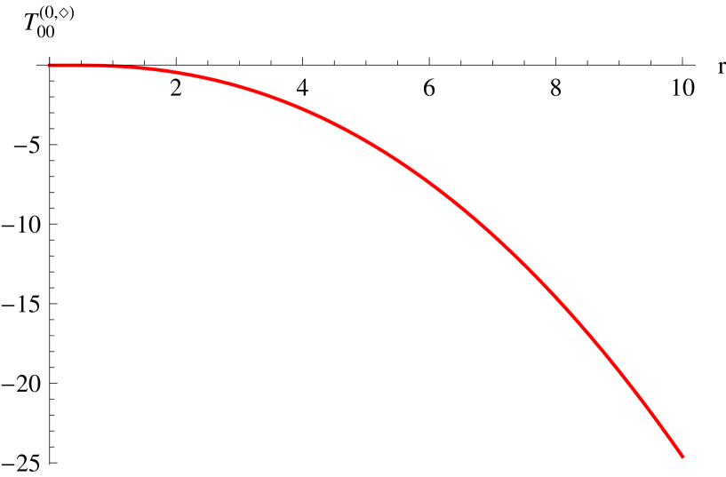
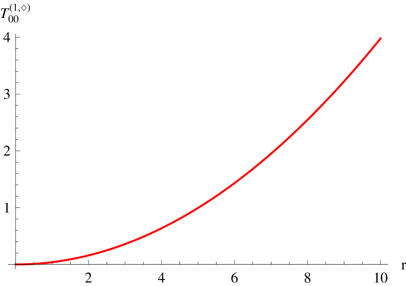
Figure 1: $d=1$: graphs of $T_{00}^{(0,\lozenge)}$ and $T_{00}^{(1,\lozenge)}$ .

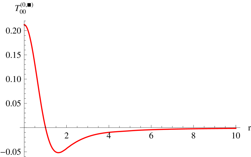
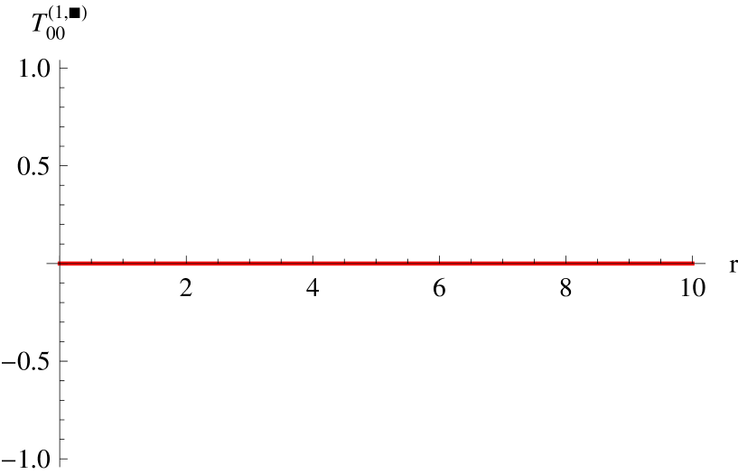
Figure 2: $d=1$: graphs of $T_{00}^{(0,\blacksquare)}$ and $T_{00}^{(1,\blacksquare)}$ .

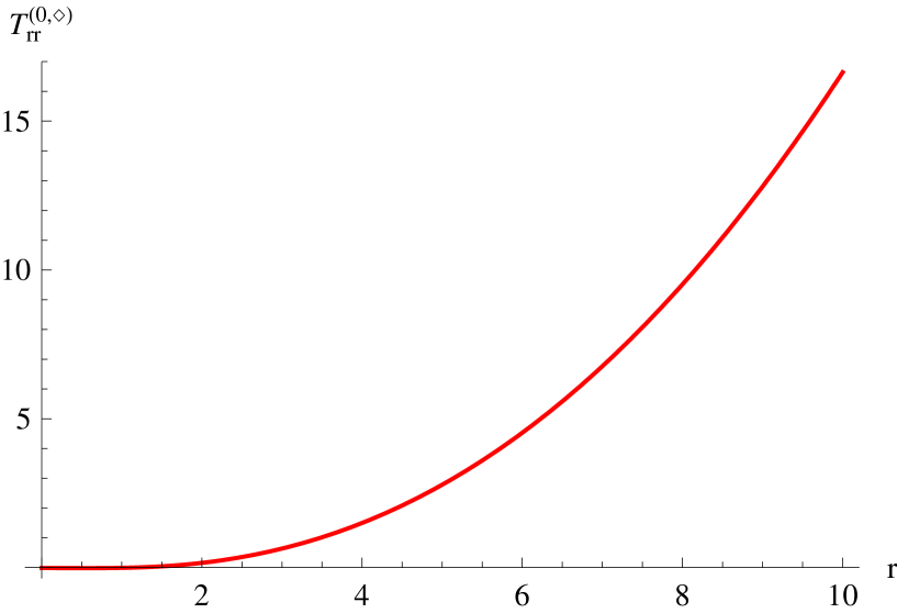
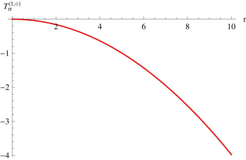
Figure 3: $d=1$: graphs of $T_{rr}^{(0,\lozenge)}$ and $T_{rr}^{(1,\lozenge)}$ .

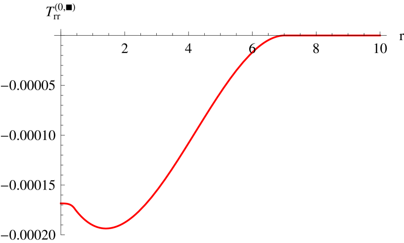
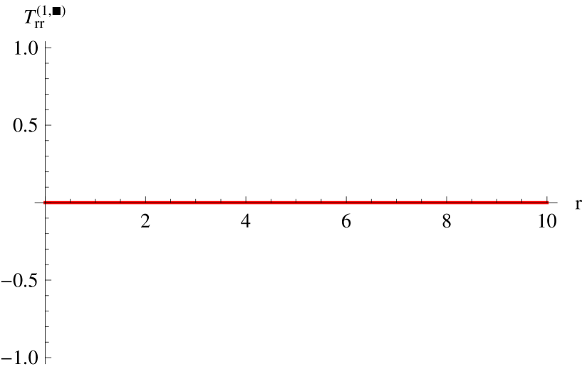
Figure 4: $d=1$: graphs of $T_{rr}^{(0,\blacksquare)}$ and $T_{rr}^{(1,\blacksquare)}$ .

Let us pass to evaluate the small and large $r$ asymptotics of the functions in Eq. (4.10). On the one hand, using Eq.s (3.32-3.35) (with $N=3$) we obtain, for $r=k|x^{1}|\to 0^{+}$,

$$\begin{split}T_{00}^{(0,\lozenge)}(r)&=-0.0153+0.0164\,r^{2}-0.0796\,r^{4}+0.0262\,r^{6}+O(r^{8})~{},\\ T_{00}^{(1,\lozenge)}(r)&=0.0398\,r^{2}+O(r^{8})~{},\\ T_{00}^{(0,\blacksquare)}(r)&=0.2121-0.3766\,r^{2}+0.2356\,r^{4}-0.0903\,r^{6}+O(r^{8})~{},\\ T_{00}^{(1,\blacksquare)}(r)&=O(r^{8})~{};\end{split}$$ (4.11)

$$\begin{split}T_{rr}^{(0,\lozenge)}(r)&=-0.0153-0.0164\,r^{2}+0.0265\,r^{4}-0.0052\,r^{6}+O(r^{8})~{},\\ T_{rr}^{(1,\lozenge)}(r)&=-0.0398\,r^{2}+O(r^{8})~{},\\ T_{rr}^{(0,\blacksquare)}(r)&=-0.0002-0.0001\,r^{4}+O(r^{8})~{},\\ T_{rr}^{(1,\blacksquare)}(r)&=O(r^{8})~{}.\end{split}$$ (4.12)

The numerical coefficients appearing here and in other small $r$ expansions are obtained from numerical computation of the integrals in (3.35).

On the other hand, using Eq.s (3.39) (3.45) (3.46) (with $K=3$, $\lambda=0$) we obtain the following asymptotic expansions, for $r=k|x^{1}|\to+\infty$:

$$\begin{split}T_{00}^{(0,\lozenge)}(r)&=-{r^{2}\over 8\pi}\Big{(}\ln{r^{2}}+\gamma_{EM}+1\Big{)}+{1\over 8\pi\,r^{2}}+{49\over 120\pi\,r^{6}}+O(r^{-8}\ln r^{2})~{},\\ T_{00}^{(1,\lozenge)}(r)&={r^{2}\over 8\pi}+O(r^{-8}\ln r^{2})~{},\\ T_{00}^{(0,\blacksquare)}(r)&=-{1\over 2\pi\,r^{2}}-{5\over 3\pi\,r^{6}}+O(r^{-8}\ln r^{2})~{},\\ T_{00}^{(1,\blacksquare)}(r)&=O(r^{-8}\ln r^{2})~{};\end{split}$$ (4.13)

$$\begin{split}T_{rr}^{(0,\lozenge)}(r)&={r^{2}\over 8\pi}\Big{(}\ln{r^{2}}+\gamma_{EM}-1\Big{)}+{1\over 24\pi\,r^{2}}+{7\over 120\pi\,r^{6}}+O(r^{-8}\ln r^{2})~{},\\ T_{rr}^{(1,\lozenge)}(r)&=-{r^{2}\over 8\pi}+O(r^{-8}\ln r^{2})~{},\\ T_{rr}^{(0,\blacksquare)}(r)&=O(r^{-8}\ln r^{2})~{},\\ T_{rr}^{(1,\blacksquare)}(r)&=O(r^{-8}\ln r^{2})~{}.\end{split}$$ (4.14)

Let us now discuss the bulk energy; using the expression (3.55) with $n=2$ and evaluating numerically the integral appearing therein, we infer

$$E^{ren}=(0.0430546469\pm 10^{-10})\,k~{}.$$ (4.15)

4.2   Case $d=2$.

Consider the general framework of subsection 3.5; in this case we use the (rescaled) polar coordinates ${\bf q}=(r,\theta_{1})\in(0,+\infty)\times[0,2\pi)$, fulfilling (see Eq. (3.11)) ()

$$k\,x^{1}=r\cos\theta_{1}~{},\qquad k\,x^{2}\!=r\sin\theta_{1}~{}.$$ (4.16)

Proceeding as in the one dimensional case, with some effort we obtain the following integral representation for the zeta-regularized stress-energy VEV (compare with Eq. (3.18) and recall that dependence on $\xi$ is understood):

$$\langle 0|\widehat{T}^{u}_{\mu\nu}({\bf q})|0\rangle={k^{3}\over\Gamma({u+1\over 2})}\left({\kappa\over k}\right)^{\!\!u}\!\int_{0}^{+\infty}\!\!\!d\tau\;\tau^{-{5\over 2}+{u\over 2}}\,{\mathcal{H}}^{(u)}_{\mu\nu}(\tau\,;{\bf q})\;\quad(\mu,\nu\in\{0,r,\theta_{1}\})~{},$$ (4.17)

where the tensor ${\mathcal{H}}^{(u)}_{\mu\nu}$ is diagonal and, concerning the diagonal components, we have

$$\begin{split}&\hskip 147.95424pt{\mathcal{H}}^{(u)}_{00}(\tau\,;{\bf q}):=\\ &A_{2}(\tau,r)\!\left[-(1\!-\!u)(1\!+\!4\xi)+(1\!-\!4\xi)\!\left({2\tau\over\sinh{2\tau}}\right)\!\left(2+r^{2}\,{\sinh{4\tau}\over 2\cosh^{2}\!\tau}\right)\!\right]\,,\end{split}$$ (4.18)

$${\mathcal{H}}^{(u)}_{rr}(\tau\,;{\bf q}):=A_{2}(\tau,r)\!\left[8\xi\,{\tau\over\tanh\tau}-(1\!-\!4\xi)\!\left(1\!-\!u+r^{2}\,{2\tau\over\cosh^{2}\!\tau}\right)\!\right]\,,$$ (4.19)

$${\mathcal{H}}^{(u)}_{\theta_{1}\theta_{1}}(\tau\,;{\bf q}):=\left({r\over k}\right)^{\!\!2}A_{2}(\tau,r)\!\left[8\xi\,{\tau\over\tanh\tau}-(1\!-\!4\xi)\!\left(\!1\!-\!u+r^{2}\,{2\tau\,\cosh{2\tau}\over\cosh^{2}\!\tau}\right)\!\right]\!.$$ (4.20)

In the above, for simplicity of notation we have put

$$A_{2}(\tau,r):={1\over 64\,\pi}\;e^{-r^{2}\tanh\tau}\left({2\tau\over\sinh{2\tau}}\right)\,.$$ (4.21)

Again, the features indicated by Eq.s (3.22) (3.23) (and related comments) are all possessed by the expressions (4.18-4.21) for ${\mathcal{H}}^{(u)}_{\mu\nu}$. So, we can analytically continue in $u$ the expression in Eq. (4.17) integrating by parts $n$ times, with $n>3/2$ (see Eq.s (3.24) (3.26)); we choose

$$n=2~{},$$ (4.22)

giving

$$\langle 0|\widehat{T}^{u}_{\mu\nu}({\bf q})|0\rangle={k^{3}\over\Gamma({u+1\over 2})}\,{1\over({u\over 2}\!-\!{3\over 2})({u\over 2}\!-\!{1\over 2})}\left({\kappa\over k}\right)^{\!\!u}\!\int_{0}^{+\infty}\!\!\!\!d\tau\;\tau^{{u\over 2}-{1\over 2}}\,\partial_{\tau}^{2}{\mathcal{H}}^{(u)}_{\mu\nu}(\tau;{\bf q})~{}.$$ (4.23)

Patently, each component of $\langle 0|\widehat{T}^{u}_{\mu\nu}|0\rangle$ is regular at $u=0$; thus, we can obtain the renormalized version of the stress-energy VEV by simply putting $u=0$ in Eq. (4.23) (we already noticed this property in general for the cases with even spatial dimension $d$; see below Eq. (3.26)). In conclusion,

$$\langle 0|\widehat{T}_{\mu\nu}({\bf q})|0\rangle_{ren}=k^{3}\,T^{(0)}_{\mu\nu}(r)~{},$$ (4.24)

$$T^{(0)}_{\mu\nu}(r):=\int_{0}^{+\infty}\!\!\!d\tau\;e^{-r^{2}\tanh\tau}\,{\mathcal{P}}^{(0)}_{\mu\nu}(\tau\,;r)~{},\quad\!{\mathcal{P}}^{(0)}_{\mu\nu}(\tau;r):={4\over 3\sqrt{\pi\,\tau}}\;e^{r^{2}\tanh\tau}\;\partial_{\tau}^{2}{\mathcal{H}}^{(0)}_{\mu\nu}(\tau;{\bf q})$$

(compare with Eq.s (3.28-3.30)); also in this case, we easily check that ${\mathcal{P}}^{(0)}_{\mu\nu}$ is a polynomial of degree $N=3$ in $r^{2}$. Next, we proceed as we did in the previous subsection for the case of spatial dimension $d=1$: we evaluate numerically the integrals in Eq. (4.24) and separate the conformal and non-conformal parts $\lozenge,\blacksquare$ of each component (see Eq. (3.31)), noting that Eq. (2.14) gives

$$\xi_{2}={1\over 8}~{}.$$ (4.25)

The forthcoming Fig.s 5-7 show the graphs of the functions

$$r\mapsto T_{\mu\nu}^{(0,\times)}(r)\;(\mu\!=\!\nu\!\in\!\{0,r\})\,,~{}(k/r)^{2}\,T_{\theta_{1}\theta_{1}}^{(0,\times)}(r)\qquad\mbox{for $\times\in\{\lozenge,\blacksquare\}$}~{}.$$ (4.26)

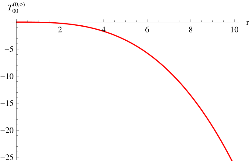
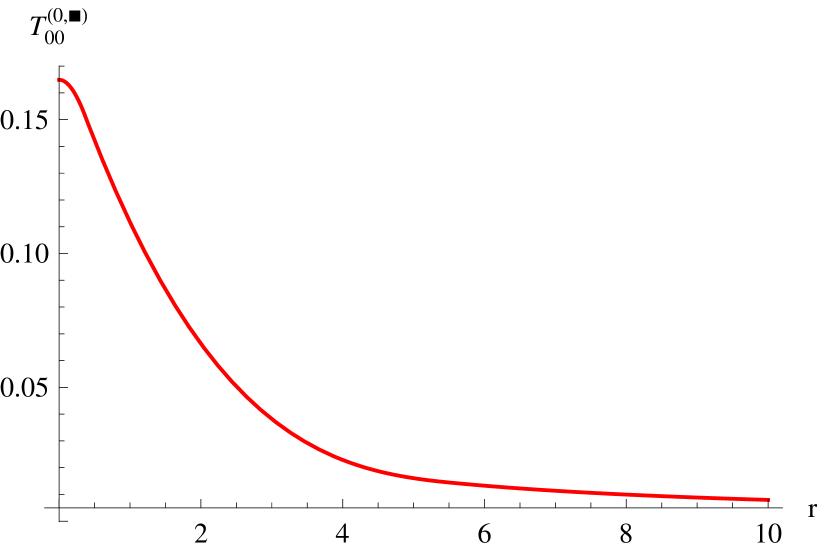
Figure 5: $d=2$: graphs of $T_{00}^{(0,\lozenge)}$ and $T_{00}^{(0,\blacksquare)}$ .

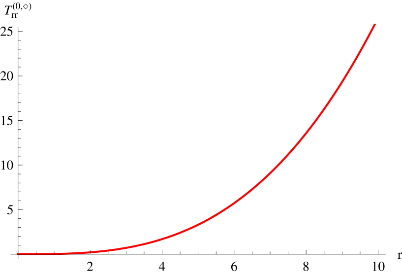
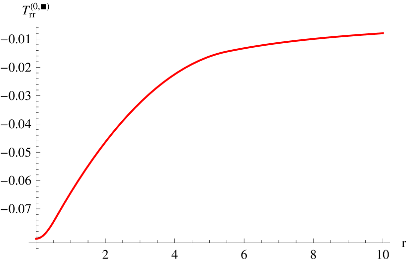
Figure 6: $d=2$: graphs of $T_{rr}^{(0,\lozenge)}$ and $T_{rr}^{(0,\blacksquare)}$ .

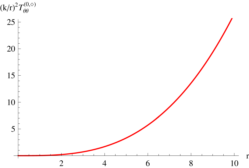
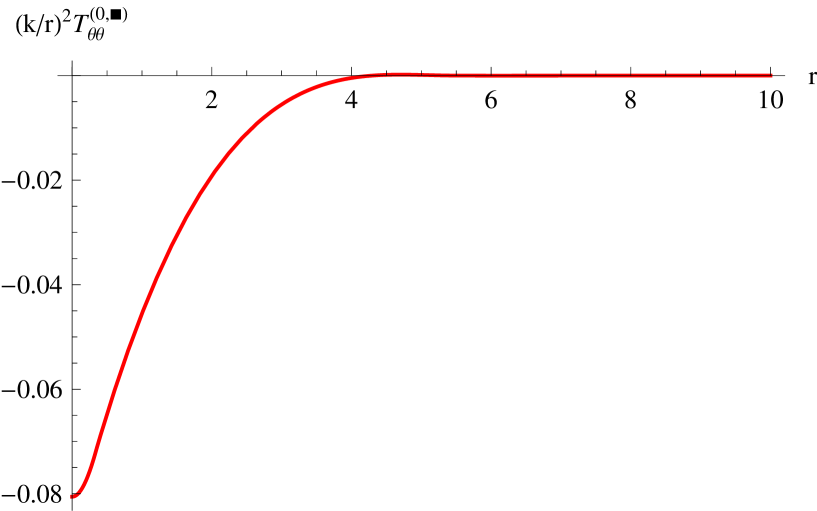
Figure 7: $d=2$: graphs of $(k/r)^{2}T_{\theta_{1}\theta_{1}}^{(0,\lozenge)}$ and $(k/r)^{2}T_{\theta_{1}\theta_{1}}^{(0,\blacksquare)}$ .

Now, let us consider the small and large $r$ asymptotics of the functions in (4.26). On the one hand, Eq.s (3.32-3.35) (with $N=3$) give, for $r=k|{\bf x}|\to 0^{+}$,

$$\begin{split}T_{00}^{(0,\lozenge)}(r)&=-0.0017-0.0134\,r^{2}-0.0154\,r^{4}+0.0027\,r^{6}+O(r^{8})~{},\\ T_{00}^{(0,\blacksquare)}(r)&=0.1649-0.1069\,r^{2}+0.0516\,r^{4}-0.0141\,r^{6}+O(r^{8})~{};\end{split}$$ (4.27)

$$\begin{split}T_{rr}^{(0,\lozenge)}(r)&=-0.0010+0.0207\,r^{2}+0.0114\,r^{4}-0.0013\,r^{6}+O(r^{8})~{},\\ T_{rr}^{(0,\blacksquare)}(r)&=-0.0806+0.0267\,r^{2}-0.0133\,r^{4}+0.0018\,r^{6}+O(r^{8})~{};\\ \end{split}$$ (4.28)

$$\begin{split}(k/r)^{2}\,T_{\theta_{1}\theta_{1}}^{(0,\lozenge)}(r)&=-0.0010+0.0140\,r^{2}+0.0153\,r^{4}-0.0027\,r^{6}+O(r^{8})~{},\\ (k/r)^{2}\,T_{\theta_{1}\theta_{1}}^{(0,\blacksquare)}(r)&=-0.0806+0.0802\,r^{2}-0.0440\,r^{4}+0.0124\,r^{6}+O(r^{8})~{}.\\ \end{split}$$ (4.29)

Again, the above coefficients were obtained calculating numerically the integrals in Eq. (3.35).

On the other hand, using Eq.s (3.39) (3.45) (3.46) (with $K=5$, $\lambda=-1/2$; note that no logarithmic term $\ln r^{2}$ appears in this case) we obtain the following asymptotic expansions for $r=k|{\bf x}|\to+\infty$:

$$\begin{split}T_{00}^{(0,\lozenge)}(r)&=-{r^{3}\over 12\pi}-{19\over 2560\pi\,r^{5}}+O(r^{-9})~{},\\ T_{00}^{(0,\blacksquare)}(r)&={1\over 4\pi\,r}+{3\over 32\pi\,r^{5}}+O(r^{-9})~{};\end{split}$$ (4.30)

$$\begin{split}T_{rr}^{(0,\lozenge)}(r)&={r^{3}\over 12\pi}+{1\over 48\pi\,r}-{17\over 2560\pi\,r^{5}}+O(r^{-9})~{},\\ T_{rr}^{(0,\blacksquare)}(r)&=-{1\over 4\pi\,r}+{1\over 32\pi\,r^{5}}+O(r^{-9})~{};\end{split}$$ (4.31)

$$\begin{split}(k/r)^{2}\,T_{\theta_{1}\theta_{1}}^{(0,\lozenge)}(r)&={r^{3}\over 12\pi}-{1\over 96\pi\,r}++{33\over 2560\pi\,r^{5}}+O(r^{-9})~{},\\ (k/r)^{2}\,T_{\theta_{1}\theta_{1}}^{(0,\blacksquare)}(r)&=-{1\over 8\pi\,r^{5}}+O(r^{-9})~{}.\end{split}$$ (4.32)

As for the bulk energy, using again the expression (3.55) with $n=3$ and evaluating numerically the integral appearing therein, we obtain

$$E^{ren}=-(0.0180207591\pm 10^{-10})\,k~{}.$$ (4.33)

4.3   Case $d=3$.

In this case we use the coordinates ${\bf q}=(r,\theta_{1},\theta_{2})\in(0,+\infty)\times(0,\pi)\times[0,2\pi)$, which are related to the Cartesian coordinates ${\bf x}\equiv(x_{1},x_{2},x_{3})$ via (see Eq. (3.11)) ()

$$k\,x^{1}=r\cos\theta_{1}~{},\quad k\,x^{2}=r\sin\theta_{1}\cos\theta_{2}~{},\quad k\,x^{3}=r\sin\theta_{1}\sin\theta_{2}~{}.$$ (4.34)

Similarly to what we did in the previous two subsections, after lenghty computations, we can express the zeta-regularized stress-energy VEV as (compare with Eq. (3.18) and recall that dependence on $\xi$ is understood)

$$\langle 0|\widehat{T}^{u}_{\mu\nu}({\bf q})|0\rangle={k^{4}\over\Gamma({u+1\over 2})}\left({\kappa\over k}\right)^{\!\!u}\!\int_{0}^{+\infty}\!\!\!\!d\tau\;\tau^{-3+{u\over 2}}\,{\mathcal{H}}^{(u)}_{\mu\nu}(\tau\,;{\bf q})\quad(\mu,\nu\!\in\!\{0,r,\theta_{1},\theta_{2}\})\,,\!$$ (4.35)

where ${\mathcal{H}}^{(u)}_{\mu\nu}$ is diagonal and we only have to consider the independent components

$$\begin{split}&\hskip 147.95424pt{\mathcal{H}}^{(u)}_{00}(\tau\,;{\bf q}):=\\ &A_{3}(\tau,r)\!\left[-(1\!-\!u)(1\!+\!4\xi)+(1\!-\!4\xi)\!\left(\!{2\tau\over\sinh{2\tau}}\!\right)\!\!\left(3+r^{2}\,{\sinh{3\tau}-\sinh{\tau}\over\cosh{\tau}}\right)\right]\,,\end{split}$$ (4.36)

$$\begin{split}&\hskip 147.95424pt{\mathcal{H}}^{(u)}_{rr}(\tau\,;{\bf q}):=\\ &A_{3}(\tau,r)\!\left[8\xi\,{\tau\over\tanh\tau}-(1\!-\!4\xi)\!\left(1\!-\!u+\!\left(\!{2\tau\over\sinh{2\tau}}\!\right)\!\Big{(}1\!+\!2r^{2}\tanh\tau\Big{)}\!\right)\right]\,,\end{split}$$ (4.37)

$$\begin{split}&\hskip 147.95424pt{\mathcal{H}}^{(u)}_{\theta_{1}\theta_{1}}(\tau\,;{\bf q}):=\\ &\left({r\over k}\right)^{\!\!2}A_{3}(\tau,r)\!\left[8\xi\,{\tau\over\tanh\tau}-(1\!-\!4\xi)\!\left(1\!-\!u+\!\left(\!{2\tau\over\sinh{2\tau}}\!\right)\!\Big{(}1\!+\!{r^{2}\over\cosh^{2}\!{2\tau}}\Big{)}\!\right)\right]\end{split}$$ (4.38)

(for the remaining diagonal component, i.e. ${\mathcal{H}}^{(u)}_{\theta_{2}\theta_{2}}(\tau\,;{\bf q})$, see Eq. (3.22)). In the above, for simplicity of notation we have put

$$A_{3}(\tau,r):={1\over 64\,\pi^{3/2}}\;e^{-r^{2}\tanh\tau}\left({2\tau\over\sinh{2\tau}}\right)^{\!\!3/2}\,.$$ (4.39)

Also this time, the expressions (4.36-4.39) for ${\mathcal{H}}^{(u)}_{\mu\nu}$ possess the properties indicated in Eq.s (3.22) (3.23) (and in the related comments); thus, we can obtain the analytic continuation in $u$ of the expression in Eq. (4.35) integrating by parts $n$ times, for any $n>2$ (see Eq. (3.26)). For definiteness, we fix

$$n=3~{},$$ (4.40)

so that Eq. (3.24) reads

$$\langle 0|\widehat{T}^{u}_{\mu\nu}({\bf q})|0\rangle=-{k^{4}\over\Gamma({u+1\over 2})}\,{1\over({u\over 2}\!-\!2)({u\over 2}\!-\!1){u\over 2}}\left({\kappa\over k}\right)^{\!\!u}\!\int_{0}^{+\infty}\!\!d\tau\;\tau^{u\over 2}\,\partial_{\tau}^{3}{\mathcal{H}}^{(u)}_{\mu\nu}(\tau;{\bf q})\,.\!$$ (4.41)

As in all cases with odd spatial dimension, the analytic continuation of the regularized stress-energy VEV given in Eq. (4.41) has a simple pole in $u=0$ (recall subsection 3.5). In consequence of this, we have to adopt the extended version of the zeta approach to define the renormalized VEV $\langle 0|\widehat{T}_{\mu\nu}({\bf q})|0\rangle_{ren}$, taking the regular part in $u=0$ of Eq. (4.41) (see Eq. (3.27)); with some effort, we obtain

$$\langle 0|\widehat{T}_{\mu\nu}({\bf q})|0\rangle_{ren}=k^{4}\Big{(}T^{(0)}_{\mu\nu}(r)+M_{\kappa,k}\,T^{(1)}_{\mu\nu}(r)\Big{)}~{},$$ (4.42)

$$\begin{split}&\hskip 27.03003ptT^{(0)}_{\mu\nu}(r):=\int_{0}^{+\infty}\!\!\!d\tau\;e^{-r^{2}\tanh\tau}\Big{[}{\mathcal{P}}^{(0)}_{\mu\nu}(\tau\,;r)+\ln\tau\;{\mathcal{P}}^{(1)}_{\mu\nu}(\tau\,;r)\Big{]}~{},\\ &T^{(1)}_{\mu\nu}(r):=\int_{0}^{+\infty}\!\!\!d\tau\;e^{-r^{2}\tanh\tau}\;{\mathcal{P}}^{(1)}_{\mu\nu}(\tau\,;r)~{},\qquad M_{\kappa,k}:=\gamma_{EM}\!+\!2\ln\!\left(\!{2\mu\over k}\right),\end{split}$$

where

$$\begin{split}&{\mathcal{P}}^{(0)}_{\mu\nu}(\tau\,;r):=-\,{1\over 4\sqrt{\pi}}\;e^{r^{2}\tanh\tau}\;\Big{[}3\,\partial_{\tau}^{3}{\mathcal{H}}^{(0)}_{\mu\nu}(\tau;{\bf q})+4\,\partial_{u}\Big{|}_{u=0}\partial_{\tau}^{3}{\mathcal{H}}^{(u)}_{\mu\nu}(\tau;{\bf q})\Big{]}~{},\\ &\hskip 56.9055pt{\mathcal{P}}^{(1)}_{\mu\nu}(\tau\,;r):=-{1\over 2\sqrt{\pi}}\;e^{r^{2}\tanh\tau}\;\partial_{\tau}^{3}{\mathcal{H}}^{(0)}_{\mu\nu}(\tau;{\bf q})~{};\end{split}$$ (4.43)

this time, we readily infer that ${\mathcal{P}}^{(0)}_{\mu\nu}$, ${\mathcal{P}}^{(1)}_{\mu\nu}$ are polynomials of degree $N=4$ in $r^{2}$. Now, we evaluate numerically the integrals in Eq. (4.42) and distinguish between the conformal and non-conformal parts $\lozenge$, $\blacksquare$ of each component; once more we refer to Eq. (3.31), recalling that for $d=3$ we have (see Eq. (2.14))

$$\xi_{3}={1\over 6}~{}.$$ (4.44)

The forthcoming Fig.s 8-13 show the graphs of the functions

$$r\mapsto T_{00}^{(a,\times)}(r)\,,\;T_{rr}^{(a,\times)}(r)\,,\;(k/r)^{2}\,T_{\theta_{1}\theta_{1}}^{(a,\times)}(r)\quad\;\mbox{for $a\!\in\!\{0,1\}$, $\times\!\in\!\{\lozenge,\blacksquare\}$}~{}.$$ (4.45)

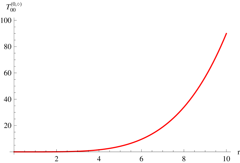
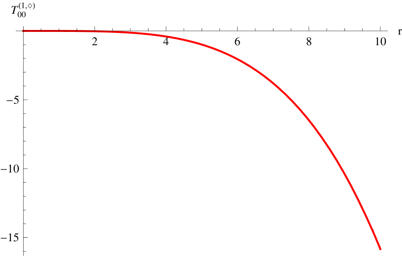
Figure 8: $d=3$: graphs of $T_{00}^{(0,\lozenge)}$ and $T_{00}^{(1,\lozenge)}$ .

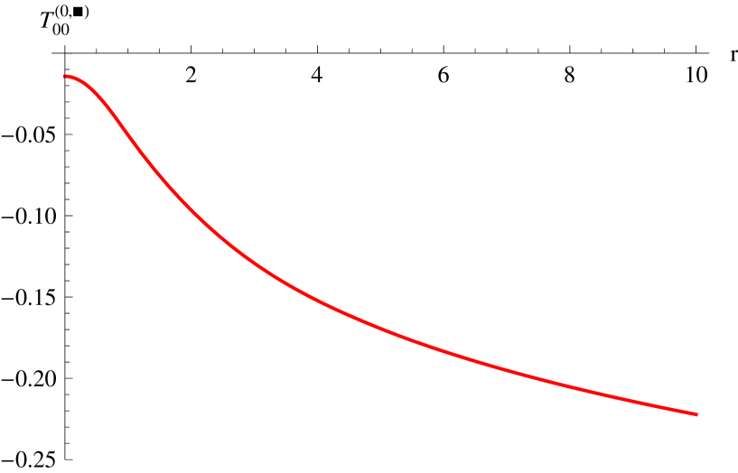
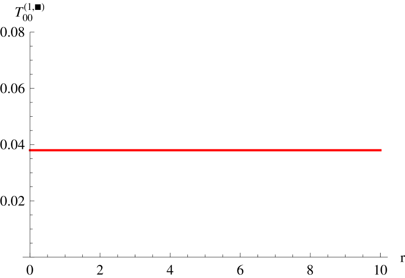
Figure 9: $d=3$: graphs of $T_{00}^{(0,\blacksquare)}$ and $T_{00}^{(1,\blacksquare)}$ .

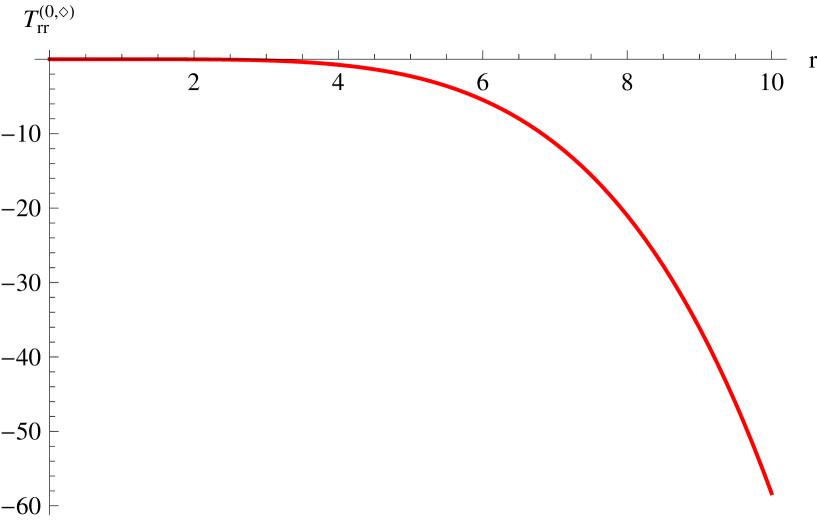
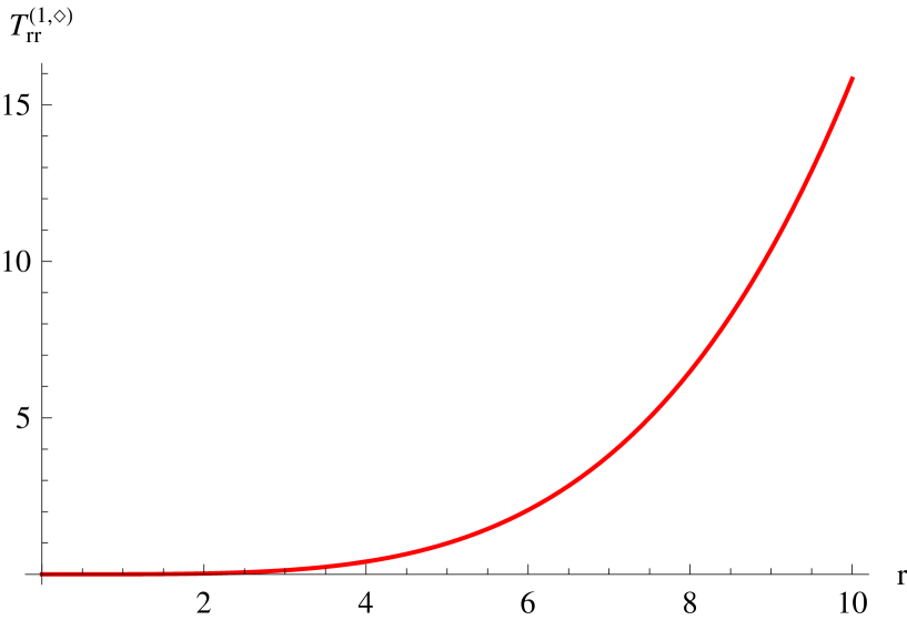
Figure 10: $d=3$: graphs of $T_{rr}^{(0,\lozenge)}$ and $T_{rr}^{(1,\lozenge)}$ .

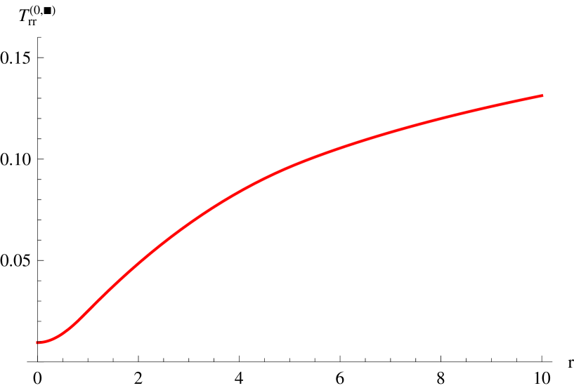
Figure 11: $d=3$: graphs of $T_{rr}^{(0,\blacksquare)}$ and $T_{rr}^{(1,\blacksquare)}$ .

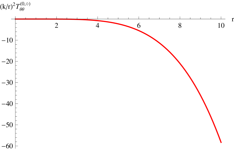
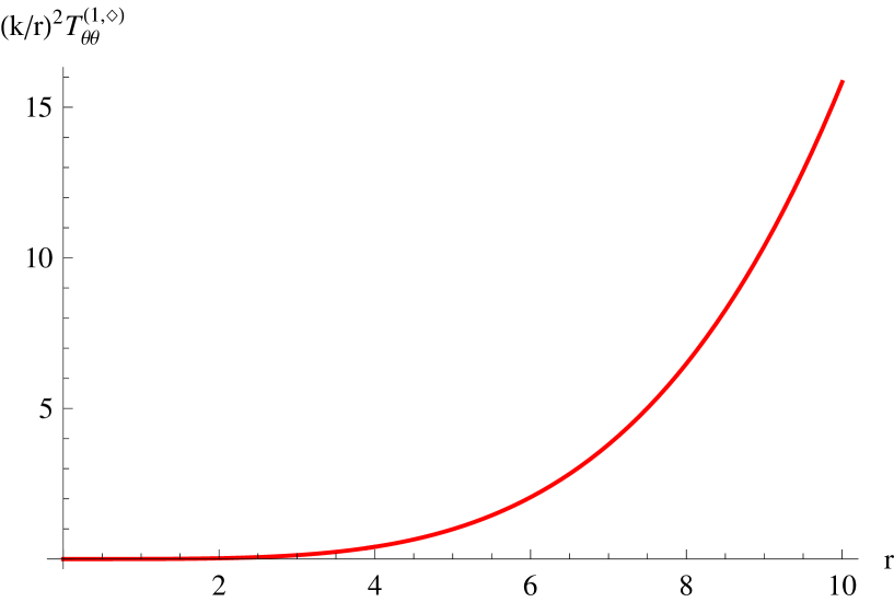
Figure 12: $d=3$: graphs of $(k/r)^{2}T_{\theta_{1}\theta_{1}}^{(0,\lozenge)}$ and $(k/r)^{2}T_{\theta_{1}\theta_{1}}^{(1,\lozenge)}$ .

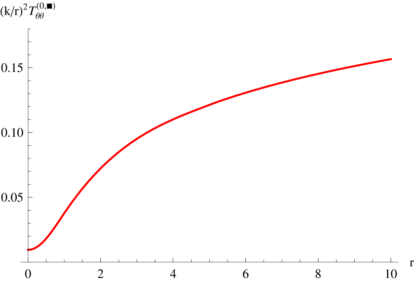
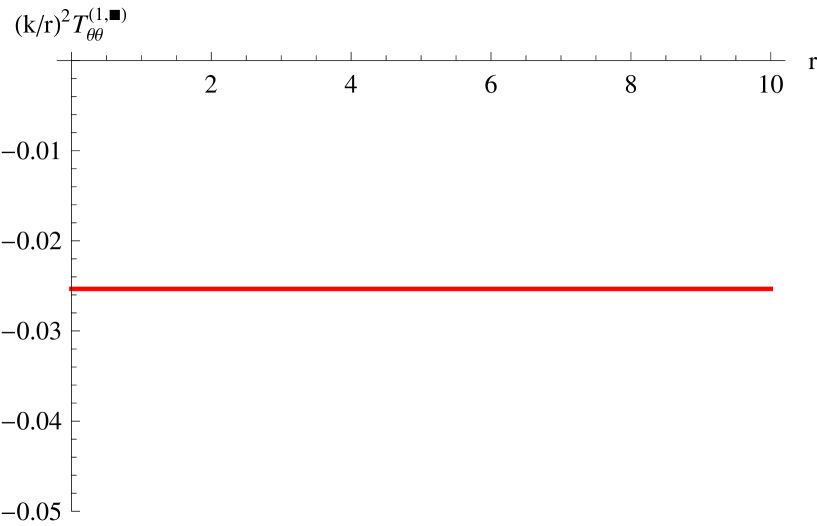
Figure 13: $d=3$: graphs of $(k/r)^{2}T_{\theta_{1}\theta_{1}}^{(0,\blacksquare)}$ and $(k/r)^{2}T_{\theta_{1}\theta_{1}}^{(1,\blacksquare)}$ .

In conclusion, let us discuss the small and large $r$ asymptotics of the functions in (4.45). On the one hand, Eq.s (3.32-3.35) (with $N=4$) yield, for $r=k|{\bf x}|\to 0^{+}$,

$$\begin{split}T_{00}^{(0,\lozenge)}(r)\!&=-0.0047-0.0024\,r^{2}\!+0.0028\,r^{4}\!+0.0006\,r^{6}\!-0.0001\,r^{8}\!+\!O(r^{10})\,,\!\\ T_{00}^{(1,\lozenge)}(r)\!&=-0.0016\,r^{4}\!+O(r^{10})~{},\\ T_{00}^{(0,\blacksquare)}(r)\!&=-0.0143-0.0468\,r^{2}\!+0.0134\,r^{4}\!-0.0033\,r^{6}\!+0.0007\,r^{8}\!+\!O(r^{10})\,,\!\\ T_{00}^{(1,\blacksquare)}(r)\!&=0.0380+O(r^{10})~{};\end{split}$$ (4.46)

$$\begin{split}T_{rr}^{(0,\lozenge)}(r)&=-0.0016+0.0039\,r^{2}\!-0.0003\,r^{4}\!-0.0005\,r^{6}\!+O(r^{10})~{},\\ T_{rr}^{(1,\lozenge)}(r)&=0.0016\,r^{4}+O(r^{10})~{},\\ T_{rr}^{(0,\blacksquare)}(r)&=0.0095+0.0188\,r^{2}\!-0.0038\,r^{4}\!+0.0007\,r^{6}\!-0.0001\,r^{8}\!+O(r^{10})\,,\\ T_{rr}^{(1,\blacksquare)}(r)&=-0.0253+O(r^{10})~{};\end{split}$$ (4.47)

$$\begin{split}(k/r)^{2}\,T_{\theta_{1}\theta_{1}}^{(0,\lozenge)}(r)&=-0.0016+0.0023\,r^{2}+0.0004\,r^{4}-0.0006\,r^{6}+0.0001\,r^{8}+O(r^{10})~{},\\ (k/r)^{2}\,T_{\theta_{1}\theta_{1}}^{(1,\lozenge)}(r)&=0.0016\,r^{4}+O(r^{10})~{},\\ (k/r)^{2}\,T_{\theta_{1}\theta_{1}}^{(0,\blacksquare)}(r)&=0.0095+0.0375\,r^{2}-0.0115\,r^{4}+0.0030\,r^{6}-0.0006\,r^{8}+O(r^{10})~{},\\ (k/r)^{2}\,T_{\theta_{1}\theta_{1}}^{(1,\blacksquare)}(r)&=-0.0253+O(r^{10})~{}.\end{split}$$ (4.48)

  
On the other hand, Eq.s (3.39) (3.45) (3.46) (with $K=4$, $\lambda=0$) allow us to infer the following asymptotic expansion, for $r=k|{\bf x}|\to+\infty$:

$$\begin{split}T_{00}^{(0,\lozenge)}(r)&={r^{4}\over 64\pi^{2}}\,\Big{(}\ln{r^{2}}\!+\gamma_{EM}\!+{1\over 2}\Big{)}-{5\over 96\pi^{2}}-{23\over 2880\pi^{2}r^{4}}+O(r^{-8}\ln r^{2})~{},\\ T_{00}^{(1,\lozenge)}(r)&=-{r^{4}\over 64\pi^{2}}+O(r^{-8}\ln r^{2})~{},\\ T_{00}^{(0,\blacksquare)}(r)&=-{3\over 8\pi^{2}}\,\Big{(}\ln{r^{2}\!+\!\gamma_{EM}\!+{2\over 3}}\Big{)}+{1\over 12\pi^{2}r^{4}}+O(r^{-8}\ln r^{2})~{},\\ T_{00}^{(1,\blacksquare)}(r)&={3\over 8\pi^{2}}+O(r^{-8}\ln r^{2})~{};\end{split}$$ (4.49)

$$\begin{split}T_{rr}^{(0,\lozenge)}(r)&=-{r^{4}\over 64\pi^{2}}\!\left(\ln{r^{2}}\!+\gamma_{EM}\!-{3\over 2}\right)\!+{1\over 96\pi^{2}}-{49\over 2880\pi^{2}r^{4}}+O(r^{-8}\ln r^{2})~{},\\ T_{rr}^{(1,\lozenge)}(r)&={r^{4}\over 64\pi^{2}}+O(r^{-8}\ln r^{2})~{},\\ T_{rr}^{(0,\blacksquare)}(r)&={1\over 4\pi^{2}}\,\Big{(}\ln{r^{2}}\!+\!\gamma_{EM}\Big{)}\!+{1\over 6\pi^{2}r^{4}}+O(r^{-8}\ln r^{2})~{},\\ T_{rr}^{(1,\blacksquare)}(r)&=-{1\over 4\pi^{2}}+O(r^{-8}\ln r^{2})~{};\end{split}$$ (4.50)

$$(k/r)^{2}\,T_{\theta_{1}\theta_{1}}^{(0,\lozenge)}(r)=-{r^{4}\over 64\pi^{2}}\left(\ln{r^{2}}\!+\gamma_{EM}\!-{3\over 2}\right)\!-{1\over 96\pi^{2}}+{31\over 2880\pi^{2}r^{4}}+O(r^{-8}\ln r^{2})~{},$$

$$\begin{split}(k/r)^{2}\,T_{\theta_{1}\theta_{1}}^{(1,\lozenge)}(r)&={r^{4}\over 64\pi^{2}}+O(r^{-8}\ln r^{2})~{},\\ (k/r)^{2}\,T_{\theta_{1}\theta_{1}}^{(0,\blacksquare)}(r)&={1\over 4\pi^{2}}\,\Big{(}\ln{r^{2}}\!+\!\gamma_{EM}\!+\!1\Big{)}-{1\over 6\pi^{2}r^{4}}+O(r^{-8}\ln r^{2})~{},\\ (k/r)^{2}\,T_{\theta_{1}\theta_{1}}^{(1,\blacksquare)}(r)&=-{1\over 4\pi^{2}}+O(r^{-8}\ln r^{2})~{}.\end{split}$$ (4.51)

Finally, Eq. (3.55) with $n=4$ and numerical evaluation of the corresponding integral allow us to derive the bulk energy

$$E^{ren}=-(0.0078607119\pm 10^{-10})\,k~{}.$$ (4.52)

This result agrees with the one obtained by Actor and Bender [2] using a different method ().

Acknowledgments. This work was partly supported by INdAM, INFN and by MIUR, PRIN 2010 Research Project “Geometric and analytic theory of Hamiltonian systems in finite and infinite dimensions”.

Appendix A Appendix. Asymptotic expansions for certain integrals

Hereafter we show how to obtain the expansions (3.34) (3.41), holding respectively for the functions defined via the integral representations (3.32) (3.39). The proofs are given in subsections A.1 and A.3; subsection A.2 is an interlude on gamma-type functions, useful in view of subsection A.3.

A.1   Derivation of Eq.s (3.34-3.37).

Let us consider the framework of subsection 3.6, where

$$F(r):=\int_{0}^{+\infty}\!\!\!d\tau\;e^{-r^{2}h(\tau)}\,P(\tau\,;r)~{},\quad\!P(\tau\,;r)=\sum_{i=0}^{N}p_{i}(\tau)\,r^{2i}\quad(r\in(0,+\infty))~{},$$ (A.1)

($h$ a positive bounded function, $p_{i}$ ($i\in\{0,...,N\}$) some integrable functions).

To evaluate $F(r)$ we start from Taylor’s formula with Lagrange remainder for the exponential; this ensures that, for any $z\in(0,+\infty)$ and any $M\in\{0,1,2,...\}$,

$$\begin{split}&\hskip 51.21504pte^{-z}=\sum_{m=0}^{M}{(-z)^{m}\!\over m!}+\rho_{M+1}(z_{\star})\,z^{M+1}~{},\\ &\rho_{M+1}(z_{\star}):={1\over(M\!+\!1)!}\left.{d^{M+1}\over dz^{M+1}}\,e^{-z}\right|_{z=z_{\star}}={(-1)^{M+1}\over(M\!+\!1)!}\;e^{-z_{\star}}~{},\end{split}$$ (A.2)

for some $z_{\star}=z_{*}(z)\in(0,z)$; in particular, we have

$$|\rho_{M+1}(z_{\star})|\leqslant{1\over(M\!+\!1)!}~{}.$$ (A.3)

Substituting expansion (A.2) with $z=r^{2}h(\tau)$ and $M=N\!-\!i$ into Eq. (A.1), we readily infer

$$\begin{split}&F(r)=\sum_{i=0}^{N}\left[\sum_{m=0}^{N-i}\left({(-1)^{m}\!\over m!}\int_{0}^{+\infty}\!\!d\tau\;p_{i}(\tau)\,(h(\tau))^{m}\right)\!r^{2(m+i)}\;+\right.\\ &\hskip 79.6678pt\left.+\left(\int_{0}^{+\infty}\!\!d\tau\;p_{i}(\tau)\,(h(\tau))^{N-i+1}\,\rho_{N-i+1}(z_{\star}(\tau,r))\right)\!r^{2(N+1)}\right]~{},\end{split}$$ (A.4)

with $z_{\star}(\tau,r)\in(0,r^{2}h(\tau))$. Introducing a new summation index $i$ such that $m=j-i$, and performing the exchange $i\leftrightarrow j$ (), the above relation yields

$$F(r)=\sum_{i=0}^{N}a_{i}\,r^{2i}+R_{N+1}(r)\qquad\mbox{for $r\in(0,+\infty)$}~{},$$ (A.5)

where the coefficients $a_{i}\in{\bf R}$ are defined as in Eq. (3.35), while the remainder term $R_{N+1}(r)$ is

$$R_{N+1}(r):=\left(\sum_{i=0}^{N}\int_{0}^{+\infty}\!\!d\tau\;p_{i}(\tau)\,(h(\tau))^{N-i+1}\,\rho_{N-i+1}(z_{\star}(\tau,r))\right)r^{2(N+1)}~{}.$$ (A.6)

Using the estimate (A.3), we readily infer the uniform bound, holding for all $r\in(0,+\infty)$,

$$|R_{N+1}(r)|\leqslant\left(\sum_{i=0}^{N}{1\over(N\!-\!i\!+\!1)!}\int_{0}^{+\infty}\!\!d\tau\;|p_{i}(\tau)|\,(h(\tau))^{N-i+1}\right)r^{2(N+1)}~{};$$ (A.7)

this proves Eq. (3.36), with the expression (3.37) for the constant $C_{N+1}$ therein.

A.2   The incomplete gamma functions and the integral $\mathfrak{g}(s,x)$; asymptotics and bounds.

Let us first consider the “lower” and “upper” incomplete gamma functions, respectively defined as

$$\gamma(s,z):=\int_{0}^{z}dw\;e^{-w}\,w^{s-1}\qquad\mbox{for all $s\in{\bf C}$ with $\Re s>0$, $z\in(0,+\infty)$}~{},$$ (A.8)

$$\Gamma(s,z):=\int_{z}^{+\infty}\!\!dw\;e^{-w}\,w^{s-1}\qquad\mbox{for all $s\in{\bf C}$, $z\in(0,+\infty)$}~{}.$$ (A.9)

Hereafter we report some well-known properties of these functions (see [20], Chapter 8), to be used in the following subsection. First of all, there holds

$$\gamma(s,z)+\Gamma(s,z)=\Gamma(s)\qquad(s\notin\{0,-1,-2,...\})~{},$$ (A.10)

where $\Gamma(~{})$ is the Euler gamma function. Concerning the lower incomplete gamma, there hold the relations

$$\begin{split}&\gamma(s\!+\!1,z)=s\,\gamma(s,z)-e^{-z}z^{s}~{},\quad\;\gamma(s,z)=\Gamma(s)+O(z^{-\infty})~{}~{}\mbox{for $z\to+\infty$}~{};\\ &\hskip 105.2751pt0\leqslant\gamma(s,z)\leqslant\Gamma(s)\quad\mbox{for $s\in(0,+\infty)$}~{}.\end{split}$$ (A.11)

On the other hand, the upper incomplete gamma fulfills

$$\begin{split}&\Gamma(s\!+\!1,z)=s\,\Gamma(s,z)+e^{-z}z^{s}~{},\qquad\Gamma(s,z)=O(z^{-\infty})~{}~{}\mbox{for $z\to+\infty$}~{};\\ &\hskip 93.89418pt0\leqslant\Gamma(s,z)\leqslant\Gamma(z)\quad\mbox{for $s\in(0,+\infty)$}~{}.\end{split}$$ (A.12)

(both here and in Eq. (A.11), the remainder $O(z^{-\infty})$ indicates a quantity which is $O(z^{-N})$ for all $N\in\{0,1,2,...\}$). Let us move on to discuss the properties of the function $\mathfrak{g}(s,x)$ defined via the integral representation (see Eq. (3.43))

$$\mathfrak{g}(s,z):=\int_{0}^{z}\!dw\;e^{-w}w^{s-1}\ln w\qquad\!\mbox{for all $s\in{\bf C}$ with $\Re s>0$, $z\in(0,+\infty)$}\,.$$

First of all, since $\partial_{s}(w^{s-1})=w^{s-1}\ln w$, from the above definition and Eq. (A.8) it trivially follows that

$$\mathfrak{g}(s,z)=\partial_{s}\,\gamma(s,z)~{};$$ (A.13)

thus, using the recursive relation in Eq. (A.11), we can easily infer

$$\mathfrak{g}(s\!+\!1,z)=s\,\mathfrak{g}(s,z)+\gamma(s,z)-e^{-z}\,z^{s}\,\ln z\qquad(\Re s>0)~{}.$$ (A.14)

Now, let us show that

$$\mathfrak{g}(1,z)=-e^{-z}\ln z-\gamma_{EM}-\Gamma(0,z)$$ (A.15)

($\gamma_{EM}$ denotes the Euler-Mascheroni constant). To this purpose, let us write

$$\mathfrak{g}(1,z)=\lim_{\delta\to 0^{+}}\mathfrak{g}_{\delta}(1,z)~{},\qquad\mathfrak{g}_{\delta}(1,z):=\int_{\delta}^{z}\!dw\;e^{-w}\ln w\quad(\delta>0)~{}.$$ (A.16)

Consider the regularized function $\mathfrak{g}_{\delta}(1,z)$ and integrate by parts to obtain

$$\mathfrak{g}_{\delta}(1,z)=-e^{-x}\ln x+e^{-\delta}\ln\delta+\int_{\delta}^{z}\!dw\,e^{-w}w^{-1}~{};$$ (A.17)

now, note that (for $0<\delta<z$)

$$\int_{\delta}^{z}\!dw\,e^{-w}w^{-1}=\int_{\delta}^{+\infty}\!\!\!dw\,e^{-w}w^{-1}-\int_{z}^{+\infty}\!\!\!dw\,e^{-w}w^{-1}=\Gamma(0,\delta)-\Gamma(0,z)~{}.$$ (A.18)

Since $\Gamma(0,\delta)=-\ln\delta-\gamma_{EM}+O(\delta)$ for $\delta\to 0^{+}$ (see [20], p.177, Eq. 8.4.15), we have

$$\mathfrak{g}_{\delta}(1,z)=-e^{-x}\ln x-\gamma_{EM}-\Gamma(0,z)-(1-e^{-\delta})\ln\delta+O(\delta)\quad\,\mbox{for $\delta\to 0^{+}$},$$ (A.19)

which, along with Eq. (A.16), yields Eq. (A.15).

Let us proceed to prove that there holds the bound

$$\mathfrak{g}(s,z)\geqslant-s^{-2}\qquad\mbox{for all $s,z\in(0,+\infty)$}~{};$$ (A.20)

we are going to give the proof for $z<1$ and $z\geqslant 1$ separately. On the one hand, for $z<1$ (and $s>0$), there holds the following chain of inequalities:

$$\mathfrak{g}(s,z)\geqslant\int_{0}^{1}dw\;e^{-w}\,w^{s-1}\ln w\geqslant\int_{0}^{1}dw\;w^{s-1}\ln w=-s^{-2}~{},$$ (A.21)

where the first passage follows from the negativity of the integrand ($\ln w<0$, for $w\in(0,1)$), while for the second we used $e^{-w}\leqslant 1$ for $w\in(0,1)$. On the other hand, for $z>1$ (and $s>0$), we have

$$\begin{split}\mathfrak{g}(s,z)=\!\int_{0}^{1}\!dw\,e^{-w}w^{s-1}\ln w+\!\int_{1}^{z}\!dw\,e^{-w}w^{s-1}\ln w\geqslant\!\int_{0}^{1}\!dw\,e^{-w}w^{s-1}\ln w\end{split}$$ (A.22)

since the integral over $(1,z)$ is positive; then, the thesis (A.20) for $z>1$ follows using the same arguments as in Eq. (A.21).

Finally, we prove the asymptotic behaviour

$$\mathfrak{g}(s,z)=\Gamma(s)\,\psi(s)+O(z^{-\infty})\qquad\mbox{for all $s\in{\bf C}$ with $\Re s>0$, $z\to+\infty$}~{},$$ (A.23)

where $s\mapsto\psi(s):=\partial_{s}\ln\Gamma(s)$ is the digamma function. To this purpose, write

$$\mathfrak{g}(s,z)=\int_{0}^{+\infty}\!\!\!dw\;e^{-w}w^{s-1}\ln w-\int_{z}^{+\infty}\!\!\!dw\;e^{-w}w^{s-1}\ln w~{}.$$ (A.24)

Concerning the first integral, we have (see [14], Eq. 4.352.1)

$$\int_{0}^{+\infty}\!\!\!dw\;e^{-w}w^{s-1}\ln w=\Gamma(s)\,\psi(s)\quad(s\in{\bf C},\Re s>0)~{},$$ (A.25)

so that Eq. (A.23) follows if we can prove that

$$\int_{z}^{+\infty}\!\!\!dw\;e^{-w}w^{s-1}\ln w=O(z^{-\infty})\qquad\mbox{for $s\in{\bf C}$ with $\Re s>0$, $z\to+\infty$}~{}.$$ (A.26)

Indeed, for any $z\in(1,+\infty)$, we have

$$0\leqslant\left|\int_{z}^{+\infty}\!\!\!dw\;e^{-w}w^{s-1}\ln w\right|\leqslant\int_{z}^{+\infty}\!\!\!dw\;e^{-w}w^{\Re s}=\Gamma(\Re s\!+\!1,z)~{},$$ (A.27)

where the second inequality follows from the fact that $|\ln w|\leqslant w$ (for $w\in(z,+\infty)\subset(1,+\infty)$), while in the last equality we used the definition (A.9) of the upper incomplete gamma function (with $\Re s>0$). Now, Eq. (A.26) follows from Eq. (A.12).

A.3   Derivation of Eq.s (3.45) (3.46).

Consider the framework of subsection 3.7, where

$$\begin{split}&\hskip 56.9055ptF(r)=\int_{0}^{1}dv\;e^{-r^{2}v}\,v^{\lambda}\,Q(v;r)\qquad(\lambda>-1)~{},\\ &Q(v;r)=Q^{(0)}(v;r)+Q^{(1)}(v;r)\ln v~{},\quad Q^{(a)}(v;r)=\sum_{i=0}^{N}q^{(a)}_{i}(v)\,r^{2i}\end{split}$$ (A.28)

for some smooth integrable functions $q^{(0)}_{i},q^{(1)}_{i}:[0,1)\to{\bf R}$ ($i\in\{0,...,N\}$). Let us begin fixing $v_{0}\in(0,1)$ and re-expressing $F(r)$ as

$$F(r)=\sum_{i=0}^{N}\Big{(}I^{(<)}_{i}(v_{0},r)+I^{(>)}_{i}(v_{0},r)+J^{(<)}_{i}(v_{0},r)+J^{(>)}_{i}(v_{0},r)\Big{)}\,r^{2i}~{},$$ (A.29)

where we set, for $i\in\{0,...,N\}$,

$$I^{(<)}_{i}(v_{0},r):=\int_{0}^{v_{0}}\!dv\,e^{-r^{2}v}\,v^{\lambda}q^{(0)}_{i}(v)~{},\quad I^{(>)}_{i}(v_{0},r):=\int_{v_{0}}^{1}\!dv\,e^{-r^{2}v}\,v^{\lambda}q^{(0)}_{i}(v)~{};$$ (A.30)

$$J^{(<)}_{i}(v_{0},r):=\int_{0}^{v_{0}}\!dv\,e^{-r^{2}v}\,v^{\lambda}q^{(1)}_{i}(v)\ln v~{},\quad J^{(>)}_{i}(v_{0},r):=\int_{v_{0}}^{1}\!dv\,e^{-r^{2}v}\,v^{\lambda}q^{(1)}_{i}(v)\ln v~{}.$$

Concerning the integrals on $(v_{0},1)$, we readily infer the bounds

$$\begin{split}&\hskip 15.6491pt\Big{|}I^{(>)}_{i}(v_{0},r)\Big{|}\leqslant e^{-v_{0}\,r^{2}}\!\int_{v_{0}}^{1}\!dv\,|v^{\lambda}q^{(0)}_{i}(v)|~{},\\ &\Big{|}J^{(>)}_{i}(v_{0},r)\Big{|}\leqslant e^{-v_{0}r^{2}}\!\int_{v_{0}}^{1}\!dv\,|v^{\lambda}\ln(v)\,q^{(1)}_{i}(v)|~{}.\end{split}$$ (A.31)

Let us move on to discuss the integrals $I^{(<)}_{i},J^{(<)}_{i}$. For any fixed $i\in\{0,...,N\}$ and any $M\in\{0,1,2,...\}$, consider the Taylor expansions near $v=0$ with Lagrange remainder

$$q^{(a)}_{i}(v)=\sum_{m=0}^{M}q^{(a)}_{i,m}\,v^{m}+\rho^{(a)}_{i,M+1}(v_{\star})\,v^{M+1}~{};$$ (A.32)

$$\rho^{(a)}_{i,M+1}(v_{\star}):={1\over(M\!+\!1)!}\left.{d^{M+1}\over dz^{M+1}}\,q^{(a)}_{i}(v)\right|_{v=v_{\star}}~{},\qquad\mbox{for some $v_{\star}=v_{\star}(v)\in(0,v)$}~{}.$$

Of course,

$${~{}}\sup_{v\in(0,v_{0})}\!\!|\rho^{(a)}_{i,M+1}(v_{\star})|\leqslant{s^{(a)}_{i,M+1}(v_{0})\over(M\!+\!1)!}\,,\quad\mbox{with}~{}s^{(a)}_{i,M+1}(v_{0}):=\!\sup_{v\in(0,v_{0})}\!\left|{d^{M+1}\over dv^{M+1}}\,q^{(a)}_{i}(v)\right|.$$ (A.33)

Now, substitute the expansion (A.32) into Eq. (A.30) and make the change of variable $v=w/r^{2}$ (with $w\!\in\!(0,v_{0}\,r^{2})$) in the $(<)$ integrals appearing therein. Recalling the definitions (A.8) and (3.43) respectively of the lower incomplete gamma $\gamma(~{},~{})$ and of the function $\mathfrak{g}(~{},~{})$, we obtain ()

$$I^{(<)}_{i}(v_{0},r)=\sum_{m=0}^{M}q^{(0)}_{i,m}\,\gamma(m\!+\!\lambda\!+\!1,v_{0}\,r^{2})\;r^{-2(m+\lambda+1)}+R^{(0)}_{i,M+1}(v_{0},r)~{},$$ (A.34)

$$J^{(<)}_{i}(v_{0},r)=$$ (A.35)

$$=\sum_{m=0}^{M}q^{(1)}_{i,m}\Big{[}\mathfrak{g}(m\!+\!\lambda\!+\!1,v_{0}\,r^{2})-\gamma(m\!+\!\lambda\!+\!1,v_{0}\,r^{2})\ln r^{2}\Big{]}r^{-2(m+\lambda+1)}+R^{(1)}_{i,M+1}(v_{0},r)~{},$$

where the remainder functions are defined as

$$\begin{split}&\hskip 11.38092ptR^{(0)}_{i,M+1}(v_{0},r):=\int_{0}^{v_{0}}\!dv\;e^{-r^{2}v}\;\rho^{(0)}_{i,M+1}(v_{\star})\;v^{M+\lambda+1}~{},\\ &R^{(1)}_{i,M+1}(v_{0},r):=\int_{0}^{v_{0}}\!dv\;e^{-r^{2}v}\;\rho^{(1)}_{i,M+1}(v_{\star})\;v^{M+\lambda+1}\ln v~{}.\end{split}$$ (A.36)

Then, using the bound (A.33) and the definitions (3.43) (A.8), we readily infer the estimates

$$|R^{(0)}_{i,M+1}(v_{0},r)|\leqslant{s^{(0)}_{i,M+1}(v_{0})\over(M\!+\!1)!}\;\gamma(M\!+\!\lambda\!+\!2,v_{0}\,r^{2})\,r^{-2(M+\lambda+2)}~{},$$ (A.37)

$$|R^{(1)}_{i,M+1}(v_{0},r)|\leqslant{s^{(1)}_{i,M+1}(v_{0})\over(M\!+\!1)!}\,\Big{[}\gamma(M\!+\!\lambda\!+\!2,v_{0}\,r^{2})\ln r^{2}-\mathfrak{g}(M\!+\!\lambda\!+\!2,v_{0}\,r^{2})\Big{]}r^{-2(M+\lambda+2)}\,;$$

these, along with the bounds in Eq.s (A.11) (A.20), imply in turn

$$|R^{(0)}_{i,M+1}(v_{0},r)|\leqslant\left({\Gamma(M\!+\!\lambda\!+\!2)\over(M\!+\!1)!}\,s^{(0)}_{i,M+1}(v_{0})\!\right)r^{-2(M+\lambda+2)}~{},$$ (A.38)

$$|R^{(1)}_{i,M+1}(v_{0},r)|\leqslant\left({\Gamma(M\!+\!\lambda\!+\!2)\over(M\!+\!1)!}\,s^{(1)}_{i,M+1}(v_{0})\!\right)\!\!\left[\ln r^{2}\!+{(M\!+\!1)!\over(M\!+\!\lambda\!+\!2)^{2}}\right]r^{-2(M+\lambda+2)}~{}.$$

Summing up, Eq.s (3.41) (3.42) follow from Eq. (A.29) and the relations in Eq.s (A.34) (A.35) with $M=K+i-1$; the remainder estimate (3.44) descend easily from Eq.s (A.31) (A.38), which also give explicit expressions for the constants in (3.44). Finally, using the asymptotic expansions in Eq.s (A.11) (A.23) (respectively holding for the lower incomplete gamma and for the function $\mathfrak{g}(~{},~{})$), Eq.s (A.34) (A.38) imply Eq.s (3.45) (3.46).

Appendix B Appendix. An alternative representation for the bulk energy

In subsection 3.8 we obtained an integral representation for the renormalized bulk energy $E^{ren}$ (see Eq. (3.55)) to be evaluated numerically (). In the present appendix we derive an alternative representation for the regularized energy $E^{u}$, allowing to express it in terms of the Riemann zeta function (see [20], p. 602, Eq. 25.2.1)

$$\zeta(s):=\sum_{n=1}^{+\infty}{1\over n^{s}}\qquad\mbox{for $s\in{\bf C}$ with $\Re s>1$}~{}.$$ (B.1)

Next, the renormalized energy $E^{ren}$ is computed via the zeta approach, using the well-known analytic continuation of $\zeta$ to the whole complex plane.

Let us stress that the methods discussed here only works if the background potential is isotropic. Nonetheless, they can be of some interest since, for example, they allow us to perform a direct comparison with the results of Actor and Bender [2] in the case with $d=3$ (see subsection B.3).

In the forthcoming subsection B.1 we introduce a family of integrals and discuss some relations allowing to express them in terms of the Riemann zeta; in the following subsection B.2 the regularized bulk energy is represented in terms of these integrals and its analytic continuation is discussed. In the concluding subsection B.3 we use the results of subsections B.1 B.2 to derive, as examples, the renormalized energy $E^{ren}$ in the cases with $d\in\{1,2,3\}$ .

B.1   The integrals $\mathfrak{I}_{n}(s)$ and a recursive relation.

Let us consider the family of integrals

$$\mathfrak{I}_{n}(s):=\int_{0}^{+\infty}\!d\tau\;{\tau^{s-1}\over\sinh^{n}\!\tau}\qquad\mbox{for $n\!\in\!\{1,2,3,...\}$, $s\!\in\!{\bf C}$ with $\Re s>n$}$$ (B.2)

(of course, the restriction on $\Re s$ arises in order to guarantee the convergence of the integral $\mathfrak{I}_{n}$).

First note that, for $n=1$ and $n=2$, the above integrals are known to be related to the Riemann zeta function $\zeta$; more precisely, we have (see [20], p.604, Eq.s 25.5.8 and 25.5.9)

$$\mathfrak{I}_{1}(s)=2(1\!-\!2^{-s})\,\Gamma(s)\,\zeta(s)~{},$$ (B.3)

$$\mathfrak{I}_{2}(s)=2^{-(s-2)}\,\Gamma(s)\,\zeta(s-1)~{}.$$ (B.4)

Next, let us fix $n\in\{1,2,3,...\}$ and consider the elementary identity

$${d^{2}\over d\tau^{2}}\!\left({1\over\sinh^{n}\!\tau}\right)\!={n(n\!+\!1)\over\sinh^{n+2}\!\tau}+{n^{2}\over\sinh^{n}\!\tau}~{};$$ (B.5)

using this result and the definition (B.2), we infer (for $s\in{\bf C}$ with $\Re s>n+2$)

$$\mathfrak{I}_{n+2}(s)=-\,{n\over n\!+\!1}\;\mathfrak{I}_{n}(s)+{1\over n(n\!+\!1)}\int_{0}^{+\infty}\!d\tau\;\tau^{s-1}\,{d^{2}\over d\tau^{2}}\!\left({1\over\sinh^{n}\!\tau}\right)\,.$$ (B.6)

Concerning the integral appearing in the right-hand side of the above equation, integrating by parts two times we obtain

$$\begin{split}&\hskip 62.59596pt\int_{0}^{+\infty}\!d\tau\;\tau^{s-1}\,{d^{2}\over d\tau^{2}}\!\left({1\over\sinh^{n}\!\tau}\right)=\\ &(s-1)(s-2)\!\int_{0}^{+\infty}\!d\tau\;{\tau^{s-3}\over\sinh^{n}\!\tau}=(s-1)(s-2)\,\mathfrak{I}_{n}(s-2)~{}.\end{split}$$ (B.7)

Summing up, Eq.s (B.6) (B.7) give the recursive relation

$$\mathfrak{I}_{n+2}(s)=-\,{n\over n\!+\!1}\;\mathfrak{I}_{n}(s)+{(s-1)(s-2)\over n(n\!+\!1)}\;\mathfrak{I}_{n}(s-2)\quad(s\in{\bf C},\,\Re s>n+2)~{}.$$ (B.8)

This result and the explicit expressions (B.3) (B.4) allow to express any integral $\mathfrak{I}_{n}(s)$ in terms of (suitable linear combinations of) the Riemann zeta $\zeta$; needless to say, the analytic continuation of $\mathfrak{I}_{n}$ is then determined by the well-known analytic continuation of $\zeta$.

B.2   The bulk energy in terms of the integrals $\mathfrak{I}_{n}(s)$.

Using Eq. (3.53) for the regularized energy $E^{u}$ with $n=0$ and the explicit representation (3.52) for the heat trace $K(\mathfrak{t})$, we obtain

$$E^{u}={\kappa^{u}\over 2^{d+1}\,\Gamma({u-1\over 2})}\int_{0}^{+\infty}\!\!d\mathfrak{t}\;{\mathfrak{t}^{u-3\over 2}\over\sinh^{d}(k^{2}\mathfrak{t})}~{};$$ (B.9)

making the change of variable $\tau:=k^{2}\mathfrak{t}\in(0,+\infty)$ and recalling the definition (B.2), we infer

$$E^{u}={k\over 2^{d+1}\,\Gamma({u-1\over 2})}\left({\kappa\over k}\right)^{\!\!u}\,\mathfrak{I}_{d}\!\left({u-1\over 2}\right)\,.$$ (B.10)

The recursive relation (B.8) for $\mathfrak{I}_{d}$ and the identities (B.3) (B.4) allow us to determine the analytic continuation of $E^{u}$ to the whole complex plane via Eq. (B.10).

The renormalized bulk energy $E^{ren}$ is defined according to Eq. (2.39), setting

$$E^{ren}:=RP\Big{|}_{u=0}E^{u}\qquad\left(\mbox{or }\;E^{ren}:=E^{u}\Big{|}_{u=0}\,\right)\,.$$

The final expression of $E^{ren}$ for arbitrary spatial dimension $d$ is too complicate to be reported here; in the next subsection we consider, as examples, the cases with $d\in\{1,2,3\}$ .

B.3   The bulk energy in terms of the Riemann zeta function for $d\!\in\!\{1,2,3\}$.

As mentioned at the end of the previous subsection, here we exemplify the general methods developed in the previous subsections B.1 B.2 for the computation of $E^{ren}$ in the cases with $d\in\{1,2,3\}$; we also show that the results found are in agreement with those derived in Section 4 using another approach.

The case $d=1$. Using Eq.s (B.3) (B.10) and setting $u=0$, we infer

$$E^{ren}=-k\left({\sqrt{2}\!-\!1\over 2}\right)\zeta\!\left(\!-{1\over 2}\right)\,.$$ (B.11)

Evaluating numerically this expression, we have (in agreement with Eq. (4.15))

$$E^{ren}=k(0.0430546468...)~{}.$$ (B.12)

The case $d=2$. Eq.s (B.4) and (B.10) with $u=0$ imply

$$E^{ren}={k\over\sqrt{2}}\;\zeta\!\left(\!-{3\over 2}\right)\,.$$ (B.13)

Numerical evaluation of the above result gives

$$E^{ren}=-k(0.0180207590...)~{},$$ (B.14)

which agrees with the one of Eq. (4.33) (the last digit being different due to truncation approximation).

The case $d=3$. This time we have to resort to the recursive relation (B.8) (here employed with $n=1$) as well as to the identity (B.3). Then, using once more Eq. (B.10) with $u=0$, we infer

$$E^{ren}=k\left[\left({\sqrt{2}\!-\!1\over 16}\right)\zeta\!\left(\!-{1\over 2}\right)-\left({4\sqrt{2}\!-\!1\over 16}\right)\zeta\!\left(\!-{5\over 2}\right)\right]\,.$$ (B.15)

We state that the above result coincides with the one of Eq. (4.4) in [2], which in our language reads (see footnote 12)

$$E^{ren}=k\left[{1\over 2\sqrt{2}}\,\zeta\!\left(\!-{5\over 2}\,,{3\over 2}\right)-{1\over 8\sqrt{2}}\,\zeta\!\left(\!-{1\over 2}\,,{3\over 2}\right)\right]$$ (B.16)

where $\zeta(~{},~{})$ indicates the analytic continuation of the Hurwitz zeta function; this statement follows is easily proved using the known identities (see [20], p. 607, Eq. 25.11.3 and p. 608, Eq. 25.11.11)

$$\zeta(s,a+1)=\zeta(s,a)-a^{-s}~{},$$ (B.17)

$$\zeta\!\left(s,{1\over 2}\right)=(2^{s}-1)\,\zeta(s)~{}.$$ (B.18)

Finally, let us note that evaluating numerically the expression in the right-hand side of Eq. (B.15) we have

$$E^{ren}=-k(0.0078607118...)~{},$$ (B.19)

in agreement with Eq. (4.52).

References

- [1] A.A. Actor, Multiple harmonic oscillator zeta functions, J.Phys.A: Math.Gen. 20, 927–936, (1987).
- [2] A.A. Actor, I. Bender, Casimir effect for soft boundaries, Phys.Rev.D 52(6), 3581–3590 (1995).
- [3] M. Beauregard, G. Fucci, K. Kirsten, P. Morales, Casimir Effect in the Presence of External Fields, J.Phys.A:Math.Theor. 46, 115401 (2013).
- [4] N. Berline, E. Getzler, M. Vergne, “Heat Kernels and Dirac Operators”, Springer Science & Business Media (1992).
- [5] M. Bordag, D. Hennig, D. Robaschik, Vacuum energy in quantum field theory with external potentials concentrated on planes, J.Phys.A: Math.Gen. 25(16), 4483 (1992).
- [6] O. Calin, D.-C. Chang, K. Furutani, C. Iwasaki, “Heat Kernels for Elliptic and Sub-elliptic Operators: Methods and Techniques”, Springer Science & Business Media (2010).
- [7] E.T. Copson, “Asymptotic Expansions”, Cambridge University Press (2004).
- [8] E.B. Davies, “Heat Kernels and Spectral Theory”, Cambridge University Press (1990).
- [9] D. Fermi, L. Pizzocchero, Local zeta regularization and the Casimir effect, Prog.Theor.Phys. 126(3), 419–434 (2011); see also arXiv:1104.4330.
- [10] D. Fermi, L. Pizzocchero, Local zeta regularization and the scalar Casimir effect I. A general approach based on integral kernels, arXiv:1505.00711 (2015).
- [11] D. Fermi, L. Pizzocchero, Local zeta regularization and the scalar Casimir effect II. Some explicitly solvable cases, arXiv:1505.01044 (2015).
- [12] D. Fermi, L. Pizzocchero, Local zeta regularization and the scalar Casimir effect IV. The case of a rectangular box, arXiv:1505.03276 (2015).
- [13] P. Flajolet, X. Gourdon, P. Dumas, Mellin transforms and asymptotics: Harmonic sums, Theor.Comp.Sc. 144, 3–58 (1995).
- [14] I.S. Gradshteyn, I. M. Ryzhik, “Table of Integrals, Series, and Products”, Academic Press (2007).
- [15] N. Graham, K.D. Olum, Negative Energy Densities in Quantum Field Theory With a Background Potential, Phys.Rev.D 67, 085014 (2003).
- [16] A. Grigor’yan, “Heat Kernel and Analysis on Manifolds”, AMS/IP Studies in Advanced Mathematics 47 (2009).
- [17] S.G. Mamaev, N.N. Trunov, Vacuum expectation values of the energy-momentum tensor of quantized fields on manifolds of different topology and geometry. IV, Sov.Phys.J. 24(2), 171-174 (1981).
- [18] F.G. Mehler, Ueber die Entwicklung einer Function von beliebig vielen Variabeln nach Laplaceschen Functionen höherer Ordnung, Journal für Reine und Angewandte Mathematik 66(3), 161–176 (1866).
- [19] J.M. Munoz-Castaneda, J.M. Guilarte, A.M. Mosquera, Quantum vacuum energies and Casimir forces between partially transparent -function plates, Phys.Rev.D 87, 105020 (2013).
- [20] F.W.J Olver, D.W. Lozier, R.F. Boisvert, C.W. Clark, “NIST Handbook of mathematical functions”, Cambridge University Press (2010).
- [21] F.W.J. Olver, “Asymptotics and Special Functions”, Academic Press (2014).
- [22] I.N. Sneddon, “The use of integral transforms”, McGraw-Hill (1972).