Continuum percolation of polydisperse hyperspheres in infinite dimensions

Abstract

We analyze the critical connectivity of systems of penetrable $d$-dimensional spheres having size distributions in terms of weighed random geometrical graphs, in which vertex coordinates correspond to random positions of the sphere centers and edges are formed between any two overlapping spheres. Edge weights naturally arise from the different radii of two overlapping spheres. For the case in which the spheres have bounded size distributions, we show that clusters of connected spheres are tree-like for $d\rightarrow\infty$ and they contain no closed loops. In this case we find that the mean cluster size diverges at the percolation threshold density $\eta_{c}\rightarrow 2^{-d}$, independently of the particular size distribution. We also show that the mean number of overlaps for a particle at criticality $z_{c}$ is smaller than unity, while $z_{c}\rightarrow 1$ only for spheres with fixed radii. We explain these features by showing that in the large dimensionality limit the critical connectivity is dominated by the spheres with the largest size. Assuming that closed loops can be neglected also for unbounded radii distributions, we find that the asymptotic critical threshold for systems of spheres with radii following a lognormal distribution is no longer universal, and that it can be smaller than $2^{-d}$ for $d\rightarrow\infty$.

I Introduction

Percolation phenomena are ubiquitous in many aspects of natural, technological, and social sciences, and they arise when system-spanning clusters or components of, in some sense, connected objects form Stauffer1994 ; Sahimi2003 . A quantity of much interest is the percolation threshold, which marks the transition between the phase in which a giant component exists and the one in which it does not. In general, the percolation threshold is a nonuniversal quantity, as it depends on the connectivity properties of the specific system under consideration TorquatoBook . For example, in continuum percolation systems, where objects occupy positions in a continuous space, the threshold depends on the shape of the objects Balberg1984 ; Berhan2007 ; Charlaix1986 ; Ambrosetti2010a ; Mathew2012 , on their interactions Chiew1983 ; Miller2004 ; Wei2015 , as well as on the connectedness criteria Xu1988 ; Chiew1999 .

In this article, we consider the infinite-dimensional limit of a paradigmatic example of continuum percolation: the Boolean-Poisson model Meester1996 ; Penrose2003 . In this model, penetrable spheres with distributed radii have centers generated by a point Poisson process, and any two spheres are considered connected if they overlap. For a given distribution of the radii, the percolation threshold is given by the critical concentration $\eta_{c}$ of spheres, or by the critical volume fraction $\phi_{c}=1-e^{-\eta_{c}}$, such that a giant component of connected spheres first forms. Precise numerical estimates of $\eta_{c}$ have been obtained in two and three dimensions for, respectively, disks and spheres with fixed or distributed radii Lorenz2000 ; Quintanilla2001 ; Consiglio2003 ; Ogata2005 ; Quintanilla2007 ; Mertens2012 ; Torquato2012b ; Sasidevan2013 . The general trend observed by these investigations is that $\eta_{c}$ depends on the form of the distribution function of the radii, and that it has its minimum when the sphere radii are monodisperse (i.e., when the spheres have identical size). This last point has been formally confirmed in Ref. Meester1994 , although it may not hold true in the limit of infinite dimensions $d$ Gouere2013 ; Gouere2014 .

Here we show that for bounded distributions of the radii, that is for polydisperse spheres with a maximum finite value of the radius, the percolation threshold of the Boolean-Poisson model tends asymptotically to a universal constant as $d\rightarrow\infty$, provided that the radii distribution is independent of $d$. This constant coincides with the value found in Refs. Penrose1996 ; Torquato2012 for spheres of identical radii, $\eta_{c}\rightarrow 2^{-d}$ , and it is independent of the particular form of the size distribution function. We interpret the universality of $\eta_{c}$ as being due to the statistical irrelevance of the spheres with smaller radii: the onset of percolation is established effectively only by the subset of spheres with maximum radius. Furthermore, we show that the mean number of connected spheres per particle at percolation, $z_{c}$, is less than unity for polydisperse distributions of the radii, while $z_{c}\rightarrow 1$ only in the limit of identical radii. This finding is analogous to what simulations have shown for the case of continuum percolation in three dimensional space of spherocylinders with length polydispersity Nigro2013 .

These results rest on the observation that closed loops of connected spheres can be neglected in the limit of large dimensions, as we show explicitly for the case of bounded radii distributions. In the hypothesis that closed loops are irrelevant also for spheres of unbounded size, we show that $\eta_{c}$ for $d\rightarrow\infty$ is not universal, as it depends on the parameters of the distribution, and that it can be smaller than the critical threshold of monodisperse spheres, in contrast to what is expected for finite dimensions Meester1994 .

II The model

To construct the Boolean model, we consider $N$ points placed independently and uniformly at random in a $d$-dimensional volume $V$. Each point is the center of a sphere with the radius drawn independently and randomly from a given probability distribution function $\rho(R)$. If we denote $N_{1}$ the number of spheres of radius $R_{1}$, $N_{2}$ the number of spheres of radius $R_{2}$, and so on, we can write the following without loss of generality:

$$\rho(R)=\sum_{i}x_{i}\delta(R-R_{i}),$$ (1)

where $x_{i}=N_{i}/N$ with $i=1,2,\ldots$ is the fraction of spheres of radius $R_{i}$.

Given any two spheres of radii, say, $R_{i}$ and $R_{j}$, we assign a link between their centers if the spheres overlap, that is, if the distance $r$ between their center is smaller than $R_{i}+R_{j}$, as shown in Fig. 1. We express this criterion for the formation of a link in terms of the connectedness function:

$$f_{ij}(r)=\theta(R_{i}+R_{j}-r),$$ (2)

where $\theta(x)=1$ for $x\geq 0$ and $\theta(x)=0$ for $x<0$ is the unit step function.

The set of sphere centers (nodes) and links (edges) forms a type of weighted random geometric graph, in which the probability that an edge between two nodes is formed is weighted by the sphere radii. To see this, let us take a sphere of radius $R_{i}$ centered at the origin. The probability that a second sphere of radius $R_{j}$ forms a link with the first sphere is:

$$v_{\textrm{ex}}^{ij}=\frac{1}{V}\int\!d\mathbf{r}\,f_{ij}(r)=\Omega_{d}\frac{(R_{i}+R_{j})^{d}}{V},$$ (3)

where $d\mathbf{r}$ is an infinitesimal $d$-dimensional volume element at the position $\mathbf{r}$ of the sphere of radius $R_{j}$, $\Omega_{d}=\pi^{d/2}/\Gamma(1+d/2)$ is the volume of a sphere of unit radius, and $\Gamma$ is the gamma function. We note that $v_{\textrm{ex}}^{ij}$ defines also the excluded volume $V_{\textrm{ex}}^{ij}=\Omega_{d}(R_{i}+R_{j})^{d}$ in units of $V$ between two spheres of different radii.

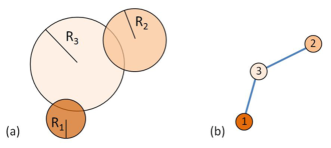
Figure 1: (Color online) Connectedness criterion for spheres with different radii. (a) The spheres of radii $R_{1}$ and $R_{2}$ overlap the sphere of radius $R_{3}$, forming links between $R_{3}$ and $R_{1}$ and between $R_{3}$ and $R_{2}$. (b) Corresponding cluster formed by nodes (sphere centers) labeled by the sphere radii and weighted links (solid lines) connecting the nodes.

III Irrelevance of closed loops for $d\rightarrow\infty$

An important aspect of the topology of random geometric graphs is represented by closed loops (or cycles) of connected nodes. The most studied loop quantity is the three-nodes cycle $c^{(3)}_{d}$, often denoted the cluster coefficient, which gives the conditional probability that two nodes are connected given that both nodes are connected to a third one. $c^{(3)}_{d}$ has been calculated for systems of spheres with identical radii and for any dimensionality Torquato2012 ; Dall2002 . The observation that $c^{(3)}_{d}$ vanishes exponentially as $d\rightarrow\infty$ indicates that random geometric graphs in large dimensions have a locally tree-like structure.

Using results from the theory of hard-sphere fluids, it is actually possible to show that, in the limit of large dimensions, closed loops are negligible also for any number of nodes and for bounded radii distributions. Random and weighted random geometric graphs have thus tree-like structures when $d\rightarrow\infty$. To see this, let us first consider the case of monodisperse spheres with radius $R_{M}$. We define an $n$-chain graph as a cluster of $n\geq 3$ nodes with $n-1$ edges such that every two consecutive edges, and only those, have a common node. We denote as end-nodes the two nodes of an $n$-chain that each have only one edge. The $n$-cycle coefficient $c^{(n)}_{d}$ is defined as the conditional probability that two nodes are connected given that they are the end-nodes of an $n$-chain. Since the spheres have identical radii, we omit the subscripts in Eq. (2), and we write the connectedness function as simply $f(r)=\theta(2R_{M}-r)$. From the definition of $c^{(n)}_{d}$, we can thus write:

$$c^{(n)}_{d}=\frac{\int dr^{(n)}f(|\mathbf{r}_{1}-\mathbf{r}_{2}|)f(|\mathbf{r}_{2}-\mathbf{r}_{3}|)\cdots f(|\mathbf{r}_{n}-\mathbf{r}_{1}|)}{\int dr^{(n)}f(|\mathbf{r}_{1}-\mathbf{r}_{2}|)f(|\mathbf{r}_{2}-\mathbf{r}_{3}|)\cdots f(|\mathbf{r}_{n-1}-\mathbf{r}_{n}|)},$$ (4)

where $dr^{(n)}=d\mathbf{r}_{1}d\mathbf{r}_{2}\cdots d\mathbf{r}_{n}$. Besides a prefactor, the above expression coincides with the cluster integral of a ring of $n$ hard-spheres of radius $R_{M}$ Loeser1991 , as the Mayer function $f_{\textrm{M}}(r)$ for a fluid of hard-spheres is just $f_{\textrm{M}}(r)=-f(r)$ TorquatoBook ; HansenMcDonald . To evaluate Eq. (4) for $d\rightarrow\infty$, we thus use known results from the theory of hard-sphere fluids in infinite dimensions. Noting that the denominator of Eq. (4) (i.e., the $n$-chain contribution) is simply $VV_{\textrm{ex}}^{n-1}$ Wyler1987 , where $V_{\textrm{ex}}=\Omega_{d}2^{d}R_{M}^{d}$ is the excluded volume for spheres of identical radius $R_{M}$, and introducing the Fourier transform $\hat{f}(\mathbf{q})$ of the connectedness function we rewrite Eq. (4) as:

$$c^{(n)}_{d}=\frac{1}{V_{\textrm{ex}}^{n-1}}\int\frac{d\mathbf{q}}{(2\pi)^{d}}\hat{f}(\mathbf{q})^{n}.$$ (5)

The integration in Eq. (5) for $d\rightarrow\infty$ has been worked out in Ref. Loeser1991 (see also Ref.Frisch1999 ), so that the $n$-cycle coefficient reduces to:

$$c^{(n)}_{d}\rightarrow\sqrt{\frac{n-2}{\pi d(n-1)}}\left(\frac{n}{n-2}\right)^{n/2}\left[\frac{n^{n-2}}{(n-1)^{n-1}}\right]^{d/2},$$ (6)

from which we see that closed loops of any number $n$ of nodes are exponentially small as $d\rightarrow\infty$, because the quantity within square brackets is less than unity for $n\geq 3$.

Let us now consider the $n$-cycle coefficient for the case of polydisperse spheres. Using Eq. (2) for the connectedness function, we generalize Eq. (4) as follows:

$$\langle c_{d}\rangle^{(n)}=\frac{\langle\mathcal{C}_{i_{1},\ldots,i_{n}}^{(n)}\rangle_{i_{1},\ldots,i_{n}}}{\langle\mathcal{V}_{i_{1},\ldots,i_{n}}^{(n)}\rangle_{i_{1},\ldots,i_{n}}},$$ (7)

where

$$\mathcal{C}_{i_{1},\ldots,i_{n}}^{(n)}=\int dr^{(n)} f_{i_{1}i_{2}}(|\mathbf{r}_{1}-\mathbf{r}_{2}|)f_{i_{2}i_{3}}(|\mathbf{r}_{2}-\mathbf{r}_{3}|)\cdots$$

$$\cdots\times f_{i_{n}i_{1}}(|\mathbf{r}_{n}-\mathbf{r}_{1}|),$$ (8)

$$\mathcal{V}^{(n)}_{i_{1},\ldots,i_{n}}=\int dr^{(n)} f_{i_{1}i_{2}}(|\mathbf{r}_{1}-\mathbf{r}_{2}|)f_{i_{2}i_{3}}(|\mathbf{r}_{2}-\mathbf{r}_{3}|)\cdots$$

$$\cdots\times f_{i_{n-1}i_{n}}(|\mathbf{r}_{n-1}-\mathbf{r}_{n}|),$$ (9)

and

$$\langle(\cdots)\rangle_{i_{1},\ldots,i_{n}}=\sum_{i_{1},\ldots,i_{n}}x_{i_{1}}x_{i_{2}}\cdots x_{i_{n}}(\cdots)$$ (10)

denotes a multiple average over the radii $R_{i_{1}},R_{i_{2}},\ldots,R_{i_{n}}$. In the appendix, we show that for bounded distributions of radii, the $n$-cycle coefficient in the limit $d\rightarrow\infty$ is such that:

$$\langle c_{d}\rangle^{(n)}\leq c^{(n)}_{d}\chi_{d}^{(n)},$$ (11)

where $c^{(n)}_{d}$ is the $n$-cycle coefficient for identical radii, Eq. (6), and $\chi_{d}^{(n)}\propto d^{a}$, where $a$ is a nonnegative constant. Since the exponential decay of $c^{(n)}$ for $d\rightarrow\infty$ is stronger than the power-law increase of $\chi_{d}^{(n)}$, we see thus that also for the case of polydisperse spheres for bounded radii distributions, the $n$-cycle coefficient vanishes for any $n\geq 3$.

IV Size of finite components

The observation made in the previous section that closed loops are irrelevant in the large dimensional limit of the Boolean model allows us to consider the components of the associated weighted random geometric graph as effectively having a tree-like structure. This leads to a considerable simplification, as we can take the formalism of the theory of random graphs (see, e.g., Refs. Newman2001 ; Albert2002 ; Boccaletti2006 ) and generalize it to the case in which nodes have weights.

IV.1 Multidegree distributions

We start by considering the multidegree distribution of a node of type $i$, defined as the probability $p_{i}(1,k_{1};2,k_{2};\dots)$ that a sphere of radius $R_{i}$ is connected to $k_{1}$ spheres of radius $R_{1}$, $k_{2}$ spheres of radius $R_{2}$, and so on. Since the radii are randomly and independently distributed among the $N$ nodes, $p_{i}(1,k_{1};2,k_{2};\dots)$ is just a product of binomial distributions $p_{ij}(k_{j})$ (with $j=1,2,\ldots$), each giving the probability that $k_{j}$ spheres of radius $R_{j}$ overlap the sphere of radius $R_{i}$:

$$p_{i}(1,k_{1};2,k_{2};\dots)=\prod_{j}p_{ij}(k_{j}),$$ (12)

with

$$p_{ij}(k_{j})=\binom{N_{j}-\delta_{i,j}}{k_{j}}(v_{\textrm{ex}}^{ij})^{k_{j}}(1-v_{\textrm{ex}}^{ij})^{N_{j}-\delta_{i,j}-k_{j}},$$ (13)

where $N_{j}$ (with $j=1,2,\ldots$) is the number of spheres of radius $R_{j}$, $v_{\textrm{ex}}^{ij}$ are the overlap probabilities given in Eq. (3), and $\delta_{i,j}$ is the Kronecker symbol.

We next consider for all $i$ the limit $N_{i}\rightarrow\infty$ such that $N_{i}/V=x_{i}\rho$ remains finite, where $\rho=N/V$ is the total number density. In this limit, Eq. (13) reduces to a Poisson distribution:

$$p_{ij}(k_{j})=\frac{z_{ij}^{k_{j}}}{k_{j}!}e^{-z_{ij}},$$ (14)

where

$$z_{ij}=\sum_{k}kp_{ij}(k)=x_{j}\rho\Omega_{d}(R_{i}+R_{j})^{d}$$ (15)

is the average number of spheres with radius $R_{j}$ that overlap a given sphere of radius $R_{i}$.

In addition to the node degree distribution $p_{i}(1,k_{1};2,k_{2};\dots)$, for the following analysis we will also need the excess node degree distribution $q_{ji}(1,k_{1};2,k_{2};\ldots)$, defined as the conditional probability that a sphere of radius $R_{j}$ is connected to $k_{l}$ spheres of radius $R_{l}$ (with $l=1,2,\ldots$), given that it is connected to a sphere of radius $R_{i}$. This task is simplified by the irrelevance of closed loops in the large dimensionality limit. In this case, indeed, if we select at random an edge connecting a node of type $j$ with a node of type $i$, the $j$ node attached to the edge is $k_{i}$ times more likely to have degree $k_{i}$ than degree $1$ with nodes of type $i$. Its degree distribution will thus be proportional to $k_{i}p_{j}(1,k_{1};2,k_{2};\dots)$. The excess degree distribution of a $j$ node that has $k_{i}$ edges with nodes of type $i$ other than the edge with the node $i$ to which is attached is thus Leicht2009 :

$$q_{ji}(1,k_{1};2,k_{2},\ldots)=\frac{(k_{i}\!+\!1)p_{j}(1,k_{1};\ldots;i,k_{i}\!+\!1;\ldots)}{\sum_{\mathbf{k}}(k_{i}\!+\!1)p_{j}(1,k_{1};\ldots;i,k_{i}\!+\!1;\ldots)},$$ (16)

where $\sum_{\mathbf{k}}=\sum_{k_{1},k_{2},\ldots}$. From Eqs. (12) and (14), $q_{ji}(1,k_{1};2,k_{2},\ldots)$ reduces simply to:

$$q_{ji}(1,k_{1};2,k_{2},\ldots) =\frac{(k_{i}+1)p_{ji}(k_{i}+1)}{z_{ji}}\prod_{l\neq i}p_{jl}(k_{l})$$

$$=\prod_{l}p_{jl}(k_{l}),$$ (17)

where we have used $(k_{i}+1)p_{ji}(k_{i}+1)=z_{ji}p_{ji}(k_{i})$. Equation (IV.1) states thus the well-known property that the excess degree distribution coincides with the node degree distribution when this is Poissonian Newman2001 .

IV.2 Mean cluster size in the subcritical regime

We exploit now the statistical irrelevance of closed loops discussed in Sec. III to find the mean size $S$ of finite clusters of connected spheres as $d\rightarrow\infty$. In doing so, we shall first keep the form of the degree distributions unspecified, and apply Eqs. (14) and (IV.1) only at the end of the calculation.

Let us start by considering a randomly selected node that has probability $x_{i}$ of being occupied by a sphere of radius $R_{i}$. Due to the general tree-like structure of the graph, the cluster to which the selected node belongs is formed by branches attached to the node according to the degree distribution $p_{i}(1,k_{1};2,k_{2};\ldots)$, as schematically shown in Fig. 2. The mean size $S_{i}$ of the cluster to which the selected node belongs is thus:

$$S_{i}=x_{i}+x_{i}\sum_{\mathbf{k}}p_{i}(1,k_{1};2,k_{2};\ldots)\sum_{j}k_{j}T_{ij},$$ (18)

where $T_{ij}$ is the mean cluster size of one of the $k_{j}$ branches attached to the selected node. Since the clusters have a tree-like structure, $T_{ij}$ is given by the mass (unity) of one neighbor of the selected node, plus the mean cluster size of each of the remaining subbranches attached to the neighbor. To find $T_{ij}$, we thus need the excess degree distribution $q_{ji}(1,k_{1};2,k_{2};\ldots)$ of a sphere of radius $R_{j}$ connected to the selected node of type $i$:

$$T_{ij}=1+\sum_{\mathbf{k}}q_{ji}(1,k_{1};2,k_{2};\ldots)\sum_{l}k_{l}T_{jl}.$$ (19)

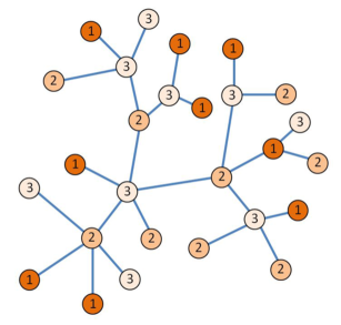
Figure 2: (Color online) Schematic representation of a finite tree-like cluster formed by connected spheres of radii $R_{1}$, $R_{2}$, and $R_{3}$. Each node label corresponds to the value of the radius of the sphere attached to the node.

Equations (18) and (19) are quite general, as they apply also to tree-like graphs with degree distributions that are not reducible to a multiplication of Poissonian probabilitites. Interestingly, similar equations are found in the calculation of finite size components of multigraphs (also denoted multiplex networks), formed by different networks, each having particular node properties, coupled together Leicht2009 ; Allard2009 . The Boolean-Poisson model with random radii can thus be viewed also as a particular type of multigraph, in which each individual network is constituted by nodes occupied by spheres of a given radius.

Let us now use the results of Sec. IV.1 and rewrite Eqs. (18) and (19) by substituting $p_{i}(1,k_{1};2,k_{2};\ldots)$ and $q_{ji}(1,k_{1};2,k_{2};\ldots)$ with, respectively, Eqs. (12) and (IV.1):

$$S_{i} =x_{i}+x_{i}\sum_{j}\sum_{k}kp_{ij}(k)T_{j}=x_{i}+x_{i}\sum_{j}z_{ij}T_{j},$$ (20)

$$T_{j} =1+\sum_{l}\sum_{k}kp_{jl}(k)T_{l}=1+\sum_{l}z_{jl}T_{l},$$ (21)

where we have used Eq. (15) and the fact that $T_{ij}$ depends only on the neighbor ($j$) of the selected node, i.e., $T_{ij}=T_{j}$.

The mean cluster size is given by $S=\sum_{i}S_{i}$, which from Eq. (20) reduces to: $S=1+\sum_{ij}x_{i}z_{ij}T_{j}$. This relation is obtained also if we multiply both sides of Eq. (21) by $x_{j}$ and sum over $j$. We can thus write:

$$S=\sum_{j}x_{j}T_{j},$$ (22)

which states that $S$ is just the average over the sphere radii of the mean cluster size of the branches.

IV.3 Equivalence with the Ornstein-Zernike equation for the pair-connectedness

In continuum percolation theory, cluster statistics are often studied using the formalism of pair-connectedness correlation functions TorquatoBook ; Coniglio1977 ; Stell1996 , which exploits well developed techniques of liquid state theory. This method has been recently used to studying percolation of monodisperse spheres in large dimensions Torquato2012 .

As long as closed loops can be neglected, the network formalism discussed above and the pair-connectedness functions method give identical results, provided that the second-virial approximation is taken. To see how this equivalence holds true for the Boolean model in large dimensions, let us first consider the pair-connectedness function $P_{ij}(\mathbf{r}-\mathbf{r}^{\prime})$, defined such that $x_{i}x_{j}\rho^{2}P_{ij}(\mathbf{r}-\mathbf{r}^{\prime})d\mathbf{r}d\mathbf{r}^{\prime}$ is the probability of finding two spheres of radii $R_{i}$ and $R_{j}$ within the volume elements $d\mathbf{r}$ and $d\mathbf{r}^{\prime}$ centered respectively in $\mathbf{r}$ and $\mathbf{r}^{\prime}$, given that they belong to the same cluster. The mean cluster size $S$ is given in terms of $P_{ij}(\mathbf{r}-\mathbf{r}^{\prime})$ by the following relationOtten2011 :

$$S=1+\rho\sum_{i,j}x_{i}x_{j}P_{ij},$$ (23)

where $P_{ij}=\int d\mathbf{r}P_{ij}(\mathbf{r})$. $P_{ij}$ is the solution of the pair connectedness analog of the Ornstein-Zernike equation of the liquid state theory of fluids:

$$P_{ij}=C_{ij}+\rho\sum_{l}x_{l}C_{il}P_{lj},$$ (24)

where $C_{ij}=\int d\mathbf{r}C_{ij}(\mathbf{r})$ is the volume integral of the direct pair connectedness function $C_{ij}(\mathbf{r})$, which describes short-range connectivity correlations. Let us introduce the quantity $\widetilde{T}_{i}$ defined as:

$$\widetilde{T}_{i}=1+\rho\sum_{j}x_{j}P_{ij}.$$ (25)

The use of the above expression reduces Eq. (23) to:

$$S =\sum_{i}x_{i}+\rho\sum_{i,j}x_{i}x_{j}P_{ij}=\sum_{i}x_{i}\left(1+\rho\sum_{j}x_{j}P_{ij}\right)$$

$$=\sum_{i}x_{i}\widetilde{T}_{i},$$ (26)

while inserting Eq.(24) into Eq. (25) leads to:

$$\widetilde{T}_{i} =1+\rho\sum_{j}x_{j}\left(C_{ij}+\rho\sum_{l}x_{l}C_{il}P_{lj}\right)$$

$$=1+\rho\sum_{j}x_{j}C_{ij}+\rho\sum_{j}x_{j}C_{ij}(\widetilde{T}_{j}-1)$$

$$=1+\rho\sum_{j}x_{j}C_{ij}\widetilde{T}_{j}.$$ (27)

We see that Eqs. (IV.3) and (IV.3) are identical to respectively Eqs. (22) and (21) if we identify $\rho x_{j}C_{ij}$ with $z_{ij}$. From Eq. (15), we obtain thus:

$$C_{ij}=\frac{z_{ij}}{\rho x_{j}}=\Omega_{d}(R_{i}+R_{j})^{d},$$ (28)

which corresponds to take the volume integral of the second-virial approximation $C_{ij}(\mathbf{r})=C_{ij}^{(2)}(\mathbf{r})=f_{ij}(r)$ for the direct pair-connectedness function. This is not surprising, because in the density expansion of the direct pair-connectedness function, $C_{ij}(\mathbf{r})=\sum_{n\geq 2}\rho^{n-2}C_{ij}^{(n)}(\mathbf{r})$, the terms with $n\geq 3$ contain at least one closed loop.

V Universality of the percolation threshold

We proceed to find the percolation threshold for the Boolean-Poisson model of polydisperse spheres in the large dimensionality limit. We shall consider the case of bounded distributions of the radii, for which we have shown in Sec. III that closed loops of connected particles can be neglected for $d\rightarrow\infty$, and Eqs. (21) and (22) are valid. To measure the sphere concentration we introduce the dimensionless density

$$\eta=\rho\Omega_{d}\langle R^{d}\rangle_{R}=\rho\Omega_{d}\sum_{i}x_{i}R_{i}^{d}.$$ (29)

The percolation threshold $\eta_{c}$ is defined as the smallest value of $\eta$ such that $S$ diverges. This definition is equivalent to finding the smallest pole of Eq. (21), if it exists.

V.1 Discrete radii distributions

We first consider the case in which the spheres have a finite number $M$ of radii:

$$\rho(R)=\sum_{i=1}^{M}x_{i}\delta(R-R_{i}),$$ (30)

so that using Eqs. (15), (21) and (22) we rewrite the equations for the mean cluster size as:

$$S =\sum_{i=1}^{M}x_{i}T_{i},$$ (31)

$$T_{i} =1+\rho\Omega_{d}\sum_{j=1}^{M}x_{j}(R_{i}+R_{j})^{d}T_{j}.$$ (32)

Without loss of generality, we assume that $R_{M}$ is strictly the largest radius out of the $M$ possible values of the radii, and we introduce $q_{i}=R_{i}/R_{M}$, which takes values smaller than the unity for all $i\neq M$. For large $d$, the dimensionless density $\eta$ reduces to:

$$\eta =\rho\Omega_{d}\sum_{i=1}^{M}x_{i}R_{i}^{d}=\rho\Omega_{d}R_{M}^{d}\left[x_{M}+\sum_{i=1}^{M-1}x_{i}q_{i}^{d}\right]$$

$$\rightarrow\rho\Omega_{d}R_{M}^{d}x_{M},$$ (33)

because $q_{i}^{d}$ goes exponentially to zero as $d\rightarrow\infty$ when $i\neq M$, and Eq. (32) becomes:

$$T_{i}=1+2^{d}\eta\frac{1}{x_{M}}\sum_{j}x_{j}\left(\frac{q_{i}+q_{j}}{2}\right)^{d}T_{j}.$$ (34)

We note that $\left(\frac{q_{i}+q_{j}}{2}\right)^{d}$ is vanishingly small as $d\rightarrow\infty$ unless $i=j=M$, for which it takes the value $1$. The smallest pole of Eq. (34) for large $d$ is thus the solution of:

$$T_{i}=1+2^{d}\eta T_{M}\delta_{i,M},$$ (35)

where $\delta_{i,j}$ is the Kronecker delta. Equation (35) is solved by $T_{M}=1/(1-2^{d}\eta)$ and $T_{i}=1$ for $i\neq M$, so that the mean cluster size (31) becomes:

$$S=\sum_{i=1}^{M-1}x_{i}+x_{M}T_{M}=\frac{x_{M}}{1-2^{d}\eta},$$ (36)

which diverges when

$$\eta\rightarrow\eta_{c}=\frac{1}{2^{d}}.$$ (37)

The above expression for $\eta_{c}$ holds true for any sequence of occupation fractions $x_{i}$, independent of dimensionality, provided that $x_{M}\neq 0$. In particular, Eq. (37) confirms and extends to $M>2$ the finding of a previous report that spheres with two different radii have a universal critical threshold in infinite dimensions Gouere2014 . Note that $\eta_{c}=1/2^{d}$ is also the limit for infinite dimensions of the percolation threshold of monodisperse spheres with radius $R_{M}$, whose mean cluster size is given by Eq. (36) with $x_{M}=1$.

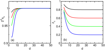
Figure 3: (Color online) (a) Percolation threshold $\eta_{c}$ in units of the asymptotic value $2^{-d}$ as a function of dimensionality for a discrete distribution of radii with $M=2$ and $R_{1}/R_{2}=1/2$. In this case Eq. (32) is a system of two linear equations so that $\eta_{c}$ can be calculated exactly for any $d$. $x_{2}=0.8$, 0.6$,0.4$, and $0.2$ from the uppermost to the lowermost curves. (b) Corresponding values of the critical coordination number $z_{c}$. As $d\rightarrow\infty$, $z_{c}$ tends asymptotically to $x_{2}$.

The origin of the universality of $\eta_{c}$ can be traced back to the divergence of $T_{M}$, which indicates that the onset of a giant component of connected polydisperse spheres is established only by the subset of spheres with the maximum radius when $d\rightarrow\infty$. In other words, at $d\rightarrow\infty$ the contribution to percolation of the smaller spheres vanishes, and the resulting $\eta_{c}$ is the critical threshold for a system of monodisperse spheres of radius $R_{M}$. Following the observation that systems of polydisperse spheres with $M$ different radii can be interpreted as a multinetwork of coupled $M$ subnetworks (see Sec. IV.2), we see that Eq. (35) is equivalent to decoupling the subnetworks associated with each radius, and that long-range connectivity arises only from the network formed by spheres with radius $R_{M}$.

One interesting consequence of the irrelevance of smaller radii at percolation is that the critical average connectivity per particle,

$$z_{c}=\sum_{i,j}x_{i}x_{j}\rho_{c}\Omega_{d}(R_{i}+R_{j})^{d},$$ (38)

reduces for $d\rightarrow\infty$ to:

$$z_{c}=2^{d}\rho_{c}\Omega_{d}R_{M}^{d}\sum_{i,j}x_{i}x_{j}\left(\frac{q_{i}+g_{j}}{2}\right)^{d}\rightarrow 2^{d}\eta_{c}x_{M}=x_{M},$$ (39)

where $\rho_{c}$ is the critical number density. For $x_{M}<1$, the critical average connectivity is thus less than the unity for $d\rightarrow\infty$, which must be contrasted to $z_{c}\geq 1$ for systems constituting only of monodisperse spheres in any dimension Torquato2012 .

For the binary case ($M=2$), Eq. (32) reduces to a system of two linear equations that can be solved exactly for any $d$. The resulting $\eta_{c}$ and $z_{c}$ are shown in Figs. 3(a) and 3(b), respectively, for $R_{2}=2R_{1}$ and different values of the fraction $x_{2}$ of spheres of radius $R_{2}$. The asymptotic limits $\eta_{c}=2^{-d}$ and $z_{c}=x_{2}$ are recovered for sufficiently large values of $d$.

V.2 Continuous radii distributions

Let us now consider the case in which the radii distribution $\rho(R)$ is a continuous bounded function independent of $d$. We again denote by $R_{M}<\infty$ the maximum allowed radius, so that $\rho(R)=0$ for $R>R_{M}$, and we rewrite the equations for the mean cluster size in terms of continuous variables of the radii:

$$S =\langle T(R)\rangle_{R},$$ (40)

$$T(R) =1+\rho\Omega_{d}\langle(R+R^{\prime})^{d}T(R^{\prime})\rangle_{R^{\prime}},$$ (41)

where $\langle(\cdots)\rangle_{R}=\int_{0}^{R_{M}}dR\rho(R)(\cdots)$. We expand the binomial power $(R+R^{\prime})^{d}$ and use $\eta=\rho\Omega_{d}\langle R^{d}\rangle_{R}$ to write:

$$T(R)=1+\eta\sum_{k=0}^{d}\binom{d}{k}\frac{R^{d-k}}{\langle R^{d}\rangle_{R}}\langle R^{k}T(R)\rangle_{R}.$$ (42)

If we multiply both sides of Eq. (42) by $R^{n}/\langle R^{n}\rangle_{R}$, with $n=1$, $2$, $\ldots$, $d$, and average over $R$ we arrive at:

$$t(n)=1+\eta\sum_{k=0}^{d}\binom{d}{k}\frac{\langle R^{n+d-k}\rangle_{R}\langle R^{k}\rangle_{R}}{\langle R^{d}\rangle_{R}\langle R^{n}\rangle_{R}}t(k),$$ (43)

where

$$t(n)=\frac{\langle R^{n}T(R)\rangle_{R}}{\langle R^{n}\rangle_{R}}.$$ (44)

From Eqs. (40) and (44) we see that the mean cluster size can be obtained from $S=t(0)$.

To solve Eq. (43), we note that for large $d$ the binomial coefficient is strongly peaked at $k=d/2$ and takes the asymptotic form

$$\binom{d}{k}\simeq 2^{d}\sqrt{\frac{2}{\pi d}}e^{-\frac{2}{d}(k-d/2)^{2}}=\frac{2^{d+1}}{d}g\!\left(\frac{2k}{d}-1,\frac{1}{\sqrt{d}}\right),$$ (45)

where $g(x,\sigma)=\exp(-x^{2}/2\sigma^{2})/\sqrt{2\pi\sigma^{2}}$ is the Gaussian function. Provided that the radii distribution is bounded, the binomial coefficent dominates the $k$-dependence of the kernel. To see this, let us consider the $m$-th moment $\langle R^{m}\rangle_{R}=R_{M}^{m}\int_{0}^{1}dy\rho(y)y^{m}$, where $y=R/R_{M}$. For large $m$ the main contribution to the integral comes from $y$ close to $1$. Thus we make the quite general assumption that for $y\rightarrow 1$, the radii distribution behaves as $\rho(y)\propto(1-y)^{\alpha-1}$, with $\alpha>0$. Setting $t=m(1-y)$ for large $m$, we find

$$\langle R^{m}\rangle_{R} \propto\frac{R_{M}^{m}}{m^{\alpha}}\int_{0}^{m}\!dt\,t^{\alpha-1}(1-t/m)^{m}$$

$$\simeq\frac{R_{M}^{m}}{m^{\alpha}}\int_{0}^{\infty}\!dt\,t^{\alpha-1}e^{-t}=\frac{R_{M}^{m}}{m^{\alpha}}\Gamma(\alpha),$$ (46)

so that for large $k$ the term $\langle R^{n+d-k}\rangle_{R}\langle R^{k}\rangle_{R}$ in Eq. (43) is proportional to $R_{M}^{n+d}/[(n+d-k)k]^{\alpha}$, which has a much weaker $k$-dependence than Eq. (45). Next, we introduce $s=2n/d$ and $s^{\prime}=2k/d$, which we treat as continuous variables for $d\rightarrow\infty$, and we replace the sum over $k$ by an integral over $s^{\prime}$: $\sum_{k=0}^{d}\rightarrow\frac{d}{2}\int_{0}^{2}ds^{\prime}$. If we denote $\tilde{t}(s)=t(ds/2)$ and $\tilde{t}(s^{\prime})=t(ds^{\prime}/2)$, Eq. (43) becomes:

$$\tilde{t}(s)=1+2^{d}\eta\int_{0}^{2}ds^{\prime} \left[g\!\left(s^{\prime}-1,\frac{1}{\sqrt{d}}\right)\right.$$

$$\left.\times\frac{\langle R^{d[1+(s-s^{\prime})/2]}\rangle_{R}\langle R^{ds^{\prime}/2}\rangle_{R}}{\langle R^{d}\rangle_{R}\langle R^{ds/2}\rangle_{R}}\tilde{t}(s^{\prime})\right].$$ (47)

Since $g(s^{\prime}-1,1/\sqrt{d})\rightarrow\delta(s^{\prime}-1)$ for $d\rightarrow\infty$, the above expression reduces to:

$$\tilde{t}(s)=1+\eta 2^{d}\frac{\langle R^{d(1+s)/2}\rangle_{R}\langle R^{d/2}\rangle_{R}}{\langle R^{d}\rangle_{R}\langle R^{ds/2}\rangle_{R}}\tilde{t}(1),$$ (48)

from which we obtain the mean cluster size:

$$S=\tilde{t}(0)=1+\eta 2^{d}\frac{\langle R^{d/2}\rangle_{R}^{2}}{\langle R^{d}\rangle_{R}}\tilde{t}(1).$$ (49)

Setting $s=1$ in Eq. (48), we find $\tilde{t}(1)=(1-2^{d}\eta)^{-1}$, so that we arrive finally at:

$$S=\frac{1}{1-2^{d}\eta}\frac{\langle R^{d/2}\rangle_{R}^{2}}{\langle R^{d}\rangle_{R}},$$ (50)

which, as found for the case of discrete distributions, diverges at

$$\eta\rightarrow\eta_{c}=\frac{1}{2^{d}},$$ (51)

independently of the particular form of the bounded distribution $\rho(R)$.

Using Eq. (45) and considering the weak dependence of the moments of $R$, we readily obtain the large dimensional limit of the critical average connectivity per particle:

$$z_{c} =\rho_{c}\Omega_{d}\langle(R+R^{\prime})^{d}\rangle_{R,R^{\prime}}=\eta_{c}\sum_{k=0}^{d}\binom{d}{k}\frac{\langle R^{k}\rangle_{R}\langle R^{d-k}\rangle_{R}}{\langle R^{d}\rangle_{R}}$$

$$\rightarrow\frac{\langle R^{d/2}\rangle_{R}^{2}}{\langle R^{d}\rangle_{R}},$$ (52)

from which we see that $z_{c}\leq 1$ for any bounded distribution of the radii. Note that from Eq. (V.2) we recover $z_{c}=x_{M}$ when $\rho(R)$ is given by Eq. (30).

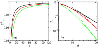
Figure 4: (Color online) (a) Dimensional dependence of the percolation threshold $\eta_{c}$ in units of the asymptotic value $2^{-d}$ obtained from a numerical solution of Eq. (43) for rectangular (upper curve), semicircular (middle curve), and triangular (lower curve) distributions of the sphere radii. (b) Corresponding critical average connectivity per particle $z_{c}$ (solid curves). Dashed lines are the asymptotic results for $d\gg 1$: $z_{c}=4/d$ (rectangular distribution), $z_{c}=32/(\sqrt{\pi}d^{3/2})$ (semicircular distribution), and $z_{c}=32/d^{2}$ (triangular distribution).

We complete this section by showing how the percolation threshold obtained from Eqs. (40) and (41) evolves towards the asymptotic value $\eta_{c}=2^{-d}$ as $d$ increases. Toward that end, we consider radii distributions of rectangular, semicircular, and triangular shapes, given respectively by $\rho(R)=1/R_{M}$, $\rho(R)=4\sqrt{(R_{M}/2)^{2}+(R-R_{M}/2)^{2}}/\pi$, and $\rho(R)=2(R_{M}-R)/R_{M}^{2}$, for $R\leq R_{M}$ and zero otherwise. We calculate $\eta_{c}$ from the smallest pole of $S=t(0)$ obtained from a numerical solution of Eq. (43). The resulting thresholds are very close to $2^{-d}$ for all $d$ considered, and they approach the asymptotic limit from below, as shown in Fig. 4(a). For the same cases of Fig. 4(a), we have calculated also the $d$-dependence of $z_{c}$, shown in Fig. 4(b) by solid lines, which we compare with the asymptotic limits (dashed lines) $z_{c}=4/d$, $z_{c}=32/(\sqrt{\pi}d^{3/2})$, and $z_{c}=32/d^{2}$ obtained from Eq. (V.2) for rectangular, semicircular, and triangular distributions of the radii, respectively.

VI The case of unbounded distribution of the radii

Having established that $\eta_{c}$ is universal as $d\rightarrow\infty$ for bounded (and independent of $d$) distributions of the radii, it is natural to ask if universality holds true also when $\rho(R)$ is unbounded. Although we have shown the irrelevance of closed loops limited to the case of bonded distributions, we shall nevertheless assume that $n$-cycle coefficients are negligible also for unbounded $\rho(R)$, and that graph components have a tree-like structure. Let us consider the specific case of a lognormal distribution function:

$$\rho(R)=\frac{1}{\sqrt{2\pi}\sigma R}\exp\!\left[-\frac{\ln^{2}(R/R_{0})}{2\sigma^{2}}\right],$$ (53)

where $R\in[0,\infty)$, $R_{0}$ is the median radius, and $\sigma$ is the standard deviation of $\ln(R)$. Equation (53) is an interesting case-study, as the resulting $\eta_{c}$ and $z_{c}$ for asymptotically large $d$ can be found analytically. Using the $k$-th moment $\langle R^{k}\rangle_{R}=R_{0}^{k}\exp(\sigma^{2}k^{2}/2)$, Eq. (43) becomes:

$$t(n)=1+\eta\sum_{k=0}^{d}\binom{d}{k}e^{\frac{1}{2}\sigma^{2}[(n+d-k)^{2}+k^{2}-n^{2}-d^{2}]}t(k),$$ (54)

from which we express the mean cluster size as:

$$S=t(0)=1+\eta\sum_{k=0}^{d}\binom{d}{k}e^{\sigma^{2}k(k-d)}t(k).$$ (55)

For sufficiently large $d$, the only nonvanishing terms of the summation are those with $k=0$ and $k=d$, so that:

$$S=1+\eta[S+t(d)],$$ (56)

where from Eq. (54) $t(d)$ is given by:

$$t(d)=1+\eta\sum_{k=0}^{d}\binom{d}{k}e^{\sigma^{2}(d-k)^{2}}t(k).$$ (57)

For $d\rightarrow\infty$, $t(d)$ tends asymptotically to $t(d)=1+\eta e^{\sigma^{2}d^{2}}t(0)$, as the term with $k=0$ dominates the sum over $k$ in Eq. (57). We thus find that the mean cluster size, Eq. (56), reduces to:

$$S=\frac{1+\eta}{1-\eta-\eta^{2}e^{\sigma^{2}d^{2}}},$$ (58)

which diverges at the asymptotical critical value,

$$\eta\rightarrow\eta_{c}=e^{-\frac{1}{2}\sigma^{2}d^{2}}.$$ (59)

The corresponding critical coordination number is

$$z_{c} =\eta_{c}\sum_{k=0}^{d}\binom{d}{k}\frac{\langle R^{k}\rangle_{R}\langle R^{d-k}\rangle_{R}}{\langle R^{d}\rangle_{R}}=\eta_{c}\sum_{k=0}^{d}\binom{d}{k}e^{\sigma^{2}k(k-d)}$$

$$\rightarrow 2\eta_{c},$$ (60)

where we have again used the fact that for large $d$ only the terms $k=0$ and $k=d$ contribute to the summation.

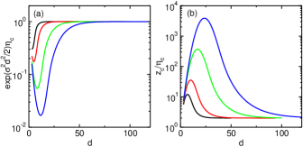
Figure 5: (Color online) (a) Dimensional dependence of the percolation threshold $\eta_{c}$ in units of the asymptotic value $\exp(-\sigma^{2}d^{2}/2)$ for a lognormal distribution of the radii obtained from a numerical solution of Eq. (54); $\sigma=0.25$, $0.3$, $0.4$, and $0.5$ from the lowermost to the uppermost curves. (b) Critical average connectivity per particle $z_{c}$ for $\sigma=0.25$, $0.3$, $0.4$, and $0.5$ from the uppermost to the lowermost curves. All curves tend to $z_{c}/\eta_{c}\rightarrow 2$ as $d\rightarrow\infty$.

As evidenced in Eq. (59), the percolation threshold for infinite dimensions is no longer universal, as it depends on the parameter $\sigma$ of the log-normal distribution. Interestingly, from Eq. (59) we also see that $\eta_{c}$ can be smaller than the critical threshold of monodisperse spheres ($\eta_{c}=2^{-d}$), contrary to what is expected in finite dimensions Meester1994 . We note that a critical threshold smaller than the monodisperse sphere limit in large dimensions has been found also for the case of radii distributions with $d$-dependent weights Gouere2013 ; Gouere2014 .

To verify the accuracy of Eq. (59), we compare it with the threshold obtained by solving numerically Eq. (54). As $d$ increases, the asymptotic limit $\eta_{c}=e^{-\frac{1}{2}\sigma^{2}d^{2}}$ is reached more rapidly when $\sigma$ is larger, as shown in Fig. 4(a). From inspection of Eq. (55) we see that this behavior is due to the competition between $e^{\sigma^{2}k(k-d)}$ and the maximum value $\sim 2^{d}$ of the binomial coefficient at $k=d/2$: the latter is suppressed by the exponential function when $d>4\ln(2)/\sigma^{2}$. From numerical calculation of $z_{c}$, shown in Fig. 5(b) for the same $\sigma$ values of Fig. 5(a), we see that also the asymptotic formula for $z_{c}$, Eq. (VI), is verified.

VII Lower bound on the percolation threshold

Having established that Eqs. (21) and (22) give asymptotic limits of the critical threshold $\eta_{c}$ as $d\rightarrow\infty$, we show now that the same equations provide also a lower bound on $\eta_{c}$ for any dimensionality. Toward that end, we take the pair-connectedness function $P_{ij}(\mathbf{r})$ considered in Sec. IV.3, and we extend to the polydisperse sphere case the inequality formulated in Ref. Given1990 :

$$P_{ij}(\mathbf{r})\leq f_{ij}(r)+\rho\sum_{l}x_{l}\int d\mathbf{r}^{\prime}f_{il}(|\mathbf{r}-\mathbf{r}^{\prime}|)P_{lj}(\mathbf{r}^{\prime}),$$ (61)

where $f_{ij}(r)$ is the connectedness function given in Eq. (2). The above expression applies to any dimensionality, and following Ref. Torquato2012 , where Eq. (61) has been used for the monodisperse sphere case, it enable us to find a lower bound on the percolation threshold. To see this, we take the volume integral of Eq. (61),

$$P_{ij}\leq V_{\textrm{ex}}^{ij}+\rho\sum_{l}x_{l}V_{\textrm{ex}}^{il}P_{lj},$$ (62)

where $V_{\textrm{ex}}^{ij}=\int d\mathbf{r}f_{ij}(r)=\Omega_{d}(R_{i}+R_{j})^{d}$, and we use Eqs. (25) to find:

$$\widetilde{T}_{i}\leq 1+\rho\sum_{j}x_{j}V_{\textrm{ex}}^{ij}\widetilde{T}_{j}=1+\sum_{j}z_{ij}\widetilde{T}_{j},$$ (63)

which together with Eq. (IV.3) gives an upper bound for the mean cluster size:

$$S=\sum_{i}x_{i}\widetilde{T}_{i}\leq\sum_{i}x_{i}T_{i},$$ (64)

where $T_{i}$ is the solution of Eq. (21). From the inequality of Eq. (64), we see that the value of $\eta$ such that $\sum_{i}x_{i}T_{i}$ diverges identifies a lower bound on the percolation threshold for any $d$. The solid lines plotted in Figs. 3(a)-5(a) represent thus lower bounds on $\eta_{c}$ for the different radii distribution functions considered in this work. As $d$ increases, these lower bounds tend asymptotically to the infinite dimensional limit $2^{-d}$ for bounded radii distributions and to $\exp(-\sigma^{2}d^{2}/2)$ for lognormal radii distributions. Finally, we note that Eq. (64) implies also that the values of $z_{c}$ shown in Figs.  3(b)-5(b) are lower bounds on the critical connectivity for any dimensionality.

VIII Summary and discussion

We have considered random dispersions of penetrable $d$-dimensional spheres with distributed radii in terms of weighted random geometric graphs, where nodes represent sphere centers and edges connect nodes of overlapping spheres with probability weighted by the sphere radii. For bounded distribution of the radii, we have shown that closed loops of connected spheres can be neglected in the limit $d\rightarrow\infty$ and that graph components have thus tree-like structure. Analysis of the mean cluster size reveals that the asymptotic percolation threshold is universal and coincides with the threshold $\eta_{c}=2^{-d}$ found for the case of monodisperse spheres in high dimensions. This result confirms and extends a previous finding on the percolation of $d\rightarrow\infty$ spheres with two different radii Gouere2013 ; Gouere2014 . Furthermore, we show that the asymptotic critical connectivity per particle $z_{c}$, though dependent on the shape of the radii distribution function, is less than unity and approaches $z_{c}\rightarrow 1$ for spheres of identical radii.

We have also studied critical connectivity for spheres with radii distributed according to a $d$-independent lognormal function, which is a treatable example of unbounded distribution. Assuming that clusters have a tree-like structure, we find that the percolation threshold $\eta_{c}$ depends on the shape of the log-normal distribution and, interestingly, that $\eta_{c}$ for $d\rightarrow\infty$ can be smaller that the threshold for monodisperse spheres, in contrast to what is expected at finite dimensions Meester1994 .

Before concluding, let us speculate on the percolation threshold in homogeneous fluids of polydisperse spheres with impenetrable cores (cherry-pit model TorquatoBook ). In finite dimensions, correlations between the cores preclude writing the multi-degree distribution as a product of Poisson distributions, as done in Sec. IV.1, because the $N$-particle distribution function $g_{N}(\mathbf{r}_{1},\mathbf{r}_{2},\ldots,\mathbf{r}_{N})$ depends on the relative positions of the core centers HansenMcDonald . However, in the limit of infinite dimensions and for small densities, $g_{N}(\mathbf{r}_{1},\mathbf{r}_{2},\ldots,\mathbf{r}_{N})$ asymptotically factorizes into a product of $\theta$-functions that are unity for pair distances beyond the hard-core diameter Torquato2006 . The multi-degree distribution for $d\rightarrow\infty$ can thus still be written as a product of Poisson distributions, with the average number of contacts unaltered by the presence of the hard-cores if the penetrable shells are non-vanishing. With the same reasoning, closed loops are expected to be negligible and graphs are still dominated by tree-like components. For non-zero penetrable shells, therefore we expect the same asymptotic results for $\eta_{c}$ as those obtained for the case of penetrable hyperspheres.

Appendix A Irrelevance of $\langle c_{d}\rangle^{(n)}$ for $d\rightarrow\infty$

In this appendix, we show that when the radii distribution is independent of $d$ and bounded [that is, when $\rho(R)=0$ for any $R>R_{M}$, with $R_{M}<\infty$], the $n$-cycle coefficient for polydisperse spheres, defined in Eqs. (7)-(III), vanishes for $d\rightarrow\infty$.

Since $R_{M}$ is the maximum radius of the distribution, the connectedness functions in the integrand of Eq. (III) are such that $f_{ij}(r)\leq f(r)=\theta(2R_{M}-r)$ for any $i$ and $j$. We can thus write:

$$\mathcal{C}_{i_{1},\ldots,i_{n}}^{(n)}\leq\int dr^{(n)}f(|\mathbf{r}_{1}-\mathbf{r}_{2}|)f(|\mathbf{r}_{2}-\mathbf{r}_{3}|)\cdots f(|\mathbf{r}_{n}-\mathbf{r}_{1}|),$$ (65)

which, when substituted in Eq. (7), gives:

$$\langle c_{d}\rangle^{(n)}\leq c^{(n)}_{d}\frac{VV_{\textrm{ex}}^{n-1}}{\langle\mathcal{V}_{i_{1},\ldots,i_{n}}^{(n)}\rangle_{i_{1},\ldots,i_{n}}},$$ (66)

where $V_{\textrm{ex}}=2^{d}\Omega_{d}R_{M}^{d}$, and $c^{(n)}_{d}$ is the $n$-cycle coefficient for identical radii given in Eq. (6). Next, we perform the integrations over $\mathbf{r}_{1},\ldots,\mathbf{r}_{n}$ in Eq. (III) to find:

$$\mathcal{V}_{i_{1},\ldots,i_{n}}^{(n)} =V\prod_{j=1}^{n-1}V_{\textrm{ex}}^{i_{j},i_{j+1}}=V\Omega_{d}^{n-1}\prod_{j=1}^{n-1}(R_{i_{j}}+R_{i_{j+1}})^{d}$$

$$=V\Omega_{d}^{n-1}\prod_{j=1}^{n-1}\left[\sum_{k_{j}=0}^{d}\binom{d}{k_{j}}R_{i_{j}}^{k_{j}}R_{i_{j+1}}^{d-k_{j}}\right],$$ (67)

where in the last equality we have expanded the binomial powers. In performing the average over $R_{i_{1}},\ldots,R_{i_{n}}$, we must group the contributions with equal radius variables and average them independently of the other radii. Denoting a general $m$-th moment as $\langle R^{m}\rangle_{R}$, we obtain:

$$\langle\mathcal{V}_{i_{1},\ldots,i_{n}}^{(n)}\rangle_{i_{1},\ldots,i_{n}} =V\Omega_{d}^{n-1}\sum_{k_{1}=0}^{d}\binom{d}{k_{1}}\cdots\sum_{k_{n-1}=0}^{d}\binom{d}{k_{n-1}}$$

$$\times\langle R^{k_{1}}\rangle_{R}\langle R^{d-k_{1}+k_{2}}\rangle_{R}\langle R^{d-k_{2}+k_{3}}\rangle_{R}\cdots$$

$$\cdots\langle R^{d-k_{n-2}+k_{n-1}}\rangle_{R}\langle R^{d-k_{n-1}}\rangle_{R}.$$ (68)

Following Sec. V.2, we approximate for large $d$ the binomial coefficients by Gaussian functions centered at $d/2$, and we replace the sums by integrals, so that for $d\rightarrow\infty$, $\sum_{k_{j}=0}^{d}\binom{d}{k_{j}}\rightarrow 2^{d}\int_{0}^{2}ds_{j}\delta(s_{j}-1)$, where $s_{j}=2k_{j}/d$ and $j=1,\ldots,n-1$. Equation (A) reduces in this way to:

$$\langle\mathcal{V}_{i_{1},\ldots,i_{n}}^{(n)}\rangle_{i_{1},\ldots,i_{n}}\rightarrow V\Omega_{d}^{n-1}2^{(n-1)d}\langle R^{d/2}\rangle_{R}^{2}\langle R^{d}\rangle_{R}^{n-2},$$ (69)

so that Eq. (66) becomes:

$$\langle c_{d}\rangle^{(n)}\leq c^{(n)}_{d}\chi_{d}^{(n)},$$ (70)

where

$$\chi_{d}^{(n)}=\frac{R_{M}^{(n-1)d}}{\langle R^{d/2}\rangle_{R}^{2}\langle R^{d}\rangle_{R}^{n-2}}.$$ (71)

For continuous radii distributions, we assume that $\rho(R)\propto(R_{M}-R)^{\alpha-1}$ with $\alpha>0$ for $R\rightarrow R_{M}$, as done in Sec. V.2. Using Eq. (V.2) we thus find $\chi_{d}^{(n)}\propto d^{n\alpha}$. For discrete distributions as in Eq. (30), it is straightforward to show from Eq. (71) that $\chi_{d}^{(n)}\rightarrow 1/(x_{M})^{n}$ for large $d$. We have thus arrived at the result that $\chi_{d}^{(n)}$ increases with $d$ at most as a power-law, leading to $\langle c_{d}\rangle^{(n)}\rightarrow 0$ as $d\rightarrow\infty$, due to the exponential vanishing of $c^{(n)}_{d}$.

References

- (1) D. Stauffer and A. Aharony, Introduction to Percolation Theory (Taylor and Francis, London, 1994).
- (2) M. Sahimi, Heterogeneous Materials I. Linear Transport and Optical Properties (Springer, New York, 2003).
- (3) S. Torquato, Random Heterogeneous Materials: Microstructure and Macroscopic Properties (Springer, New York, 2002).
- (4) I. Balberg, C. H. Anderson, S. Alexander, and N. Wagner, Phys. Rev. B 30, 3933 (1984).
- (5) L. Berhan and A. M. Sastry, Phys. Rev. E 75, 041120 (2007).
- (6) E. Charlaix, J. Phys. A: Math. Gen. 19, L533 (1986).
- (7) G. Ambrosetti, C. Grimaldi, I. Balberg, T. Maeder, A. Danani, and P. Ryser, Phys. Rev. B 81, 155434 (2010).
- (8) M. Mathew, T. Schilling, M. Oettel, Phys. Rev. E 85, 061407 (2012).
- (9) Y. C. Chiew and E. D. Glandt, J. Phys. A: Math. Gen. 16, 2599 (1983).
- (10) M. Miller and D. Frenkel, J. Chem. Phys. 121, 535 (2004).
- (11) J. Wei, L. Xu, and F. Song, J. Chem. Phys. 142, 034504 (2015).
- (12) J. Xu and G. Stell, J. Chem.Phys. 89, 1101 (1988).
- (13) Y. C. Chiew, J. Chem. Phys. 110, 10482 (1999).
- (14) R. Meester and R. Roy, Continuum Percolation (Cambridge University Press, New York, 1996).
- (15) M. Penrose, Random Geometric Graphs (Oxford University Press, New York, 2003).
- (16) C. D. Lorenz and R. M. Ziff, J. Chem. Phys. 114, 3659 (2000).
- (17) J. Quintanilla, Phys. Rev. E 63, 061108 (2001).
- (18) R. Consiglio, D. R. Baker, G. Paul, and H. E. Stanley, Physica A 319, 49 (2003).
- (19) R. Ogata, T.Odagaki, and K. Okazaki, J. Phys.: Condens. Matter 17, 4531 (2005).
- (20) J. A. Quintanilla and R. M. Ziff, Phys. Rev. E 76, 051115 (2007).
- (21) S. Mertens and C. Moore, Phys. Rev. E 86, 061109 (2012).
- (22) S. Torquato and Y. Jiao, J. Chem. Phys. 137, 074106 (2012); 141, 159901 (2014) (Erratum).
- (23) V. Sasidevan, Phys. Rev. E 88, 022140 (2013).
- (24) R. Meester, R. Roy, and A. Sarkar, J. Stat. Phys. 75, 123 (1994).
- (25) J.-B. Gouéré and R. Marchand, arXiv:1108.6133v2 (2013).
- (26) J.-B. Gouéré and R. Marchand, arXiv:1409.7331 (2014).
- (27) M. D. Penrose, Ann. Appl. Probab. 6, 528 (1996).
- (28) S. Torquato, J. Chem. Phys. 136, 054106 (2012).
- (29) B. Nigro, C. Grimaldi, P. Ryser, A. P. Chatterjee, and P. van der Schoot, Phys. Rev. Lett. 110, 015701 (2013).
- (30) J. Dall and M. Christensen, Phys. Rev. E 66, 016121 (2002).
- (31) J. G. Loeser, Z. Zhen, S. Kais, and D. R. Herschbach, J. Chem. Phys. 95, 4525 (1991).
- (32) J.-P. Hansen and I. R. McDonald, Theory of Simple Liquids (Elsevier,New York, 2006).
- (33) D. Wyler, N. Rivier, and H. L. Frisch, Phys. Rev. A 36, 2422 (1987).
- (34) H. L. Frisch and J. K. Percus, Phys. Rev. E 60, 2942 (1999).
- (35) M. E. J. Newman, S. H. Strogatz, and D. J. Watts, Phys. Rev. E 64, 026118 (2001).
- (36) R. Albert and A.-L. Barabási, Rev. Mod. Phys. 74, 47 (2002).
- (37) S. Boccaletti, V. Latora, Y. Moreno, M. Chavez, and D.-U. Hwang, Phys. Rep. 424, 175 (2006).
- (38) E. A. Leicht and R. M. D’Souza, arXiv:0907.0894 (2009).
- (39) A. Allard, P.-A. Nöel, L. J. Dubé, and B. Pourbohloul, Phys. Rev. E 79, 036113 (2009)
- (40) A Coniglio, U De Angelis and A Forlani, J. Phys. A: Math. Gen. 10, 1123 (1977).
- (41) G. Stell, J. Phys.: Condens. Matter 8, A1 (1996).
- (42) R. H. J. Otten and P. van der Schoot, Phys. Rev. Lett. 103, 225704 (2009); J. Chem. Phys. 134, 094902 (2011).
- (43) J. A. Given and G. Stell, J. Stat. Phys. 39, 981 (1990).
- (44) S. Torquato and F. H. Stillinger, Exper. Math. 15, 307 (2006).