Measurement of observables sensitive to coherence effects in hadronic $Z$ decays with the OPAL detector at LEP

N. Fischer^1,2, S. Gieseke¹, S. Kluth³, S. Plätzer^4,5, P. Skands^2,6, and
The OPAL collaboration[1]

¹: Institute for Theoretical Physics, Karlsruhe Institute of Technology, Karlsruhe, Germany

²: School of Physics and Astronomy, Monash University, Melbourne, Australia

³: Max-Planck-Institute for Physics, Munich, Germany

⁴: Institute for Particle Physics Phenomenology, Durham University, Durham, United Kingdom

⁵: School of Physics and Astronomy, University of Manchester, Manchester, United Kingdom

⁶: Theoretical Physics, CERN, Geneva, Switzerland

Abstract

A study of QCD coherence is presented based on a sample of about 397 000 $e^{+}e^{-}$ hadronic annihilation events collected at $\sqrt{s}=91$ GeV with the OPAL detector at LEP. The study is based on four recently proposed observables that are sensitive to coherence effects in the perturbative regime. The measurement of these observables is presented, along with a comparison with the predictions of different parton shower models. The models include both conventional parton shower models and dipole antenna models. Different ordering variables are used to investigate their influence on the predictions.

1 Introduction

Processes involving the strong interaction, described in the standard model (SM) by quantum chromodynamics (QCD), dominate in high energy particle collisions. It is therefore important to account for QCD effects and to model them accurately. Colour coherence, the destructive interference effect between colour-connected partons, is an important aspect of high energy collisions and QCD parton cascades. Coherence is itself a subject of considerable interest, and QCD offers a situation in which coherence effects in a perturbative framework can be studied in a uniquely precise way. Furthermore, by testing different theoretical schemes for coherence, QCD Monte Carlo (MC) event generators (see Refs. [2, 3, 4, 5] for recent reviews) can be modified to better describe the results of experiments. For example, in new-physics searches at the CERN LHC, QCD multijet events often represent the most difficult SM background to characterize. Improvements in the reliability of QCD event generators may help to better constrain this background.

The $e^{+}e^{-}$ annihilation process offers a favorable environment to study colour coherence, because the lack of strong interactions in the initial state allows simple and conclusive comparisons between experiment and theory. Previous studies of coherence in $e^{+}e^{-}$ annihilation events are presented, for example, in Refs. [6, 7]. Within the context of a QCD shower, coherence implies an ordering condition, such as a requirement that each subsequent emission angle in the shower be smaller than the previous angle [8, 9]. However, there are many ambiguities in the definition of the ordering variable and in its implementation. In this study, we present the first experimental tests of recently proposed [10] observables designed to discriminate between coherence schemes. The data were collected with the OPAL detector at the CERN LEP collider at a centre-of-mass energy of $\sqrt{s}=91$ GeV. The observables examined here are based on four-jet $e^{+}e^{-}$ annihilation configurations in which a soft gluon is emitted in the context of a three-jet topology, with two of the three jets approximately collinear. This event configuration has been shown to be favorable for the manifestation of coherence [11] and sensitive to the choice of the ordering variable in the shower [12].

We examine six different models for coherence, which are implemented in currently available QCD MC event generator programs. Specifically, we compare the default $\tilde{q}^{2}$ parton shower of Herwig++ [13] with angular-ordering, the $p_{\perp\mathrm{dip}}^{2}$- and $q_{\mathrm{dip}}^{2}$-ordered dipole showers of Herwig++ [11], the default $p_{\perp\mathrm{evol}}^{2}$-ordered shower of Pythia 8 [14], and the $p_{\perp\mathrm{ant}}^{2}$- and $m_{\mathrm{ant}}^{2}$-ordered showers of Vincia [15], a plugin to the Pythia 8 event generator that replaces the Pythia 8 shower with a shower model based on antenna functions. The definitions of the ordering variables are given in the next section, with more details presented in Ref. [10].

This paper is organized as follows. In Section 2, we define the observables to be used in the analysis. Sections 3, 4 and 5 present the detector, the data sample and simulation, and the data analysis, respectively. The results are presented in Section 6 and our conclusions in Section 7.

2 Theoretical concepts

2.1 Observables

We consider hadronic events from $e^{+}e^{-}$ annihilation at the $Z$ boson peak and use the Durham $k_{T}$ clustering algorithm [16] to cluster all particles of an event into jets, keeping track of the clustering scales along the way. The algorithm begins by assigning all particles in an event to a list. Each entry in the list is called a jet. The algorithm then computes, for all pairs of four-momenta $i$ and $j$ in the event, the distance measure

$$y_{ij}=2\mathrm{min}(E_{i}^{2},E_{j}^{2})(1-\cos\theta_{ij})/s\leavevmode\nobreak\ ,$$ (1)

where $E_{i}$ and $E_{j}$ are the corresponding energies and $\theta_{ij}$ is the angle between objects $i$ and $j$. The center-of-mass energy-squared is denoted by $s$. The pair of objects with the smallest $y_{ij}$ is combined by summing their four-momenta and the sum is added to the list while the original four-momenta are removed. This procedure is iterated until one entry is left in the list. To obtain an inclusive four-jet event sample in the perturbative regime we impose an explicit requirement on the value of the clustering scale at which the event goes from having four to having three jets. Denoting this scale (given by the value of $\mathrm{min}(y_{ij})$ evaluated at the stage when the event has been clustered to four jets) by $y^{4\to 3}$, we require $y^{4\to 3}>0.0045$ (corresponding to $\ln(y^{4\to 3})\leavevmode\nobreak\ >\leavevmode\nobreak\ -5.4$), as in Ref. [10]. This value originates from a compromise; on the one hand a smaller value results in a data sample with greater statistical precision, and on the other hand a larger value provides a more direct representation of the shower properties.

We investigate four different observables, where for the first three we consider the event clustered into four jets, and order the jets in energy. To be sensitive to coherence, the angles between the jets are constrained such that the first (hardest) jet lies back-to-back to a nearly collinear jet pair, formed by the second and third jet: $\theta_{12}>2\pi/3$, $\theta_{13}>2\pi/3$, and $\theta_{23}<\pi/6$. The event topology resulting from these requirements is shown in Fig. 1 a). To investigate QCD colour coherence effects we examine the following observables:

a)                                                                     b)
     
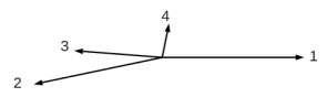
c)                                                                     d)
     
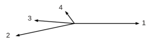
e)                                                                     f)
         

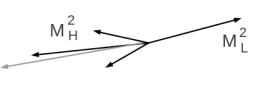
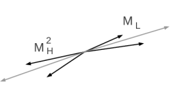
Figure 1: a) The event topologies resulting from four-jet events with requirements on the angles between the jets: $\theta_{12}>2\pi/3$, $\theta_{13}>2\pi/3$, and $\theta_{23}<\pi/6$. b) Illustration of the observable $\theta_{14}$, the angle between the first and fourth jet in the latter events. c) The event topologies resulting from four-jet events with requirements $\theta_{12}>2\pi/3$, $\theta_{13}>2\pi/3$, $\theta_{23}<\pi/6$, and $\theta_{24}<\pi/2$. d) Illustration of the observable $\theta^{*}=\theta_{24}-\theta_{23}$, the difference in opening angles. e) The sketch shows event topologies where the third and fourth clusterings occur within the same jet and hence the mass ratio $M_{L}^{2}/M_{H}^{2}$ is small. f) Events with large mass ratios, where the third and fourth clusterings occur on opposite sides of the event.

• $\theta_{14}$, proposed in Ref. [12]:
  The emission angle of the soft fourth jet with respect to the first jet; a sketch can be found in Fig. 1 b).

• $\theta^{*}$, proposed in Ref. [11]:
  A restriction on the angle between the second and fourth jet, $\theta_{24}<\pi/2$, is imposed in order to require the fourth jet to be close in angle to the nearly collinear (23) jet pair, see Fig. 1 c). The observable is the difference in opening angles, $\theta^{*}=\theta_{24}-\theta_{23}$, and is sensitive to coherent emission from the (23) jet system. A sketch of this observable is shown in Fig. 1 d).

• $C_{2}^{(1/5)}$, proposed in Ref. [17]:
  In general we have the freedom to chose the exponent $\beta$ of the 2-point energy correlation double ratio $C_{2}^{(\beta)}$. With the choice $\beta=1/5$ and a nearly collinear (23) jet pair we can express the 2-point double ratio as $C_{2}^{(1/5)}\approx E_{4}\theta_{14}^{1/5}\theta_{23\,4}^{1/5}E_{\text{vis}}/(E_{1}E_{23}\theta_{1\,23}^{1/5})$, with the total visible energy $E_{\text{vis}}$ in the event. $\theta_{23\,4}$ denotes the angle between the softest jet and the (23) jet pair and analogously for $\theta_{1\,23}$. Therefore the 2-point double ratio is mainly sensitive to the relative energy of the fourth jet.

Strong ordering in the parton shower refers to strong ordering of the clustering scales, $y^{3\to 2}\gg y^{4\to 3}\gg\ldots$, with $y^{(n+1)\to n}$ the value of the jet distance parameter in the Durham algorithm for which the configuration changes from $n+1$ to $n$ jets. In contrast, events with, e.g., $y^{4\to 3}\sim y^{3\to 2}$ are more sensitive to the ordering condition and to situations where the same parton participates in two splitting processes, hence to effective $1\to 3$ splittings. For the final observable, we cluster events into two jets and apply the restriction $y^{4\to 3}>0.5\,y^{3\to 2}$. This forces events into a compressed hierarchy, i.e., a hierarchy without strong ordering. The investigated observable is:

• $\rho=M_{L}^{2}/M_{H}^{2}$, proposed in Ref. [12]:
  The ratio of the invariant masses-squared of the jets at the end of the clustering process, ordered such that $M_{L}^{2}\leq M^{2}_{H}$. For “same-side” events, where one $1\to 3$ splitting occurs, the mass ratio is close or equal to zero, whereas for “opposite-side” events with $1\to 2\otimes 1\to 2$ splittings, the mass ratio is larger. In Fig. 1 e) and f) we illustrate examples of these event topologies. For references to heavy jet masses see, e.g. Refs. [18, 19].

To exhibit the differences between the theory models more clearly, we introduce the asymmetry for a given observable $x$,

$$\frac{N_{\text{left}}}{N_{\text{right}}}=\dfrac{\sum\limits_{i\leavevmode\nobreak\ \text{\tiny with}\leavevmode\nobreak\ x(i)<x_{0}}n_{i}}{\sum\limits_{i\leavevmode\nobreak\ \text{\tiny with}\leavevmode\nobreak\ x(i)>x_{0}}n_{i}}\leavevmode\nobreak\ ,$$ (2)

where $n_{i}$ is the number of events in histogram bin $i$ and $x(i)$ is the bin center. The dividing point $x_{0}$ separates the regions with small and large values of $x$. We use this asymmetry for three of the four observables, $\theta^{*}$, $C_{2}^{(1/5)}$, and $\rho$, and thus introduce three dividing points: $\theta^{*}_{0}$, $C_{2,0}^{(1/5)}$, and $\rho_{0}$.

As in Ref. [10], we divide the full $\theta_{14}$ range into three regions labelled “towards” (small $\theta_{14}$), “central” (intermediate $\theta_{14}$), and “away” (large $\theta_{14}$), denoted “T”, “C”, and “A” respectively. In the towards region, the first and fourth jets are collinear, while they are back-to-back in the away region. Events in which the fourth jet represents a wide-angle emission from the three-jet system populate the central region. We then consider the ratio between regions $R_{j}$ and $R_{k}$,

$$\frac{R_{j}}{R_{k}}=\dfrac{\sum\limits_{i\subset R_{j}}n_{i}}{\sum\limits_{i\subset R_{k}}n_{i}}\leavevmode\nobreak\ .$$ (3)

We define 9 different versions of the ratio, with different definitions of the regions, which are given in Table 1.

		Central/Towards	Central/Away	Towards/Away
#	Central region	Towards region	Away region	Towards region
1	$0.4<\theta_{14}/\pi<0.6$	$\theta_{14}/\pi<0.3$	$\theta_{14}/\pi>0.6$	$\theta_{14}/\pi<0.3$
2	$0.4<\theta_{14}/\pi<0.6$	$\theta_{14}/\pi<0.2$	$\theta_{14}/\pi>0.7$	$\theta_{14}/\pi<0.3$
3	$0.4<\theta_{14}/\pi<0.6$	$\theta_{14}/\pi<0.4$	$\theta_{14}/\pi>0.8$	$\theta_{14}/\pi<0.3$
4	$0.45<\theta_{14}/\pi<0.55$	$\theta_{14}/\pi<0.3$	$\theta_{14}/\pi>0.6$	$\theta_{14}/\pi<0.2$
5	$0.45<\theta_{14}/\pi<0.55$	$\theta_{14}/\pi<0.2$	$\theta_{14}/\pi>0.7$	$\theta_{14}/\pi<0.2$
6	$0.45<\theta_{14}/\pi<0.55$	$\theta_{14}/\pi<0.4$	$\theta_{14}/\pi>0.8$	$\theta_{14}/\pi<0.2$
7	$0.35<\theta_{14}/\pi<0.65$	$\theta_{14}/\pi<0.3$	$\theta_{14}/\pi>0.6$	$\theta_{14}/\pi<0.4$
8	$0.35<\theta_{14}/\pi<0.65$	$\theta_{14}/\pi<0.2$	$\theta_{14}/\pi>0.7$	$\theta_{14}/\pi<0.4$
9	$0.35<\theta_{14}/\pi<0.65$	$\theta_{14}/\pi<0.4$	$\theta_{14}/\pi>0.8$	$\theta_{14}/\pi<0.4$

Table 1: Definitions of the $\theta_{14}$ intervals used for the asymmetry ratios defined in Eq. (3). We define 9 different versions of the ratio with the labeling of the regions given in the first column. The ratio between the results in the central and towards regions is based on the definitions in columns two and three, between the central and away regions on the definitions in columns two and four, and between the towards and away regions on the definitions in columns four and five. Taken from Ref. [10].

2.2 Theory models

For parton showers based on $1\to 2$ splittings of a parton $I$ to daughters $i$ and $j$, momentum conservation requires that the virtuality of the branching parton must be compensated for by a recoil somewhere else in the event; we refer to parton $I$ as the “emitter” and to the parton (system) absorbing the recoil as the “recoiler”.

The six different theory models for the parton shower, mentioned in Section 1, are based on different formalisms and radiation functions:

• In the collinear DGLAP formalism [20, 21, 22], each parton is evolved separately and undergoes $1\to 2$ like branchings, which we denote $p_{I}\to p_{i}p_{j}$. In order to respect QCD coherence properties, a specific choice for the evolution variable [13, 23], or additional vetos [24], are applied. The momentum balancing can either include all partons of the event, which we refer to as global recoils, or only one recoiler parton, which we refer to as local recoil.

• Another formalism is based on the Catani-Seymour (CS) dipole functions [25], where a single parton emission from a pair of partons is considered. We denote the momenta involved in this splitting process with $p_{I}p_{K}\to p_{i}p_{j}p_{k}$. The full splitting probability is partitioned into two pieces, corresponding to partons $I$ and $K$, respectively, acting as the emitter with the other acting as the recoiler. The recoil is limited to the longitudinal direction of the recoiler parton in the rest frame of $I$ and $K$. If the dipole shower uses an evolution with ordering in transverse momentum, the shower correctly reproduces the soft properties of QCD.

• In the QCD antenna (also called Lund dipoles) [26, 27] picture, there is no fundamental distinction between the emitter and the recoiler. Each colour-connected parton pair of an event is represented by an antenna and undergoes a splitting process of the form $p_{I}p_{K}\to p_{i}p_{j}p_{k}$ with a $2\to 3$ recoil prescription. A single antenna thereby accounts for the equivalent of two CS dipoles.

The theory models we investigate here span all the above formalisms. For the ordering variables we use the notation $Q_{I}^{2}=(p_{i}+p_{j})^{2}$, $Q_{K}^{2}=(p_{j}+p_{k})^{2}$, and $M_{IK}^{2}=(p_{I}+p_{K})^{2}=(p_{i}+p_{j}+p_{k})^{2}$, for the splitting processes as stated above. For the DGLAP-based models, the parton $K$ acts as the recoiler and can either represent a single parton (Pythia 8) or multiple partons (Herwig++).

In the following we briefly describe the main differences between the theory models used in this paper, mostly concentrated on the aspects described above. Herwig++ $\tilde{q}^{2}$ [13], a parton shower model based on DGLAP splitting kernels, uses global recoils. The evolution is ordered in a variable proportional to energy times angle,

$$\tilde{q}^{2} =\frac{Q_{I}^{2}M_{IK}^{4}}{Q_{K}^{2}(M_{IK}^{2}-Q_{I}^{2}-Q_{K}^{2})}\leavevmode\nobreak\ .$$ (4)

The shower includes a matrix-element correction for the first emission and uses two-loop running of $\alpha_{s}$. The QCD coherence properties are respected due to the angular ordering of the parton branching cascade. The second shower model in the Herwig++ event generator is Herwig++ $p_{\perp\mathrm{dip}}^{2}$ [11], which is based on partitioned CS dipoles with local recoils within dipoles. The ordering variable is the relative transverse momentum of the splitting pair,

$$p^{2}_{\perp\mathrm{dip}} =\frac{Q_{I}^{2}Q_{K}^{2}(M_{IK}^{2}-Q_{I}^{2}-Q_{K}^{2})}{(M_{IK}^{2}-Q_{I}^{2})^{2}}\leavevmode\nobreak\ .$$ (5)

We do not apply matching or matrix-element corrections and use one-loop running of $\alpha_{s}$. The dipole shower with ordering in transverse momentum respects QCD coherence. As an alternative we use the same shower model, but with a different ordering variable. Herwig++ $q_{\mathrm{dip}}^{2}$ [11] orders the shower cascade in virtuality of the splitting pair,

$$q_{\mathrm{dip}}^{2} =Q_{I}^{2}\leavevmode\nobreak\ .$$ (6)

As before we do not apply matching or matrix-element corrections and use one-loop running of $\alpha_{s}$. Vincia $p_{\perp\mathrm{ant}}^{2}$ [15] is a shower model based on antenna functions with local recoils within antennae. The ordering variable is the transverse momentum of the antenna,

$$p_{\perp\mathrm{ant}}^{2} =\frac{Q^{2}_{I}Q^{2}_{K}}{M_{IK}^{2}}\leavevmode\nobreak\ .$$ (7)

Matrix-element corrections at LO [28] and NLO [29] are switched off and we use one-loop running of $\alpha_{s}$. Colour coherence is respected, since it is an intrinsic property of the antenna functions. Transverse momentum as the evolution variable is the preferred choice in Vincia, as has been shown in Ref. [29]. However, we also use Vincia $m_{\mathrm{ant}}^{2}$ [15] as an alternative to the transverse momentum ordering, which orders the shower evolution in antenna mass, defined as

$$m_{\mathrm{ant}}^{2} =\min(Q^{2}_{I},Q^{2}_{K})\leavevmode\nobreak\ .$$ (8)

The last shower model is Pythia 8 $p_{\perp\mathrm{evol}}^{2}$ [14], a parton shower based on DGLAP splitting kernels and ordered in transverse momentum, defined as

$$p^{2}_{\perp\mathrm{evol}} =\frac{Q_{I}^{2}(M^{2}_{IK}-Q^{2}_{K})(Q^{2}_{I}+Q^{2}_{K})}{(M^{2}_{IK}+Q^{2}_{I})^{2}}\leavevmode\nobreak\ .$$ (9)

In contrast to the angular ordered Herwig++ shower, local recoils within dipoles are applied. A matrix-element correction for the first emission is included and we use one-loop running of $\alpha_{s}$. To obtain QCD coherence properties, the shower applies angular vetoes.

Besides the shower models used in this paper, there are several other models: Ariadne  [30], based on antenna functions, which is very similar to Vincia; the CS dipole shower models of Weinzierl et al. [31], and Sherpa [32], which are similar to the Herwig++ dipole shower; the deductor by Nagy and Soper [33], which is not interfaced with a hadronization model; and the virtuality-ordered final-state showers of Pythia  [24, 34], Nlljet [35] and Herwiri [36].

To compare the models on as equal a footing as possible, the shower and hadronization parameters have been readjusted with the Professor [37] tuning system, utilizing LEP data available through Rivet [38]. The tuning procedure is described in Ref. [10], where the resulting parameter values can also be found.

3 OPAL experiment

The OPAL experiment at LEP operated between August 1989 and November 2000. The detector components were arranged around the beam pipe, in a layered structure. A detailed description can be found in Refs. [39, 40, 41]. The tracking system consisted of a silicon microvertex detector, an inner vertex chamber, a jet chamber, and chambers outside the jet chambers to improve the precision of the $z$-coordinate measurement. The jet chamber was approximately $4\leavevmode\nobreak\ \mathrm{m}$ long and had an outer radius of about $1.85\leavevmode\nobreak\ \mathrm{m}$. This device had $24$ sectors each containing $159$ sense wires spaced by 1 cm. All tracking systems were located inside a solenoidal magnet, which provided a uniform axial magnetic field of $0.435\leavevmode\nobreak\ \mathrm{T}$ along the beam axis. The magnet was surrounded by a lead glass electromagnetic calorimeter and a sampling hadron calorimeter. The electromagnetic calorimeter consisted of $11704$ lead glass blocks, divided into barrel and endcap sections, covering $98\%$ of the solid angle. Outside the hadron calorimeter, the detector was surrounded by a system of muon chambers. Similar layers of instrumentation were located in the endcap regions.

Since the energy resolution of the electromagnetic calorimeter is better then that of the hadron calorimeter, the resolution of jet directions and energies is not significantly improved by incorporating hadron calorimeter information. Thus, our analysis relies exclusively on charged particle information recorded in the tracking detectors and on clusters of energy deposited in the electromagnetic calorimeter.

4 Data and MC samples

In the first phase of LEP operation, denoted LEP1 (1989 to 1995), the $e^{+}e^{-}$ center-of-mass energy was chosen to lie at or near the mass of the $Z$ boson, $\sqrt{s}\approx 91\leavevmode\nobreak\ \mathrm{GeV}$. During the second phase of operation, denoted LEP2 (1995-2000), the center-of-mass energy was increased in successive steps from $130$ to $209\leavevmode\nobreak\ \mathrm{GeV}$. Interspersed at various times during the LEP2 operation, calibration runs were collected at the $Z$ boson peak. In this analysis, we utilize data collected at $\sqrt{s}=91.2$ GeV during the the LEP2 calibration runs. This allows us to exploit conditions when the detector was operating in its final, most advanced configuration. In addition, this will facilitate possible future comparisons with data collected under essentially identical conditions at higher energies. We use a sample corresponding to an integrated luminosity of $14.7\leavevmode\nobreak\ \mathrm{pb}^{-1}$. This sample is of sufficient size that systematic uncertainties dominate the statistical terms. To correct the data in order to account for experimental acceptance and efficiency, simulated event samples produced with MC event generators are used. The process $e^{+}e^{-}\to q\bar{q}$ is simulated using Pythia 6.1 [42] at $\sqrt{s}=91.2$ GeV. Corresponding samples using Herwig 6.2 [43, 44] are used for systematic checks. We examine the MC events at two levels. We refer to “hadron level” as events without event selection, and without simulation of the detector acceptance and resolution, for which all particles with lifetimes less than $300\leavevmode\nobreak\ \mathrm{ps}$ decay. In contrast, “detector level” refers to MC events that are processed through the Geant4-based [45] simulation of the OPAL detector, called Gopal [46], and that have been reconstructed using the same software procedures that are applied to the data. The MC events generated for the detector-level samples are the same as the hadron-level samples except that $K^{0}_{S}$ mesons and weakly decaying hyperons are declared to be stable, as these particles can interact with detector material before decaying, and so their decays are handled within the Geant framework.

In addition, for comparisons with the corrected data, large samples of hadron-level MC events are employed, using the event generators Herwig++ 2.7.0 [47], Pythia 8.176 [48], and Vincia 1.1.0 [15] interfaced with the hadronization model of Pythia 8.176.

5 Data analysis

5.1 Selection of events

The same criteria for the selection of charged tracks and electromagnetic clusters are applied as described in Ref. [49]. Charged tracks are required to have transverse momentum relative to the beam axis larger than $0.15\leavevmode\nobreak\ \mathrm{GeV}$, and photons to have energies larger than $0.10\leavevmode\nobreak\ \mathrm{GeV}$ ($0.25\leavevmode\nobreak\ \mathrm{GeV}$) in the barrel (endcap) region of the electromagnetic calorimeter. The selection of hadronic annihilation events is the same as described in Ref. [50]. Briefly, a minimum of five charged tracks is required, and a containment condition $|\cos\theta_{\mathrm{T}}|<0.90$ is applied, where $\theta_{\rm{T}}$ is the polar angle of the thrust axis [51, 52] with respect to the beam axis, calculated using all accepted charged tracks and electromagnetic clusters. A total of $397\,452$ candidate hadronic annihilation events are selected, with a negligible expected background.

Since the energy loss due to initial-state radiation is highly suppressed at the $Z$ peak, we do not apply a cut to that effect. However, radiative corrections are applied by requiring $\sqrt{s}-\sqrt{s^{\prime}}<1\leavevmode\nobreak\ \mathrm{GeV}$ for the MC detector-level samples used to correct the data, where $\sqrt{s^{\prime}}$ is the effective center-of-mass energy after initial-state radiation.

5.2 Reconstruction and correction

For each of the accepted events, the values of all observables described in Section 1 are computed. To avoid double-counting of energy between tracks and electromagnetic clusters, an energy-flow algorithm [53, 54] is applied, which matches the tracks and clusters and retains only those clusters that are not associated with a track.

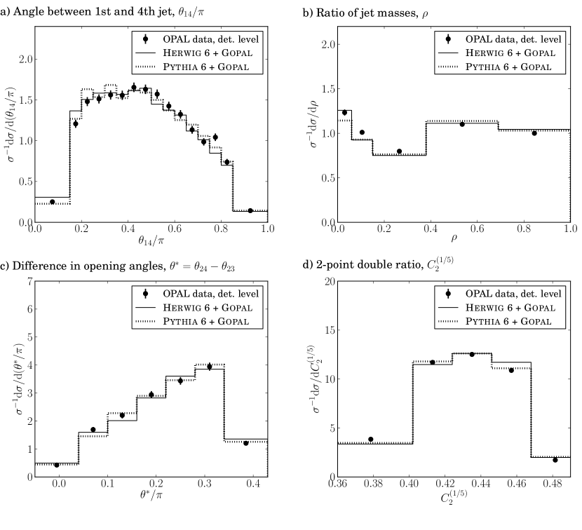
Figure 2: The uncorrected distributions of a) the emission angle $\theta_{14}$, b) the mass ratio $\rho=M_{L}^{2}/M_{H}^{2}$, c) the difference in opening angles $\theta^{*}$, and d) the 2-point double ratio $C_{2}^{(1/5)}$, in comparison with the predictions of the Herwig 6 and Pythia 6 Monte Carlo event generators at the detector level. The error bars indicate the statistical uncertainties.

Figure 2 shows a comparison of the uncorrected data with the detector-level predictions of Pythia 6 and Herwig 6 for the $\theta_{14}$, $\rho$, $\theta^{*}$, and $C_{2}^{(1/5)}$ variables. The $\theta_{14}$ and $\theta^{*}$ variables are normalized by a factor of $\pi$. The simulations are seen to provide a generally adequate description of the measurements.

To correct the data for detector and resolution effects, we implement an unfolding procedure based on the RooUnfold [55] framework. We use the iterative Bayes method, as proposed by D’Agostini [56], with four iterations, which is the recommendation from Ref. [55]. A necessary ingredient for the unfolding is the response matrix of the MC event generator used for the correction procedure. For the standard analysis, Pythia 6 is used to determine the response matrix. The response matrix gives the bin-to-bin migration from the hadron to the detector level, and vice versa. In order to obtain reliable results for the corrected distributions, we adjust the bin widths of the histograms such that the probability for a hadron-level event to migrate to a different bin at the detector level is less than $50\%$.

The corrected distributions are presented in Fig. 3 and Tables LABEL:tab:dataBinNorm1-LABEL:tab:dataBinNorm2. Tables LABEL:tab:dataBinNorm1-LABEL:tab:dataBinNorm2 include the covariance matrices calculated with RooUnfold. The statistical uncertainties are given by the square root of the corresponding diagonal element in the covariance matrices. Systematic uncertainties are discussed in Section 5.3. Figure 3 includes the predictions of Pythia 6 and Herwig 6 at the hadron level. The differences between the MC predictions and the data are seen to be similar to those observed at the detector level (Fig. 2), demonstrating that the correction procedure does not introduce a discernible bias.

The values of the derived distributions, i.e., the ratios of the different regions for $\theta_{14}$ and the asymmetry for the other observables, are listed in Table LABEL:tab:dataAS. The quantities are determined by summing and dividing the histogram entries. The statistical uncertainties are evaluated from propagation of errors, while the systematic uncertainties are determined as described in Section 5.3.

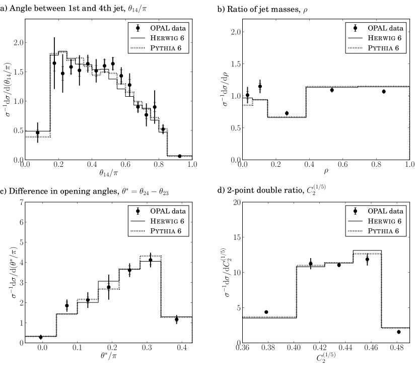
Figure 3: The corrected distributions of a) the emission angle $\theta_{14}$, b) the mass ratio $\rho=M_{L}^{2}/M_{H}^{2}$, c) the difference in opening angles $\theta^{*}$, and d) the 2-point double ratio $C_{2}^{(1/5)}$, in comparison with the predictions of the Herwig 6 and Pythia 6 Monte Carlo event generators at the hadron level. The error bars limited by the horizontal lines indicate the statistical uncertainties, while the total uncertainties correspond to the full error bars.

5.3 Systematic uncertainties

Systematic uncertainties are evaluated by repeating the analysis with different selection requirements and with variations in the correction procedure. Specifically, we consider the following:

• The requirement on the thrust angle direction is changed to $|\cos\theta_{\mathrm{T}}|<0.7$ from the default $|\cos\theta_{\mathrm{T}}|<0.9$.

• The minimum number of charged tracks is increased to seven from the default of five.

• Variation of the reconstruction procedure: All tracks and clusters are taken into account. In this case the detector correction takes care of the double counting.

• Herwig 6 is used in place of Pythia 6 to determine the response matrix.

The systematic uncertainty is determined for each variation from the bin-by-bin difference in the corrected distributions with respect to the standard result. The total systematic uncertainty is given by the quadrature sum of the individual terms. The total uncertainty of the data is defined by summing the statistical and systematic contributions in quadrature.

As additional systematic checks on the unfolding procedure, we consider the following variations:

• We use the unfolding method with three and five instead of four iterations.

• Instead of the iterative method, we use the singular value decomposition, as proposed by Höcker and Kartvelishvili [57] and implemented in RooUnfold.

We find the systematic variations that arise from these two checks to be smaller or comparable to the variation observed when using Herwig 6 in place of Pythia 6. Since adding all these effects together would likely double count the uncertainty associated with the unfolding procedure we do not add the observed differences to the systematic uncertainty.

6 Comparison with Monte Carlo models

In this section, we present a comparison between the coherence schemes described in Section 2.2 and the data. For this purpose, samples of $5\times 10^{6}$ events are generated for each MC model, using the tuned parameter sets mentioned in Section 2.2. We present the predictions for the different schemes in terms of the observables defined in Section 1. As a measure of the level of agreement with data, we calculate the significance, defined as

$$\sigma_{i}=\frac{\text{MC}_{i}-\mathcal{D}_{i}}{\sigma_{\mathcal{D}_{i}}}\leavevmode\nobreak\ ,$$ (10)

where $\text{MC}_{i}$ and $\mathcal{D}_{i}$ represent the predicted and observed values in bin $i$ of a distribution, with $\sigma_{\mathcal{D}_{i}}$ the corresponding uncertainty in $\mathcal{D}_{i}$. In the following, we present a distribution of the significance in a plot below the distribution of the variables. In addition we calculate the $\chi^{2}$ values for the distribution as

$$\chi^{2}=(\text{MC}-\mathcal{D})^{\text{T}}V^{-1}(\text{MC}-\mathcal{D})=\sum_{i,j=1}^{N_{\mathrm{bins}}}(\text{MC}-\mathcal{D})_{i}(V^{-1})_{ij}(\text{MC}-\mathcal{D})_{j}\leavevmode\nobreak\ ,$$ (11)

where $V$ is the full covariance matrix, representing statistical terms, with systematic uncertainties added to the diagonal elements. We present the $\chi^{2}$ results and corresponding p-values in Table LABEL:tab:chi2values. The latter are calculated with the Root [58] program and give the probability that the deviations of the MC predictions from the data are consistent with the evaluated uncertainties.

6.1 Angle between first and fourth jet: $\theta_{14}$

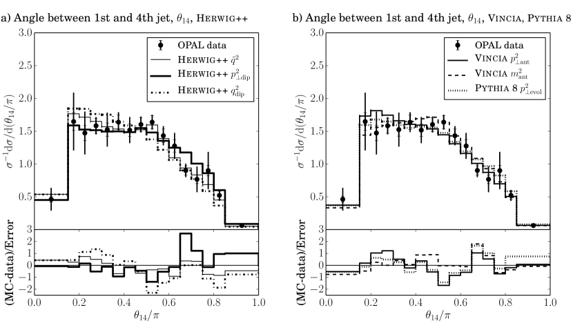
Figure 4: The corrected distribution of the emission angle $\theta_{14}$ of the soft fourth jet in comparison with the predictions of a) Herwig++ and b) Pythia 8 and Vincia. The thin solid lines correspond to Herwig++ with angular-ordering ($\tilde{q}^{2}$), the thick solid lines to the dipole shower of Herwig++ with ordering in $p_{\perp\mathrm{dip}}^{2}$, and the dash-dotted lines to ordering in $q_{\mathrm{dip}}^{2}$. Vincia with ordering in $p_{\perp\mathrm{ant}}^{2}$ is shown with medium solid lines, ordering in $m_{\mathrm{ant}}^{2}$ with dashed lines, and Pythia 8 is shown with dotted lines. The error bars limited by the horizontal lines indicate the statistical uncertainties, while the total uncertainties correspond to the full error bars. The ratio plots show the deviation of the predictions from the data in units of the total uncertainty.

In Figs. 4 a) and b) we show the normalized distribution of the emission angle of the soft fourth jet from the nearly collinear three-jet system, $\theta_{14}$. All models are found to provide adequate descriptions of the data, except that the Herwig++ $p_{\perp\mathrm{dip}}^{2}$ model lies about three standard deviations above the measurements for a narrow region around $\theta_{14}\approx 0.7\pi$. Even for this model, the p-value is $0.42$ (Table LABEL:tab:chi2values), implying overall compatibility with the experimental results.

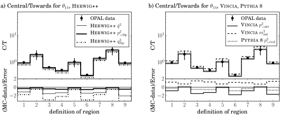
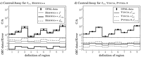
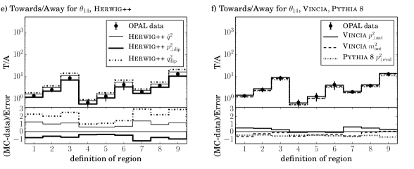
Figure 5: The corrected data for the derived distributions in comparison with the predictions of a) Herwig++ and b) Pythia 8 and Vincia. The thin solid lines correspond to Herwig++ with angular-ordering ($\tilde{q}^{2}$), the thick solid lines to the dipole shower of Herwig++ with ordering in $p_{\perp\mathrm{dip}}^{2}$, and the dash-dotted lines to ordering in $q_{\mathrm{dip}}^{2}$. Vincia with ordering in $p_{\perp\mathrm{ant}}^{2}$ is shown with medium solid lines, ordering in $m_{\mathrm{ant}}^{2}$ with dashed lines, and Pythia 8 is shown with dotted lines. The error bars limited by the horizontal lines indicate the statistical uncertainties, while the total uncertainties correspond to the full error bars. The ratio plots show the deviation of the predictions from the data in units of the total uncertainty.

We show the ratio C/T of the central-to-towards regions, which gives the relative amount of wide-angle to collinear emissions, in Figs. 5 a) and b). For the $p_{\perp\mathrm{dip}}^{2}$-ordered dipole shower of Herwig++ and the parton shower of Pythia 8 we find nearly perfect agreement with the data for all nine C/T regions (Table 1). The Herwig++ $\tilde{q}^{2}$ model and the Vincia $p^{2}_{\perp\mathrm{ant}}$ model lie below the data by up to two standard deviations in some regions, while the Vincia $m^{2}_{\mathrm{ant}}$ model lies about two standard deviations above the data in all regions. The two Vincia models exhibit the expected behavior: When the antenna mass is used as the evolution variable, soft wide-angle emissions are preferred over collinear ones, which leads to higher values for the relative level of wide-angle to collinear emissions. This demonstrates the sensitivity of the $\theta_{14}$ variable to the choice of evolution scheme. The largest deviation from the data in Figs. 5 a) and b) is observed for the $q_{\mathrm{dip}}^{2}$-ordered dipole shower of Herwig++, for which the predictions lie up to around three standard deviations below the data in some regions. Thus, this model predicts too many collinear emissions compared to wide-angle emissions.

In Figs. 5 c) and d) we show a comparison of the MC predictions to the data for the ratio C/A of the central-to-away regions. This ratio measures the relative amount of wide-angle emissions to emissions in a backwards direction, away from the leading jet and near to the collinear (23) jet pair. For the Herwig++ $\tilde{q}^{2}$ model and for Vincia, we find a good agreement with the data and observe small differences for the different evolution variables of Vincia. Pythia 8 and the $p_{\perp\mathrm{dip}}^{2}$-ordered dipole shower of Herwig++ lie below the data, by around one and two standard deviations, respectively, and thus predict too few wide-angle emissions compared to the backwards emissions. The Herwig++ $q_{\mathrm{dip}}^{2}$ model lies around one standard deviation above the data and thus predicts relatively too many wide-angle emissions. The observations the ratios C/T and C/A are confirmed by the measurements of the ratio T/A of the towards-to-away regions, presented in Figs. 5 e) and f).

6.2 Difference in opening angles: $\theta^{*}$

In Figs. 6 a) and b) we show the normalized distribution of the difference in opening angles between the third and the fourth jet with respect to the second jet, $\theta^{*}=\theta_{24}-\theta_{23}$. All models are seen to provide an adequate description of the data, with the exception of the region around $\theta^{*}\approx 0.07\pi$ (second bin of Figs. 6 a) and b)), where the models predict somewhat fewer events than are observed. The largest discrepancy in this region arises from the Herwig++ $q_{\mathrm{dip}}^{2}$ model.

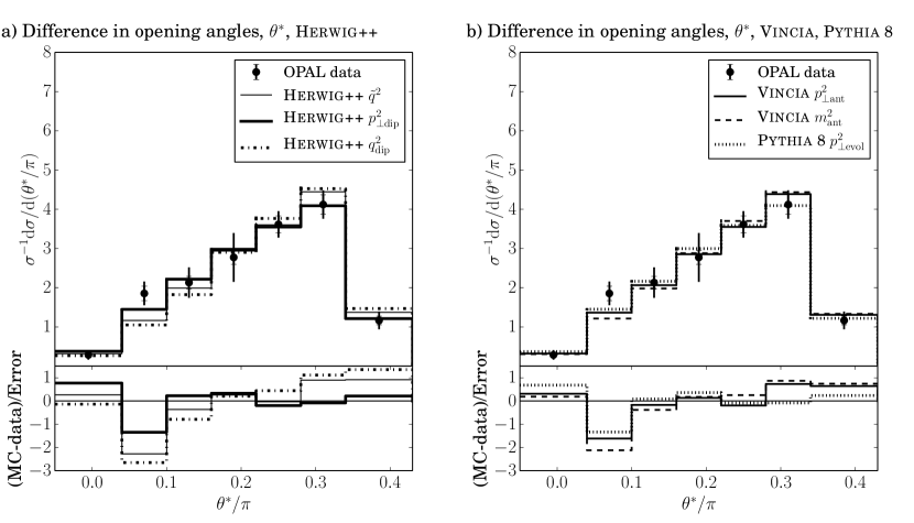
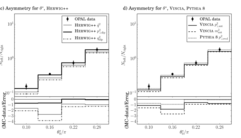
Figure 6: The distribution of the difference in opening angles $\theta^{*}$ for a) Herwig++ and b) Pythia 8 and Vincia. The asymmetry with respect to the dividing point $\theta^{*}_{0}$ is shown for c) Herwig++ and d) Pythia 8 and Vincia. The thin solid lines correspond to Herwig++ with angular-ordering ($\tilde{q}^{2}$), the thick solid lines to the dipole shower of Herwig++ with ordering in $p_{\perp\mathrm{dip}}^{2}$, and the dash-dotted lines to ordering in $q_{\mathrm{dip}}^{2}$. Vincia with ordering in $p_{\perp\mathrm{ant}}^{2}$ is shown with medium solid lines, ordering in $m_{\mathrm{ant}}^{2}$ with dashed lines and Pythia 8 is shown with dotted lines. The error bars limited by the horizontal lines indicate the statistical uncertainties, while the total uncertainties correspond to the full error bars. The ratio plots show the deviation of the predictions from the data in units of the total uncertainty.

We show the asymmetry as a function of the dividing point $\theta^{*}_{0}$ in the Figs. 6 c) and d). The largest discriminating power is found for $\theta_{0}*=0.16\pi$, where the $q_{\mathrm{dip}}^{2}$-ordered dipole shower of Herwig++ generates a deviation of almost four standard deviations with respect to the data. The number of events with large differences in the opening angles of the third and fourth jets is overestimated by this non-coherent shower model. The $p^{2}_{\perp\mathrm{dip}}$-ordered Herwig++ shower, based on the same shower kernels, but respecting coherence due to the choice of evolution variable, gives a better description of the asymmetry. This emphasizes the need for coherence in order to describe the data properly.

6.3 2-Point double ratio: $C_{2}^{(1/5)}$

For the normalized distribution of the 2-point double ratio, $C_{2}^{(1/5)}$, shown in Figs. 7 a) and b), we find rather large deviations between the data and the MC prediction for most of the shower models. We again find that the $q_{\mathrm{dip}}^{2}$-ordered Herwig++ shower exhibits the largest discrepancies. Only two models, Pythia 8 and the Vincia $m_{\mathrm{ant}}^{2}$ model, yield p-values larger than $50\%$ (Table LABEL:tab:chi2values).

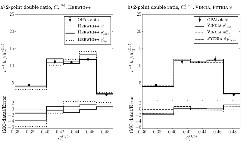
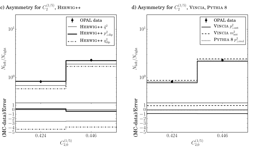
Figure 7: The distribution of the difference in opening angles $C_{2}^{(1/5)}$ for a) Herwig++ and b) Pythia 8 and Vincia. The asymmetry with respect to the dividing point $C_{2,0}^{(1/5)}$ is shown for c) Herwig++ and d) Pythia 8 and Vincia. The thin solid lines correspond to Herwig++ with angular-ordering ($\tilde{q}^{2}$), the thick solid lines to the dipole shower of Herwig++ with ordering in $p_{\perp\mathrm{dip}}^{2}$, and the dash-dotted lines to ordering in $q_{\mathrm{dip}}^{2}$. Vincia with ordering in $p_{\perp\mathrm{ant}}^{2}$ is shown with medium solid lines, ordering in $m_{\mathrm{ant}}^{2}$ with dashed lines and Pythia 8 is shown with dotted lines. The error bars limited by the horizontal lines indicate the statistical uncertainties, while the total uncertainties correspond to the full error bars. The ratio plots show the deviation of the predictions from the data in units of the total uncertainty.

In Figs. 7 c) and d), we show the asymmetry in the $C_{2}^{(1/5)}$ variable as a function of the dividing point $C_{2,0}^{(1/5)}$. Since $C_{2}^{(1/5)}$ is proportional to the energy $E_{4}$ of the fourth jet, the asymmetry in $C_{2}^{(1/5)}$ measures the relative number of events of soft versus hard fourth-jet emissions. We observe large deviations from the data, at the level of four standard deviations, for the Herwig++ $q_{\mathrm{dip}}^{2}$ model, which underpredicts the relative fraction of events with a very soft fourth jet. A similar discrepancy, at the level of around $2.5$ standard deviations, is observed for the Herwig++ $\tilde{q}^{2}$ model. The two versions of Vincia exhibit deviations of about one standard deviation in the opposite sense, i.e., Vincia $m_{\mathrm{ant}}^{2}$ somewhat overpredicts the level of hard fourth-jet emissions, whereas Vincia $p_{\perp\mathrm{ant}}^{2}$ predicts too few hard fourth-jet emissions. In contrast, the Herwig++ $p_{\perp\mathrm{dip}}^{2}$ and Pythia 8 models are in nearly perfect agreement with the data.

6.4 Mass ratio: $\rho=M_{L}^{2}/M_{H}^{2}$

The normalized distributions of the $\rho=M_{L}^{2}/M_{H}^{2}$ variable are shown in Figs. 8 a) and b). For the Pythia 8 and the two Vincia models, we find reasonable overall agreement with the data, with differences on the level of two standard deviations or less. The Herwig++ models demonstrate larger differences, with discrepancies reaching the level of four standard deviations for the Herwig++ $q_{\mathrm{dip}}^{2}$ model.

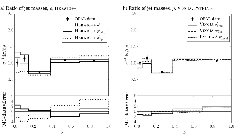
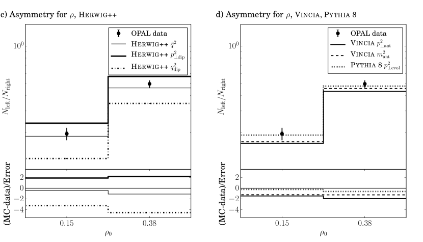
Figure 8: The distribution of the difference in opening angles $\rho=M_{L}^{2}/M_{H}^{2}$ for a) Herwig++ and b) Pythia 8 and Vincia. The asymmetry with respect to the dividing point $\rho_{0}$ is shown for c) Herwig++ and d) Pythia 8 and Vincia. The thin solid lines correspond to Herwig++ with angular-ordering ($\tilde{q}^{2}$), the thick solid lines to the dipole shower of Herwig++ with ordering in $p_{\perp\mathrm{dip}}^{2}$, and the dash-dotted lines to ordering in $q_{\mathrm{dip}}^{2}$. Vincia with ordering in $p_{\perp\mathrm{ant}}^{2}$ is shown with medium solid lines, ordering in $m_{\mathrm{ant}}^{2}$ with dashed lines and Pythia 8 is shown with dotted lines. The error bars limited by the horizontal lines indicate the statistical uncertainties, while the total uncertainties correspond to the full error bars. The ratio plots show the deviation of the predictions from the data in units of the total uncertainty.

In Figs. 8 c) and d) we show the asymmetry of the $\rho$ variable as a function of the dividing point $\rho_{0}$. This asymmetry is sensitive to the relative number of same-side versus opposite-side events, whose definitions were given in Section 2.1. This asymmetry is seen to provide discrimination between most of the shower models. The Pythia 8 and Herwig++ $\tilde{q}^{2}$ models yield predictions that lie within one standard deviation of the data. However, the Herwig++ $q_{\mathrm{dip}}^{2}$ model predicts too small an asymmetry by about four standard deviations, meaning that there are too few same-side compared to opposite-side events. The two Vincia models also predict too few same-side events, but only at the level of around one standard deviation. In contrast, the Herwig++ $p_{\perp\mathrm{dip}}^{2}$ model predicts relatively too many same-side events, at the level of two standard deviations.

7 Summary and conclusion

We have presented measurements of distributions in $e^{+}e^{-}$ annihilations at $\sqrt{s}=91.2\leavevmode\nobreak\ \mathrm{GeV}$ that are sensitive to QCD colour coherence, the ordering parameter in parton showers, and to whether four-jet events arise from two separate $1\to 2$ splittings or from a $1\to 3$ splitting. The data, corresponding to a sample of about $397\leavevmode\nobreak\ 000$ hadronic annihilation events, were collected with the OPAL detector at LEP. The event selection criteria are defined in a way to minimize the influence of non-perturbative (hadronization) effects. We compared the data with six different models for the parton shower, based on the Herwig++, Pythia 8, and Vincia Monte Carlo event generator programs, which differ in the choice of the radiation function, ordering variable, and recoil strategy. Each of the six models was found to be in general agreement with the data. However, interesting differences between the models and between some of the models and the data were observed when asymmetries in the distributions were examined.

Until now it was nearly impossible to distinguish between the predictions of Pythia 8 and Vincia, or between the different variants of Vincia. Our study of the asymmetry of the ratio of squared jet masses, shown in Fig. 8 d), shows that Vincia predicts somewhat too many opposite-side events (i.e., events with two $1\to 2$ splittings) compared to same-side events (i.e., events with a $1\to 3$ splitting), and that the data prefer Pythia 8. We find that the different variants of Vincia can be distinguished using the central-to-towards (Fig. 5 b)) and central-to-away (Fig. 5 d)) ratios in the $\theta_{14}$ variable, which indicate that the Vincia variant based on antenna mass-squared evolution predicts somewhat too many wide-angle emissions for the soft fourth jet, compared to collinear emissions.

To summarize the results of our study, we show the average p-value for each model, calculated from the four values of the single observables, in the bottom row of Table LABEL:tab:chi2values. The variant of Herwig++ with a $q^{2}_{\mathrm{dip}}$-ordered dipole shower is found to provide the least satisfactory description of the data. This model does not contain coherence; it has intentionally been introduced to confront it with coherent evolution. Thus our results emphasize the importance of incorporating coherence into the description of the QCD multijet process. Since Herwig++ uses the cluster [23] and Pythia 8 and Vincia use the Lund string [59, 60] hadronization model, a direct comparison of the predictions from the two groups of shower models is somewhat ambiguous. It would be interesting to perform a comparison based on use of the same hadronization model for all models. However, when comparing all shower models together, we find Pythia 8 and Vincia with evolution in transverse momentum to give the best description of the measurements presented here.

Acknowledgements

We would like to express our gratitude to the members of the editorial board (S. Bentvelssen, S. Bethke, J.W. Gary, K. Rabbertz) for their careful review of the analysis and the draft resulting in this publication.

NF would like to thank CERN for hospitality during the course of this work. This work was supported by the FP7 Marie Curie Initial Training Network MCnetITN under contract number PITN-GA-2012-315877. SG and SP acknowledge support from the Helmholtz Alliance “Physics at the Terascale”. SP acknoweldges support through a Marie Curie Intra-European Fellowship under contract number PIEF-GA-2013-628739.

We particularly wish to thank the SL Division for the efficient operation of the LEP accelerator at all energies and for their close cooperation with our experimental group. In addition to the support staff at our own institutions we are pleased to acknowledge the Department of Energy, USA,
National Science Foundation, USA,
Particle Physics and Astronomy Research Council, UK,
Natural Sciences and Engineering Research Council, Canada,
Israel Science Foundation, administered by the Israel Academy of Science and Humanities,
Benoziyo Center for High Energy Physics,
Japanese Ministry of Education, Culture, Sports, Science and Technology (MEXT) and a grant under the MEXT International Science Research Program,
Japanese Society for the Promotion of Science (JSPS),
German Israeli Bi-national Science Foundation (GIF),
Bundesministerium für Bildung und Forschung, Germany,
National Research Council of Canada,
Hungarian Foundation for Scientific Research, OTKA T-038240, and T-042864,
The NWO/NATO Fund for Scientific Research, the Netherlands.

References

- [1] For the author list of the OPAL collaboration refer to G. Abbiendi et al., Eur. Phys. J. C 71 (2011) 1733.
- [2] MCnet Collaboration, A. Buckley et al., Phys. Rept. 504 (2011) 145.
- [3] J. Beringer et al. (Particle Data Group), Phys. Rev. D 86 (2012) 010001.
- [4] M. H. Seymour and M. Marx, arXiv:1304.6677 [hep-ph].
- [5] S. Gieseke, Prog. Part. Nucl. Phys. 72 (2013) 155.
- [6] OPAL Collaboration, G. Abbiendi et al., Phys. Lett. B 638 (2006) 30, arXiv:hep-ex/0604003 [hep-ex].
- [7] DELPHI Collaboration, J. Abdallah et al., Phys. Lett. B 605 (2005) 37, arXiv:hep-ex/0410075 [hep-ex].
- [8] A. H. Mueller, Phys. Lett. B 104 (1981) 161.
- [9] Y. L. Dokshitzer, V. S. Fadin, and V. A. Khoze, Phys. Lett. B 115 (1982) 242.
- [10] N. Fischer, S. Gieseke, S. Plätzer, and P. Z. Skands, Eur. Phys. J. C 74 (2014) 2831, arXiv:1402.3186 [hep-ph].
- [11] S. Plätzer and S. Gieseke, JHEP 1101 (2011) 024, arXiv:0909.5593 [hep-ph].
- [12] J. Alcaraz Maestre et al., arXiv:1203.6803 [hep-ph].
- [13] S. Gieseke, P. Stephens, and B. Webber, JHEP 0312 (2003) 045, arXiv:hep-ph/0310083 [hep-ph].
- [14] T. Sjöstrand and P. Z. Skands, Eur. Phys. J. C 39 (2005) 129, arXiv:hep-ph/0408302 [hep-ph].
- [15] W. T. Giele, D. A. Kosower, and P. Z. Skands, Phys. Rev. D 78 (2008) 014026, arXiv:0707.3652 [hep-ph].
- [16] S. Catani, Y. L. Dokshitzer, M. Olsson, G. Turnock, and B. Webber, Phys. Lett. B 269 (1991) 432.
- [17] A. J. Larkoski, G. P. Salam, and J. Thaler, JHEP 1306 (2013) 108, arXiv:1305.0007 [hep-ph].
- [18] T. Chandramohan and L. Clavelli, Nucl. Phys. B 184 (1981) 365.
- [19] L. Clavelli and D. Wyler, Phys. Lett. B 103 (1981) 383.
- [20] V. N. Gribov and L. N. Lipatov, Sov. J. Nucl. Phys. 15 (1972) 438.
- [21] G. Altarelli and G. Parisi, Nucl. Phys. B 126 (1977) 298.
- [22] Y. L. Dokshitzer, Sov. Phys. JETP 46 (1977) 641.
- [23] G. Marchesini and B. Webber, Nucl. Phys. B 238 (1984) 1.
- [24] M. Bengtsson and T. Sjöstrand, Nucl. Phys. B 289 (1987) 810.
- [25] S. Catani and M. H. Seymour, Nucl. Phys. B 485 (1997) 291, arXiv:hep-ph/9605323 [hep-ph].
- [26] G. Gustafson and U. Pettersson, Nucl. Phys. B 306 (1988) 746.
- [27] D. A. Kosower, Phys. Rev. D 71 (2005) 045016, arXiv:hep-ph/0311272 [hep-ph].
- [28] W. T. Giele, D. A. Kosower, and P. Z. Skands, Phys. Rev. D 84 (2011) 054003, arXiv:1102.2126 [hep-ph].
- [29] L. Hartgring, E. Laenen, and P. Z. Skands, JHEP 1310 (2013) 127, arXiv:1303.4974 [hep-ph].
- [30] L. Lönnblad, Comput. Phys. Commun. 71 (1992) 15.
- [31] M. Dinsdale, M. Ternick, and S. Weinzierl, Phys. Rev. D 76 (2007) 094003, arXiv:0709.1026 [hep-ph].
- [32] S. Schumann and F. Krauss, JHEP 0803 (2008) 038, arXiv:0709.1027 [hep-ph].
- [33] Z. Nagy and D. E. Soper, JHEP 1406 (2014) 097, arXiv:1401.6364 [hep-ph].
- [34] M. Bengtsson and T. Sjöstrand, Phys. Lett. B 185 (1987) 435.
- [35] K. Kato and T. Munehisa, Comput. Phys. Commun. 64 (1991) 67.
- [36] B. F. L. Ward, S. Joseph, S. Majhi, and S. A. Yost, PoS RADCOR2009 (2010) 070, arXiv:1001.2730 [hep-ph].
- [37] A. Buckley, H. Hoeth, H. Lacker, H. Schulz, and J. E. von Seggern, Eur. Phys. J. C 65 (2010) 331, arXiv:0907.2973 [hep-ph].
- [38] A. Buckley et al., Comput. Phys. Commun. 184 (2013) 2803, arXiv:1003.0694 [hep-ph].
- [39] OPAL Collaboration, K. Ahmet et al., Nucl. Instrum. Meth. A 305 (1991) 275.
- [40] OPAL Collaboration, S. Anderson et al., Nucl. Instrum. Meth. A 403 (1998) 326.
- [41] G. Aguillion et al., Nucl. Instrum. Meth. A 417 (1998) 266.
- [42] T. Sjöstrand et al., Comput. Phys. Commun. 135 (2001) 238, arXiv:hep-ph/0010017 [hep-ph].
- [43] G. Marchesini et al., Comput. Phys. Commun. 67 (1992) 465.
- [44] G. Corcella et al., JHEP 0101 (2001) 010, arXiv:hep-ph/0011363 [hep-ph].
- [45] GEANT4 Collaboration, S. Agostinelli et al., Nucl. Instrum. Meth. A 506 (2003) 250.
- [46] OPAL Collaboration, J. Allison et al., Nucl. Instrum. Meth. A 317 (1992) 47.
- [47] J. Bellm et al., arXiv:1310.6877 [hep-ph].
- [48] T. Sjöstrand, S. Mrenna, and P. Z. Skands, Comput. Phys. Commun. 178 (2008) 852, arXiv:0710.3820 [hep-ph].
- [49] OPAL Collaboration, G. Abbiendi et al., Eur. Phys. J. C 40 (2005) 287, arXiv:hep-ex/0503051 [hep-ex].
- [50] OPAL Collaboration, G. Alexander et al., Z. Phys. C 52 (1991) 175.
- [51] S. Brandt, C. Peyrou, R. Sosnowski, and A. Wroblewski, Phys. Lett. 12 (1964) 57.
- [52] E. Farhi, Phys. Rev. Lett. 39 (1977) 1587.
- [53] OPAL Collaboration, K. Ackerstaff et al., Eur. Phys. J. C 2 (1998) 213, arXiv:hep-ex/9708018 [hep-ex].
- [54] OPAL Collaboration, G. Abbiendi et al., Eur. Phys. J. C 12 (2000) 567, arXiv:hep-ex/9908002 [hep-ex].
- [55] T. Adye, arXiv:1105.1160.
- [56] G. D’Agostini, Nucl. Instrum. Meth. A 362 (1995) 487.
- [57] A. Höcker and V. Kartvelishvili, Nucl. Instrum. Meth. A 372 (1996) 469, arXiv:hep-ph/9509307 [hep-ph].
- [58] R. Brun and F. Rademakers, Nucl. Instrum. Meth. A 389 (1997) 81.
- [59] B. Andersson, G. Gustafson, G. Ingelman, and T. Sjöstrand, Phys. Rept. 97 (1983) 31.
- [60] T. Sjöstrand, Nucl. Phys. B 248 (1984) 469.