Fast generation of $N$-atom Greenberger-Horne-Zeilinger state in separate coupled cavities via transitionless quantum driving

Abstract

By jointly using quantum Zeno dynamics and the approach of “transitionless quantum driving (TQD)” proposed by Berry to construct shortcuts to adiabatic passage (STAP), we propose an efficient scheme to fast generate multiatom Greenberger-Horne-Zeilinger (GHZ) states in separate cavities connected by opitical fibers only by one-step manipulation. We first detail the generation of the three-atom GHZ states via TQD, then, we compare the proposed TQD scheme with the traditional ones with adiabatic passage. At last, the influence of various decoherence factors, such as spontaneous emission, cavity decay and fiber photon leakage, is discussed by numerical simulations. All the results show that the present TQD scheme is fast and insensitive to atomic spontaneous emission and fiber photon leakage. Furthermore, the scheme can be directly generalized to realize $N$-atom GHZ states generation by the same principle in theory.

I Introduction

Quantum entanglement is not only one of the most important features in quantum mechanics SBZGCGPRL , but also a key resource for testing quantum mechanics against local hidden theory JSBPhys . Recently, the entangled states have been applied in many fields in quantum information processing (QIP), such as quantum computing MANILC , quantum cryptography AKEPRL , quantum teleportation YXJSPMLHSS ; CHBGBCCRJAPWW , quantum secret sharing MHVBABPRL , and so on. These promising applications have greatly motivated the researches in the generation of entangled states.

It is worth noting that a typical entangled state so-called Greenberger-Horne-Zeilinger (GHZ) state $|GHZ\rangle=\frac{1}{\sqrt{2}}(|000\rangle+|111\rangle)$ , first proposed and named by Daniel M. Greenberger, Machael Horne and Anton Zeilinger DMGMHASAZAJP , has raised much interest. Contrary to other entangled states, the GHZ state exhibits some special features, such as it is the maximally entangled state and can maximally violate the Bell inequalities SBZEPJD2009 . In 2001, Zheng has proposed a scheme to test quantum mechanics against local hidden theory without the Bell’s inequalities by use of multiatom GHZ state SBZPRL2001 . Therefore, great interest has arisen regarding the significant role of GHZ state in the foundations of quantum mechanics measurement theory and quantum communication. At present, the first and main problem we face is how to generate GHZ state by using current technologies. To our knowledge, in some experimental systems, such as trapped ions systems DLEKSSJB , photons systems ZZYCANZYYHBJWP ; stjzxpprl07 , and atoms systems JMRMBSHRmp01 , scientists have realized the generation of such GHZ state. Recently, a promising experimental instrument named cavity quantum electrodynamics (C-QED), which concerns the interaction between the atom and the quantized field within cavity ZCSYXJSHSSQIC , has aroused much attention. Based on C-QED, many theoretical schemes for generating GHZ state have been proposed. For example, Li et al. have proposed a scheme to generate multiatom GHZ state under the resonant condition by Zeno dynamics WALWLFOE , but the scheme is sensitive to the atomic spontaneous emission and fiber photonic leakage. Hao et al. have proposed an efficient scheme to generate mulitiatom GHZ state under the resonant condition via adiabatic passage SYHYXJSNBA , but it takes too long time. Chen et al. have proposed a smart scheme to overcome the above drawbacks, but the scheme needs to trap three atoms in one cavity YHCYXQQCJSarXGHZ , such design is difficult to manipulate each atom in experiment and to construct a large-scale quantum network.

On the other hand, in modern quantum application field, an important method to manipulate the states of a quantum system is adiabatic passage, included “rapid” adiabatic passage (RAP), stimulated Raman adiabatic passage (STIRAP), and their variants XCILARDGOJGMPRL2010 . The adiabatic passage covers the shortage with respect to errors or fluctuations of the parameters compared with the resonant pulses, but its evolution speed is very slow, so it may be useless in some cases. In recent years, shortcuts to adiabatic passage (STAP), which accelerates a slow adiabatic quantum process via a non-adiabatic route, has aroused a great deal of attention. Many theoretical proposals have been presented to realize QIP, such as fast population transfer XCJGMPRA2012 ; YHCYXQQCJSPRA ; MLYXLTSJSNBAPRA ; MLYXLTSJSLP , fast entanglement generation MLYXLTSJSNBAPRA ; YHCYXQQCJSLPL , fast implementation of quantum phase gates YHCYXQQCJSPRA2015 ; YLQCWSLSXJSZPRA2015 , and so on. To our knowledge, the main methods to construct effective shortcuts has two forms: one is invariant-based inverse engineering based Lewis-Riesenfeld invariant (IBLR) HRLWBRJMP and the other is transitionless quantum driving (TQD) Berry2009 , which is pointed out by Berry. The two methods are strongly related XCETJGMPRA2011 , but also have their own characteristics. For example, the former does not need to modify the original Hamiltonian $H_{0}(t)$, but the algorithm is suitable for some special physical models. The latter needs to modify the original Hamiltonian $H_{0}(t)$ to the “counter-diabatic driving” (CDD) Hamiltonian $H(t)$ to speed up the quantum process. The fixed Hamiltonian $H(t)$ can be obtained in theory, but it does not usually exist in real experiment.

In addition, the quantum Zeno effect (QZE), first understood by Neumann VMJ1932 and named by Misra and Sudarshan BMECGS1977 , exhibits a especially experimental phenomenon that transitions between quantum states can be hindered by frequent measurement. The system will evolve away from its initial state and remain in the so-called “Zeno subspace” defined by the measure due to frequently projecting onto a multi-dimensional subspace PFVGGMSPECGSPLA ; PFSPASLSSPRA . This is so-called quantum Zeno dynamics (QZD). Without making using of projection operators and non-unitary, “a continuous coupling” can obtain the same quantum Zeno effect instead of discontinuous measurements PFSP2002 ; PFGMSP2009 . Now, we give a brief introduction of the quantum Zeno dynamics in the form of continuous coupling PFGMSP2009 . Suppose that the system and its continuously coupling external system are governed by the total Hamiltonian $H_{tot}=H_{s}+KH_{e}$, where $H_{s}$ is the Hamiltonian of the quantum system to be investigated, $H_{e}$ is an additional Hamiltonian caused by the interaction with the external system, $K$ is the coupling constant. In the limit $K\rightarrow\infty$, the evolution operator of system can be expressed as $U(t)=\exp{[-it\sum_{n}(K\eta_{n}P_{n}+P_{n}H_{s}P_{n})]}$, where $P_{n}$ is the eigenprojection of $H_{e}$ corresponding to the eigenvalue $\eta_{n}$, i.e., $H_{e}P_{n}=\eta_{n}P_{n}$ RCYGLTCZ .

Inspired by the above useful works, we make use of Zeno dynamics and TQD to construct STAP to generate $N$-atom GHZ state in C-QED. Our scheme has the following advantages: (1) The atoms are trapped in different cavities so that the single qubit manipulation is more available in experiment. (2) The fast quantum entangled state generation for multiparticle in spatially separated atoms can be achieved in one step. (3) Numerical results show that our scheme is not only fast, but also robust against variations in the experimental parameters and decoherence caused by atomic spontaneous emission and fiber photon leakage. In fact, further research shows that, the total operation time for the scheme is irrelevant to the number $N$ of qubits.

The paper is organized as follows. In section II, we give a brief introduction to the approach of TQD proposed by Berry. In section III, we introduce the physical modal and the systematic approximation by QZD. In section IV, we propose the schemes to generate the three-atom GHZ state via TQD and adiabatic passage, respectively. The decoherence caused by various factors is discussed by the numerical simulation. In section V, we directly generalize the scheme in section IV to generate $N$-atom GHZ states in one step. At last, we discuss the experimental feasibility and make a conclusion about the scheme in section VI.

II Transitionless quantum driving

Suppose a system is dominated by a time-dependent Hamiltonian $H_{o}(t)$ with instantaneous eigenvectors $|\phi_{n}(t)\rangle$ and eigenvalues $E_{n}(t)$,

$$H_{o}(t)|\phi_{n}(t)\rangle=E_{n}(t)|\phi_{n}(t)\rangle.$$ (1)

When a slow change satisfying the adiabatic condition does, the system governed by $H_{o}(t)$ can be expressed at time $t$

$$|\psi(t)\rangle = e^{i\xi_{n}(t)}|\phi_{n}(t)\rangle,$$ (2)

$$\xi_{n}(t) = -\frac{1}{h}\int_{0}^{t}dt^{\prime}E_{n}(t^{\prime})+i\int_{0}^{t}dt^{\prime}\langle\phi_{n}(t^{\prime})|\partial_{t^{\prime}}\phi_{n}(t^{\prime})\rangle,$$ (4)

where $\partial_{t^{\prime}}=\frac{\partial}{\partial_{t^{\prime}}}$. Because the instantaneous eigenstates $|\phi_{n}(t)\rangle$ do not meet the Schr$\ddot{\texttt{o}}$dinger equation $i\hbar\partial_{t}|\phi_{n}(t)\rangle=H_{0}|\phi_{n}(t)\rangle$, a finite probability that the system is in the state $|\phi_{m\neq n}(t)\rangle$ will occur during the whole evolution process even under the adiabatic condition.

To construct the Hamiltonian $H(t)$ that drives the instantaneous eigenvector $|\phi_{n}(t)\rangle$ exactly, i.e., there are no transitions between different eigenvectors during the whole evolution process, we define the unitary operator

$$U=\sum_{n}{e^{i\xi_{n}(t)}|\phi_{n}(t)\rangle\langle\phi_{n}(0)|},$$ (5)

we can formally solve the Schrödinger equation

$$H(t)=i\hbar(\partial_{t}U)U^{\dagger}.$$ (6)

Substituting eq. (3) into eq.(4), the Hamiltonian $H(t)$ can be expressed

$$H(t) = i\hbar\sum_{n}{(|\partial_{t}\phi_{n}\rangle\langle\phi_{n}|}-\hbar\sum_{n}{|\phi_{n}\rangle\dot{\xi_{n}}\langle\phi_{n}|)},$$ (7)

the simplest choice is $E_{n}=0$, for which the bare states $|\phi_{n}(t)\rangle$, with no phase factors, are driven by

$$H(t)=i\hbar\sum_{n}{|\partial_{t}\phi_{n}\rangle\langle\phi_{n}|}.$$ (8)

III Physical modal and systematic approximation by QZD

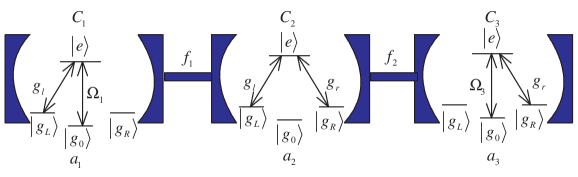
Figure 1: The structure of the experimental setup and atoms. Three identical atoms $a_{1}$, $a_{2}$ and $a_{3}$ are trapped in three separated cavities $C_{1}$, $C_{2}$ and $C_{3}$, which are linked by two fibers $f_{1}$, $f_{2}$.

For the sake of the clearness, let us first consider the physical modal that three identical atoms $a_{1}$, $a_{2}$ and $a_{3}$ are trapped in three linearly arranged optical cavities $C_{1}$, $C_{2}$ and $C_{3}$, respectively. As shown in FIG. 1, each atom possesses one excited level $|e\rangle$ and three ground states $|g_{l}\rangle$, $|g_{o}\rangle$ and $|g_{r}\rangle$. The cavities $C_{1}$ and $C_{3}$ are single-mode, the cavity $C_{2}$ are bi-mode. $C_{1}$, $C_{2}$ and $C_{3}$ are connected by the optical fibers $f_{1}$, $f_{2}$, respectively. Assuming that the transition $|e\rangle_{a_{1(3)}}\leftrightarrow|g_{o}\rangle_{a_{1(3)}}$ is resonantly driven by a external classical field with the time-dependent Rabi frequencie $\Omega_{1(3)}(t)$, while the transition $|e\rangle_{1(2)}\leftrightarrow|g_{l}\rangle_{1(2)}(|e\rangle_{2(3)}\leftrightarrow|g_{r}\rangle_{2(3)})$ is resonantly coupled to the left-circularly(right-circularly) polarized cavity mode with the coupling constant $g_{l(r)}$, respectively.

In the short-fiber limit, i.e., $(2L\bar{\nu})/(2\pi c)\ll 1$ ($L$ is the length of the fibers, $\bar{\nu}$ is the decay rate of the cavity fields into a continuum of fiber modes and $c$ is the speed of light), only one resonant mode of the fiber interacts with the cavity mode ASSMSBPRL . In the rotating frame, the Hamiltonian of the whole system can be written as $(\hbar=1)$

$$H_{tot} = H_{l}+H_{c},$$ (9)

$$H_{l} = \sum_{o=1,3}\Omega_{o}(t)|e\rangle_{a_{o}}\langle g_{0}|+H.c.,$$ (11)

$$H_{c} = g_{1l}a_{1l}|e\rangle_{a_{1}}\langle g_{l}|+g_{2l}a_{2l}|e\rangle_{a_{2}}\langle g_{l}|+g_{2r}a_{2r}|e\rangle_{a_{2}}\langle g_{r}|+g_{3r}a_{3r}|e\rangle_{a_{3}}\langle g_{r}|$$ (15)

$$+v_{1}b_{1}^{{\dagger}}(a_{1l}+a_{2l})+v_{2}b_{2}^{{\dagger}}(a_{2r}+a_{3r})+H.c.,$$

where $a_{kl}^{{\dagger}}\ (a_{kr}^{{\dagger}})$ and $a_{kl}\ (a_{kr})$ denote the creation and annihilation operators for the left-circularly (right-circularly) polarized mode of cavities $C_{k}\ (k=1,\ 2,\ 3)$, respectively; $b_{j}^{{\dagger}}$ and $b_{j}$ denote the creation and annihilation operators associated with the resonant mode of fiber $f_{j}\ (j=1,\ 2)$, respectively. For the sake of simplicity, we assume $g_{1l}=g_{2l}=g_{2r}=g_{3r}=g$ and $v_{1}=v_{2}=v$. If the initial state of the whole system is $|g_{o}g_{l}g_{r}\rangle|0\rangle_{C_{1}}|00\rangle_{C_{2}}|0\rangle_{C_{3}}|0\rangle_{f_{1}}|0\rangle_{f_{2}}$ (here $|g_{o}g_{l}g_{r}\rangle=|g_{o}g_{l}g_{r}\rangle_{a_{1}a_{2}a_{3}}$), the whole system evolves in the following subspaces

$$|\phi_{1}\rangle = |g_{o}g_{l}g_{r}\rangle|0\rangle_{C_{1}}|00\rangle_{C_{2}}|0\rangle_{C_{3}}|0\rangle_{f_{1}}|0\rangle_{f_{2}},~{}|\phi_{2}\rangle=|eg_{l}g_{r}\rangle|0\rangle_{C_{1}}|00\rangle_{C_{2}}|0\rangle_{C_{3}}|0\rangle_{f_{1}}|0\rangle_{f_{2}},$$ (16)

$$|\phi_{3}\rangle = |g_{l}g_{l}g_{r}\rangle|1\rangle_{C_{1}}|00\rangle_{C_{2}}|0\rangle_{C_{3}}|0\rangle_{f_{1}}|0\rangle_{f_{2}},~{}|\phi_{4}\rangle=|g_{l}g_{l}g_{r}\rangle|0\rangle_{C_{1}}|00\rangle_{C_{2}}|0\rangle_{C_{3}}|1\rangle_{f_{1}}|0\rangle_{f_{2}},$$ (18)

$$|\phi_{5}\rangle = |g_{l}g_{l}g_{r}\rangle|0\rangle_{C_{1}}|10\rangle_{C_{2}}|0\rangle_{C_{3}}|0\rangle_{f_{1}}|0\rangle_{f_{2}},~{}|\phi_{6}\rangle=|g_{l}eg_{r}\rangle|0\rangle_{C_{1}}|00\rangle_{C_{2}}|0\rangle_{C_{3}}|0\rangle_{f_{1}}|0\rangle_{f_{2}},$$ (20)

$$|\phi_{7}\rangle = |g_{l}g_{r}g_{r}\rangle|0\rangle_{C_{1}}|01\rangle_{C_{2}}|0\rangle_{C_{3}}|0\rangle_{f_{1}}|0\rangle_{f_{2}},~{}|\phi_{8}\rangle=|g_{l}g_{r}g_{r}\rangle|0\rangle_{C_{1}}|00\rangle_{C_{2}}|0\rangle_{C_{3}}|0\rangle_{f_{1}}|1\rangle_{f_{2}},$$ (22)

$$|\phi_{9}\rangle = |g_{l}g_{r}g_{r}\rangle|0\rangle_{C_{1}}|00\rangle_{C_{2}}|1\rangle_{C_{3}}|0\rangle_{f_{1}}|0\rangle_{f_{2}},~{}|\phi_{10}\rangle=|g_{l}g_{r}e\rangle|0\rangle_{C_{1}}|00\rangle_{C_{2}}|0\rangle_{C_{3}}|0\rangle_{f_{1}}|0\rangle_{f_{2}},$$ (24)

$$|\phi_{11}\rangle = |g_{l}g_{r}g_{o}\rangle|0\rangle_{C_{1}}|00\rangle_{C_{2}}|0\rangle_{C_{3}}|0\rangle_{f_{1}}|0\rangle_{f_{2}},$$ (26)

where $|ijk\rangle\ (i,\ j,\ k\in[e,\ g_{l},\ g_{o},\ g_{r}])$ denotes the state of the atoms in every cavity, $|n\rangle_{s}\ (s=C_{1},\ C_{3},\ f_{1},\ f_{2})$ means that the quantum field state of system contains $n$ photons. $|n_{1}n_{2}\rangle_{C_{2}}$ means that the number of left-circularly photon is $n_{1}$ and the number of right-circularly photon is $n_{2}$ in the cavity $C_{2}$.

Under the Zeno condition $g,v\gg\Omega_{1},\Omega_{3}$, the Hilbert subspace is split into nine invariant Zeno subspace

$$Z_{1} = \{|\phi_{1}\rangle,|\psi_{1}\rangle,|\phi_{11}\rangle\},~{}Z_{2}=\{|\psi_{2}\rangle\},$$ (27)

$$Z_{3} = \{|\psi_{3}\rangle\},~{}Z_{4}=\{|\psi_{4}\rangle\},~{}Z_{5}=\{|\psi_{5}\rangle\},~{}Z_{6}=\{|\psi_{6}\rangle\},$$ (29)

$$Z_{7} = \{|\psi_{7}\rangle\},~{}Z_{8}=\{|\psi_{8}\rangle\},~{}Z_{9}=\{|\psi_{9}\rangle\},$$ (31)

where the eigenstates of $H_{c}$ are

$$|\psi_{1}\rangle = N_{1}(|\phi_{2}\rangle-\frac{g}{v}|\phi_{4}\rangle+|\phi_{6}\rangle-\frac{g}{v}|\phi_{8}\rangle+|\phi_{10}\rangle),$$ (32)

$$|\psi_{2}\rangle = N_{2}(-|\phi_{2}\rangle+\varepsilon_{1}|\phi_{3}\rangle-\eta_{1}|\phi_{4}\rangle-\chi_{1}|\phi_{5}\rangle+\chi_{1}|\phi_{7}\rangle+\eta_{1}|\phi_{8}\rangle-\epsilon_{1}|\phi_{9}\rangle+|\phi_{10}\rangle),$$ (34)

$$|\psi_{3}\rangle = N_{3}(-|\phi_{2}\rangle-\varepsilon_{1}|\phi_{3}\rangle-\eta_{1}|\phi_{4}\rangle+\chi_{1}|\phi_{5}\rangle-\chi_{1}|\phi_{7}\rangle+\eta_{1}|\phi_{8}\rangle+\epsilon_{1}|\phi_{9}\rangle+|\phi_{10}\rangle),$$ (36)

$$|\psi_{4}\rangle = N_{4}(|\phi_{2}\rangle-\mu_{1}|\phi_{3}\rangle-\zeta_{1}|\phi_{4}\rangle+\delta_{1}|\phi_{5}\rangle-\theta_{1}|\phi_{6}\rangle+\delta_{1}|\phi_{7}\rangle-\zeta_{1}|\phi_{8}\rangle-\mu_{1}|\phi_{9}\rangle+|\phi_{10}\rangle),$$ (38)

$$|\psi_{5}\rangle = N_{5}(|\phi_{2}\rangle+\mu_{1}|\phi_{3}\rangle-\zeta_{1}|\phi_{4}\rangle-\delta_{1}|\phi_{5}\rangle-\theta_{1}|\phi_{6}\rangle-\delta_{1}|\phi_{7}\rangle-\zeta_{1}|\phi_{8}\rangle+\mu_{1}|\phi_{9}\rangle+|\phi_{10}\rangle),$$ (40)

$$|\psi_{6}\rangle = N_{6}(-|\phi_{2}\rangle+\varepsilon_{2}|\phi_{3}\rangle-\eta_{2}|\psi_{4}\rangle+\chi_{2}|\phi_{5}\rangle-\chi_{2}|\phi_{7}\rangle+\eta_{2}|\phi_{8}\rangle-\epsilon_{2}|\phi_{9}\rangle+|\phi_{10}\rangle),$$ (42)

$$|\psi_{7}\rangle = N_{7}(-|\phi_{2}\rangle-\varepsilon_{2}|\phi_{3}\rangle-\eta_{2}|\psi_{4}\rangle-\chi_{2}|\phi_{5}\rangle+\chi_{2}|\phi_{7}\rangle+\eta_{2}|\phi_{8}\rangle+\epsilon_{2}|\phi_{9}\rangle+|\phi_{10}\rangle),$$ (44)

$$|\psi_{8}\rangle = N_{8}(|\phi_{2}\rangle-\mu_{2}|\phi_{3}\rangle+\zeta_{2}|\phi_{4}\rangle-\delta_{2}|\phi_{5}\rangle+\theta_{2}|\phi_{6}\rangle-\delta_{2}|\phi_{7}\rangle+\zeta_{2}|\phi_{8}\rangle-\mu_{2}|\phi_{9}\rangle+|\phi_{10}\rangle),$$ (46)

$$|\psi_{9}\rangle = N_{9}(|\phi_{2}\rangle+\mu_{2}|\phi_{3}\rangle+\zeta_{2}|\phi_{4}\rangle+\delta_{2}|\phi_{5}\rangle+\theta_{2}|\phi_{6}\rangle+\delta_{2}|\phi_{7}\rangle+\zeta_{2}|\phi_{8}\rangle+\mu_{2}|\phi_{9}\rangle+|\phi_{10}\rangle),$$ (48)

with the corresponding eigenvalues

$$\lambda_{1} = 0,~{}\lambda_{2}=-\sqrt{(g^{2}+2v^{2}-A)/2},~{}\lambda_{3}=\sqrt{(g^{2}+2v^{2}-A)/2},$$ (49)

$$\lambda_{4} = -\sqrt{(3g^{2}+2v^{2}-A)/2},~{}\lambda_{5}=\sqrt{(3g^{2}+2v^{2}-A)/2},~{}\lambda_{6}=-\sqrt{(g^{2}+2v^{2}+A)/2},$$ (51)

$$\lambda_{7} = \sqrt{(g^{2}+2v^{2}+A)/2},~{}\lambda_{8}=-\sqrt{(3g^{2}+2v^{2}+A)/2},~{}\lambda_{9}=\sqrt{(3g^{2}+2v^{2}+A)/2},$$ (53)

where the parameters are

$$\epsilon_{1} = \frac{\sqrt{g^{2}+2v^{2}-A}}{\sqrt{2}g},~{}\eta_{1}=\frac{-g^{2}+2v^{2}-A}{2gv},~{}\chi_{1}=\frac{\sqrt{g^{2}+2v^{2}-A}(g^{2}+A)}{2\sqrt{2}gv^{2}},$$ (54)

$$\mu_{1} = \frac{\sqrt{3g^{2}+2v^{2}-A}}{\sqrt{2}g},~{}\zeta_{1}=\frac{-g^{2}-2v^{2}+A}{2gv},~{}\delta_{1}=\frac{\sqrt{3g^{2}+2v^{2}-A}(-g^{2}+A)}{2\sqrt{2}gv^{2}},~{}\theta_{1}=\frac{-g^{2}+A}{v^{2}},$$ (56)

$$\epsilon_{2} = \frac{\sqrt{g^{2}+2v^{2}+A}}{\sqrt{2}g},~{}\eta_{2}=\frac{-g^{2}+2v^{2}+A}{2gv},~{}\chi_{2}=\frac{\sqrt{g^{2}+2v^{2}+A}(-g^{2}+A)}{2\sqrt{2}gv^{2}},$$ (58)

$$\mu_{2} = \frac{\sqrt{3g^{2}+2v^{2}+A}}{\sqrt{2}g},~{}\zeta_{2}=\frac{g^{2}+2v^{2}+A}{2gv},~{}\delta_{2}=\frac{\sqrt{3g^{2}+2v^{2}+A}(g^{2}+A)}{2\sqrt{2}gv^{2}},~{}\theta_{2}=\frac{g^{2}+A}{v^{2}},$$ (60)

in addition, $A=\sqrt{g^{4}+4v^{4}}$ and $N_{w}$ is the normalization factor of the eigenstate $|\psi_{w}\rangle\ (w=1,2,\cdots,9)$.

The projector in the $k$th Zeno subspace $Z_{k}$ is

$$P_{k}^{\beta}=|\beta\rangle\langle\beta|,\ (|\beta\rangle\in Z_{k}).$$ (61)

The Hamiltonian in Eq. (8) can be approximately given by

$$H_{tot} \simeq \sum_{k,\beta,\gamma}{\lambda_{k}P_{k}^{\beta}+P_{k}^{\beta}H_{l}P_{k}^{\gamma}}$$ (62)

$$= \sum_{k=2}^{9}{\lambda_{k}|\psi_{k}\rangle\langle\psi_{k}|+N_{1}(\Omega_{1}|\phi_{1}\rangle\langle\psi_{1}|+\Omega_{3}|\phi_{11}\rangle\langle\psi_{1}|+H.c.)}.$$ (64)

If the initial state is $|g_{o}g_{l}g_{r}\rangle|0\rangle_{C_{1}}|00\rangle_{C_{2}}|0\rangle_{C_{3}}|0\rangle_{f_{1}}|0\rangle_{f_{2}}$, it reduces to

$$H_{eff}=N_{1}(\Omega_{1}|\phi_{1}\rangle\langle\psi_{1}|+\Omega_{3}|\phi_{11}\rangle\langle\psi_{1}|+H.c.),$$ (65)

which can be treated as a simple three-level system with an excited state $|\psi_{1}\rangle$ and two ground states $|\phi_{1}\rangle$ and $|\phi_{11}\rangle$. Then we obtain the eigenvectors and eigenvalues of the effective Hamiltonian $H_{eff}$ as

$$|\eta_{o}(t)\rangle=\left(\begin{array}[]{c}\cos\theta(t)\\ 0\\ -\sin\theta(t)\end{array}\right),~{}|\eta_{\pm}(t)\rangle=\frac{1}{\sqrt{2}}\left(\begin{array}[]{c}\sin\theta(t)\\ \pm 1\\ \cos\theta(t)\end{array}\right),$$ (72)

with the corresponding eigenvalues $\eta_{0}=0$ and $\eta_{\pm}=\pm N_{1}\Omega$, and $\tan\theta=\frac{\Omega_{1}}{\Omega_{3}}$ and $\Omega=\sqrt{\Omega_{1}^{2}+\Omega_{3}^{2}}$.

IV The generation of the three-atom GHZ state via transitionless quantum driving and adiabatic passage

IV.1 Adiabatic passage method

For the sake of the clearness, we first briefly present how to generate the three-atom GHZ state via adiabatic passage. When the adiabatic condition $|\langle n_{0}|\partial_{t}n_{\pm}\rangle|\ll|\lambda_{\pm}^{\prime}|$ is fulfilled well and the initial state is $|\psi(0)\rangle=|\phi_{1}\rangle$, the state evolution will always follow $|n_{0}(t)\rangle$ closely. To generate the three-atom GHZ states via the adiabatic passage and meet the boundary conditions of the fractional stimulated Raman adiabatic passage (STIRAP),

$$\lim_{t\rightarrow-\infty}{\frac{\Omega_{1}(t)}{\Omega_{3}(t)}}=0,~{}\lim_{t\rightarrow+\infty}{\frac{\Omega_{3}(t)}{\Omega_{1}(t)}}=\tan{\alpha},$$ (73)

we need properly to tailor the Rabi frequencies $\Omega_{1}(t)$ and $\Omega_{3}(t)$ in the original Hamiltonian $H_{tot}$

$$\Omega_{1}(t) = \sin{\alpha}\Omega_{0}\exp{[\frac{-(t-t_{0}-t_{f}/2)^{2}}{t_{c}^{2}}]},$$ (74)

$$\Omega_{3}(t) = \Omega_{0}\exp{[\frac{-(t+t_{0}-t_{f}/2)^{2}}{t_{c}^{2}}]}+\cos{\alpha}\Omega_{0}\exp{[\frac{-(t-t_{0}-t_{f}/2)^{2}}{t_{c}^{2}}]},$$ (76)

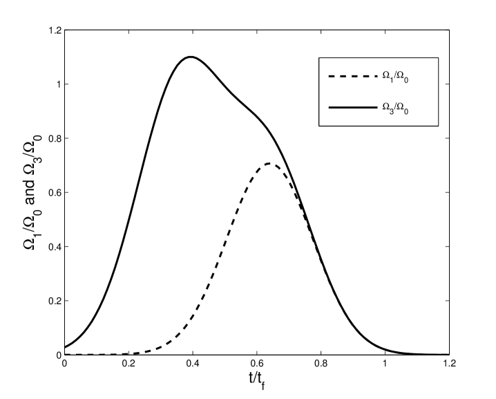
Figure 2: The laser pulses $\Omega_{1}/\Omega_{0}$ and $\Omega_{3}/\Omega_{0}$ versus $t/t_{f}$.

where $\Omega_{0}$ is the pulse amplitude and $t_{f}$ is the operation time. $t_{c}$ and $t_{0}$ are some related parameters to be chosen for the best performance of the adiabatic passage process. In order to achieve better performance and meet the boundary conditions, we suitably chose the parameters that $\tan{\alpha}=1$, $t_{0}=0.14t_{f}$ and $t_{c}=0.19t_{f}$. As shown in Fig. 2, the time-dependent $\Omega_{1}(t)/\Omega_{0}$ and $\Omega_{3}(t)/\Omega_{0}$ versus $t/t_{f}$ are plotted with the fixed values $t_{0}$ and $t_{c}$. With the above parameters, we obtain our wanted three-atom GHZ state $|\psi(t_{f})\rangle=(|\phi_{1}\rangle-|\phi_{11}\rangle)/\sqrt{2}$ via the adiabatic passage. But this evolution process needs a relatively long time to satisfy the adiabatic condition. We will detail the reasons in the section of numerical simulations and analyses.

IV.2 Transitionless quantum driving method

To reduce the evolution time and obtain the same state as the adiabatic passage, we use the approach of TQD to construct STAP. As introduced in the above, STAP speeds up a slow adiabatic passage via a non-adiabatic passage route to achieve a same outcome, and the TQD method is a important route to construct shortcuts. According to the ideas proposed by Berry Berry2009 , the instantaneous states in Eq. (16) do not meet the Schrödinger equation, i.e., $i\partial_{t}|n_{k}\rangle\neq H_{eff}|n_{k}\rangle(k=0,\pm)$, so the situation that the system starts from the state $|\psi_{n}(0)\rangle$ and ends up in the state $|\psi_{m\neq n}(t)\rangle$ occurs in a finite probability even under the adiabatic condition. To drive the instantaneous states $|n_{k}\rangle(k=0,\pm)$ exactly, we look for a Hamiltonian $H(t)$ related to the original Hamiltonian $H_{eff}$ according to Berry’s transitionless tracking algorithm Berry2009 . From section II, we know the simplest Hamiltonian $H(t)$ possessed the form,

$$H(t)=i\sum_{0,\pm}|\partial_{t}n_{k}(t)\rangle\langle n_{k}(t)|.$$ (77)

Substituting Eq. (16) in Eq. (19), we obtain

$$H(t)=i\dot{\theta}|\phi_{1}\rangle\langle\phi_{11}|+H.c.,$$ (78)

where $\dot{\theta}=[\dot{\Omega}_{1}(t)\Omega_{3}(t)-\Omega_{1}(t)\dot{\Omega}_{3}(t)]/\Omega^{2}$. This is our wanted CCD Hamiltonian to construct STAP, and we will detail how to construct this Hamiltonian in experiment later.

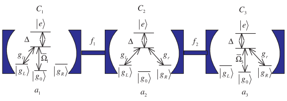
Figure 3: The structure of the experimental setup and atoms for the APF Hamiltonian.

For the present system, the CDD Hamiltonian $H(t)$ is given in Eq. (18), but it is irrealizable under current experimental condition. Inspired by Refs. [17, 19], we find an alternative physically feasible (APF) Hamiltonian whose effect is equivalent to $H_{1}(t)$. The design is shown in Fig. 3, the atomic transitions is not resonantly coupled to the classical lasers and cavity modes with the detuning $\Delta$. The Hamiltonian of the system reads $H_{tot}^{\prime}=H_{c}+H_{l}+H_{d}$, where $H_{d}=\sum_{k=1}^{3}{\Delta|e\rangle_{k}\langle e|}$. Then, similar to the approximation by QZD in section III, we also obtain an effective Hamiltonian for the non-resonant system

$$H_{eff}^{\prime}=N_{1}(\overline{\Omega}_{1}|\phi_{1}\rangle\langle\psi_{1}|+\overline{\Omega}_{3}|\phi_{11}\rangle\langle\psi_{1}|+H.c.)+3\Delta N_{1}^{2}|\psi_{1}\rangle\langle\psi_{1}|.$$ (79)

When the large detuning condition $3\Delta N_{1}\geq\overline{\Omega}_{1},\ \overline{\Omega}_{3}$ is satisfied, we can adiabatically eliminate the state $|\psi_{1}\rangle$ and obtain the final effective Hamiltonian

$$H_{fe}=-\frac{\overline{\Omega}_{1}^{2}}{3\Delta}|\phi_{1}\rangle\langle\phi_{1}|-\frac{\overline{\Omega}_{3}^{2}}{3\Delta}|\phi_{11}\rangle\langle\phi_{11}|-\frac{\overline{\Omega}_{1}\overline{\Omega}_{3}}{3\Delta}(|\phi_{1}\rangle\langle\phi_{11}|+|\phi_{11}\rangle\langle\phi_{1}|).$$ (80)

For simplicity, we set $\overline{\Omega}_{1}=\overline{\Omega}_{3}=\overline{\Omega}(t)$. The front two terms caused by Stark shift can be removed and the Hamiltonian becomes

$$\overline{H}(t)=\Omega_{x}|\phi_{1}\rangle\langle\phi_{11}|+H.c.,$$ (81)

where $\Omega_{x}=-\frac{\overline{\Omega}^{2}}{3\Delta}$. The equation has a similar form with Eq. (20), but the effective couplings between $i\dot{\theta}$ and $\Omega_{x}$ exist $3\pi/2$-dephased. To guarantee their consistency, we put a change that $\Omega_{3}\rightarrow-i\Omega_{3}$. Then, the eigenstates of $H_{eff}$ become

$$|\eta_{o}^{\prime}(t)\rangle=\left(\begin{array}[]{c}\cos\theta(t)\\ 0\\ i\sin\theta(t)\end{array}\right),~{}|\eta_{\pm}^{\prime}(t)\rangle=\frac{1}{\sqrt{2}}\left(\begin{array}[]{c}\sin\theta(t)\\ \pm 1\\ -i\cos\theta(t)\end{array}\right),$$ (88)

and the CDD Hamiltonian $H(t)$ becomes

$$H(t)=-\dot{\theta}|\phi_{1}\rangle\langle\phi_{11}|-\dot{\theta}|\phi_{11}\rangle\langle\phi_{1}|.$$ (89)

Compared Eq. (23) with Eq. (25), we can easily get the CDD Hamiltonian when the condition $\Omega_{x}=-\dot{\theta}$ is satisfied.

$$\overline{\Omega}_{1}(t)=\overline{\Omega}_{3}(t)=\overline{\Omega}(t)=\sqrt{3\Delta\dot{\theta}}.$$ (90)

IV.3 Numerical simulations and analyses

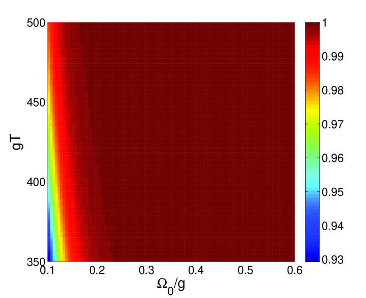
Figure 4: The fidelity versus the laser pulses amplitude $\Omega_{0}$ and the operation time $t/t_{f}$.

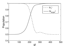
FIG. 5: (a) The population $P_{target}$ of the target state $|\psi_{target}\rangle$ and the population $P_{0}$ of the initial state $|\psi(0)\rangle$ governed by the original Hamiltonian $H_{tot}$ via the adiabatic passage. (b) The population $P_{1}(t)$ of the states $|\phi_{1}\rangle$ and the population $P_{11}(t)$ of the states $|\phi_{11}\rangle$ governed by the original Hamiltonian $H_{tot}$ via adiabatic passage. The parameters are collectively with the fixed values $\Omega_{0}=0.2g$, $g=v$, $t_{0}=0.14t_{f}$, $t_{c}=0.19t_{f}$ and $t_{f}=400/g$.

Next we will show that it takes less time to get the target state on the situation governed by the APF Hamiltonian $H_{tot}^{\prime}$ via TQD than by the original Hamiltonian $H_{tot}$ via adiabatic passage. The time-dependent population for any state $|\psi\rangle$ is defined as $P=|\langle\psi|\rho(t)|\psi\rangle|$, where $\rho(t)$ is the corresponding time-dependent density operator. We present the fidelity versus the laser pulses amplitude $\Omega_{o}$ and the operation time $t/t_{f}$ via adiabatic passage in Fig. 4. As shown in Fig. 4, we can know that the bigger the laser pulse amplitude is, the less time that the system evolution to the target state needs. However, we need to satisfy the Zeno conditions $g,v\gg\Omega_{1},\Omega_{3}$, so we set $\Omega_{0}=0.2g$. In Fig. 5, we display the time-dependent populations of the states $|\phi_{1}\rangle$, $|\psi_{target}\rangle$, and $|\phi_{11}\rangle$ via adiabatic passage. As depicted in Fig. 4 and Figs. 5, the operation time needs $t_{f}\geq 400/g$ to achieve an ideal result at least. It is awkward in some case.

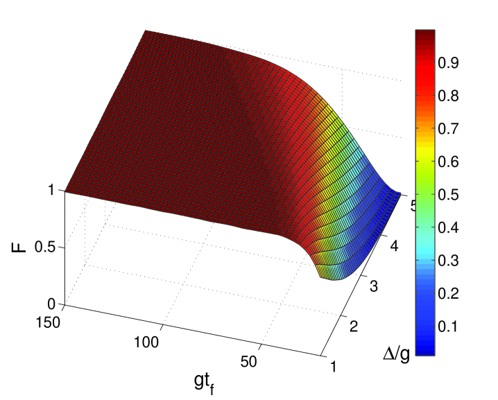
Figure 6: The fidelity $F$ of the target state $|\psi(t_{f})\rangle$ governed by $H_{tot}^{\prime}$ versus the interaction time $gt_{f}$ and the detuning $\Delta/g$.

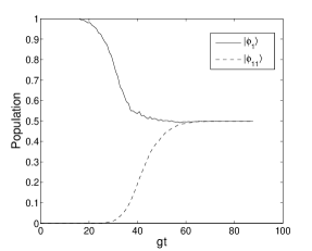
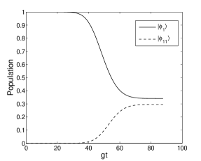
FIG. 7: The population $P_{1}(t)$ of the state $|\phi_{1}\rangle$ and the population $P_{11}(t)$ of the state $|\phi_{11}\rangle$ governed by (a) the APF Hamiltonian $H_{tot}^{\prime}$ with $\Delta=2.3g$. (b) The original Hamiltonian $H_{tot}$ collectively with the fixed values $\Omega_{0}=0.2g$, $g=v$, $t_{0}=0.14t_{f}$, $t_{c}=0.19t_{f}$, and $t_{f}=72/g$.

Next we will detail the evolution governed by the APF Hamiltonian $H_{tot}^{\prime}$ via TQD. According to eq. (24) we finally get a GHZ state $|\psi(t_{f})=\frac{1}{\sqrt{2}}(|\phi_{1}\rangle+i|\phi_{11}\rangle)$. In Fig. 6, we present the relationship between the fidelity of the three-atom GHZ state (governed by the APF Hamiltonian) and two parameters $\Delta$ and $t_{f}$ when $\Omega_{0}=0.2g$ to satisfy the Zeno condition, where the fidelity of the three-atom GHZ state is defined as $F=|\langle GHZ|\rho(t_{f})|GHZ\rangle|$ ($\rho(t_{f})$ is the desity operator of the whole system when $t=t_{f}$). We find that a wide range for parameters $\Delta$ and $t_{f}$ can obtain a high fidelity of the three-atom GHZ state, and the fidelity increases with the increasing of $\Delta$ and the decreasing of $t_{f}$. In order to satisfy the large detuning condition, we set $\Delta=2.3g$. The Fig. 6 reveals that the operation time needs $t_{f}\geq 72/g$ via TQD at least. In Figs. 7 we plot the operation time for the creation of the GHZ state governed by $H_{tot}^{\prime}$ and by $H_{tot}$ with the parameters that $t_{f}=72/g$, $\Omega_{0}=0.2g$, $\Delta=2.3g$ and $g=v$. Numerical results show that the APF Hamiltonian $H_{tot}^{\prime}$ can govern the evolution to a perfect GHZ state $|\psi(t_{f})\rangle$ from $|\psi_{1}\rangle$ in a relatively short interaction time while the original Hamiltonian $H_{tot}$ can not.

In above analysis, we do not consider the influence of decoherence caused by various factors, such as spontaneous emissions, cavity decays and fiber photon leakages. In fact, the decoherence is unavoidable during the evolution of the whole system in experiment. The master equation of the whole system is written as

$$\dot{\rho} = -i[H_{tot},\rho]$$ (99)

$$+\sum_{k=1}^{3}\frac{\gamma_{k}}{2}(2\sigma_{k}^{-}\rho\sigma_{k}^{+}-\sigma_{k}^{+}\sigma_{k}^{-}\rho-\rho\sigma_{k}^{+}\sigma_{k}^{-})$$

$$+\sum_{k=1}^{2}\frac{\kappa_{c_{k}}}{2}(2a_{l,k}\rho a_{l,k}^{+}-a_{l,k}^{+}a_{l,k}\rho-\rho a_{l,k}^{+}a_{l,k})$$

$$+\sum_{k=2}^{3}\frac{\kappa_{c_{k}}}{2}(2a_{r,k}\rho a_{r,k}^{+}-a_{r,k}^{+}a_{r,k}\rho-\rho a_{r,k}^{+}a_{r,k})$$

$$+\sum_{k=1}^{2}\frac{\kappa_{f_{k}}}{2}(2b_{k}\rho b_{k}^{+}-b_{k}^{+}b_{k}\rho-\rho b_{k}^{+}b_{k}),$$

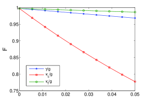
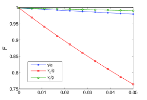
FIG. 8: The fidelity of the target state $|\psi(t_{f})\rangle$ governed by (a) the APF Hamiltonian $H_{tot}^{\prime}$ with $\Delta=2.3g$, $t_{f}=72/g$ and $\Omega_{0}=0.2g$. (b) the original Hamiltonian $H_{tot}$ with $t_{f}=153/g$, and $\Omega_{0}=0.5g$ collectively with the fixed values $t_{0}=0.14t_{f}$, and $t_{c}=0.19t_{f}$ versus the dimensionless parameters $\gamma/g$, $\kappa_{c}/g$, and $\kappa_{f}/g$, respectively.

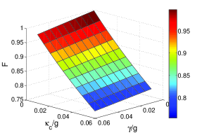
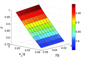
FIG. 9: The fidelity of the target state $|\psi(t_{f})\rangle$ governed by (a) the APF Hamiltonian $H_{tot}^{\prime}$ with $\Delta=2.3g$, $t_{f}=72/g$, and $\Omega_{0}=0.2g$. (b) the original Hamiltonian $H_{tot}$ with $t_{f}=153/g$, and $\Omega_{0}=0.5g$ collectively with the fixed values $t_{0}=0.14t_{f}$, and $t_{c}=0.19t_{f}$ versus the dimensionless parameters $\gamma/g$ and $\kappa_{c}/g$.

where $\gamma_{k}$ is the atomic spontaneous emission rate for the $k$th atom and $\kappa_{c(f)}$ is the decay rate of the $k$th cavity ($k$th fiber), $\sigma_{k}^{-}$ denotes the atomic transition from the ground states $|m\rangle\ (m=g_{0},\ g_{l},\ g_{r})$ to the excited state $|e\rangle$. For the sake of simplicity, we assume that $\gamma_{1}=\gamma_{2}=\gamma_{3}=\gamma$, $\kappa_{c_{1}}=\kappa_{c_{2}}=\kappa_{c_{3}}=\kappa_{c}$ and $\kappa_{f_{1}}=\kappa_{f_{2}}=\kappa_{f}$. As shown in Fig. 8, we plot the fidelity governed by the APF Hamiltonian $H_{tot}^{\prime}$ and by the original Hamiltonian $H_{tot}$ and the dimensionless parameters $\gamma/g$, $\kappa_{c}/g$ and $\kappa_{f}/g$, respectively. We can draw a conclusion that the fidelities are almost unaffected by the fiber decay both via TQD and via adiabatic passage. We focus on the main decoherence factors included the cavity decay and the atomic spontaneous emission. As shown in Figs. 9, we plot the fidelity versus the cavity decay and the atomic spontaneous emission. We can know the most important decoherence factor is the cavity decay. This result can be understood from Ref. [18] that if the Zeno condition can not be satisfied very well, the populations of the intermediate states including the cavity excited states can not be suppressed ideally.

From the above anslysis, we can obviously know that the evolution time from the initial state to the target state via TQD is $t_{f}=72/g$ when $\Omega_{0}=0.2g$, $\Delta=2.3g$, $t_{0}=0.14t_{f}$, $t_{c}=0.19t_{f}$ and $g=v$, while the evolution time for the adiabatic passage is $t_{f}=400/g$ when $\Omega_{0}=0.2g$, $t_{0}=0.14t_{f}$, $t_{c}=0.19t_{f}$ and $g=v$. So, the benefit of the TQD method is shown obviously that the speed via TQD method is faster than that via adiabatic passage. It is more worthy to note that the fidelity of the target state via TQD is almost equal to that via adiabatic passage. So our scheme has a huge advantage compared with the proposals via adiabatic passage. That means the present scheme via STAP method is not only fast but also robust.

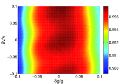
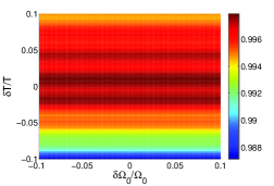
FIG. 10: The fidelity of the target state $|\psi_{target}\rangle$ versus the deviations of (a) $g$ and $v$, (b) $T$ and $\Omega_{0}$.

As we all know, it is necessary for a good scheme to tolerate the deviations of the experimental parameters, because it is impossible to avoid the operational imperfection in experiment. Define that $\delta x=x^{\prime}-x$ is the deviation of the ideal value $x$, $x^{\prime}$ is the actual value. In Fig. 10, we plot the fidelity of the target state $|\psi_{target}\rangle$ versus the deviations of the experimental parameters $g$, $v$, $\Omega_{0}$, and $T$ ($T=t_{f}$ denotes the operation time). Numerical results demonstrate that our scheme is robust against the fluctuation of the experimental parameters.

V the generation of the $N$-atom GHZ state via transitionless quantum driving

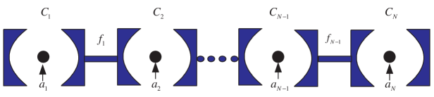
Figure 11: The set-up diagram for the generation of $N$-atom GHZ states. The $N$-atoms are respectively trapped in $N$-cavities which are linked by $N-1$ fibers.

Next we briefly present the generalization of the scheme in Section IV to generate $N$-atom GHZ state by the same principle. We consider the physical configuration shown in Fig. 11, where $N$ atoms $a_{1},\ a_{2},\ \cdots,\ a_{N}$ are trapped in $N$ cavities $C_{1},\ C_{2},\ \cdots,\ C_{N}$ connected by $N-1$ fibers $f_{1},\ f_{2},\ \cdots,\ f_{N-1}$, respectively. The level configurations of the atoms between two ends are the same as that of the atom $a_{2}$ in the three-atom case, and the level configurations of $a_{1}$ and $a_{N}$ are the same as those of $a_{1}$ and $a_{3}$ in the three-atom case, respectively. The Hamiltonian of the present system can be written as in the rotation framework

$$H_{total} = H_{l}^{\prime}+H_{c}^{\prime},$$ (100)

$$H_{l}^{\prime} = \Omega_{1}^{\prime}|e\rangle_{a_{1}}\langle g_{0}|+\Omega_{N}^{\prime}|e\rangle_{a_{N}}\langle g_{0}|+H.c.,$$ (102)

$$H_{c}^{\prime} = \sum_{i=1}^{N-1}{g_{i,l}a_{i,l}|e\rangle_{a_{i}}\langle g_{l}|}+\sum_{j=2}^{N}{g_{j,r}a_{j,r}|e\rangle_{a_{j}}\langle g_{r}|}$$ (104)

$$+ \sum_{k=2}^{N-1}{[v_{k-1}b_{k-1}^{{\dagger}}(a_{k-1,l}+a_{k,l})+v_{k}b_{k}^{{\dagger}}(a_{k,r}+a_{k+1,r})]}+H.c..$$ (106)

Let us consider the situation where $N$ is an odd number, i.e., $N=2l+1,\ (l=1,\ 2,\ 3,\cdots)$. Suppose that the initial state of the atoms is $|g_{0}g_{l}g_{r}g_{l}g_{r}\ \cdots\ g_{r}\rangle$ while all the cavities and fibers are vacuum, then the system can be expended in the following subspace

$$|\phi_{1}^{\prime}\rangle=|g_{0}g_{l}g_{r}\ \cdots\ g_{r}\rangle|0\rangle_{all},~{}|\phi_{2}^{\prime}\rangle=|eg_{l}g_{r}\ \cdots\ g_{r}\rangle|0\rangle_{all},$$ (107)

(108)

$$|\phi_{3}^{\prime}\rangle=|g_{l}g_{l}g_{r}\ \cdots\ g_{r}\rangle|1\rangle_{c_{1}},~{}|\phi_{4}^{\prime}\rangle=|g_{l}g_{l}g_{r}\ \cdots\ g_{r}\rangle|1\rangle_{f_{1}},$$ (109)

(110)

$$|\phi_{5}^{\prime}\rangle=|g_{l}g_{l}g_{r}\ \cdots\ g_{r}\rangle|10\rangle_{c_{2}},~{}|\phi_{6}^{\prime}\rangle=|g_{l}eg_{r}\ \cdots\ g_{r}\rangle|0\rangle_{all},$$ (111)

(112)

$$|\phi_{7}^{\prime}\rangle=|g_{l}g_{r}g_{r}\ \cdots\ g_{r}\rangle|01\rangle_{c_{2}},~{}|\phi_{8}^{\prime}\rangle=|g_{l}g_{r}g_{r}\ \cdots\ g_{r}\rangle|1\rangle_{f_{2}},$$ (113)

(114)

$$|\phi_{9}^{\prime}\rangle=|g_{l}g_{r}g_{r}\ \cdots\ g_{r}\rangle|01\rangle_{c_{3}},~{}|\phi_{10}^{\prime}\rangle=|g_{l}g_{r}e\ \cdots\ g_{r}\rangle|0\rangle_{all},\cdots$$ (115)

(116)

$$|\phi_{4N-1}^{\prime}\rangle=|g_{l}g_{r}\ \cdots\ g_{r}g_{0}\rangle|0\rangle_{all},$$ (117)

where $|0\rangle_{all}$ means that there is none photon in all boson modes, $|n_{1}n_{2}\rangle_{s_{i}}\ (s=C,\ f.\ i=1,\ 2,\cdots,N)$ means that there are $n_{1}$ left-circularly photon and $n_{2}$ right-circularly photon in the corresponding cavity $C_{i}$ or fiber $f_{i}$.

Similar to the above procedure from Eq. (10) to Eq. (16), we get an effective Hamiltonian

$$H_{eff(N)}=N_{1}^{\prime}(\Omega_{1}^{\prime}|\phi_{1}^{\prime}\rangle\langle\psi_{1}^{\prime}|+\Omega_{N}^{\prime}|\phi_{4N-1}^{\prime}\rangle\langle\psi_{1}^{\prime}|+H.c.),$$ (118)

where

$$|\psi_{1}^{\prime}\rangle=N_{1}^{\prime}(\sum_{i=1}^{N}|\phi_{4i-2}^{\prime}\rangle-\sum_{i=1}^{N-1}\frac{g}{v}|\phi_{4i}^{\prime}\rangle).$$ (119)

In addition, the eigenstates and eigenvalues of the Hamiltonian in Eq. (30) can be written as

$$|\chi_{o}(t)\rangle=\left(\begin{array}[]{c}\cos\theta^{\prime}(t)\\ 0\\ -\sin\theta^{\prime}(t)\end{array}\right),~{}|\chi_{\pm}(t)\rangle=\frac{1}{\sqrt{2}}\left(\begin{array}[]{c}\sin\theta^{\prime}(t)\\ \pm 1\\ \cos\theta^{\prime}(t)\end{array}\right),$$ (126)

with the corresponding eigenvalues $\chi_{0}^{\prime}=0$ and $\chi_{\pm}^{\prime}=\pm N_{1}^{\prime}\Omega^{\prime}$, where $\tan\theta^{\prime}=\frac{\Omega_{1}^{\prime}}{\Omega_{N}^{\prime}}$ and $\Omega^{\prime}=\sqrt{\Omega_{1}^{\prime 2}+\Omega_{N}^{\prime 2}}$. Substituting Eq. (32) in Eq. (19), we obtain

$$H^{\prime}(t)=i\dot{\theta}^{\prime}|\phi_{1}^{\prime}\rangle\langle\phi_{4N-1}^{\prime}|+H.c.,$$ (127)

where $\dot{\theta}^{\prime}=[\dot{\Omega}_{1}^{\prime}(t)\Omega_{N}^{\prime}(t)-\Omega_{1}^{\prime}(t)\dot{\Omega}_{N}^{\prime}(t)]/\Omega^{\prime 2}$.

Inspired by the above idea in section IV, we make the system into a non-resonant system to construct the CDD Hamiltonian in Eq. (33). Therefore, the Hamiltonian of the present system reads $H_{total}^{\prime}=H_{l}^{\prime}+H_{c}^{\prime}+H_{d}^{\prime}$, where $H_{d}^{\prime}=\sum_{i=1}^{N}\Delta|e\rangle\langle e|$. Similar to the above procedure from Eq. (80) to Eq. (81) in Section IV, we obtain the final effective Hamiltonian

$$H_{fe(N)}^{\prime}=-\frac{\overline{\Omega}_{1}^{\prime 2}}{3\Delta}|\phi_{1}^{\prime}\rangle\langle\phi_{1}^{\prime}|-\frac{\overline{\Omega}_{N}^{\prime 2}}{3\Delta}|\phi_{4N-1}^{\prime}\rangle\langle\phi_{4N-1}^{\prime}|-\frac{\overline{\Omega}_{1}^{\prime}\overline{\Omega}_{N}^{\prime}}{3\Delta}(|\phi_{1}^{\prime}\rangle\langle\phi_{4N-1}^{\prime}|+|\phi_{4N-1}^{\prime}|\rangle\langle\phi_{1}^{\prime}|).$$ (128)

For simplicity, we set $\overline{\Omega}_{1}^{\prime}=\overline{\Omega}_{N}^{\prime}=\overline{\Omega}^{\prime}$, the front two terms caused by Stark shift can be omitted and the Hamiltonian becomes

$$\overline{H}_{N}=\Omega_{x}^{\prime}(t)|\phi_{1}^{\prime}\rangle\langle\phi_{4N-1}^{\prime}|+H.c.,$$ (129)

where $\Omega_{x}^{\prime}(t)=-\frac{\overline{\Omega}^{\prime 2}}{3\Delta}$. To guarantee their consistency, we put a change that $\Omega_{N}\rightarrow-i\Omega_{N}$. Then the eigenstates of $H_{eff(N)}$ become

$$|\chi_{o}^{\prime}(t)\rangle=\left(\begin{array}[]{c}\cos\theta^{\prime}(t)\\ 0\\ i\sin\theta^{\prime}(t)\end{array}\right),~{}|\chi_{\pm}^{\prime}(t)\rangle=\frac{1}{\sqrt{2}}\left(\begin{array}[]{c}\sin\theta^{\prime}(t)\\ \pm 1\\ -i\cos\theta^{\prime}(t)\end{array}\right),$$ (136)

and the CDD Hamiltonian $H(t)$ becomes

$$H^{\prime}(t)=-\dot{\theta}^{\prime}|\phi_{1}^{\prime}\rangle\langle\phi_{4N-1}^{\prime}|-\dot{\theta}^{\prime}|\phi_{4N-1}^{\prime}\rangle\langle\phi_{1}^{\prime}|.$$ (137)

Compared Eq. (35) with Eq. (37), we can easily get the CDD Hamiltonian when the condition $\Omega_{x}^{\prime}=-\dot{\theta}^{\prime}$ is satisfied.

$$\overline{\Omega}_{1}^{\prime}(t)=\overline{\Omega}_{N}^{\prime}(t)=\overline{\Omega}^{\prime}(t)=\sqrt{3\Delta\dot{\theta}^{\prime}}.$$ (138)

VI experimental feasibility and conclusions

Now experimental feasibility needs to be discussed. The configuration of ${}^{87}Rb$ can be suitable for our proposals. Under current experimental condition a set of CQED parameters $g=2\pi\times 750MHz$, $\gamma=2\pi\times 2.62MHz$, and $\kappa_{c}=2\pi\times 3.5MHz$ are available with the wavelength in the region $630-850$nm SMSTJKKJVKWGEWHJKPRA . By using fiber-taper coupling to high-Q silica microspheres the efficiency of fiber-cavity coupling is higher than $99.9\%$ SMSTJKOJPKJVPRL . The optical fiber decay at a 852nm wavelength is about 2.2dB/km KJGVFPDTGSB , which means the fiber decay rate is about $\kappa_{f}=1.52\times 10^{5}Hz$. With the above parameters, we obtain a relatively high fidelity about $97.15\%$.

In conclusion, we have proposed an efficient scheme to fast deterministically generate $N$-atom GHZ state in separate coupled cavities via transitionless quantum driving (TQD) only by one-step manipulation. We apply a promising method to construct STAP by joint utilization of the Zeno dynamics and the approach of TQD in the cavities QED system. The method features are that we do not need to control the time exactly and the evolution process is fast. Because the atoms are trapped in separate coupled cavity, the single qubit manipulation can be realized easily. When considering dissipation, we can see that the method is robust against the decoherences caused by the atomic spontaneous emission and fiber decay. The results show that the scheme has a high fidelity and may be possible to implement with the current experimental technology. So, the scheme is fast, robust and effective. We hope the scheme can be used to generate multi-atom GHZ state in the future.

References

- (1) S. B. Zheng and G. C. Guo, “Efficient scheme for two-atom entanglement and quantum information processing in cavity QED,” Phys. Rev. Lett. 85, 2392-2395 (2000).
- (2) J. S. Bell, “On the Einstein-Podolsky-Rosen paradox,” Physics 1, 195-200 (1965).
- (3) M. A. Nielsen and I. L. Chuang, “Quantum computation and quantum information,” Cambridge University Press, Cambridge, (2000).
- (4) A. K. Ekert, “Quantum cryptography based on Bell’s theorem,” Phys. Rev. Lett. 67, 661-663 (1991).
- (5) Y. Xia, J. Song, P. M. Lu, and H. S. Song, “Teleportation of an -photon Greenberger-Horne-Zeilinger (GHZ) polarization entangled state using linear optical elements,” J. Opt. Soc. Am. B 27, A1-A6 (2010).
- (6) C. H. Bennett, G. Brassard, C. Crepeau, R. Jozsa, A. Peres, and W. Wootters, “Teleporting an unknown quantum state via dual classical and Einstein-Podolsky-Rosen channels,” Phys. Rev. Lett. 70, 1895-1899 (1993).
- (7) M. Hillery, V. Buzek, and A. Berthiaume, “Quantum secret sharing,” Phys. Rev. A 59, 1829-1834 (1999).
- (8) D. M. Greenberger, M. A. Horne, and A. Zeilinger, in Bell’s Theorem, Quantum Theory, and Conception of the Universe, M. Kafators, (Kluwer, 1989),pp. 69-72; D. M. Greenberger, M. Horne, A. Shimony, and A. Zeilinger, “Bell’s theorem without inequalities,” Am. J. Phys. 58, 1131-1142 (1990).
- (9) S. B. Zheng, “Generation of Greenberger-Horne-Zeilinger states for multiple atoms trapped in separated cavities,” Eur. Phys. J. D 54, 719-722 (2009).
- (10) S. B. Zheng, “One-step synthesis multiatom Greenberger-Horne-Zeilinger states,” Phys. Rev. Lett. 87, 230404 (2001).
- (11) D. Leibfried, E. Knill, S. Seidelin, J. Britton, R. B. Blakestad, J. Chiaverini, D. B. Hume, W. M. Itano, J. D. Jost, C. Langer, R. Ozeri, R. Reichle, and D. J. Wineland, “Creation of a six-atom ‘Schrödinger cat’ state,” Nature 438, 639-642 (2005).
- (12) Z. Zhao, Y. A. Chen, A. N. Zhang, T. Yang, H. J. Briegel, and J. W. Pan, “Experimental demonstration of five-photon entanglement and open-destination teleportation,” Nature 430, 54-58 (2004).
- (13) X. L. Su, A. H. Tan, X. J. Jia, J. Zhang, C. D. Xie, and K. C. Peng, “Experimental preparation of quadripartite cluster and Greenberger-Horne-Zeilinger states for continuous variables,” Phys. Rev. Lett. 98, 070502 (2007).
- (14) J. M. Raimond, M. Brune, and S. Haroche, “Manipulating quantum entanglement with atoms and photons in a cavity,” Rev. Mod. Phys. 73, 565 (2001).
- (15) Z. C. Shi, Y. Xia, J. Song, and H. S. Song, “One-step implementation of the Fredkin gate via Zeno dynamics,” Quantum Inf. Comput. 12, 0215-0230 (2012).
- (16) W. A. Li and L. F. Wei, “Controllable entanglement preparations between atoms in spatially-separated cavities via Zeno dynamics,” Opt. Express 20, 13440-13450 (2012).
- (17) S. Y. Hao, Y. Xia, J. Song, and N. B. An, “One-step generation of multiatom Greenberger-Horne-Zeilinger states in separate cavities via adiabatic passage,” J. Opt. Soc. Am. B 30, 468-474 (2013).
- (18) Y. H. Chen, Y. Xia, Q. Q. Chen, and J. Song, “Universally shortcuts to adiabatic passage for generation of Greenberger-Horne-Zeilinger states by transitionless quantum driving,” arXiv: 1411.6747v3 (2014).
- (19) X. Chen, I. Lizuain, A. Ruschhaupt, D. Guéry-Odelin, and J. G. Muga, “Shortcuts to adiabatic passage in two- and three-level atoms,” Phys. Rev. Lett. 105, 123003 (2010).
- (20) X. Chen and J. G. Muga, “Engineering of fast population transfer in three-level systems,” Phys. Rev. A 86, 033405 (2012).
- (21) Y. H. Chen, Y. Xia, Q. Q. Chen, and J. Song, “Efficient shortcuts to adiabatic passage for fast population transfer in multiparticle systems,” Phys. Rev. A 89, 033856 (2014).
- (22) M. Lu, Y. Xia, L. T. Shen, J. Song, and N. B. An, “Shortcuts to adiabatic passage for population transfer and maximum entanglement creation between two atoms in a cavity,” Phys. Rev. A 89, 012326 (2014).
- (23) M. Lu, Y. Xia, L. T. Shen, and J. Song, “An effective shortcut to adiabatic passage for fast quantum state transfer in a cavity quantum electronic dynamics system,” Laser Phys. 24, 105201(7pp) (2014).
- (24) Y. H. Chen, Y. Xia, Q. Q. Chen, and J. Song, “Shortcuts to adiabatic passage for multiparticles in distant cavities: applications to fast and noise-resistant quantum population transfer, entangled states’ preparation and transition,” Laser Phys. Lett. 11, 115201(14pp) (2014).
- (25) Y. H. Chen, Y. Xia, Q. Q. Chen, and J. Song, “Fast and noise-resistant implementation of quantum phase gates and creation of quantum entanled states,” Phys. Rev. A 91, 012325 (2015).
- (26) Y. Liang, Q. C. Wu, S. L. Su, X. Ji, and S. Zhang, “Shortcuts to adiabatic passage for multiqubit controlled gate,” Phys. Rev. A 91, 032304 (2015).
- (27) H. R. Lewis and W. B. Riesenfeld, “An exact quantum theory of the time-dependent harmonic oscillator and of a charged particle in a time-dependent electromagnetic field,” J. Math. Phys. 10, 1458-1473 (1969).
- (28) M. V. Berry, “Transitionless quantum driving,” J. Phys. A 42, 365303(9pp) (2009).
- (29) X. Chen, E. Torrontegui, and J. G. Muga, “Lewis-Riesenfeld invariants and transitionless quantum driving,” Phys. Rev. A 83, 062116 (2011).
- (30) J. von Neumann, “Die mathematische grundlagen der quantenmechanik,” Springer, Berlin (1932).
- (31) B. Misra and E. C. G. Sudarshan, “The Zeno’s paradox in quantum theory,” J. Math. Phys. 18, 756 (1977).
- (32) P. Facchi, V. Gorini, G. Marmo, S. Pascazio, and E. C. G. Sudarshan, “Quantum Zeno dynamics,” Phys. Lett. A 275, 12-19 (2000).
- (33) P. Facchi, S. Pascazio, A, Scardicchio, and L. S. Schulman, “Zeno dynamics yields ordinary constraints,” Phys. Rev. A 65, 012108 (2002).
- (34) P. Facchi and S. Pascazio, “Quantum Zeno subspaces,” Phys. Rev. Lett. 89, 080401 (2002).
- (35) P. Facchi, G. Marmo, and S. Pascazio, “Quantum Zeno dynamics and quantum Zeno subspaces,” J. Phys: Conf. Ser. 196, 012017 (2009).
- (36) R. C. Yang, G. Li, and T. C. Zhang, “Robust atomic entanglement in two coupled cavities via virtual excitations and quantum Zeno dynamics,” Quantum Inf. Process. 12, 493 (2012).
- (37) A. Serafini, S. Mancini, and S. Bose, “Distributed quantum computation via optical fibers” Phys. Rev. Lett. 96, 101503 (2006).
- (38) S. M. Spollane, T. J. Kippenberg, K. J. Vahala, K. W. Goh, E. Wilcut, and H. J. Kimble, “Ultrahigh-Q toroidal microresonators for cavity quantum electrodynamics,” Phys. Rev. A 71, 013817 (2005).
- (39) S. M. Spollane, T. J. Kippenberg, O. J. Painter, and K. J. Vahala, “Ideality in a fiber-taper-coupled microresonator system for application to cavity quantum electrodynamics,” Phys. Rev. Lett. 91, 043902 (2003).
- (40) K. J. Gordon, V. Fernandez, P. D. Townsend, and G. S. Buller, “A short wavelength gigahertz clocked fiber optic quantum key distribution system,” IEEE J. Quantum Electron. 40, 900-908 (2004).