Particle Gibbs algorithms for Markov jump processes
Abstract
In the present paper we propose a new MCMC algorithm for sampling from the posterior distribution of hidden trajectory of a Markov jump process. Our algorithm is based on the idea of exploiting virtual jumps, introduced by Rao and Teh (2013). The main novelty is that our algorithm uses particle Gibbs with ancestor sampling (PGAS, see Andrieu et al. (2010); Lindsten et al. (2014b)) to update the skeleton, while Rao and Teh use forward filtering backward sampling (FFBS). In contrast to previous methods our algorithm can be implemented even if the state space is infinite. In addition, the cost of a single step of the proposed algorithm does not depend on the size of the state space. The computational cost of our methood is of order , where is the number of particles used in the PGAS algorithm and is the expected number of jumps (together with virtual ones). The cost of the algorithm of Rao and Teh is of order , where is the size of the state space. Simulation results show that our algorithm with PGAS converges slightly slower than the algorithm with FFBS, if the size of the state space is not big. However, if the size of the state space increases, the proposed method outperforms existing ones. We give special attention to a hierarchical version of our algorithm which can be applied to continuous time Bayesian networks (CTBNs).
Keywords: Continuous time Markov processes, Bayesian networks, MCMC, Sequential Monte Carlo, Hidden Markov models, Posterior sampling, CTBN
1 Introduction
Markov jump processes (MJP) are natural extension of Markov chains to continuous time. They are widely applied in modelling of the phenomena of chemical, biological, economic and other sciences. An important class of MJP are continuous time Bayesian networks (CTBN) introduced by Schweder (1970) under the name of composable Markov chains and then reinvented by Nodelman et al. (2002a) under the current name. Roughly, a CTBN is a multivariate MJP in which the dependence structure between coordinates can be described by a graph. Such a graphical representation allows for decomposing a large intensity matrix into smaller conditional intensity matrices.
In many applications it is necessary to consider a situation where the trajectory of a Markov jump process is not observed directly, only partial and noisy observations are available. Typically, the posterior distribution over trajectories is then analytically intractable. The present paper is devoted to MCMC methods for sampling from the posterior in such a situation.
In the literature there exist several approaches to the above mentioned problem: based on sampling (Boys et al., 2008; El-Hay et al., 2008; Fan and Shelton, 2008; Fearnhead and Sherlock, 2006; Hobolth and Stone, 2009; Nodelman et al., 2002b; Rao and Teh, 2013, 2012; Miasojedow et al., 2014), based on numerical approximations (Cohn et al., 2010; Nodelman et al., 2002a, 2005; Opper and Sanguinetti, 2008). Some of these methods are inefficient, like modification of likelihood weighting (Nodelman et al., 2002b). Other approaches involve expensive computations like matrix exponentiation, spectral decomposition of matrices, finding roots of equations. There are also approximate algorithms based on time discretization. To the best of our knowledge the most general, efficient and exact method is that proposed by Rao and Teh (2013), and extended to a more general class of continuous time discrete systems in Rao and Teh (2012). Their algorithm is based on introducing so-called virtual jumps and a thinning procedure for Poisson processes. In our approach we combine this method with particle MCMC discovered by Andrieu et al. (2010). More precisely, instead of forward filtering backward sampling algorithm used in the original version, we use particle Gibbs (Andrieu et al., 2010) with added ancestor resampling proposed in Lindsten et al. (2012, 2014b). The proposed method is computationally less expensive. Moreover, our algorithm can be directly applied when the state space is infinite, in opposition to Rao and Teh (2012, 2013).
2 Markov jump processes
Consider a continuous time stochastic process defined on a probability space with a discrete state space . Assume the process is time-homogeneous Markov with transition probabilities
for . The initial distribution is denoted by . Since is discrete, can be viewed as a vector and as a matrix (both possibly infinite). The intensity matrix is defined as follows
where is the identity matrix. Equivalently, is the intensity of jumps from to , i.e.
where denotes the intensity of leaving state . Clearly we have for all . Throughout this paper we assume that is non-explosive (Norris, 1998), which means that almost surely only finite number of jumps occur in any bounded time interval . This assumption is fulfilled in most applications we have in mind. Sufficient and necessary conditions for to be non-explosive can be found in (Norris, 1998)[Thm. 2.7.1, 2.7.2, Cor. 2.7.3]. From now on the interval is fixed. Let there be jumps and let these jumps occur at ordered moments . Moments of jumps with a corresponding sequence of states, denoted by , fully describe the trajectory . By definition of the process , every interval between jumps, for , with the convention , is distributed according to the exponential distribution with parameter . The skeleton is a discrete time Markov chain with initial distribution and transition matrix given by
Thus random variable has density
| (1) |
where . The last factor comes from the fact that the waiting time for jump can be arbitrary but greater than .
3 Virtual jumps
Let be a homogeneous Markov process with intensity matrix and let for all . Consider the following sampling scheme (Rao and Teh, 2012), based on dependent thinning, i.e. rejection sampling for an inhomogeneous Poisson process (Lewis and Shedler, 1979). We generate a sequence of potential times of jumps . For a given moment and a current value of the process , we draw the next time interval from the exponential distribution with parameter . With probability the process jumps at time to another state, and this new state is with probability . With probability the process does not jump and we put . The resulting redundant skeleton is therefore a Markov chain with transition matrix defined by
| (2) |
We summarize this procedure as the following algorithm 1.
As before, consider the process in a fixed interval of time . Let be the set of moments generated by the above algorithm. Let . Denote by and the moments of true jumps and virtual jumps, respectively. The process resulting from the algorithm has the same probability distribution as that in Section 2. This fact is explicitly formulated in Proposition 1 below.
Proposition 1
The marginal distribution of has the density given by (2).
This proposition is known and can be found e.g. in Rao and Teh (2012). However, to make the paper self-contained we give a proof in the Appendix. The following corollary shows that, conditionally on , i.e. on true jumps and the skeleton, the set of virtual jumps is an inhomogeneous Poisson process with intensity .
Corollary 2
Let denote moments of virtual jumps between two adjacent true jumps and . The conditional density of is given by
The proof is also given in the Appendix. In the sequel we will work with the redundant representation of the process introduced in this section. For simplicity, let us slightly abuse notation and from now on write instead of . Clearly, the density of is given by
| (3) | ||||
where is the total number of jumps.
Now we describe two particular choices of intensity . The first one leads to the so-called uniformization (Jensen, 1953; Cinlar, 1975; Hobolth and Stone, 2009; Rao and Teh, 2013). Let and consider moments of potential jumps distributed according to homogeneous Poisson process with intensity . Precisely, we consider the thinning procedure with . Clearly, the joint distribution of true jumps, virtual jumps and skeleton is now given by
| (4) |
where is the transition matrix of discrete time Markov chain defined by
| (5) |
In the case of uniformization, conditionally on the trajectory , the virtual jumps form a piecewise homogeneous Poisson process with the intensity constant and equal to on every time interval for .
The second natural choice is to make virtual jumps distributed as homogeneous Poisson process with intensity . Let . Then the thinning procedure leads to the following probability distribution:
| (6) | ||||
where the transition matrix of discrete time Markov chain which generates the skeleton is given by
| (7) |
4 Continuous time Bayesian networks
Let denote a directed graph with possible cycles. We write instead of . For every node consider a corresponding space of possible states. Assume that each space discrete. We consider a continuous time stochastic process on the product space . Thus a state is a configuration , where . If then we write for configuration restricted to nodes in . We also use notation , so that we can write . The set will be denoted simply by . We define the set of parents of node by
and we define the set of children of node by
Suppose we have a family of functions . For fixed , we consider as a conditional intensity matrix (CIM) at node (only off-diagonal elements of this matrix have to be specified, the diagonal ones are irrelevant). The state of a CTBN at time is a random element of the space of configurations. Let denote its th coordinate. The process is assumed to be Markov and its evolution can be described informally as follows. Transitions at node depend on the current configuration of the parent nodes. If the state of some parent changes, then node switches to other transition probabilities. If then
Formally, CTBN is a MPJ with transition intensities given by
for (of course, must be defined “by subtraction” to ensure ).
For a CTBN, the density of sample path in a bounded time interval decomposes as follows:
| (8) |
where is the initial distribution on and is the density of piecewise homogeneous Markov jump process with intensity matrix equal to in every time sub-interval such that . Formulas for the density of CTBN appear e.g. in (Nodelman et al., 2002b, Sec. 3.1), (Fan et al., 2010, Eq. 2), (Fan and Shelton, 2008, Eq. 1) and (Miasojedow et al., 2014). These formulas give a factorization of the main part of the density as in (8), but in the first three of the cited papers the initial distribution is disregarded. There are some subtle problems related to , discussed in Miasojedow et al. (2014). Our notation is consistent with the notion of “conditioning by intervention”, see e.g. (Lauritzen, 2001). Indeed, is the density of the process at note under the assumption that the sample paths at the parent nodes are fixed and is given, see e.g. Miasojedow et al. (2014), for details. Below we explicitly write an expression for in terms of moments of jumps and the skeleton of the process , as in (2). Let and denote moments of jumps at node and at parent nodes, respectively. By convention put and . Analogously, and denote the corresponding skeletons. Thus we divide the time interval into segments , such that is constant and is homogeneous in each segment. Next we define sets with notation for the first and the last element of . Analogously to (2), we obtain the following formula:
| (9) | ||||
Formula (4) is equivalent to (Nodelman et al., 2002b, Eq. 2) and (Fan and Shelton, 2008, Eq. 1), but expressed in terms of .
5 Hidden Markov models
Let be a Markov jump process. Suppose that process cannot be directly observed but we can observe some random quantity with probability distribution . Let us say is the evidence and is the likelihood. We assume that the likelihood depends on only through the actual sample path (does not depend on virtual jumps). The problem is to restore the hidden trajectory of given . From the Bayesian perspective, the goal is to compute/approximate the posterior
Function , transition probabilities and initial distribution are assumed to be known. To get explicit form of posterior distribution we will consider two typical forms of noisy observation. In the first model, the trajectory of is observed independently at deterministic time points with corresponding likelihood functions . Since is constant between jumps, for all we have , where . If the trajectory of is represented by moments of true jumps , virtual jumps and skeleton then the posterior distribution is given by
| (10) |
where is given by (3). In Section 3 we considered two scenarios of adding virtual jumps: via uniformization and via a homogeneous Poisson process. The corresponding densities are given by (4) and (3), respectively. Observe that for both variants of adding virtual jumps, the posterior can be expressed in the following form:
| (11) |
where is a Markov transition matrix, are some functions which can depend on and . Hence the skeleton, conditionally on all the jumps and the evidence, can be treated as a hidden Markov model with discrete time.
In the second typical model of observation, the evidence is a fully observed continuous time stochastic process depending on . Expressly, we assume that , given the trajectory of , is a piecewise homogeneous Markov jump process such that the pair is a CTBN with the graph structure . Thus the likelihood can be expressed by (4), with and . In this case we can easily obtain the same conclusion as before: for both variants of adding virtual jumps, the posterior can be expressed in the form (11). The skeleton is conditionally a hidden Markov model.
6 MCMC algorithm
Let us recall the standing assumption that evidence depends only on the trajectory of but not on virtual jumps. This assumption covers most of usual scenarios and clearly implies that . Now we are able to state the main algorithm. Similarly to (Rao and Teh, 2012, 2013), a single step of the iterative procedure is the following. We take the trajectory obtained in the previous step, represented by (ignoring the virtual jumps). First we sample a new set of virtual jumps . We can use two variants of sampling. In the case of uniformization, is a piecewise homogeneous Poisson process with intensities . Alternatively, is a homogeneous Poisson process with intensity . Next we generate a new skeleton using Markov kernel with as invariant distribution. In (Rao and Teh, 2012, 2013), the authors use independent sampling by the forward filtering – backward sampling (FFBS) algorithm. In our approach we propose to use the particle Gibbs algorithm invented by Andrieu et al. (2010), which is described in the next section. Note that a new skeleton with fixed times of potential jumps leads to a new allocation of true and virtual jumps. So we obtain a new trajectory described by such that . Finally we remove virtual jumps to obtain a new state . The algorithm is summarized below.
The next proposition shows that this algorithm is ergodic.
Proposition 3
Assume that in the case of uniformization or in the case of homogeneous virtual jumps. Assume that kernel leaves distribution invariant and for all such that . Then MCMC algorithm described above is -irreducible, aperiodic with stationary distribution . Thus for -almost all initial positions, the algorithm is ergodic, i.e.
where denotes the kernel of our MCMC algorithm.
Proof
By construction it is clear that is a stationary distribution. Since , with positive probability it happens that the
skeleton does not change and hence virtual and true jumps remain unchanged. Clearly and so Markov chain is aperiodic.
The assumption or ensures that the step of adding virtual jumps
can reach any configuration of virtual jumps. Together with the assumption it leads to the conclusion that all states
in the support of are reachable. Hence is -irreducible. It is now enough to invoke
the well-known fact that -irreducibility and aperiodicity imply ergodicity in total variation norm,
see for example (Theorem 4, Roberts and Rosenthal, 2004).
Remark 4
Condition is clearly satisfied by FFBS algorithm, because it is equivalent to independent sampling from . This condition is also satisfied by the particle Gibbs algorithm described in the next section.
In the case of CTBN we can use its dependence structure by introducing a Gibbs sampler over nodes of the graph . The same idea was exploited in (El-Hay et al., 2008; Rao and Teh, 2013). By (8), the full conditional distribution of node given rest of the graph has the density
| (12) |
The density corresponds to a piecewise homogeneous Markov process. The expression can be treated as a part of likelihood, similarly as . Note that the conditional initial distribution may be replaced in formula (12) by the joint initial distribution , because these two quanities are proportional as functions of . The step which leaves as invariant measure can be realized by the general algorithm described above. The Gibbs sampler for CTBN is summarized below.
Note that if observations of different nodes are independent i.e. then the full conditional distributions defined by (12) reduce to
Hence within the Gibbs sampler, the step for node need not involve evaluation of full likelihood. An immediate corollary from Proposition 3 is that the Gibbs sampler for CTBN is also ergodic. Note that in the step of adding virtual jumps we can choose the intensity parameters or globally but, more generally, we can define different intensities for every node , say or .
Corollary 5
Assume that for every node we have in the case of uniformization or for homogeneous virtual jumps. Then the Gibbs sampler for CTBN (with either the particle Gibbs or FFBS used in sampling of a new skeleton) is ergodic.
7 Particle Gibbs
In this section we will use notation which is standard in the literature on sequential Monte Carlo (SMC). Let . Consider a sequence of unnormalized densities on increasing product spaces for . The corresponding normalized probability densities are
where is the normalizing constant. A special case is the so-called state-space model where and . In the sequel we consider the state-space model because the distribution of skeleton given times of jumps (true and virtual; ) fits in this scheme c.f. (11).
Particle MCMC methods introduced by Andrieu et al. (2010) provide a general framework for constructing an MCMC kernel targeting with transition rule based on SMC algorithms. Before we describe particle MCMC in detail, we first have to recall standard SMC methods, e.g. Doucet et al. (2001); Doucet and Johansen (2009); Del Moral et al. (2006); Pitt and Shephard (1999). SMC sequentially approximates each of probability distributions by an empirical distribution
| (13) |
where is a weighted particle system. The system is propagated as follows. Given previous approximation at time , first we draw from the multinomial distribution with probabilities proportional to weights (this resampling step is introduced to avoid degeneracy of weights). Next we generate new particles according to and set . Here is an instrumental kernel from to (identified with a conditional density). Finally we compute new weights
| (14) |
The SMC algorithm is summarized below.
The particle Gibbs (PGS) algorithm introduced by Andrieu et al. (2010) is based on SMC algorithm. Given a previous path we run an SMC algorithm with one path fixed, say , and obtain system of particles . Next we draw a new path with probability
This procedure defines the following Markov kernel:
where is defined by (13). It is shown that for every number of particles larger than one, is a stationary distribution for kernel (Andrieu et al., 2010).
There is a well-known problem of path degeneracy of SMC samplers (Doucet and Johansen, 2009). For large , the beginning of the path can be based on only few trajectories. This may lead to poor mixing of the particle Gibbs sampler, because kernel with high probability leaves the beginning of trajectory unchanged, see (Chopin and Singh, to appear 2015; Lindsten and Schön, 2013; Lindsten et al., 2014b). A remedy for this problem can be an additional step of ancestor resampling proposed by Lindsten et al. (2014b). Let be the fixed trajectory in the particle Gibbs algorithm. For every we sample an ancestor of from the set of trajectories with probabilities proportional to weights
| (15) |
The above modification does not change the invariant measure of the Markov kernel (Theorem 1, Lindsten et al., 2014b).
Now we are ready to describe precisely the step of sampling a new skeleton in the MCMC algorithm for hidden Markov jump processes. Let us recall (11). The conditional distribution of skeleton given moments of jumps and evidence is of the form
where is a transition matrix of some Markov chain. A standard choice is to use priors as instrumental kernels i.e. and for . This choice leads to a simplified form of weights:
for and . If the algorithm is applied in a CTBN setting within a Gibbs sampler step, then the initial conditional distribution in (12) might be difficult to sample from. Then we can use a different instrumental distribution and compute weights . However, in many scenarios the initial configuration is deterministic ( is concentrated at a single configuration) and then this problem disappears. In algorithm 5 we summarize the particle Gibbs with ancestor sampling (PGAS).
Remark 6
There exists also a Metropolis type of particle MCMC algorithm (PMH). However, straightforward application of PMH within MCMC algorithm for Markov jump processes is not possible, because the acceptance probability in PMH depends on estimates of the normning constant obtained in two consecutive steps. In the case of Markov jump processes, the dimension of the state space () can be different in every step, because virtual jumps are either added or removed. Therefore to implement PMH in this context, transdimensional Metropolis type moves would be needed.
8 Numerical experiments
In this section we present results of simulations which demonstrate the efficiency of the proposed algorithm. We concentrate on the case of CTBNs. We start with a toy example with only two nodes joined by a single arrow , i.e. the simplest hidden Markov model with continuous time. Next we consider a CTBN with a chain structure. The last example is the Lotka-Volterra predator-prey model. To the best of our knowledge the algorithm of Rao and Teh (2013) is the most efficient method to deal with hidden continuous time Markov processes. For this reason we use it in our comparisons. In the simulations we use RCPP (Eddelbuettel et al., 2011) implementation of algorithms. All our codes are available at a request.
8.1 Toy example
Consider a CTBN presented in Figure 1. Both nodes have two possible states, . Node is fully observed, is hidden (apart from the beginning and the end of its trajectory). The transition intensities of are independent of and given by
The conditional intensities of are given by

Assume that we observe the full trajectory of in time interval and we also observe at moments and . Our goal is to sample from the posterior distribution of given the evidence . We run our particle MCMC algorithm in two versions. Times of virtual jumps are added via uniformization with in the first version and distributed according to the homogeneous Poisson process with intensity in the second version. In both cases the expected number of virtual jumps is approximately the same. We run our algorithm with PGAS with and particles. For a comparison we apply Rao and Teh (2013) algorithm with FFBS subroutine. The actual (hidden) trajectory , the posterior means and standard deviation of MCMC approximation are presented in Figure 2. These results are based on replications, each MCMC run of length with a burn-in time .

We observe that the estimated trajectory is very similar for all the compared methods. The difference is in the variance and consequently in the width of the “confidence bands”. In this example the algorithm with uniformization outperforms the algorithm with homogeneous virtual jumps. As it was expected, our algorithms with PGAS have the variance greater than those with FFBS but the difference between PGAS with particles and FFBS is not too big.
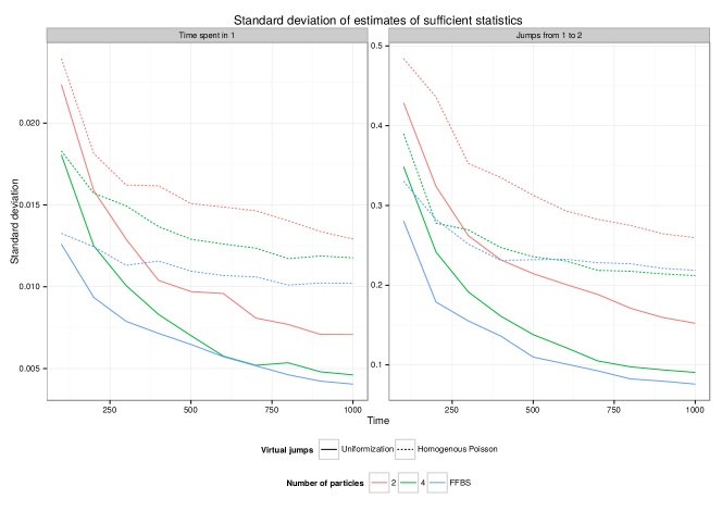
To analyze the rate of convergence of the algorithms we also compute standard deviation of sufficient statistics (number of jumps and time spent in each state). The results are shown in Figure 3. Again we obtain similar conclusions. It is clearly visible that the algorithms with FFBS have lower variance than those with PGAS. However, the difference is rapidly decreasing with increasing number of particles. Approximately the cost of FFBS is of order and the cost of PGAS is . Hence in the example under consideration, we obtain comparable quality of estimation for the algorithms with FFBS and PGAS which have the same computational cost.
8.2 Chain network
The model considered in this subsection is based on (Rao and Teh, 2013, Subsection 5.5). It is a network which consists of nodes equipped with the “chain” graph . For each node the set of possible states is . The transition intensities of every node, except the first one, depend on current state of the previous node. Namely, off-diagonal elements of intensity matrix are given by
In words, the head node leaves the current state with intensity and prefers to jump to . For any other node, if its current state differs from that of parent state then intensity of jumping is and the process prefers to jump to . If then the process leaves the current state with intensity and chooses a new state at random. We observe the process at the beginning and at the end of time interval .
We run two MCMC algorithms targeting the posterior distribution over latent trajectories. Our algorithm with PGAS based on particles is compared with Rao and Teh’s algorithm with FFBS. Both the algorithms use uniformization, with equal to twice the intensity of leaving the current state.
We begin with a network with nodes, states of every node and time length . In the first series of our experiments, we increase the number of nodes to . In the second series we increase the length of time interval to . Finally we change the size of the state space to . For each of the scenarios we run 20 replications of each of the MCMC algorithms. We use CODA R package (Plummer et al., 2006) to estimate the effective sample size of the following statistics: time spent in each state and number of jumps, for nodes . The median of all these quantities serves as an estimator of ESS for the whole CTBN.
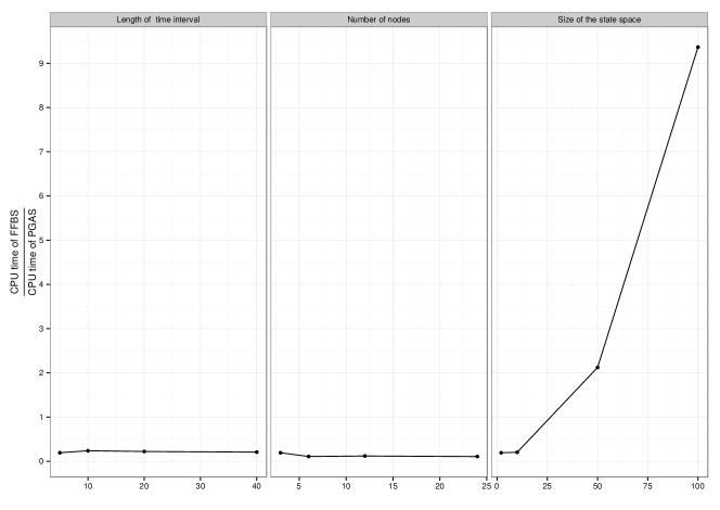
In Figure 4 we present the ratio of CPU time needed to generate a sample with ESS equal to . In the beginning, when state space is of size , FFBS is more effective, around 4-5 times as fast as PGAS. This is what should be expected, since the cost of PGAS with particles is higher than the cost of FFBS for a small space size. Also as expected, the ratio does not change significantly if the number of nodes increases. The same seems to happen if we increase the length of time interval. This last fact is slightly surprising, because the rate of convergence of particle Gibbs depends on the number of jumps, see Andrieu et al. (2013); Lindsten et al. (2014a). However, if the size of the state space increases then the cost of our proposed method becomess significantly lower than that of Rao and Teh (2013) approach. For instance if then our algorithm is twice as fast as Rao and Teh (2013) and for it is more than 9 times as fast. Experiments with a different number of particles () lead to the same conclusions.
8.3 Lotka-Volterra model

The last example is Lotka-Volterra model (Wilkinson, 2009; Opper and Sanguinetti, 2008), which describes evolution of two interacting populations of prey and predator species. This process can be viewed as the two node CTBN shown in Figure 5. Let and represent the size of prey and predator populations, respectively. The transition intensities are given by
All other intensities are . The state space is infinite: . Following Rao and Teh (2013) we set the parameters as follows: and . We condsider the process in time interval with known initial position and noisy observations at discrete times uniformly spaced in interval with the likelihood given by
Given this evidence, we estimate the posterior distribution over sample paths of using our sampler. We compute estimates of in the interval (where observations are available) and also predict values of in the interval . Due to unboudedness of intensities we are not able to use uniformization technique and so we use homogenous virtual jumps with . For this choice of , the number of virtual jumps is approximately equal to the number of true jumps. We run MCMC simulation of length with initial iterations treated as burn-in time. In the PGAS we use particles. The results of simulation are given in Figure 6.

We conclude that the quality of estimates is the same as in Rao and Teh (2013). Note that in opposition to Rao and Teh’s algorithm we need not truncate the state space and the computational cost of our algorithm is significantly lower, namely for our method and for Rao and Teh, with state space truncted to as suggested by these authors.
9 Conclusions
In the present paper we propose a new MCMC algorithm for sampling from the posterior distribution of hidden trajectory of a Markov jump process. The general idea is the same as in Rao and Teh (2013), namely we alternately add virtual jumps and update the skeleton of the process. The main novelty is that our algorithm uses PGAS to sample the skeleton, while Rao and Teh use FFBS. Thus instead of sampling exactly from a conditional distribution, we make a step of a Markov chain which preserves this distribution. This modification has some disadvantages, as slower mixing of the entire procedure. However, there are also important advantages of our approach. Unlike previous methods our algorithm can be implemented even if the state space is infinite. The cost of a single step of the proposed algorithm does not depend on the size of the state space. Consequently, we can recommend our algorithm for problems where the space is either infinite or finite but large. If the size of the state space is not big, then our algorithm with PGAS converges slightly slower than the algorithm with FFBS. However, the difference between them is rapidly diminishing if we increase the number of particles in PGAS.
In the present paper we describe an algorithm for time homogeneous processes, only to avoid too many technical details. However, the generalization to non-homogeneous processes is rather straightforward. For details of adding virtual jumps in non-homogeneous case we refer to Rao and Teh (2012). Since PGAS can easly deal with general state spaces, our algorithm can also be applied to piecewise deterministic Markov jump processes on general state spaces (i.e. processes which evolve deterministically between jumps and move according to some Markov kernel at moments of jumps).
We note that an important issue is to find an optimal number of virtual jumps. Small number of virtual jumps can lead to poor mixing of moments of jumps. In the case of PGAS, large number of virtual jumps not only increases computational cost, as it is in the case of FFBS, but may have a negative impact on mixing of the whole algorithm. It is because the convergence rate of particle Gibbs depends on the length of simulated trajectory.
Appendix A.
Proof [Proof of Proposition 1] We are to check that if has the distribution given by (3) then is distributed according to (2). First we compute the distribution of waiting time for the next true jump. Without loss of generality we can assume that the previous jump occurred at time and . To get the first true jump we generate subsequent moments of potential jumps such that are i.i.d. from . The candidate is accepted with probability . Hence
We have obtained an expression which is exactly the c.d.f. of waiting time for the next jump of process with intensity matrix . To conclude the proof, it is enough to note that
References
- Andrieu et al. (2010) Christophe Andrieu, Arnaud Doucet, and Roman Holenstein. Particle markov chain monte carlo methods. Journal of the Royal Statistical Society: Series B (Statistical Methodology), 72(3):269–342, 2010.
- Andrieu et al. (2013) Christophe Andrieu, Anthony Lee, and Matti Vihola. Uniform ergodicity of the iterated conditional smc and geometric ergodicity of particle gibbs samplers. arXiv preprint arXiv:1312.6432, 2013.
- Boys et al. (2008) Richard J Boys, Darren J Wilkinson, and Thomas BL Kirkwood. Bayesian inference for a discretely observed stochastic kinetic model. Statistics and Computing, 18(2):125–135, 2008.
- Chopin and Singh (to appear 2015) Nicolas Chopin and Sumeetpal S Singh. On the particle gibbs sampler. Bernoulli, to appear 2015.
- Cinlar (1975) Erhan Cinlar. Introduction to stochastic processes. Prentice-Hall, 1975. ISBN 0134980891.
- Cohn et al. (2010) Ido Cohn, Tal El-Hay, Nir Friedman, and Raz Kupferman. Mean field variational approximation for continuous-time bayesian networks. The Journal of Machine Learning Research, 11:2745–2783, 2010.
- Del Moral et al. (2006) Pierre Del Moral, Arnaud Doucet, and Ajay Jasra. Sequential monte carlo samplers. Journal of the Royal Statistical Society: Series B (Statistical Methodology), 68(3):411–436, 2006.
- Doucet and Johansen (2009) Arnaud Doucet and Adam M Johansen. A tutorial on particle filtering and smoothing: Fifteen years later. Handbook of Nonlinear Filtering, 12:656–704, 2009.
- Doucet et al. (2001) Arnaud Doucet, Nando De Freitas, and Neil Gordon. An introduction to sequential monte carlo methods. In Sequential Monte Carlo methods in practice, pages 3–14. Springer, 2001.
- Eddelbuettel et al. (2011) Dirk Eddelbuettel, Romain François, J Allaire, John Chambers, Douglas Bates, and Kevin Ushey. Rcpp: Seamless r and c++ integration. Journal of Statistical Software, 40(8):1–18, 2011.
- El-Hay et al. (2008) Tal El-Hay, Nil Friedman, and Raz Kupferman. Gibbs sampling in factorized continuous-time markov processes. In Proceedings of the Twenty-Fourth Conference Annual Conference on Uncertainty in Artificial Intelligence (UAI-08), pages 169–178, Corvallis, Oregon, 2008. AUAI Press.
- Fan and Shelton (2008) Yu Fan and Christian R. Shelton. Sampling for approximate inference in continuous time Bayesian networks. In Tenth International Symposium on Artificial Intelligence and Mathematics, 2008.
- Fan et al. (2010) Yu Fan, Jing Xu, and Christian R. Shelton. Importance sampling for continuous time Bayesian networks. Journal of Machine Learning Research, 11(Aug):2115–2140, 2010.
- Fearnhead and Sherlock (2006) Paul Fearnhead and Chris Sherlock. An exact gibbs sampler for the markov-modulated poisson process. Journal of the Royal Statistical Society: Series B (Statistical Methodology), 68(5):767–784, 2006. ISSN 1467-9868. doi: 10.1111/j.1467-9868.2006.00566.x.
- Hobolth and Stone (2009) Asger Hobolth and Eric A. Stone. Simulation from endpoint-conditioned, continuous-time markov chains on a finite state space, with applications to molecular evolution. The Annals of Applied Statistics, 3(3):1204–1231, 2009.
- Jensen (1953) Arne Jensen. Markoff chains as an aid in the study of markoff processes. Scandinavian Actuarial Journal, 1953(sup1):87–91, 1953.
- Lauritzen (2001) Steffen L Lauritzen. Causal inference from graphical models. Complex stochastic systems, pages 63–107, 2001.
- Lewis and Shedler (1979) P. A. W. Lewis and G. S. Shedler. Simulation of nonhomogeneous poisson processes with degree-two exponential polynomial rate function. Operations Research, 27(5):pp. 1026–1040, 1979.
- Lindsten and Schön (2013) Fredrik Lindsten and Thomas B Schön. Backward simulation methods for monte carlo statistical inference. Foundations and Trends in Machine Learning, 6(1):1–143, 2013.
- Lindsten et al. (2012) Fredrik Lindsten, Thomas Schön, and Michael I Jordan. Ancestor sampling for particle gibbs. In Advances in Neural Information Processing Systems, pages 2591–2599, 2012.
- Lindsten et al. (2014a) Fredrik Lindsten, Randal Douc, and Eric Moulines. Uniform ergodicity of the particle gibbs sampler. arXiv preprint arXiv:1401.0683, 2014a.
- Lindsten et al. (2014b) Fredrik Lindsten, Michael I Jordan, and Thomas B Schön. Particle gibbs with ancestor sampling. The Journal of Machine Learning Research, 15(1):2145–2184, 2014b.
- Miasojedow et al. (2014) Blazej Miasojedow, Wojciech Niemiro, John Noble, and Krzysztof Opalski. Metropolis-type algorithms for continuous time bayesian networks. arXiv preprint arXiv:1403.4035, 2014.
- Nodelman et al. (2002a) Uri Nodelman, Christian R Shelton, and Daphne Koller. Continuous time bayesian networks. In Proceedings of the Eighteenth conference on Uncertainty in artificial intelligence, pages 378–387, 2002a.
- Nodelman et al. (2002b) Uri Nodelman, Christian R Shelton, and Daphne Koller. Learning continuous time bayesian networks. In Proceedings of the Nineteenth conference on Uncertainty in Artificial Intelligence, pages 451–458. Morgan Kaufmann Publishers Inc., 2002b.
- Nodelman et al. (2005) Uri Nodelman, Daphne Koller, and Christian R Shelton. Expectation propagation for continuous time bayesian networks. In Proceedings of the Twenty-first Conference on Uncertainty in AI (UAI), pages 431–440, Edinburgh, Scottland, UK, July 2005.
- Norris (1998) James R Norris. Markov chains. Number 2. Cambridge university press, 1998.
- Opper and Sanguinetti (2008) Manfred Opper and Guido Sanguinetti. Variational inference for markov jump processes. In Advances in Neural Information Processing Systems, pages 1105–1112, 2008.
- Pitt and Shephard (1999) Michael K Pitt and Neil Shephard. Filtering via simulation: Auxiliary particle filters. Journal of the American statistical association, 94(446):590–599, 1999.
- Plummer et al. (2006) Martyn Plummer, Nicky Best, Kate Cowles, and Karen Vines. Coda: Convergence diagnosis and output analysis for mcmc. R News, 6(1):7–11, 2006.
- Rao and Teh (2012) Vinayak Rao and Yee W Teh. Mcmc for continuous-time discrete-state systems. In Advances in Neural Information Processing Systems, pages 701–709, 2012.
- Rao and Teh (2013) Vinayak Rao and Yee W Teh. Fast MCMC sampling for Markov jump processes and extensions. Journal of Machine Learning Research, 14:3207–3232, 2013.
- Roberts and Rosenthal (2004) Gareth O Roberts and Jeffrey S Rosenthal. General state space markov chains and mcmc algorithms. Probability Surveys, 1:20–71, 2004.
- Schweder (1970) Tore Schweder. Composable markov processes. Journal of applied probability, 7(2):400–410, 1970.
- Wilkinson (2009) Darren J Wilkinson. Stochastic modelling for quantitative description of heterogeneous biological systems. Nature Reviews Genetics, 10(2):122–133, 2009.