Understanding AGB evolution in Galactic bulge stars from high-resolution infrared spectroscopy

Abstract

An analysis of high-resolution near-infrared spectra of a sample of 45 asymptotic giant branch (AGB) stars towards the Galactic bulge is presented. The sample consists of two subsamples, a larger one in the inner and intermediate bulge, and a smaller one in the outer bulge. The data are analysed with the help of hydrostatic model atmospheres and spectral synthesis. We derive the radial velocity of all stars, and the atmospheric chemical mix ([Fe/H], C/O, ¹²C/¹³C, Al, Si, Ti, and Y) where possible. Our ability to model the spectra is mainly limited by the (in)completeness of atomic and molecular line lists, at least for temperatures down to $T_{\rm eff}\approx 3100$ K. We find that the subsample in the inner and intermediate bulge is quite homogeneous, with a slightly sub-solar mean metallicity and only few stars with super-solar metallicity, in agreement with previous studies of non-variable M-type giants in the bulge. All sample stars are oxygen-rich, C/O$<$1.0. The C/O and carbon isotopic ratios suggest that third dredge-up (3DUP) is absent among the sample stars, except for two stars in the outer bulge that are known to contain technetium. These stars are also more metal-poor than the stars in the intermediate or inner bulge. Current stellar masses are determined from linear pulsation models. The masses, metallicities and 3DUP behaviour are compared to AGB evolutionary models. We conclude that these models are partly in conflict with our observations. Furthermore, we conclude that the stars in the inner and intermediate bulge belong to a more metal-rich population that follows bar-like kinematics, whereas the stars in the outer bulge belong to the metal-poor, spheroidal bulge population.

1 Introduction

The Galactic bulge is a complex structure in the central regions of the Milky Way Galaxy. Its stellar populations have been studied in some detail in the recent years. Stellar types that have been investigated by high-resolution spectroscopy in the past range from microlensed dwarf and subgiant stars (Bensby et al., 2013, and references therein), to K-type giants (e.g. Babusiaux et al., 2010; Hill et al., 2011; Uttenthaler et al., 2012; Ness et al., 2013), to M-type giants (Rich et al., 2012, and references therein). Also planetary nebulae (PNe) in the bulge have been studied spectroscopically (Maciel, 1999; Chiappini et al., 2009; Guzman-Ramirez et al., 2011).

A group of bulge stars that has so far not been studied in detail by high-resolution spectroscopy consist of the asymptotic giant branch (AGB) stars. AGB stars represent the last stage of stellar evolution where the energy output is dominated by nuclear burning. This stage is characterised by strong pulsations of the envelope that enhance the stellar wind, which is accelerated by radiation pressure acting on dust particles formed in the outflowing material. Eventually, the stellar evolution is terminated by the high mass loss and the star may enter the PN phase. In the deep interior of the star, nucleosynthetic processes take place that produce carbon (¹²C) and heavy elements. These may subsequently be brought to the surface by a deep mixing event called the third dredge-up (3DUP). If enough C is added to the atmosphere, the abundance ratio of C to O (by number of atoms) will exceed 1.0 and the star will become a carbon star (C-star). The formation of C-stars depends on the initial mass and metallicity: A star may turn into a C-star only if it is massive enough to undergo enough 3DUP events, where the lower mass limit is a function of metallicity, being lower for lower metallicity (Marigo et al., 2013; Karakas, 2014). The lack of C-stars in the inner regions of M31 (Boyer et al., 2013) suggests that there could be a metallicity threshold above which the formation of C-stars is inhibited altogether.

AGB stars in the Galactic bulge are interesting for a number of reasons. First of all, it has been shown that intrinsic carbon stars, i.e. stars that owe their enhancement of C to internal nucleosynthesis and 3DUP and not to binary mass transfer, are widely absent in the Galactic bulge (Azzopardi et al., 1996; Blanco & Terndrup, 1989; Tyson & Rich, 1991; Ng, 1997; Schultheis, 1998). This would mean that either the mass of bulge stars is too low or the metallicity too high to undergo (sufficient) 3DUP to form C-stars. However, it is known that oxygen-rich AGB stars in the outer Galactic bulge show absorption lines of technetium (Tc), a clear indicator of recent or ongoing 3DUP (Uttenthaler et al., 2007). This suggests that 3DUP does happen in bulge stars, but probably not enough to form C-stars. An exception may be the first carbon Mira in the direction of the Galactic bulge that was recently presented by Miszalski et al. (2013). It is not clear if that star is indeed a member of the Galactic bulge.

Samples of non-variable M-type giants, the precursors of variable AGB stars, have been studied by Rich & Origlia (2005), Rich et al. (2007), and Rich et al. (2012). One of their main results is that the mean metallicity of M-giants in the bulge is slightly sub-solar, and that stars with super-solar metallicity are not common. On the other hand, it was concluded by Buell (2013) that PNe in the Galactic bulge, the evolutionary successors of AGB stars, have a relatively high, i.e. on average super-solar, metallicity. Yet again, Uttenthaler et al. (2012) suggests that AGB stars in the outer bulge predominantly descend from the metal-poor population ($[{\rm Fe}/{\rm H}]\approx-0.6$), not from the metal-rich population ($[{\rm Fe}/{\rm H}]\approx+0.3$) of the bulge. This latter result was derived from the fact that the radial velocity dispersion of AGB stars and also of PNe in the outer bulge is similar to that of the metal-poor population, which differs significantly from that of the metal-rich population.

Finally, Perea-Calderón et al. (2009) and Guzman-Ramirez et al. (2011) showed that many Galactic bulge PNe exhibit evidence of mixed chemistry with emission from both silicate dust and polycyclic aromatic hydrocarbons (PAHs), the latter being a signature of C-rich chemistry. Such signatures are difficult to explain in an environment with (assumed) low C/O ratio, which required Guzman-Ramirez et al. (2011) to invoke hydrocarbon chemistry in an UV-irradiated, dense torus around the central stars of the PNe. In their chemical model, the formation of PAHs would be considerably eased if the C/O ratio was increased from its initial value by at least a few 3DUP events.

These considerations make Galactic bulge AGB stars interesting targets for further investigation. A determination of the metallicity and mass of AGB stars would help in understanding the lack of intrinsic C-stars in the bulge. In particular, a metallicity determination would shed light on the discrepancies in the metallicities of non-variable M-type giants and PNe in the bulge. A measurement of the C/O ratio in bulge AGB stars would provide observational constraints to explanations for the mixed-chemistry phenomenon in Galactic bulge PNe.

In this paper we present near-IR spectroscopic observations of such a sample of stars and the chemical composition derived from them. The near-IR range has a number of advantages over the optical spectral range for studies of bulge red giants, most of all the lower interstellar extinction, less crowding of lines, and smaller effects of departures from local thermodynamic equilibrium (see Ryde et al., 2009, for a detailed discussion). Also 3D effects are smaller in the near-IR than in the optical range (Kučinskas et al., 2013). Thus, with these data, abundance determinations are done that would not be possible to obtain from optical spectra, as used e.g. in Uttenthaler et al. (2007).

The paper is organised as follows: The sample selection, observations, and data reduction are presented in Sect. 2, the analysis of that data is described in Sect. 3; the results and their discussion are to be found in Sect. 4; and conclusions are drawn in Sect. 5.

2 Sample selection, observations, and data reduction

In order to study the dust formation in the circumstellar environment of AGB stars, a mid-infrared spectroscopic survey with the IRS spectrograph (Houck et al., 2004) on board the Spitzer space telescope was performed on a sample of Galactic bulge AGB stars (Spitzer Proposal ID #3167, PI J. Blommaert; Blommaert et al., 2007; Vanhollebeke, 2007; Golriz et al., 2014). The targets for that survey were selected from the ISOGAL survey (Omont et al., 2003) in intermediate bulge fields ($|b|=1\degr$ to $4\degr$, corresponding distance from the mid-plane $\sim 140-560$ pc at $R_{0}=8.0$ kpc). The $(K_{\rm S}-[15])$ colour, where [15] is the 15 $\mu$m band of the ISO satellite, is an estimate of the dust mass-loss rate of the stars (Ojha et al., 2003; Blommaert et al., 2006) and was used to ensure that the full range of mass-loss rates, starting from the onset of (dust) mass loss up to the mass-loss rates of the so-called super-winds of OH/IR stars ($10^{-4}M_{\sun}/{\rm yr}$) was included in the sample.

We selected from this Spitzer IRS sample those stars for high-resolution near-IR observations for which we expected to be able to model their near-IR spectra, i.e. OH/IR stars were excluded. Nevertheless, four large-amplitude variables (LAVs) were observed. Following the recommendations of McSaveney et al. (2007), these four LAVs were selected such that they would be near minimum light at the time of the observing run. The initial goal of the observations was to determine the C/O and ¹²C/¹³C ratios of the stars as an “evolutionary clock” along the AGB as a result of repeated 3DUP. The observations were carried out in visitor mode (observer: J. Blommaert) with the CRyogenic high-resolution InfraRed Echelle Spectrograph (CRIRES Käufl et al., 2004) in three nights between 09 and 12 June 2008. The target stars themselves were used as guide star for the wave-front sensor of the adaptive optics system. An entrance slit width of 0.4″was chosen, which results in a nominal resolving power of $R=\lambda/\Delta\lambda=50\,000$.

Along with the 37 bulge AGB stars from the Spitzer sample, spectra were also obtained of a few comparison stars that had been studied previously with high-resolution near-IR spectroscopy by other authors. These include BMB 78 studied by Cunha & Smith (2006), BD$-$012971, which was studied by Rich & Origlia (2005), as well as BMB 289, which was investigated by both these works. Furthermore, spectra of five K/M-type field giants were obtained; the analysis and results for the field stars are reported in the Appendix.

Also included in the present paper is an analysis of CRIRES spectra of eight AGB stars in the outer bulge, the so-called Plaut stars (Plaut, 1971). They are much further from the Galactic mid-plane than the Spitzer stars, at $b\sim-10\degr$ or $\sim 1.4$ kpc. These stars were selected from the sample discussed in Uttenthaler et al. (2007) and include all four stars that were found to contain Tc in their atmosphere, as well as four Tc-poor stars. These observations were done either in the science verification runs (August 2006) or in a regular service mode observing programme (Prog. ID 383.D-0685(A), September 2009).

All stars were observed at least in one setting in the H-band (grating order 36) and in the K-band (grating order 24). The H-band spectra cover approximately the range $\lambda_{\rm vac}\simeq 1543$ to 1561 nm, with a gap of $\sim 2$ nm between the detectors. Due to contamination from neighbouring orders, only data from detector chips 2 and 3 are considered here. The H-band spectra are dominated by the ¹²CO 3-0 band head, a number of OH and CN lines, as well as atomic lines (Fe, Ni, Si, Ti, S). The K-band spectra in grating order 24 cover the range $\lambda_{\rm vac}\simeq 2355$ to 2407 nm and are dominated by CO $\Delta\nu=2$ lines.

Sixteen of the science targets and one of the comparison stars were observed in two additional settings in the K-band to also have lines available of atomic species that are relevant for the dust formation. These spectra in the grating orders 27 and 26 cover the range $\lambda_{\rm vac}\simeq 2087$ to 2134 nm and 2174 – 2222 nm, respectively. Besides being cluttered with abundant CN lines, these spectra contain, amongst others, lines of Na, Mg, Al, Si, Sc, Ti, and Fe. The Na lines were targeted to check a possible correlation between Na line equivalent width measured from low-resolution spectra and dust mineralogy in the circumstellar envelope. This correlation was not reproduced with the high-resolution spectra.

A basic reduction of the data was done with the standard ESO CRIRES pipeline, version 1.7.0. Further processing, in particular wavelength calibration and telluric correction, was done with custom-made IDL tools. The H-band spectra were wavelength-calibrated manually using the ThAr lamp exposures taken at day time. Due to the lack of suitable ThAr lines in the K-band settings, these spectra were wavelength-calibrated using the numerous telluric features imprinted in them.

Before dividing the science target spectrum by the telluric standard star spectrum for telluric correction, both spectra were re-binned to a common wavelength vector and the airmass of the telluric spectrum was adjusted to that of the corresponding science spectrum according to the Lambert-Beer law:

$$f_{\rm std,adj}=\exp\left[\ln\left(f_{\rm std}\right)\frac{X_{\rm sci}}{X_{\rm std}}\right],$$

with $f_{\rm std}$ the flux of the telluric standard star spectrum continuum-normalised to 1.0, and $X_{\rm{sci}}$ and $X_{\rm{std}}$ the airmass of the science target and of the telluric standard star, respectively. The science spectrum was then divided by the adjusted standard star spectrum. This careful procedure in the telluric correction yielded very satisfactory results. Weak residuals from the division were only discernible in the cores of the strongest telluric lines. No telluric correction was applied to the H-band spectra because the wavelength range under consideration is essentially free from telluric absorption. The achieved signal-to-noise ratio (S/N) per pixel of the reduced one-dimensional spectra is relatively high ($\sim 100$) for most stars, only for a few stars it is somewhat low (of the order of 30). The S/N is thus not the limiting factor in the analysis of most stars.

Particular care was taken in the final step of data reduction, the continuum normalisation. The prime method used in this step was to identify narrow pieces of spectrum (a few 0.01 up to 0.10 nm) that are basically unaffected by line absorption in as many of the sample stars as possible. The mean flux of the 30% brightest pixels in these ranges was set to define the continuum (flux=1.0). This continuum placement was always checked in comparison with synthetic spectra. Figure 5 provides an example of how well the continuum in observed and synthetic spectra are matched. In some cases, in particular for the coolest and most strongly variable stars, even these narrow pieces of spectrum were affected by line absorption. In these cases, the continuum was placed manually, mostly by dividing it by its maximum flux, except in cases that were obviously affected by bad pixels, residuals of the telluric correction, or emission components. This method was necessary anyway in the K-band spectra of grating order 24 because this spectral region is heavily cluttered with CO $\Delta\nu=2$ lines.

3 Analysis

3.1 Stellar parameter determination

Before determining elemental abundances from the high-resolution spectra using spectral synthesis techniques, the main physical parameters of our sample stars need to be determined. We derived those stellar parameters from low-resolution optical spectra, broad band photometry, and the pulsation periods of the stars. These data will be described in more detail in a separate paper (Vanhollebeke et al., in preparation).

3.1.1 Pulsation period

The pulsation periods of the sample stars are an important ingredient for the stellar parameter determination. K-band photometry of the Spitzer sub-sample spanning $\sim 820$ days was obtained by one of us (PW) and analysed by Vanhollebeke (2007), who also derived pulsation periods where possible. Furthermore, the VizieR database was searched for additional period determinations. The Optical Gravitational Lensing Experiment (OGLE)-II catalogue provided pulsation periods for a few more objects, in particular among the short-period, low-amplitude variables. In cases where two periods were available, the one from Vanhollebeke (2007) was adopted. For the Plaut stars, the periods and K-band magnitudes were taken from Uttenthaler et al. (2007) and Uttenthaler et al. (2008). The mean K-band magnitudes and adopted periods are listed in columns 4 and 5, respectively, of Table 1.

Table 1: Main parameters of the sample stars. Meaning of the columns: object name; Galactic longitude $l$; Galactic latitude $b$; mean K-band magnitude; pulsation period; adopted effective temperature; luminosity derived by integrating the SED; luminosity corrected for bulge depth scatter using the period – K-magnitude relations of Ita et al. (2004, see Sect. 3.1.3); current pulsation mass; adopted $\log g$ of the model atmosphere used in the analysis (see Sect. 3.1.4); LAV: large-amplitude variable. Unknown values are replaced by ’…’. The luminosities of the comparison stars BMB 78, BMB 289, and BD$-$012971 are calculated from their temperatures and surface gravities, assuming 1 $M_{\sun}$.

Object name	$l$	$b$	$\left<K\right>$	Period	$T_{\rm eff}$	$L_{\star}/L_{\sun}$	$L_{\star}/L_{\sun}$	$M/M_{\sun}$	$\log g$	Remark
	[deg]	[deg]	(mag)	(days)	(K)	uncorr.	corr.		cgs
BMB 78a	1.15	$-3.78$	7.53	…	3600	654	…	…	0.80
BMB 289a	1.22	$-4.02$	6.17	…	3375	1268	…	…	0.40
BMB 289b			6.17	…	3200	814	…	…	0.50
BD$-$012971b	$-11.5$	50.8	4.29	…	3600	1304	…	…	0.50
J174117.5-282957	$-0.13$	1.04	7.10	…	2800	5609	…	…	$-0.28$
J174123.6-282723	$-0.08$	1.04	8.32	…	3200	1638	…	…	0.13
J174127.3-282851	$-0.09$	1.02	7.26	438.95	2600	4732	…	1.85	$-0.26$	LAV
J174127.9-282816	$-0.08$	1.02	7.14	…	3000	4921	…	…	$-0.20$
J174128.5-282733	$-0.07$	1.02	7.48	309.46	3000	3652	4804	1.37	$-0.20$
J174139.5-282428	$-0.01$	1.02	7.04	…	2800	5314	…	…	$-0.28$
J174140.0-282521	$-0.02$	1.01	7.26	…	2900	4813	…	…	$-0.20$
J174155.3-281638	0.14	1.04	6.82	…	2700	6324	…	…	$-0.28$
J174157.6-282237	0.06	0.98	7.58	…	3300	3342	…	…	$-0.13$
J174203.7-281729	0.14	1.00	7.55	392.12	2800	4541	…	1.38	$-0.23$	LAV
J174206.9-281832	0.13	0.98	7.26	481.61	2800	5152	…	1.29	$-0.28$	LAV
J174917.0-293502	$-0.14$	$-1.02$	8.55	…	3200	1541	…	…	0.16
J174924.1-293522	$-0.13$	$-1.04$	8.54	…	3700	1680	…	…	0.37
J174943.7-292154	0.10	$-0.99$	7.94	…	3000	2413	…	…	$-0.15$
J174951.7-292108	0.12	$-1.01$	8.26	…	3500	1795	…	…	0.25
J175432.0-295326	0.18	$-2.16$	7.29	401.74	2900	3844	…	0.94	$-0.20$
J175456.8-294157	0.39	$-2.14$	6.90	322.11	2900	5699	5410	1.82	$-0.23$
J175459.0-294701	0.32	$-2.19$	6.96	472.15	2600	6095	…	2.38	$-0.26$	LAV
J175515.4-294122	0.43	$-2.19$	8.26	76.90	3300	1652	2059	0.69	0.00
J175517.0-294131	0.43	$-2.20$	7.99	…	3500	2483	…	…	0.11
J180238.8-295954	0.96	$-3.73$	7.86	119.00	3200	2005	3843	0.92	$-0.21$
J180248.9-295430	1.05	$-3.72$	8.13	75.69	3300	1759	2116	0.68	0.00
J180249.5-295853	0.99	$-3.76$	8.65	65.18	3400	1214	1848	0.73	0.12
J180259.6-300254	0.95	$-3.82$	7.46	228.87	3000	2971	3374	1.22	$-0.14$
J180301.6-300001	1.00	$-3.81$	8.37	33.51	3400	1330	606	0.45	0.38
J180304.8-295258	1.10	$-3.76$	8.53	35.52	3400	1147	683	0.48	0.38
J180305.3-295515	1.07	$-3.78$	7.15	207.02	3100	4023	2944	1.02	$-0.10$
J180305.4-295527	1.07	$-3.78$	8.00	113.94	3200	2015	4184	1.15	$-0.14$
J180308.2-295747	1.04	$-3.81$	7.92	113.04	2800	1919	3613	2.13	$-0.04$
J180308.7-295220	1.12	$-3.77$	7.94	98.00	3100	1782	2842	1.04	$-0.07$
J180311.5-295747	1.05	$-3.82$	7.39	292.04	2900	3036	4557	1.64	$-0.20$
J180313.9-295621	1.07	$-3.82$	8.04	75.00	3400	1801	2073	0.61	0.05
J180316.1-295538	1.09	$-3.82$	8.31	62.69	3300	1328	1519	0.65	0.13
J180323.9-295410	1.12	$-3.83$	8.15	84.84	3200	1547	2409	0.82	$-0.05$
J180328.4-295545	1.11	$-3.86$	7.40	119.09	3200	3005	3850	1.15	$-0.11$
J180333.3-295911	1.06	$-3.90$	8.44	203.95	3300	1247	2970	0.78	$-0.11$
J180334.1-295958	1.05	$-3.91$	7.06	119.09	3100	3986	3696	1.06	$-0.18$
Plaut 3-45	$-0.94$	$-7.22$	6.65	271.02	3000	5308	3938	1.25	$-0.19$	LAV
Plaut 3-100	$-3.85$	$-8.92$	6.37	298.70	3000	8288	5432	1.68	$-0.21$	LAV
Plaut 3-315	0.04	$-7.65$	6.54	326.80	3100	6351	5514	1.30	$-0.27$	LAV
Plaut 3-626	$-2.63$	$-10.10$	7.19	298.48	3400	3835	5344	0.89	$-0.26$	LAV, Tc-rich
Plaut 3-794	0.92	$-9.03$	6.04	303.54	3000	11278	5584	1.71	$-0.21$	LAV
Plaut 3-942	$-2.41$	$-11.47$	6.55	338.00	3500	6753	6235	0.83	$-0.31$	LAV, Tc-rich
Plaut 3-1147	$-1.84$	$-12.31$	5.77	395.63	3000	13506	7577	1.84	$-0.31$	LAV, Tc-rich
Plaut 3-1347	0.35	$-12.60$	5.99	426.60	3300	10730	8143	1.16	$-0.38$	LAV, Tc-rich

3.1.2 Temperature

The most important stellar parameter for our spectroscopic analysis is the effective temperature. To this end, low-resolution flux-calibrated optical spectra were obtained by one of us (PW) with the Double-Beam Spectrograph (DBS) mounted to the Australian National University 2.3 m telescope at Siding Spring Observatory (Australia). More information on the instrument can be found in Rodgers et al. (1988). Exposure times ranged between 200 and 1200 s. The precise wavelength range of the optical spectra varies, but the part between 666 – 1000 nm is always covered. This range includes prominent TiO and VO bands that are very sensitive to the effective temperature of the star (see e.g. Reiners, 2005). Furthermore, the general slope of the spectra can constrain the star’s temperature.

For the Spitzer sample stars identified as non-variable by Vanhollebeke (2007, Sect. 3.1.1), low-resolution spectra that were obtained several years before the CRIRES run were used. These older spectra have a dispersion of 0.41 nm/pixel. The sample stars identified as variable were observed with the DBS between 16 and 18 days after the CRIRES run in which the Spitzer sub-sample was observed. These spectra have a somewhat higher resolution of 0.187 nm/pixel. We may safely assume that the temperature derived from the optical spectra is representative for the temperature at the time of the CRIRES observations: stars with short pulsation periods and low amplitudes do not exhibit a large temperature change over a pulsation cycle, while for the stars with longer periods and larger amplitudes the time delay between CRIRES and DBS observations is small compared to the pulsation period. For the Plaut stars, the CRIRES and DBS observations were done at independent phases, hence here the temperature determined from the low-resolution spectra may deviate somewhat more from that at the actual time of CRIRES observations. All sample stars were identified to be oxygen-rich from the low-resolution spectra, i.e. they all exhibit the characteristic TiO bands. Also the Tc-rich stars have very prominent TiO bands, the ZrO bands are present but not dominant. In the observed spectral range, C-stars would be identified by intense bands of the CN molecule.

Before temperature determination, the optical low-resolution spectra were corrected for interstellar reddening. The same extinction values as in Vanhollebeke (2007) were adopted, which stem from the maps of Schultheis et al. (1999), Sumi (2004), and Marshall et al. (2006). These values were applied to establish the extinction as a function of wavelength, using the relations given in O’Donnell (1994) and Cardelli et al. (1989). The spectra were divided by this extinction curve to obtain the de-reddened spectrum. Test runs show that the resulting temperatures are quite insensitive to the extinction value.

The main method to derive temperatures from the optical spectra involves fitting of series of model spectra to the observed spectra. A series of COMARCS model atmospheres and spectra (see Sect. 3.2) was calculated, with temperatures between 2600 and 3800 K in steps of 100 K, $\log g\,[{\rm cm\,s^{-2}}]=0.0$, 1 M_☉, microturbulence 3 km s^-1, solar C/O ratio, and two metallicities: 1.0 Z_☉ and 0.3 Z_☉. Extensive lists of atomic and molecular lines, in particular of TiO and VO, were taken into account in the calculation of the spectra. In addition, we used a grid of PHOENIX model spectra (Husser et al., 2013) with temperatures between 2000 and 3900 K in steps of 100 K, solar metallicity, and otherwise identical parameters as the COMARCS grid. We fitted the model spectra to the observed spectra with a modified $\chi^{2}$ method in the form

$$\chi=\frac{1}{N}\sum_{i=1}^{N}\frac{\sqrt{\left(f_{{\rm obs},i}-f_{{\rm model},i}([{\rm Fe}/{\rm H}])\right)^{2}}}{\frac{1}{2}\left(f_{{\rm obs},i}+f_{{\rm model},i}([{\rm Fe}/{\rm H}])\right)}.$$

The wavelength range between 700 and 930 nm was used to find the temperature at which the model spectra best fit an observed spectrum. The lower wavelength limit was chosen to avoid the noise-dominated blue part of the observed spectrum, whereas the upper limit was chosen to avoid a molecular band of ZrO that might be present in the stars that had experienced 3DUP but not in stars that had not. This band could potentially have a systematic impact on the derived temperature. For the non-variable stars in the sample, the $(V-K)_{0}$ vs. $T_{\rm eff}$ calibration of van Belle et al. (1999) was used to derive another temperature estimate. This photometric temperature estimate agrees well with that derived from fitting the optical spectra. The final adopted temperature listed in column 6 of Table 1 was chosen based on a visual inspection of the observed spectra and of the model fits to them. We also tried to derive temperatures from the spectral parameters defined in Fluks et al. (1994, their Eq. 17 – 19), but found that these estimates sometimes vary considerable for a given star. The narrow bandpasses lie at the bottom of molecular bands that are formed in the very outer layers of the star, which are most affected by dynamic effects (pulsation, mass loss).

The determined temperature may depend on the adopted metallicity of the model spectra. Conversely, the metallicity that we derive from the high-resolution spectra depends on the model input temperature. An independent determination of effective temperature and metallicity without any assumptions is very difficult for our sample stars. In the above procedure we find relatively modest differences between the temperatures derived using the models with 1.0 Z_☉ and 0.3 Z_☉, respectively. The impact of the assumption on the metallicity for temperature determination seems limited and we are thus confident that we can derive reliable abundances from the high-resolution spectra. In any case, the CO lines are quite insensitive to the effective temperature.

3.1.3 Luminosity

The luminosity of each sample star was determined by integrating its spectral energy distribution (SED). To construct the SED, we collected I-band photometry from the DENIS catalogue (Epchtein et al., 1997), cycle-averaged J, H, K, L_nb band photometry from Wood et al. (1998) and Vanhollebeke (2007), Spitzer IRAC and MIPS 24 photometry (Uttenthaler et al., 2010; Hinz et al., 2009), as well as photometry from the WISE (Wright et al., 2010), ISOGAL (Omont et al., 2003), Akari (Ishihara et al., 2010), and MSX (Egan et al., 2003) surveys. Because for most stars the bulk of the stellar flux is emitted between the J and L bands and because cycle-averaged fluxes in these bands are used, we are confident to have very precise luminosities at hand for our sample stars. The photometry was de-reddened for interstellar extinction (see Sect. 3.1.2) and converted to flux values (Jansky). The whole SED was integrated numerically by connecting the data points by straight lines, and an extrapolation to the origin $(\nu,f)=(0,0)$ was included. To convert this apparent flux to a luminosity in solar units, a distance modulus of 14$\aas@@fstack{m}$5, corresponding to a distance of 8.0 kpc to the bulge, was assumed. A typical example of a de-reddened SED is shown in Fig. 1.

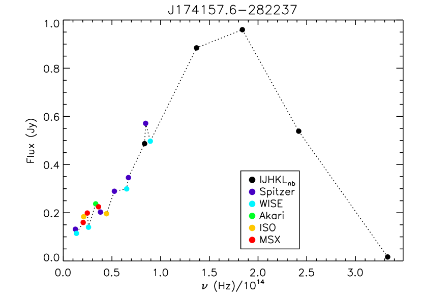
Figure 1: Typical example of a de-reddened SED of a sample star (J174157.6-282237). The source of the various data points is indicated in the legend. The luminosity of this star was found to be 3342 $L_{\sun}$.

For stars with a measured pulsation period, we corrected these luminosities by forcing them to fall on one of the period – K-magnitude relations of Ita et al. (2004), in an attempt to correct for the distance scatter within the bulge (red points in Fig. 3). A difference in the distance modulus between the Large Magellanic Cloud and the bulge of 4$\aas@@fstack{m}$0 was assumed. A $\log P-K_{0}$ diagram (Fig. 2) reveals that the long period stars probably follow sequence C (fundamental mode or Mira-like pulsators), whereas the shorter period stars probably follow sequence C’ (first overtone or semi-regular pulsators). We assume that the transition occurs at a period of 160 d ($\log(P)\sim 2.2$). Both the uncorrected and corrected luminosities are listed in columns 7 and 8 of Table 1.

Figure 2: $\log P-K_{0}$ diagram of our sample stars. Black symbols are the Spitzer sample stars, filled red diamonds the Tc-rich Plaut stars, open red diamonds the Tc-poor Plaut stars. The solid lines are the relations C (fundamental mode pulsators) and C’ (first overtone pulsators) from Ita et al. (2004).

This correction would lead to very high luminosities (8000 $L_{\sun}$ and more) and subsequently unrealistically high current masses ($3-5M_{\sun}$, see next Section) for the five Spitzer sample stars with the longest pulsation periods, four of them being the LAVs. Because their very red $(J-K)_{0}$ colours (up to 2.29) and considerable mid-IR excesses suggest that their K-band magnitudes are diminished by strong circumstellar extinction (cf. Fig. 20 in Vassiliadis & Wood, 1993) we did not apply the distance correction to their luminosities. The long-period Plaut stars do not show such extreme colours, which is why the correction was applied nevertheless.

The Plaut stars preferentially lie above sequence C in Fig. 2, whereas the Spitzer stars seem to lie preferentially below the sequences. The location of the Plaut stars can be understood as a result of selection effects that favoured stars on the near side of the bulge. They were discovered by photographic plate photometry (Plaut, 1971) and selected for optical spectroscopy (Uttenthaler et al., 2007). The location of the Spitzer stars is more surprising, at the moment we do not have a convincing explanation why they are preferentially at distances farther than the Galactic centre.

Figure 3 shows a Hertzsprung-Russell diagram with inverted temperature axis of the sample stars. The solid blue line in that figure is an isochrone from Bressan et al. (2012) with 5.0 Gyr age, $Z=0.017$ (solar metallicity), and including dust formation on the AGB. Stars on the AGB of this isochrone have a current mass of $\sim 1.29M_{\sun}$. The RGB tip of this isochrone is at $\sim 2500L_{\sun}$. Most of the sample stars define a clear trend of increasing luminosity with decreasing temperature, as may be expected from stars distributed along the AGB. Because temperature and luminosity of the stars were derived from completely independent data, it can be excluded that a systematic effect produces such a trend. The isochrone covers well the distribution of of our sample stars and reproduces the trend of increasing luminosity with decreasing temperature. The Tc-rich Plaut stars are shifted away from the isochrone to somewhat higher temperature and/or higher luminosity. At lower metallicity, stars on the AGB have higher temperatures at a given luminosity. As will be shown later, the two Tc-rich stars for which we are able to determine the metallicity are relatively metal-poor. This could explain their displacement from the location of the other stars.

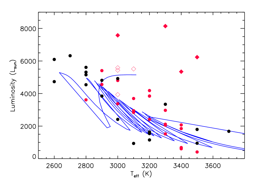
Figure 3: Luminosity vs. effective temperature diagram of the sample stars. Stars whose luminosities were not corrected for the bulge depth scatter due to the lack of a known pulsation period are plotted as black symbols, those whose luminosities were corrected are plotted as red symbols. The Plaut stars are plotted with the same symbols as in Fig. 2. The blue graph is an isochrone from Bressan et al. (2012) with 5.0 Gyr age, solar metallicity, and including dust formation on the AGB.

3.1.4 Current mass and surface gravity

Current pulsation masses for the variable stars with a determined period were computed. The linear pulsation models used here have been applied to LMC cluster variables, where they yield masses that are in good agreement with those expected from the cluster ages determined by main-sequence turn-off fitting (Kamath et al., 2010). Linear pulsation periods were computed with the code described in Lebzelter & Wood (2007), except that the low temperature opacities were generated from the web site described in Marigo & Aringer (2009). Metal and helium mass fractions of $Z=0.016$ and $Y=0.28$ were used. A grid of AGB models with $600<L/L_{\sun}<10\,000$ and $0.7<M/M_{\sun}<5.0$ was made and the linear fundamental and first overtone periods calculated. Analytic fits to the models were made in the form

$$\log\frac{M}{M_{\sun}}=0.324-1.699p+3.050r+1.007p^{2}+1.891r^{2}-2.515pr$$

and

$$\log\frac{M}{M_{\sun}}=-0.143-2.148p+3.271r-0.687p^{2}-0.894r^{2}+1.524pr$$

for the fundamental and first overtone modes, respectively, where $p=\log P-2$ and $r=0.5\left(\log L/L_{\sun}-4\log T_{\rm eff}\right)+5.3$. These fits to the pulsation mass are accurate to better than 7% for all computed models. Stars with $L/L_{\sun}<2000$ could be RGB stars rather than AGB stars. Similar fits were made to RGB models with luminosities $600<L/L_{\sun}<2000$ and $0.6<M/M_{\sun}<1.0$, the difference between the AGB and RGB models being the core mass. The core masses for the AGB models were assumed to be given by the formula in Wood & Zarro (1981) while RGB masses were obtained from the stellar models of Girardi et al. (2000). The RGB fits are

$$\log\frac{M}{M_{\sun}}=0.351-1.900p+3.397r+1.303p^{2}+2.917r^{2}-3.750pr$$

and

$$\log\frac{M}{M_{\sun}}=-0.165-2.527p+3.682r-1.256p^{2}-0.952r^{2}+2.343pr$$

for the fundamental and first overtone modes, respectively, with an accuracy better than 2%.

Using the values of $P$, $L/L_{\sun}$ (corrected with the help of period – K-magnitude relations), and $T_{\rm eff}$ given in Table 1, pulsation masses were computed from the above formulae. It was assumed that stars with $P<160$ d are first overtone pulsators and those with $P>160$ d are fundamental mode pulsators (cf. Fig. 2). The pulsation masses are listed in column 9 of Table 1. Since for stars with $L/L_{\sun}<2000$ the difference between RGB and AGB pulsation masses is small, only the AGB pulsation mass was adopted. The masses of the five Spitzer sample stars with the longest pulsation periods have to be considered the least certain.

With these current masses estimated from pulsation theory, the surface gravity of the sample stars was calculated using the “classical” relation:

$$\log g_{\star}=\log g_{\sun}+4\log\left(\frac{T_{\star}}{T_{\sun}}\right)-\log\left(\frac{L_{\star}}{L_{\sun}}\right)+\log\left(\frac{M_{\star}}{M_{\sun}}\right),$$

adopting $T_{\sun}=5770$ K and $\log g_{\sun}=4.44$. A few stars turned out to have unrealistically low masses ($M<0.7M_{\sun}$), i.e. masses less than the carbon-oxygen core plus a thin envelope that is expected to be left when the star leaves the tip of the AGB. To obtain more realistic $\log g$ values for them, a current mass of $0.7M_{\sun}$ was adopted. For stars without a known pulsation period, a current mass of $M=0.85M_{\sun}$ was adopted as a first guess. This is a reasonable assumption for a supposedly old population. However, for most of these stars, this lead to a very low surface gravity, lower than for what the COMARCS atmospheric models converged (Sect. 3.2). These stars are also outliers in a $\log g$ vs. luminosity diagram. Thus, for them we used the most extended model atmospheres that were available (i.e. lowest $\log g$). These adopted $\log g$ values are well within the range expected from the general trend of $\log g$ vs. luminosity formed by the other stars. Column 10 of Table 1 lists the surface gravities $\log g$ finally adopted for the model atmospheres.

3.2 Model atmospheres

Model atmospheres for our sample stars were established with the help of the COMARCS code. COMARCS is based on a revised version of MARCS (Jørgensen et al., 1992) with spherical radiative transfer routines from Nordlund (1984) and assumes local thermodynamic equilibrium (LTE). The opacities are taken from tables prepared by the COMA code (Aringer, 2000). Recent COMARCS models are described in Aringer et al. (2009).

3.3 Measuring radial velocities and abundances

Radial velocities (RVs) of the stars were determined from the numerous CO $\Delta\nu=2$ lines in the K-band setting in grating order 24 by cross-correlation with a generic synthetic model spectrum. These lines are quite insensitive to abundances and stellar parameters, hence the choice of the model has a negligible impact on the measured radial velocities. The typical uncertainty on the RV is $\sim 1$ km s^-1, but may be better for the hotter, less variable sample stars. The radial velocities are summarised in column 2 of Table 2.

Table 2: Radial velocities and abundances measured from the CRIRES spectra. Meaning of the columns: object name; heliocentric radial velocity; overall [Fe/H] metallicity; C/O ratio; carbon isotopic ratio; relative abundances of Al, Si, Ti, and Y. Abundances of stars for which no acceptable fit was achieved are omitted (…), abundances followed by a colon are uncertain (poor fit).

Object name	RVhelio	[Fe/H]	C/O	12C/13C	[Al/Fe]	[Si/Fe]	[Ti/Fe]	[Y/Fe]
	(km s-1)
BMB 78a	–59.7	–0.47	0.46	9.9
BMB 289a	–65.2	–0.05	0.57	4.0:
BMB 289b		–0.21	0.67	4.6:
BD$-$012971b	–119.6	–0.68	0.30	9.5	$+0.40$	$+0.21$	$+0.60$	$-0.07$
J174117.5-282957	159.4	…	…	9.3:
J174123.6-282723	66.5	–0.07	0.39	18.2	$+0.05$	$-0.04$	$+0.36$	$-0.02$
J174127.3-282851	58.7	…	…	…
J174127.9-282816	–166.0	0.22	0.22	14.5	$-0.03$	$-0.10$	$+0.17$	$+0.11$
J174128.5-282733	15.0	–0.21	0.25	14.6	…	…	…	…
J174139.5-282428	102.3	…	…	4.8:
J174140.0-282521	–89.7	…	…	11.3:
J174155.3-281638	177.8	…	…	11.9:
J174157.6-282237	–101.7	–0.18	0.42	5.5	$+0.09$	$+0.16$	$+0.50$	$+0.19$
J174203.7-281729	–234.2	…	…	…
J174206.9-281832	56.2	…	…	…
J174917.0-293502	18.1	+0.01	0.50	19.4	$+0.18$	$-0.07$	$+0.20$	0.00
J174924.1-293522	2.2	–0.10	0.23	18.3
J174943.7-292154	–9.3	–0.16	0.44	22.2	$-0.05$	$-0.02$	$+0.23$	$-0.18$
J174951.7-292108	–72.4	–0.06	0.51	17.2
J175432.0-295326	15.5	…	…	17.7:
J175456.8-294157	107.1	…	…	17.4:
J175459.0-294701	198.6	…	…	9.8:
J175515.4-294122	171.0	+0.01	0.44	16.5
J175517.0-294131	–55.0	–0.08	0.34	16.9
J180238.8-295954	103.2	–0.17	0.45	16.0	$+0.25$	$+0.23$	$+0.43$	$+0.13$
J180248.9-295430	143.3	–0.15	0.48	20.7	$+0.21$	$+0.01$	$+0.41$	$+0.19$
J180249.5-295853	–42.3	–0.30	0.29	12.8
J180259.6-300254	–40.3	–0.33	0.26	22.3
J180301.6-300001	58.4	–0.05	0.46	19.3
J180304.8-295258	33.7	0.07	0.33	9.9
J180305.3-295515	–21.4	–0.27	0.30	9.8	$+0.17$	$+0.18$	$+0.44$	$+0.15$
J180305.4-295527	27.5	–0.18	0.26	15.5	$+0.16$	$+0.18$	$+0.39$	$+0.02$
J180308.2-295747	14.9	…	…	11.0:	…	…	…	…
J180308.7-295220	13.7	–0.12	0.51	27.9	$+0.23$	$+0.11$	$+0.38$	$+0.02$
J180311.5-295747	44.8	…	…	…	…	…	…	…
J180313.9-295621	–96.4	–0.26	0.29	11.0	$+0.15$	$+0.04$	$+0.23$	$-0.11$
J180316.1-295538	62.5	–0.15	0.47	18.4
J180323.9-295410	–42.4	–0.21	0.37	18.8	$+0.11$	$+0.01$	$+0.21$	$-0.07$
J180328.4-295545	–113.7	–0.17	0.32	7.5
J180333.3-295911	6.6	–0.56	0.39	9.7
J180334.1-295958	24.0	–0.11	0.47	16.1	$+0.31$	$+0.27$	$+0.35$	$+0.09$
Plaut 3-45	16.3	…	…	…
Plaut 3-100	–22.9	…	…	…
Plaut 3-315	–61.4	…	…	…
Plaut 3-626	–67.2	$-0.85$	0.71	…
Plaut 3-794	–50.1	…	…	…
Plaut 3-942	–80.1	$-0.56$	0.75	19.6:
Plaut 3-1147	–2.3	…	…	…
Plaut 3-1347	63.0	…	…	…

COMARCS model atmospheres adopting the main stellar parameters ($T_{\rm eff},\log g$) derived in Sect. 3.1 were calculated for each star, spanning a grid of various general abundance combinations. In a first try, we established a three-dimensional grid in [Fe/H], C/O, and [$\alpha$/Fe], where the $\alpha$-elements are O, Ne, Mg, Si, S, Ar, Ca, and Ti. [Fe/H] varied between $-1.5$ and $+0.5$ in steps of 0.5, for C/O the values 0.15, 0.30, 0.60, and 0.90 were adopted, and [$\alpha$/Fe] varied between $-0.20$ and $+0.40$ in steps of 0.20. The solar abundances listed in Caffau et al. (2008) were adopted as reference scale. The solar metallicity on that scale is $Z_{\sun}=0.0156$ and the solar C/O ratio is 0.55. A generic microturbulence of 2.5 km s^-1, a value typical for evolved giants, was adopted for the model calculation (Cunha et al., 2007). Based on these model atmospheres, synthetic spectra were generated for the wavelength range of the observed H-band spectra. Important line lists that were taken into account were the atomic line list of Ryde et al. (2010), the CN as well as the H₂O line lists from Jørgensen (1997), the OH list from the HITRAN 2004 compilation (Rothman et al., 2005), and the CO list from Goorvitch & Chackerian (1994). For both the CN and CO line lists the wavelengths of some transitions were corrected with the help of line identifications of Hinkle et al. (1995). The synthetic spectra with an original resolving power of $R=300\,000$ were convolved with a Gaussian profile to that of the observed spectra at $R=50\,000$. We developed an IDL routine that interpolated between these grid spectra and fitted the interpolated model spectrum to the observed one of each star. This interpolation was done for every point of the wavelength vector. The standard IDL routine amoeba.pro was employed to find the interpolated abundance combination that achieved the best fit to the observed spectrum, by minimising a $\chi^{2}$ criterion.

The initial aim was to derive the abundance of oxygen, the most abundant $\alpha$-element, from lines of the OH molecule that are prominently present in the H-band. However, it turned out that the OH lines present in the spectra are not sensitive enough to use them as reliable abundance indicator of O. In a consistent spectral synthesis (i.e. the same chemical abundances are adopted for the model atmosphere and spectral synthesis calculation), the strength of the OH lines is almost unchanged, even in a wide range of O abundances. Such a low sensitivity of molecular line strength to abundance is known to occur in cool stellar atmospheres and can be explained by the feedback of the abundance of key elements, most importantly O, on the atmospheric structure due to their impact on molecular opacities. The atmospheric structure may change just in such a way as to leave OH line strengths unchanged. This point is illustrated in Fig. 4, which shows a zoom-in on synthetic spectra around three OH lines just blue-ward of the ¹²CO 3-0 band head. The CO and CN lines become weaker with increasing oxygen abundance because the chemical equilibrium is changed to the disfavour of these molecules, whereas the OH lines remain unchanged with O abundance. This conclusion from our models was also checked and confirmed with models from the PHOENIX code (Husser et al., 2013). Hence, from the OH lines available in our spectra the O abundance cannot be derived with a sufficient precision in cool, M-type giants, and all previous such determinations that used an inconsistent calculation have to be taken with caution. Only for hotter stars such as Arcturus ($T_{\rm eff}\gtrsim 4000$ K) the OH lines are sensitive to the O abundance.

Figure 4: Synthetic spectra based on COMARCS atmospheres with $T_{\rm eff}=3500$ K, $\log g=+0.25$, $[{\rm Fe}/{\rm H}]=+0.16$, and $[\alpha/{\rm Fe}]$ ratios as indicated in the legend. The model atmospheres and synthetic spectra were consistently calculated with these abundances while keeping the carbon abundance constant.

Because it is not possible to constrain the $\alpha$-abundance from the H-band spectra, the original 3D grid of model atmospheres had to be reduced to a 2D grid. Here we make the crucial assumption that [$\alpha$/Fe] is a function of [Fe/H] as follows: $[\alpha/{\rm Fe}]=+0.40$ at [Fe/H]=$-1.5$, $-1.0$, and $-0.5$, followed by a linear decrease of 0.4 dex/dex up to [Fe/H]=+0.5. This run closely approximates that found from dwarf and sub-giant (Bensby et al., 2013, see their Fig. 25) as well as giant bulge stars (e.g. Alves-Brito et al., 2010).

In addition to fitting the two detector chips from the H-band setting, chip 2 from the additional K-band setting grating order 26 was included when available. This chip was chosen because it contains a number of metal lines that are not too strong, but only a relatively small number of CN lines. The metal lines should provide for a better constraint on the metallicity of the stars, while the CN lines are also sensitive to the C/O ratio. The change in [Fe/H] and C/O implied by including this additional piece of K-band spectrum is relatively small. For the 13 science targets with reliable abundance determination (i.e. excluding J174128.5-282733, J180308.2-295747, and J180311.5-295747), the average change is 0.00 dex, with a standard deviation of 0.07 dex.

A map of $\chi^{2}$ in the ([Fe/H], C/O) plane shows that the $\chi^{2}$ values form a relatively flat valley that runs diagonally through that plane: A similarly good fit as at the minimum is achieved at a lower (higher) metallicity, if at the same time the C/O ratio is increased (decreased). By including the additional chip from the K-band, the walls of the “valley” become steeper along the [Fe/H] axis, which means that the metallicity is better constrained for the stars with these additional observations.

A first test of the analysis methods was done with synthetic observations, i.e. synthetic spectra that were created with model atmospheres that have abundance combinations that are between the model grid. Gaussian noise was added to the spectra to simulate an ${\rm S}/{\rm N}\sim 40$. Also, a slightly altered line list was used for the synthetic observations to simulate absorption lines missing in the models. It turned out that the fitting routine tended to converge to a metallicity that was slightly ($\sim 0.10$ dex) lower than the input metallicity, and a C/O ratio that was slightly higher than the input C/O. The results improved considerably when wavelength points were neglected from the fitting procedure whose flux deviated too much ($\sim 0.10$ of continuum flux) from the observed flux at a given iteration step. Hence, this clipping technique was also adopted for the analysis of the real spectra.

The results of the fitting procedure were checked by visually inspecting a number of metal lines that were found to be sensitive to [Fe/H], but not to C/O (i.e., free of CN and CO blends). This included the following lines: Fe 1549.46, Fe 1553.60, Fe 1553.85, Fe 1557.10, and Ni 1561.00 nm. If these lines were not well reproduced by the automatic fitting procedure, the fitting was repeated manually to reproduce the strength of these lines. Subsequently, the fitting procedure was run again to measure the C/O ratio of the star with the metallicity fixed to the value derived manually.

A typical example of a spectral fit is shown in Fig. 5. No dynamic effects such as line splitting, emission features, etc., are seen in the warmer ($T_{\rm eff}\geqslant 3100$ K) stars, even in the variable ones. Most of the large residuals (observed minus calculated flux) do not vary in wavelength from star to star; they are most probably caused by missing line data, cf. Ryde et al. (2009) for some unidentified features.

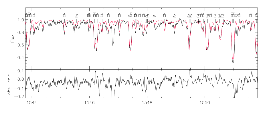
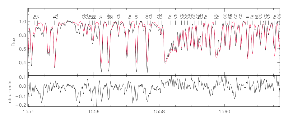
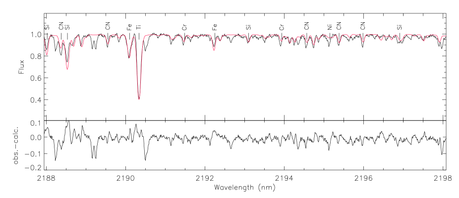
Figure 5: Typical example of a spectral fit achieved in this work, for star J180313.9-295621. The upper, middle, and lower panel show chip 2 and 3 of the H-band setting (order 36), and chip 2 from the K-band setting with order 26, respectively. The upper sub-panel in each panel shows in black the observed spectrum and in red the best-fitting interpolated synthetic spectrum. The lower sub-panel in each panel shows the residuals (observed – calculated flux) of the fit. This star was found to have $T_{\rm eff}=3400$ K, $\log g=+0.05$, $[{\rm Fe}/{\rm H}]=-0.26$, and C/O=0.29.

We may thus assume that the ability to model the spectra of our sample stars is mainly limited by the (in)completeness of available line lists, except for the coolest stars ($T_{\rm eff}\lesssim 3000$ K), for which the hydrostatic models are not realistic and water starts to play an important role. At this low a temperature, the metal lines lose their power to constrain the metallicity and the results for these cool stars are not reliable. Thus, abundances for stars cooler than $T_{\rm eff}=3000$ K are not reported in Table 2.

Most notably, it is not possible to model the spectra of the four LAVs in the Spitzer sample, even though they were observed close to minimum light when their spectra are supposed to be least complex. A model spectrum using only the line list of water by Rothman et al. (2010) was calculated, based on one of the cool models ($T_{\rm eff}=2800$ K) to compare it to observed cool star spectra. Many of the strong lines in the observed spectra have a counterpart in the synthetic water spectrum, suggesting that water is indeed a strong contributor to the spectrum of these stars. This comparison also shows that the match in wavelength between observed spectrum and water line list is good at this high a resolution.

The abundance determination was however successful for the two warmest Plaut stars, even though they are large amplitude variables.

We note that our analysis represents a significant effort. The computation of a single opacity table with one abundance combination takes 19 hours on a fast, modern desktop PC. The construction of the model atmospheres requires significant human interaction because the models do not easily converge at low $\log g$. A more detailed analysis is beyond the resources available to us currently.

3.4 The carbon isotopic ratio and metal abundances

To determine abundances of metals as well as the carbon isotopic ratio, we established for each star a tailored model atmosphere adopting the stellar parameters derived in Sect. 3.1 and assuming the general abundance pattern ([Fe/H], C/O) as found from the H-band spectra (and chip 2 of order 26, where available).

The carbon isotopic ratio was derived from lines of ¹³CO located in chip 1 of grating order 24. An inspection of the optical depth of line cores as a function of gas temperature reveals that the low-J (R19, R22, R24, R26) ¹³CO 2-0 lines are formed relatively far out in the atmosphere where dynamic effects may cause significant deviations of the model atmosphere from the real atmosphere. The analysis was thus based on the high-J 2-0 lines (R76, R78, R80, R81). These lines are also more sensitive to changes in ¹²C/¹³C than the low-excitation lines. Spectra with ¹²C/¹³C ratios of 3.5 (equilibrium value of the carbon isotopic ratio in the CN cycling), 7, 12, 20, 30, 50, and 90 (solar value) were synthesised based on the tailored model atmospheres. The isotopic ratio of the stars cooler than 3000 K, for which no general abundance pattern could be determined, was measured with a generic abundance combination of [Fe/H]=0.0, $[\alpha/{\rm Fe}]=+0.20$, and C/O=0.30. Their isotopic ratios are more uncertain and are marked by a colon in Table 2. Again, an interpolation and fitting routine was employed to determine the value of isotopic ratio that best fits the observed spectrum in the mentioned lines. Figure 6 shows a typical example fit to the ¹³CO 2-0 R76 line of the star J174123.6-282723. Note the good fit also to the ¹²CO 4-2 R64 line at the right hand side of the figure, which gives additional confidence in the C/O ratio that was derived for this star (0.39), though the CO $\Delta\nu=2$ lines in the K-band are generally less sensitive to C/O than the CO $\Delta\nu=3$ lines in the H-band.

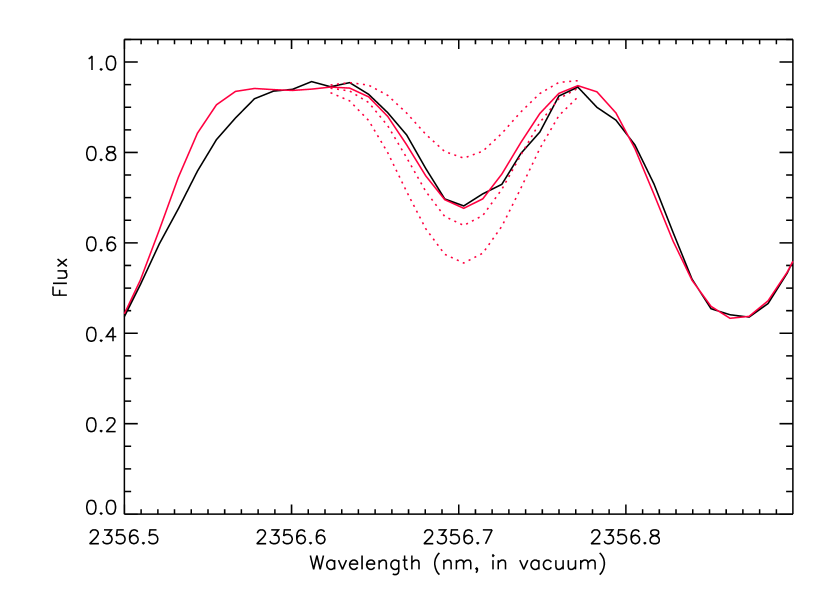
Figure 6: Fit to the ¹³CO 2-0 R76 line of the star J174123.6-282723. The solid red line shows the synthetic spectrum interpolated to the best-fit ¹²C/¹³C=18.2. The dotted lines show the synthetic spectra calculated with ¹²C/¹³C=50, 12, and 3.5 (from top to bottom).

We also aimed at deriving abundances of individual metals using equivalent width (EW) analysis. Weak enough ($\log({\rm EW_{obs}}/\lambda)<-4.5$) but unblended lines of Al, Si, Ti, and Y were found in the spectra in grating orders 26 and 27. Y is a heavy element produced in the slow neutron-capture (s-) process, an increase in its abundance can indicate recent or ongoing 3DUP activity in an AGB star. Astrophysical gf values of the lines were established with the Arcturus spectrum (Hinkle et al., 1995), adopting the abundances for Al, Si, and Ti reported in Ramírez & Allende Prieto (2011), and a scaled solar abundance for Y. Other atomic parameters were taken from the VALD database (Kupka et al., 2000). The resulting line list is reported in Table 3. Synthetic spectra with varying abundances of the individual elements were calculated from the tailored model atmospheres, from which the EWs of the respective lines were measured. The abundance in each star was then calculated by interpolating in the $\log({\rm EW_{synth}}/\lambda)$ vs. $\log\epsilon({\rm X})$ plane to the observed reduced EW ($\log({\rm EW_{obs}}/\lambda)$).

Table 3: Line list used in the determination of the metal abundances. Meaning of the columns: chemical symbol of the element; wavenumber of the transition; oscillator strength gf; excitation energy of the lower level in $10^{4}{\rm cm}^{-1}$.

Element	$\sigma$	gf	$\xi$
	(cm-1)		($10^{4}{\rm cm}^{-1}$)
Al I	4713.8730	3.291e–1	4.13194
Al I	4713.8810	3.291e–1	4.13194
Si I	4779.4609	3.104e+0	5.42569
Ti I	4589.4991	1.256e–1	1.41066
Y I	4702.2860	1.000e–1	1.15337

3.5 Abundance error estimate

To estimate the formal errors on the measured abundances, uncertainties in four quantities were taken into account: temperature, surface gravity, continuum placement, and microturbulence.

An estimate of the temperature uncertainty may be derived from the scatter that most stars exhibit around the general trend of decreasing temperature with increasing luminosity in the HRD (Fig. 3). If the LAVs and the obviously deviating Plaut stars are excluded, the remaining sample stars follow a linear least squares fit in $T_{\rm eff}$ vs. uncorrected luminosity with a standard deviation of 181 K. For the stars with known pulsation period the scatter reduces from 175 K before correction to 119 K after correction. Note that the relation between temperature and luminosity may have an intrinsic scatter and curvature (as indicated by the isochrone in Fig. 3), and that the temperature is not pulsation-cycle averaged. We may thus assume that the uncertainty of the temperature determination is not larger than this scatter. An uncertainty of $\pm 100$ K was adopted.

To estimate the uncertainty on the surface gravity ($\log g$), we adopted the temperature uncertainty, an uncertainty on the luminosity of 10%, and on the pulsation period of 1%. These uncertainties were applied to the formulae given in Sect. 3.1.4. From this, a typical uncertainty of $\Delta\log g=\pm 0.12$ was derived.

The continuum placement was changed by $\pm 1$% and the microturbulence $\xi$ by $\pm 1$ km s^-1. The latter seemed a reasonable uncertainty from the CO lines in the K-band, which are quite sensitive to $\xi$. To determine the abundance uncertainty, the model atmospheres and synthetic spectra were recalculated, varying the parameters one at a time by the given uncertainties, and the spectral fitting was repeated for a few representative stars. The total uncertainty on the abundances was calculated by combining the individual sources of error in quadrature.

The general abundance pattern ([Fe/H], C/O) turned out to be quite robust. The metallicity is most sensitive to temperature and $\xi$, whereas the C/O ratio is most sensitive to changes in $\log g$ and $\xi$ (the CO lines in the H-band are quite sensitive to $\log g$). Changes in [Fe/H] due to temperature uncertainty vary between 0.01 and as much as 0.21 dex, but usually they are $\sim 0.06$ dex. Typical combined uncertainties on [Fe/H] and C/O are 0.10 dex and 0.08, but C/O is more robust at high values ($\pm 0.05$ at C/O=0.50). The C/O ratio was found to change by about 0.1 if $\log g$ is varied by $\pm 0.3$ dex. This means that changing the stellar mass, and hence $\log g$, within any reasonable limits does not significantly change our results and conclusions on the C/O ratio of the stars.

The parameter having the largest impact on the ¹²C/¹³C ratio is the C/O ratio. Changing it by 0.10 can change the isotopic ratio by as much as $\sim 30$%. The errors are correlated: An overestimate (underestimate) of C/O will also lead to an overestimate (underestimate) of ¹²C/¹³C, because with initially stronger (weaker) CO lines it takes less (more) ¹³C to get the same line strength. The surface gravity and continuum placement have some influence on the ¹²C/¹³C ratio, but is limited to $\sim 10$% and $\sim 7$%, respectively. We estimate a combined uncertainty of $\pm\sim 33$% on the ¹²C/¹³C ratio, comparable to literature values.

Typical uncertainties for the elemental abundances are $\pm 0.11$ for [Al/Fe], $\pm 0.25$ for [Si/Fe], $\pm 0.13$ for [Ti/Fe], and $\pm 0.16$ for [Y/Fe].

3.6 Comparison stars

To test our tools for abundance determination, we applied them to a few comparison stars. The goal of this exercise was not to check literature results, but rather to compare abundances derived with our tools to those from other studies and to identify possible systematic differences.

The most important comparison object in studies of cool stars is of course Arcturus. A grid of model atmospheres spanning the same range of [Fe/H] and C/O values as for the science targets was calculated, adopting the stellar parameters determined by Ryde et al. (2010), which are: $T_{\rm eff}=4280$ K, $\log g=1.7$, and $\xi_{\rm micro}=1.7$ km s^-1. Synthetic spectra were generated and fitted to the observed, high-resolution spectrum provided by Hinkle et al. (1995) in the same spectral range in which the science targets were observed with CRIRES. The fitting routine converged at a metallicity of $[{\rm Fe}/{\rm H}]=-0.50$, which agrees very well with the value of $[{\rm Fe}/{\rm H}]=-0.53\pm 0.05$ derived by Ryde et al. (2010). Our C/O ratio of 0.32 is somewhat higher than 0.24 as found by these authors, whereas Rich & Origlia (2005) determined C/O=0.28 in Arcturus. Since Arcturus is a K-type giant whose atmospheric structure is less influenced by molecular opacity than that of M-type giants, we also performed the 3D fit introduced in Sect. 3.3. With this approach the following abundance pattern for Arcturus was found: $[{\rm Fe}/{\rm H}]=-0.51$, C/O=0.37, and $[\alpha/{\rm Fe}]=+0.31$. The $\alpha$-abundance ratio is in excellent agreement with the value of +0.33 found by Ryde et al. (2010) from an average of the abundance of O, Si, S, and Ti. We also modelled the observed CRIRES spectra of the comparison stars BMB 78, BMB 289 (both located in the Galactic bulge), and BD$-$012971 (a solar neighbourhood star). The stellar parameters of these stars were not determined as for the science targets, rather the parameters provided by Cunha & Smith (2006) and Rich & Origlia (2005), respectively, were adopted (see Table 1). The results of our abundance determination as well as the literature values are summarised in Table 4.

Table 4: Comparison of abundances with literature results.

Name	[Fe/H]	[Fe/H]	C/O	C/O	12C/13C	12C/13C	Ref.
	this work	lit.	this work	lit.	this work	lit.
BMB 78	$-0.47$	$-0.03$	0.46	0.20	9.9	…	CS06
BMB 289	$-0.05$	$-0.05$	0.57	0.28	4.0:	…	CS06
BMB 289	$-0.21$	$-0.15$	0.67	0.12	4.6:	$5.0\pm 1.2$	RO05
BD$-$012971	$-0.68$	$-0.24$	0.30	0.15	9.5	$7.9\pm 1.8$	RO05
BD$-$012971	$-0.68$	$-0.78$	0.30	…	9.5	…	RS15

The differences to the literature values vary from star to star. Our [Fe/H] is lower than the literature [Fe/H] value by more than 0.4 dex for BMB 78 and BD$-$012971, whereas for BMB 289 the agreement in the metallicity is excellent (the fit to the observed spectrum of that star is somewhat better with the parameters of Rich & Origlia, 2005). However, the metallicity of BD$-$012971 was recently also determined independently by Ryde & Schultheis (2015) using different data to be $[{\rm Fe}/{\rm H}]=-0.78$, in good agreement with our result ($[{\rm Fe}/{\rm H}]=-0.68$).

The C/O ratio found in our modelling is higher than the literature value by large factors in some cases. To identify the reason for this difference, the original spectra of the comparison stars obtained by Rich & Origlia (2005) and Cunha & Smith (2006) were kindly made available to us by these authors. A comparison showed that the spectra of BMB 78 and BD$-$012971 are indeed very similar to ours, i.e. the difference in the abundances can not be attributed to the different observational material. Some variation can be seen for the spectra of BMB 289. This star is identified by Soszyński et al. (2013) to be a semi-regular variable with a primary pulsation period of 162.53 d and an I-band amplitude of 0$\aas@@fstack{m}$132. Most likely, the difference seen in the spectra is due to dynamic effects in the atmosphere of that star. The fit to the spectrum of BMB 289 is of lower quality than for the other stars. Also, because of its late spectral type (M9, Blanco et al., 1984), this star could be considerably cooler than assumed in the literature. For these reasons, BMB 289 appears to be not a good comparison star and we put less weight on it.

The C/O ratios reported by Rich & Origlia (2005) are very low. Using the abundance pattern given in the literature, our models do not give a proper fit of the observed spectra. Note that $T_{\rm eff}$ and $\log g$ as given in the literature were adopted. The reason for the differences found in the C/O ratios must lie in the different analysis methods. Because of the insensitivity of the OH lines available here to the O abundance in M-type giants (Sect. 3.3), we assumed a priori a trend of the O abundance with metallicity that was derived from hotter stars. This trend might not be applicable to our sample. However, we believe that most of the difference in the results stems from inconsistencies in the O abundance used for model construction and for spectral synthesis, which may produce different C/O ratios. We should add that the measured C/O ratios in our sample are expected to be reliable at least in a relative sense, so that we are able to draw conclusions on the occurrence of internal C enrichment by 3DUP.

Table 4 also collects the ¹²C/¹³C ratios reported in the literature (Rich & Origlia, 2005) and measured here. The ratio is quite uncertain for BMB 289, but for BD$-$012971 the agreement is very good.

In conclusion, the agreement with literature results on the individual star level is mixed. The excellent agreement that was found for the well-studied star Arcturus however gives confidence that the abundance patterns that we derived for our science targets are reliable. As shown in Sect. 4.2, the good agreement in mean metallicity on the level of late-type star samples in the inner bulge regions gives us further confidence in our results.

4 Results and discussion

In most of the following subsections, the Plaut stars need to be discussed separately from the Spitzer stars because they stand out from the sample in terms of location in the bulge, but also in metallicity and C/O ratio. Comparisons with other bulge samples are based only on the Spitzer sample because of closer spatial overlap. We ask the reader to pay attention to which subsample is discussed in which place.

4.1 Current masses

The current masses may tell us something about the age of the sample stars and the star formation history in the Galactic bulge. Due to stellar mass loss, the initial masses must have been higher than the current masses. Some of the masses listed in Table 1 are significantly larger than $1.0M_{\sun}$, implying ages considerably lower than 10 Gyrs. This is in agreement with what was found previously from studies of AGB stars in the bulge (van Loon et al., 2003; Groenewegen & Blommaert, 2005; Uttenthaler et al., 2007): luminosities, pulsation periods, and dredge-up behaviour suggest that there are stars of masses $1.5-2.0M_{\sun}$ and intermediate age ($\lesssim 5$ Gyrs) present in the bulge. Although not obvious in purely photometric studies of the turn-off (Zoccali et al., 2003; Clarkson et al., 2008, 2011), recent investigations of microlensed dwarf and sub-giant stars with known metallicities by Bensby et al. (2013) indicate that a younger population is probably present in the bulge. The masses derived for our sample stars are in line with those results. An extended star formation history is required to explain the more massive AGB stars in the bulge.

The four LAVs among the Spitzer sample seem to form a distinct group. They have the following independent properties that distinguish them from the other stars: their spectra, with very strong TiO and VO bands, make them the coolest stars observed; their luminosities, if corrected for the depth scatter, would be the highest of the stars in the sample; they have the longest observed pulsation periods, from 392 to 472 days; and they have both the lowest and highest radial velocities of any of the stars observed, suggesting that their velocity dispersion is higher than that of the other stars. The probability to find the extreme RV values among any sub-sample of four stars within our Spitzer sample of 37 stars is 0.9%. The upper panel of Fig. 7 shows the distribution of the Spitzer sample stars in the RV vs. period diagram. The lower panel of that figure shows a band strength index (pseudo-continuum: $911-921$ nm, band: $923-938$ nm) as a function of period. This band strength index shows a very strong linear correlation with the determined temperature. The four LAVs are plotted as red symbols. The four LAVs not only have the highest and lowest radial velocity, they also have the strongest molecular bands, indicating that they form a distinct group among the Spitzer sample.

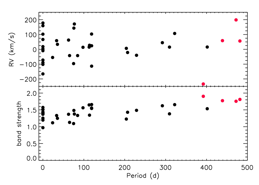
Figure 7: Radial velocity and band strength index as a function of pulsation period of the Spitzer sample stars. The LAVs are shown as red symbols. The extreme velocities as well as the highest band strengths are found among the stars with the longest periods. Stars for which no period is known are set to $P=0$.

The high luminosities of these stars are consistent with their high derived masses in that high-mass stars evolve further up the AGB before they eject all their envelopes. The very low temperatures, especially if the stars really are massive, suggest that these stars are of high metallicity since the giant branch becomes cooler with increasing metallicity, but hotter with increasing mass. Unfortunately, their near-IR spectra are too complex to derive any abundances from them.

Wood & Bessell (1983) observed a similar group of long period variables in the bulge and they also deduced masses of $3-5M_{\sun}$. They concluded that these objects had metallicities about $2.5Z_{\sun}$ and suggested that they could be young metal-rich stars ejected from star-forming regions in the Galactic plane near the centre of the Galaxy. Star clusters recently formed near the Galactic centre are now well known (e.g. Wang et al., 2006). The $3-5M_{\sun}$ stars could also be ejected from the central star cluster where young stars are known to exist (Genzel et al., 2010). The high RV dispersion obtained for the present sample of four cool, high-luminosity, long-period variables lends support to this suggestion.

4.2 Metallicity

The metallicity distribution function (MDF) of the sample stars is shown in the middle panel of Fig. 8. The Plaut stars are included in this diagram. The MDF is symmetric and shows a clear peak between $[{\rm M}/{\rm H}]=-0.10$ and $-0.20$.

Figure 8: Top panel: Histogram of the C/O ratios. Middle panel: Histogram of the metallicity of all sample stars with reliable metallicity determination. Bottom panel: C/O ratio as a function of metallicity. The Plaut stars are shown as red symbols, also two typical error bars are shown.

The median metallicity of the Spitzer sample is $[{\rm M}/{\rm H}]=-0.15$, the mean is $\left<[{\rm M}/{\rm H}]\right>=-0.14\pm 0.03$, with a standard deviation of $0.15\pm 0.02$ dex. Only few stars have super-solar metallicity. The Spitzer sample appears to be very homogeneous. The result for the Spitzer sample may be compared to some results from the literature: Rich & Origlia (2005) find $\left<[{\rm Fe}/{\rm H}]\right>=-0.19\pm 0.02$ from the analysis of high-resolution ($R=25\,000$) H-band spectra of 14 M-type giants in Baade’s Window at $(l,b)=(+1\degr,-3.9\degr)$, in excellent agreement with our result. The $1\sigma$ dispersion in their sample is $0.080\pm 0.015$ dex, somewhat narrower than in ours. Cunha & Smith (2006) analysed high-resolution ($R=50\,000$) H- and K-band spectra of seven bulge K- and M-type giants and derive $\left<[{\rm Fe}/{\rm H}]\right>=-0.15$. Despite some disagreement with those works on individual objects (Sect. 3.6), the mean metallicities of the samples agree. Rich et al. (2007) observed 17 M giants in a field $1\degr$ south of the Galactic centre and measure $\left<[{\rm Fe}/{\rm H}]\right>=-0.22\pm 0.03$ with a $1\sigma$ dispersion of $0.140\pm 0.024$ dex. Finally, Rich et al. (2012) observed a total of 30 M giants in two fields $1.75\degr$ and $2.65\degr$ south of the Galactic centre and find in these fields $\left<[{\rm Fe}/{\rm H}]\right>=-0.16\pm 0.03$ and $\sigma=0.12\pm 0.02$, and $\left<[{\rm Fe}/{\rm H}]\right>=-0.21\pm 0.02$ and $\sigma=0.09\pm 0.016$, respectively. All these results for (non-variable) K- and M-type giants agree very nicely with our result for the Spitzer sample.

A lack of metal-rich stars among M-type giants in the bulge was noted in previous works (e.g. Uttenthaler et al., 2012; Rich et al., 2012, and references therein). This is surprising because only relatively metal-rich stars would be expected to become cool enough to evolve to M-type giants. Figure 9 shows a comparison between MDFs of in total 61 bulge M-type giants (Rich & Origlia, 2005; Rich et al., 2007, 2012) and AGB stars (27 stars, this work), and the MDF of bulge dwarf and subgiant stars (58 stars, Bensby et al., 2013). While the MDFs of M-giants and AGB stars are quite narrow and peak between $[{\rm Fe}/{\rm H}]=-0.3$ and $-0.1$, the MDF of dwarfs is much broader with less clear peaks. The last also contains more metal-rich stars than do the giant samples. A two-sided Kolmogorov-Smirnov test reveals that the probability that our Spitzer and the dwarf star sample are drawn from the same underlying population is only 0.01. For the 61 M giants and the dwarf sample, the mutual probability is even less than $10^{-5}$.

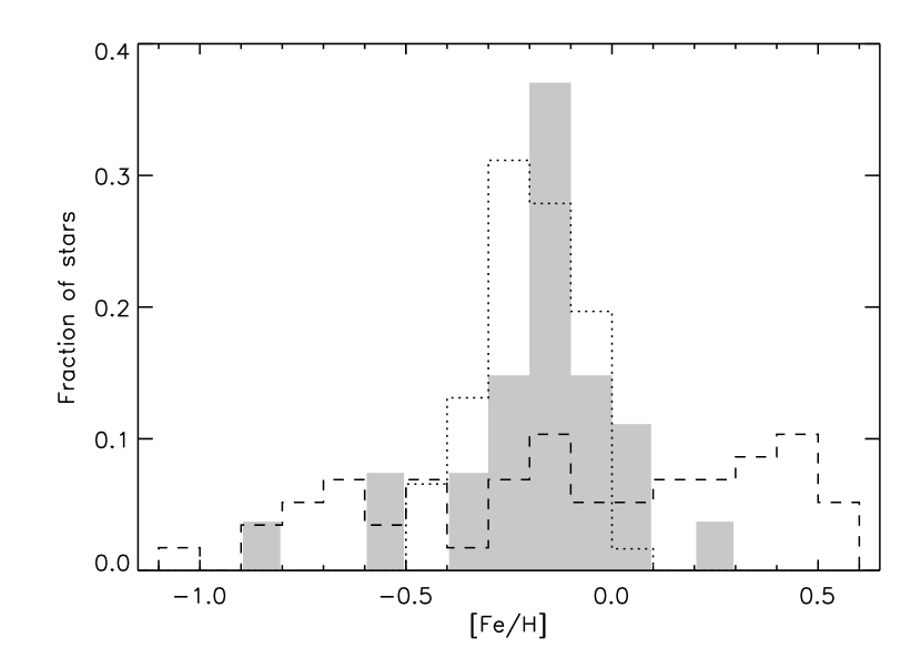
Figure 9: Comparison of MDFs: this work (shaded histogram); combined MDF from Rich & Origlia (2005), Rich et al. (2007), and Rich et al. (2012, dotted line); and Bensby et al. (2013, dashed line).

It has been suggested that very high mass-loss rates at high metallicities could remove those stars from the canonical paths of stellar evolution (Cohen et al., 2008; Castellani & Castellani, 1993), hence they do not reach the coolest and most advanced phases. The low number of super-solar metallicity stars in our sample is in agreement with this conjecture.

On the other hand, Buell (2013) finds that bulge PNe descend mostly from super-solar metallicity stars. This result may be biased towards high-metallicity objects because only PNe with relatively high surface brightness can be studied at the distance of the bulge. Furthermore, metal-rich stars may be more likely to form PNe than metal-poor ones, e.g. due to enhanced mass loss and/or a higher binary fraction.

The two Plaut stars for which a metallicity could be determined have a lower metallicity than the remaining sample (one Spitzer sample star has the same metallicity as one of the Plaut stars). Though not a strong confirmation, this finding is consistent with the conclusion of Uttenthaler et al. (2012) that AGB stars in the outer bulge ($b\approx-10\degr$) descend mainly from the metal-poor bulge population, not from the metal-rich one. This conclusion was however solely based on the kinematical properties (radial velocity dispersion) of AGB stars and of the metal-poor and metal-rich population of RGB stars in a field centred on $(l,b)=(0\degr,-10\degr)$, not on actual metallicity determinations. Uttenthaler et al. (2012) found the metal-poor population in that field to have a mean metallicity $[{\rm M}/{\rm H}]=-0.57\pm 0.03$ with a dispersion of $0.28\pm 0.03$ dex. The two Plaut stars analysed here fall well into this distribution, which suggests that they actually descend from this metal-poor bulge population. Note however, that non-negligible biases could influence this finding: Of the 671 long-period and semi-regular variables found by Plaut (1971) in the Palomar-Groningen field no. 3, 27 were selected for optical spectroscopy by Uttenthaler et al. (2007), of which only eight have been observed with CRIRES and analysed here, four of them being Tc-rich.

A negative metallicity gradient has previously been found along the minor axis of the Galactic bulge (Zoccali et al., 2008). Our complete sample is in agreement with such a gradient because the metal-poor Plaut stars are far from the plane. Even when only the Spitzer sample is considered, we find a slight negative metallicity gradient, but this is not very significant.

4.3 C/O and carbon isotopic ratios – Which AGB stars undergo 3DUP?

All sample stars are oxygen-rich, i.e. there is no carbon star in the sample. Also among those sample stars whose abundances could not be measured, none has an enhanced strength of the CO band head, except for the Plaut stars with Tc. The distribution of C/O ratios in the sample is shown in the upper panel of Fig. 8. Our sample shows an even distribution of C/O ratios between 0.22 and 0.51, again except for the Plaut stars, which have a considerably higher C/O ratio. This was expected because these two stars were found to show lines of Tc, an indicator of recent or ongoing 3DUP. A comparison between the spectra of the Plaut stars with those of similar stars from the Spitzer sample shows that the former indeed have much more prominent CO and CN lines. Hence, the two Plaut stars are a good benchmark of which C/O ratio we may expect to find in stars that underwent 3DUP and to check if any of the Spitzer sample stars underwent 3DUP.

The mixed chemistry observed in many Galactic bulge PNe (Guzman-Ramirez et al., 2011) may be understood if those objects descend from stars such as the Tc-rich Plaut stars. They have an enhanced C/O ratio ($\gtrsim 0.7$), which would ease the formation of PAHs in their outflows once they become post-AGB objects or PNe. Our finding of a relatively high C/O ratio in two of the Plaut stars (${\rm C}/{\rm O}\sim 0.7$) does not exclude the existence of an UV-irradiated torus around the central stars of Galactic bulge PNe suggested by Guzman-Ramirez et al. (2011). Nevertheless, our observations suggest that the assumption of low C/O ratios in PNe precursors towards the Galactic bulge is not easily justified.

The solar C/O ratio in the compilation of Caffau et al. (2008) used here is 0.55, hence all Spitzer sample stars have an at least slightly sub-solar C/O ratio. The mean C/O ratio of the Spitzer stars is 0.38, with standard deviation of 0.10. Careful measurements of the C/O ratio in K-type bulge giants find somewhat lower ratios than this. For example, Meléndez et al. (2008) find a mean of 0.24 in a sample of 19 K-type giants, and Ryde et al. (2010) find a mean of 0.26 among 11 stars. Although the Spitzer sample has a somewhat higher mean C/O ratio than these K giant samples, we do not think that the sample contains stars that underwent 3DUP. Rather, there could be systematic effects between the analysis of the AGB stars here and the hotter K-type giants.

Stars that have undergone 3DUP events may be revealed by a plot of the carbon isotopic ratio vs. C/O, since both these ratios are expected to be enhanced. Such a diagram is presented in Fig. 10. Included in that diagram are solar neighbourhood red giants from Smith & Lambert (1990): Filled blue triangles represent giants of type M or MS with Tc, open blue triangles are M-type giants without Tc. Tc-poor MS/S-type stars are not included here because they are thought to be the product of binary mass transfer. To guide the eye, the evolution of AGB atmospheric abundance patterns by adding ¹²C to them is indicated by the two dashed lines in Fig. 10. This is a rather simplistic view because it ignores possible effects of deep mixing on the AGB (Busso et al., 2010). The operation of deep mixing can considerably mask the 3DUP evidence because ¹²C will be consumed to from ¹⁴N. Indeed, not all of the Tc-rich stars in Fig. 10 have an enhanced C/O or ¹²C/¹³C ratio, and there are Tc-poor stars that have a higher C/O ratio than some of the Tc-rich stars have. The disc giants discussed in the Appendix may give a further indication of typical abundance ratios found in pre-3DUP giants. However, there are a few disc stars in Fig. 10 that have obviously added a considerable amount of ¹²C to their atmospheres. The only star from our sample that is displaced from the rest is Plaut 3-942 (filled red diamond symbol), a star with known Tc content. Its ¹²C/¹³C ratio is uncertain, but seems to be higher than that of most of the other sample stars. Unfortunately, it was not possible to determine the ¹²C/¹³C ratio in Plaut 3-626.

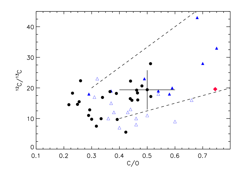
Figure 10: Carbon isotopic ratio vs. C/O. Filled black circles represent stars from this work, while filled blue triangles are Tc-rich MS- or S-type, open blue triangles Tc-poor M-type giants from Smith & Lambert (1990). The filled red diamond symbol is the Tc-rich star Plaut 3-942. The two dashed lines indicate the evolution of atmospheres with (C/O,¹²C/¹³C)=(0.30,20) and (0.40,10) by adding ¹²C to them. A typical error bar is shown for one star (J174917.0-293502).

The Spitzer sample star with the highest ratios is J180308.7-295220 at C/O=0.51 and ¹²C/¹³C=28. Note, however, that the errors in these quantities are correlated, an overestimate in C/O also leads to an overestimate in ¹²C/¹³C, see Sect. 3.5. This star does not show an enhanced Y abundance in its atmosphere (Table 2). Also, none of the cool stars for which no metallicity or C/O ratio could be determined has a significantly enhanced ¹²C/¹³C. Therefore, we believe that none of the Spitzer sample stars has undergone a 3DUP event yet (although they may have undergone He-shell flashes without 3DUP). The same conclusion is reached from the location of the sample stars in a dust mass-loss rate ($K-[22]$) vs. pulsation period diagram, which allows to distinguish between Miras with and without Tc (Uttenthaler, 2013). This also implies that C/O and ¹²C/¹³C are not useful as “evolutionary clock” for the Spitzer sample, as initially anticipated for the observations.

With the sample of stars for which we have information on the current mass and the metallicity, we may put constraints on AGB evolutionary models that make predictions concerning the occurrence of 3DUP and the formation of carbon stars. It is difficult to obtain the mass and metallicity of an AGB star, because it requires a star to pulsate in order to derive its mass, but dynamic effects caused by the pulsations hamper the determination of the metallicity. Nevertheless, in Fig. 11 the stars are plotted in the mass – metallicity plane, along with predictions from model tracks calculated with the COLIBRI code (Marigo et al., 2013). The maximum C/O ratio reached by the model stars is colour-coded in that diagram: stars in the light coloured area in that plane turn into carbon stars at least for some time on the AGB, the darker the colour the lower the maximum C/O ratio. The minimum initial mass required for a star to experience 3DUP or to become a carbon star increases with increasing metallicity because the mixing is less efficient at higher metallicity. At solar metallicity, the models of Marigo et al. (2013) predict that a minimum initial mass of 1.90 $M_{\sun}$ is required to form a carbon star, and the interpulse luminosity these stars is predicted to be in the range $2000-6000L_{\sun}$. Our sample stars (white symbols) have sub-solar metallicity, but their current masses would be too small to undergo significant 3DUP.

Figure 11: Formation of carbon stars and 3DUP behaviour in the initial mass vs. metallicity plane of models from Marigo et al. (2013). Light coloured areas indicate a combination of mass and metallicity where the model star becomes carbon-rich for at least a short while on the AGB. The darker the colour, the lower the maximum C/O ratio reached by the model star. The white symbols are sample stars for which a current pulsation mass and a metallicity was determined: circles are for Spitzer sample stars, diamonds for Plaut stars.

The two Plaut stars, which are at moderately low metallicity and clearly experienced 3DUP, are also in a region of the diagram where the models do not predict 3DUP to happen, clearly in contradiction with observations. In principle, 3DUP should be eased in these stars because of their lower metallicity. Nevertheless, at the metallicity of the Plaut stars, the models predict that a higher initial mass is required for 3DUP to occur than the Plaut stars have. The initial masses of the stars must have been higher than the current masses, but it is not expected that they have lost a significant amount of their mass. The largest mass loss occurs during the super-wind phase on the AGB, which our stars have not yet entered, except maybe the ones with the highest mass-loss rates. If the determined current masses are reliable and if they have not been lowered much from the initial value by mass loss, then the evolutionary models would predict 3DUP to occur at too high initial masses at these moderately low metallicities.

A number of sample stars with a high current mass but without measured metallicity might fall in the range where carbon star formation is predicted by the models. Since all of these stars are oxygen-rich, they are problematic for the evolutionary models, unless they have a considerably higher metallicity than the other sample stars. This may be the case for the LAVs in the Spitzer subsample, see Sect. 4.1. We caution that there is also the possibility that the linear pulsation models are not adequate to derive the current masses of some of the stars, or that the input stellar parameters for the mass determination (e.g. temperature) are in error.

The lower panel of Fig. 8 shows the C/O ratio as a function of metallicity. It is clear that the Spitzer sample stars are quite homogeneous in their overall composition, with metallicities mostly sub-solar and all C/O ratios below the solar value. The Plaut stars (red symbols) are clearly offset from this group. Our sample does however not allow to infer the evolution of the C/O ratio with metallicity in the bulge region. For models and observations of the C/O evolution, we refer to Cescutti et al. (2009).

4.4 Metal abundances

Only the Spitzer sample stars were observed in the additional K-band setting; the individual metal abundances derived from them are discussed here. The results of these measurements are presented in Fig. 12. The scatter in the abundances may be fully explained by measurement uncertainty (see the error bars on the left hand side of the panels). The abundances are compared primarily to measurements in similar regions of the bulge as the location of the Spitzer sample stars (Bensby et al., 2013; Alves-Brito et al., 2010; Gonzalez et al., 2011). Only for Al measurements from the outer bulge (Plaut’s field, $b\approx-8\degr$) from Johnson et al. (2012) are included. The Spitzer sample is too small and spans too small a range in metallicity to probe for any trends of the elements with metallicity. However, the abundances are suited to check if the AGB stars in the present sample descend from the same populations that can be found among less evolved bulge stars. A look at Fig. 12 can answer this question with “yes”: The relative abundances of Al, Si, Ti, and Y agree well with the range of abundances that are seen in other bulge stars at these metallicities. The fact that Y, one of the light s-process elements, is not significantly enhanced also argues against 3DUP being active in the Spitzer sample stars for which the Y abundance could be derived. Also, no correlation between [Y/Fe] and C/O is found in our data. C and Y are thus probably not produced in situ and the abundances likely reflect the primordial values.

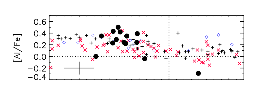
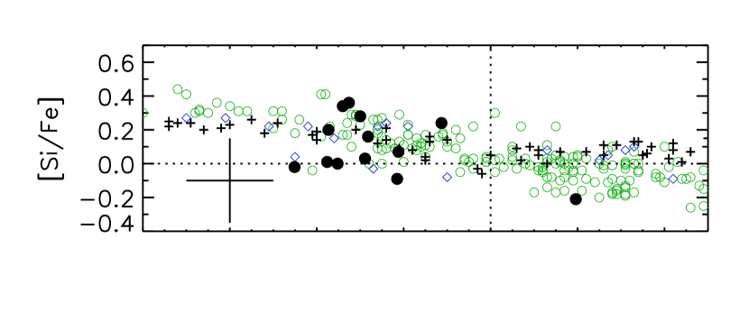
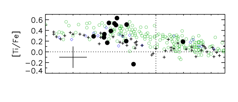
Figure 12: Abundances of [Al/Fe], [Si/Fe], [Ti/Fe], and [Y/Fe] as a function of [Fe/H] (from top to bottom) in samples of Galactic bulge stars. Filled black circles are data points from this work, black plus symbols are dwarf and subgiant stars from Bensby et al. (2013), blue open diamonds are from Baade’s field from Alves-Brito et al. (2010), green open circles from Gonzalez et al. (2011, only Baade’s field), and red crosses are from Plaut’s field in the outer bulge from Johnson et al. (2012). The big symbols on the left hand side of each panel show typical error bars.

4.5 Radial velocities

Here only the heliocentric radial velocities of the 37 Spitzer sample stars (column 2 in Table 2) are discussed. For the radial velocity dispersion of AGB stars in the outer bulge, see Uttenthaler et al. (2012, Section 4.7.3).

The radial velocities of the Spitzer stars have a mean of $\left<{\rm RV}\right>=16.1\pm 15.8$ km s^-1 and a dispersion of $\sigma_{\rm RV}=95.8\pm 11.3$ km s^-1. However, it appears that the RV dispersion depends on the latitude of the fields (Fig. 13): while in the field at $b\sim-3.8\degr$ the dispersion of the 17 stars is only $65.9\pm 11.6$ km s^-1, the fields at $b\sim\pm 1\degr$ (15 stars) have a combined dispersion of $115.0\pm 21.7$ km s^-1. It has been shown that the metal-rich stellar population of the Galactic bulge has a radial velocity dispersion that significantly increases when approaching the plane, whereas the metal-poor population has a constant $\sigma_{\rm RV}$ of 90 – 100 km s^-1 throughout the bulge (Babusiaux et al., 2010; Uttenthaler et al., 2012; Babusiaux et al., 2014). This increasing radial velocity dispersion is a result of the action of the Galactic bar. We thus suggest that the Spitzer sample also follows a bar-like kinematic pattern, and that it belongs to the metal-rich population. The metallicities measured in the present paper are in agreement with this picture. Note that Mira stars in the bulge are actually found to trace a tilted bar (Groenewegen & Blommaert, 2005). As shown above that the Plaut stars are more metal-poor. The radial velocity dispersion of AGB stars in the outer bulge suggests that they descend from the metal-poor, spheroidal component of the bulge.

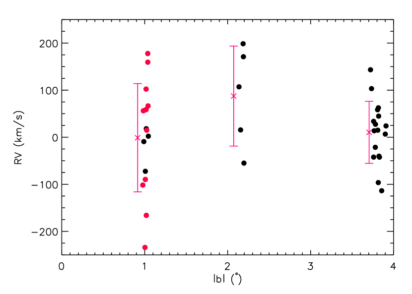
Figure 13: Radial velocity vs. absolute value of Galactic latitude for the Spitzer sample stars. Red symbols represent stars located north of the Galactic plane, at positive latitude. The large symbols next to the three latitude groups show the mean and standard deviation of the radial velocity of the respective group.

5 Conclusions

We present an analysis of high-resolution near-IR spectra of a sample of Galactic bulge AGB stars. The sample consists of a larger sub-sample from the inner and intermediate bulge (Spitzer sample) and a smaller sample from the outer bulge (Plaut stars). Using state-of-the-art hydrostatic model atmospheres for cool stars and the best available atomic and molecular line lists for the observed wavelength range, we are able to successfully model the spectra of stars down to $T_{\rm eff}\approx 3100$ K. General metallicities [Fe/H], the carbon-to-oxygen ratio C/O, carbon isotopic ratio ¹²C/¹³C, the abundance of Si, Al, Ti, and Y, and heliocentric radial velocities are determined. The abundance analysis relies on the assumption of an $[\alpha/{\rm Fe}]$ trend with [Fe/H] because of the low sensitivity of OH lines to the O-abundance in cool, M-type giants. We caution that calculation of both the model atmosphere and the spectral synthesis with consistent abundances is required in such cool stars for a reliable modelling. Current stellar masses are also derived from linear pulsation models.

This paper touches on the problem of the apparent lack of intrinsic carbon stars in the Galactic bulge. All sample stars are oxygen-rich, there is no carbon star among them. The C/O and carbon isotopic ratios measured in the sample stars suggest that the Spitzer sample stars did not undergo the third dredge-up. They appear to have a composition typical for post-first dredge-up red giants. Furthermore, no increased CO band head strength was found among the stars for which we could not measure the overall composition, excluding the known technetium-rich stars. Note, however, that the effect of 3DUP on the carbon abundance may be considerably masked by the operation of deep mixing on the AGB. The conclusion of a lack of 3DUP in these stars is supported by the fact that Y is not enhanced in the stars with observations of a line of that s-element, and the position of the Spitzer stars in a dust mass-loss rate vs. period diagram (Uttenthaler, 2013). On the other hand, two of the Plaut stars have a clearly enhanced C/O ratio, as expected from the fact that Tc lines have been found earlier in their optical spectra.

However, detailed AGB evolutionary models, e.g. Marigo et al. (2013), are in conflict with our measurements of metallicities, masses, and 3DUP occurrence in the sample stars. Those models predict no 3DUP for stars with initial masses as low as the current masses of some of the Tc-rich Plaut stars, but do predict 3DUP and carbon star formation for the more massive stars in our sample. Though it is impossible to determine the metallicity and C/O ratio for the coolest and putatively most massive stars in the sample, it is clear that they are not carbon-rich. Assuming a similar metallicity distribution as the other Spitzer stars, one would expect from the models that they evolve into carbon stars. The reason for this could be that the masses estimated with our linear pulsation models are not accurate enough because of uncertainties on the input parameters and/or invalid assumptions for the models. We suggest that 3DUP is found in the Plaut stars but not in the Spitzer stars because of their lower metallicity, see below. On the other hand, the C-star lifetime is very short at high metallicity, and also a high He abundance could prevent 3DUP and C-star formation (Karakas, 2014).

It has been suggested that a high oxygen abundance could prevent the formation of carbon stars in the Galactic bulge (Feast, 2007). However, the current consensus is that the O-abundance trend in bulge stars is very similar to that of local thick disc stars (Meléndez et al., 2008; Ryde et al., 2010; Bensby et al., 2013). We suggest that at the slightly subsolar metallicity of the Spitzer stars, carbon star formation is suppressed because 3DUP is suppressed altogether, either because of the high metallicity or possibly because of a high He abundance. Hence, an enhanced oxygen abundance is not required to explain the lack of carbon stars in the Galactic bulge. 3DUP does occur at the lower metallicity of the Plaut stars in the outer bulge, but there may not be sufficient 3DUP events to turn them into C-rich stars, and/or because of the action of deep mixing. From the masses that we derive for these stars one might expect C-star formation, but note the uncertainties in the mass determinations.

The Spitzer sample stars have on average slightly sub-solar metallicity but there are few that have super-solar metallicity. This is in agreement with the results of previous observations of cool giant samples in the Galactic bulge, though the comparison on the level of individual stars is more uncertain. The lack of super-solar metallicity stars could be caused by metallicity-dependent stellar winds (Cohen et al., 2008).

The Plaut stars are found to be more metal-poor, in agreement with earlier suggestions by Uttenthaler et al. (2012) that were based on kinematical arguments. Thus, we suggest that the AGB stars in the outer Galactic bulge mainly descend from the metal-poor bulge population ($[{\rm Fe}/{\rm H}]\sim-0.6$), not from the metal-rich one ($[{\rm Fe}/{\rm H}]\sim+0.3$), although about 30% of the RGB stars in a field at $(l,b)=(0\degr,-10\degr)$ belong to the metal-rich bulge population (Uttenthaler et al., 2012). The metallicity inferred for Galactic bulge PNe (Buell, 2013) is higher than what we find among AGB stars. It could be that metal-rich stars are more likely to form PNe, which would be in agreement with the call for metallicity-dependent stellar winds.

The abundances of Al, Si, Ti, and Y measured for some of the Spitzer sample stars suggest that they descend from the bulk of the population in their bulge region. The radial velocity dispersion of the Spitzer stars suggests that they follow a bar-like kinematic pattern, characteristic for the metal-rich bulge population. The Plaut stars, on the other hand, seem to belong to the metal-poor, spheroidal bulge component.

Finally, the masses of the sample stars suggest that the Galactic bulge is not exclusively old, a younger and more massive population ($\sim 1.3M_{\sun}$) seems to be present. This would be in agreement with age estimates of metal-rich dwarf stars in the Galactic bulge (Bensby et al., 2013).

Appendix A Abundances in five field red giants

Observations of five red giant stars in the field have been obtained in the same CRIRES run. These spectra were also analysed and the results are reported here for the sake of completeness.

The determination of the effective surface temperature and gravity of the field stars relied purely on literature values and near-IR photometry. Temperatures of the stars are given by Wright et al. (2003), which are based on spectral type determinations. As a second estimate, we applied the $T_{\rm eff}-(J-K)_{0}$ calibration of Lebzelter et al. (2012) to the $(J-K)_{0}$ colour that was derived from 2MASS photometry (Skrutskie et al., 2006) and the interstellar reddening map of Schlegel et al. (1998). A compromise value between these two estimates was adopted for the model atmospheres. The surface gravity $\log g$ was estimated also with the $\log g-(J-K)_{0}$ calibration of Lebzelter et al. (2012). The stellar parameters of the field giants are summarised in Table 5.

Table 5: Stellar parameters of the field red giants. Meaning of the columns: object name; range of spectral types found in VizieR; J, H, and K magnitudes from 2MASS; interstellar extinction in the V-band from Schlegel et al. (1998); de-reddened $J-K$ colour; effective temperature derived from the $T_{\rm eff}-(J-K)_{0}$ calibration of Lebzelter et al. (2012, L12); effective temperature listed in Wright et al. (2003, W03); adopted effective temperature; adopted $\log g$ of the model atmosphere, estimated with the $\log g-(J-K)_{0}$ calibration of Lebzelter et al. (2012).

Object name	Sp. type	$J$	$H$	$K$	$A_{\rm V}$	$(J-K)_{0}$	$T_{\rm eff}$	$T_{\rm eff}$	$T_{\rm eff}$	$\log g$
		(mag)	(mag)	(mag)	(mag)		(K, L12)	(K, W03)	(K, adopted)	(cgs)
HD136546	K5 III	4.445	3.515	3.313	0.730	1.021	3785	3950	3900	1.20
HD140672	K5-M1 III	4.207	3.251	3.021	0.947	1.042	3740	3720	3750	1.10
HD141189	M0-2 III	4.542	3.551	3.252	0.407	1.228	3295	3620	3400	0.38
HD141311	K5-M1 III	4.849	3.862	3.701	0.776	1.030	3766	3720	3750	1.10
HD141938	M0-2 III	4.314	3.367	3.133	0.574	1.094	3624	3720	3650	0.90

The CRIRES spectra of the field stars, which are of high quality, were analysed in the same way as the bulge AGB stars in the main part of the paper, except that for the $\alpha$-abundance a more disk-like relation was adopted, with $[\alpha/{\rm Fe}]=+0.4$ up to $[{\rm Fe}/{\rm H}]=-1.0$, followed by a decline of 0.4 dex/dex for higher metallicities. The results of the analysis are summarised in Table 6. All five stars have close to solar metallicity, and slightly sub-solar C/O ratios (on the scale of Caffau et al., 2008).

Table 6: Radial velocities and abundances measured for the field red giants. Meaning of the columns: object name; heliocentric radial velocity; metallicity; C/O ratio; carbon isotopic ratio, and relative abundances of Al, Si, Ti, and Y.

Object name	RVhelio	[Fe/H]	C/O	12C/13C	[Al/Fe]	[Si/Fe]	[Ti/Fe]	[Y/Fe]
	(km s-1)
HD136546	$-9.7$	$+0.05$	0.38	15.4	$+0.11$	$+0.05$	$+0.04$	$-0.18$
HD140672	$-27.3$	$+0.04$	0.43	15.6	$+0.20$	$-0.02$	$+0.12$	$-0.20$
HD141189	$-97.3$	$-0.09$	0.28	14.3	$+0.03$	$-0.07$	$+0.14$	$-0.28$
HD141311	$64.6$	$-0.23$	0.50	12.3	$+0.15$	$+0.06$	$+0.27$	$-0.17$
HD141938	$-38.7$	$-0.05$	0.30	14.4	$+0.05$	$+0.08$	$+0.02$	$-0.08$

References

- Alves-Brito et al. (2010) Alves-Brito A., Meléndez J., Asplund M., Ramírez I., & Yong D., 2010, A&A, 513, A35
- Aringer (2000) Aringer B., 2000, Ph.D. thesis, University of Vienna, Austria
- Aringer et al. (2009) Aringer B., Girardi L., Nowotny W., Marigo P., Lederer M. T., 2009, A&A, 503, 913
- Azzopardi et al. (1996) Azzopardi M., Lequeux J., Rebeirot E., 1988, A&A, 202, L27
- Babusiaux et al. (2010) Babusiaux C., Gómez A., Hill V., Royer F., Zoccali M., et al., 2010, A&A, 519, A77
- Babusiaux et al. (2014) Babusiaux C., Katz D., Hill V., Royer F., Gómez A., et al., 2014, A&A, 563, A15
- Bensby et al. (2013) Bensby T., Yee J. C., Feltzing S., Johnson J. A., Gould A., et al., 2013, A&A, 549, A147
- Blanco et al. (1984) Blanco V. M., McCarthy M. F., Blanco B. M., 1984, AJ, 89, 636
- Blanco & Terndrup (1989) Blanco V. M., Terndrup D. M., 1989, AJ, 98, 843
- Blommaert et al. (2006) Blommaert J. A. D. L., Groenewegen M. A. T., Okumura K., Ganesh S., Omont A., et al., 2006, A&A, 460, 555
- Blommaert et al. (2007) Blommaert J. A. D. L., Vanhollebeke E., Cami J., Groenewegen M. A. T., Habing H. J., et al., 2007, ASP Conference Series, Vol. 378, 164
- Boyer et al. (2013) Boyer M. L., Girardi L., Marigo P., Williams B. F., Aringer B., et al., 2013, ApJ, 774, 83
- Bressan et al. (2012) Bressan A., Marigo P., Girardi L., Salasnich B., Dal Cero C., et al., 2012, MNRAS, 427, 127
- Buell (2013) Buell J. F., 2013, MNRAS, 428, 2577
- Busso et al. (2010) Busso M., Palmerini S., Maiorca E., Cristallo S., Straniero O., et al., 2010, ApJ, 717, L47
- Caffau et al. (2008) Caffau E., Ludwig H.-G., Steffen M., Ayres T. R., Bonifacio P., et al., 2008, A&A, 488, 1031
- Cardelli et al. (1989) Cardelli J. A., Clayton G. C., Mathis J. S., 1989, ApJ, 345, 245
- Castellani & Castellani (1993) Castellani M., Castellani V., 1993, ApJ, 407, 649
- Cescutti et al. (2009) Cescutti G., Matteucci F., McWilliam A., Chiappini C., 2009, A&A, 505, 605
- Chiappini et al. (2009) Chiappini C., Górny S. K., Stasińska G., Barbuy B., 2009, A&A, 494, 591
- Clarkson et al. (2008) Clarkson W., Sahu K., Anderson J., Smith T. E., Brown T. M., et al., 2008, ApJ, 684, 1110
- Clarkson et al. (2011) Clarkson W., Sahu K., Anderson J., Rich R. M., Smith T. E., et al., 2011, ApJ, 735, 37
- Cohen et al. (2008) Cohen J. G., Huang W., Udalski A., Gould A., Johnson J. A., 2008, ApJ, 682, 1029
- Cole & Weinberg (2002) Cole A. A., Weinberg M. D., 2002, ApJ, 574, L43
- Cunha & Smith (2006) Cunha K., Smith V. V., 2006, ApJ, 651, 491
- Cunha et al. (2007) Cunha K., Sellgren K., Smith V. V., Ramirez S. V., Blum R. D., Terndrup D., 2007, ApJ, 669, 1011
- Epchtein et al. (1997) Epchtein N. et al., 1997, The Messenger, 87, 27
- Egan et al. (2003) Egan M. P., Price S. D., Kraemer K. E., Mizuno D. R., Carey S. J., et al., 2003, Air Force Research Laboratory Technical Report AFRL-VS-TR-2003-1589 (VizieR On-line Data Catalog: V/114)
- Feast (2007) Feast M., 2007, ASP Conference Series, 378, 479
- Fluks et al. (1994) Fluks M. A., Plez B., The P. S., de Winter D., Westerlund B. E., Steenman H. C., 1994, A&As, 105, 311
- Genzel et al. (2010) Genzel R., Eisenhauer F., Gillessen S., 2010, Rev. Mod. Phys., 82, 3121
- Girardi et al. (2000) Girardi L., Bressan A., Bertelli G., Chiosi C., 2000, A&AS, 141, 371
- Golriz et al. (2014) Golriz S. S., Blommaert J. A. D. L., Vanhollebeke E., Groenewegen M. A. T., Habing H. J., et al., 2014, MNRAS, 443, 3402
- Gonzalez et al. (2011) Gonzalez O. A., Rejkuba M., Zoccali M., Hill V., Battaglia G., et al., 2011, A&A, 530, A54
- Goorvitch & Chackerian (1994) Goorvitch D., Chackerian C. Jr., 1994, ApJS, 91, 483
- Groenewegen & Blommaert (2005) Groenewegen M. A. T., Blommaert J. A. D. L., 2005, A&A, 443, 143
- Guzman-Ramirez et al. (2011) Guzman-Ramirez L., Zijlstra A. A., Níchuimín R., Gesicki K., Lagadec E., et al., 2011, MNRAS, 414, 1667
- Hill et al. (2011) Hill V., Lecureur A., Gómez A., Zoccali M., Schultheis M., et al., 2011, A&A, 534, A80
- Hinkle et al. (1995) Hinkle K., Wallace L., Livingston W., 1995, Infrared Atlas of the Arcturus Spectrum, 0.9 - 5.3 microns, PASP, 107, 1042
- Hinz et al. (2009) Hinz J. L., Rieke G. H., Yusef-Zadeh F., Hewitt J., Balog Z., et al., 2009, ApJS, 181, 227
- Houck et al. (2004) Houck J. R., Roellig T. L., van Cleve J., Forrest W. J., Herter T., et al., 2004, ApJS, 154, 18
- Husser et al. (2013) Husser T.-O., Wende-von Berg S., Dreizler S., Homeier D., Reiners A., et al., 2013, A&A, 553, A6
- Ishihara et al. (2010) Ishihara D., Onaka T., Kataza H., Salama A., Alfageme C., et al., 2010, A&A, 514, A1
- Ita et al. (2004) Ita Y., Tanabé T., Matsunaga N., Nakajima Y., Nagashima C., et al., 2004, MNRAS, 347, 720
- Johnson et al. (2012) Johnson C. I., Rich R. M., Kobayashi C., Fulbright J. P., 2012, ApJ, 749, 175
- Jørgensen et al. (1992) Jørgensen U. G., Johnson H. R., Nordlund Å., 1992, in ASP Conf. Ser. 26, Cool Stars, Stellar Systems, and the Sun, ed. M. S. Giampapa & J. A. Bookbinder (San Francisco: ASP), 540
- Jørgensen (1997) Jørgensen U. G., 1997, in Molecules in Astrophysics: Probes and Processes, ed. E. F. van Dishoeck (Kluwer), IAU Symp., 178, 441
- Kamath et al. (2010) Kamath D., Wood P. R., Soszyński I., Lebzelter T., 2010, MNRAS, 408, 522
- Karakas (2014) Karakas A. I., 2014, MNRAS, 445, 347
- Käufl et al. (2004) Käufl H.-U., Ballester P., Biereichel P., Delabre B., Donaldson R., et al., Proc. SPIE, 5492, 1218
- Kučinskas et al. (2013) Kučinskas A., Steffen M., Ludwig H.-G., Dobrovolskas V., Ivanauskas A., et al., 2013, A&A, 549, A14
- Kupka et al. (2000) Kupka F., Ryabchikova T. A., Piskunov N. E., Stempels H. C., Weiss W. W., 2000, Baltic Astronomy, 9, 590
- Lebzelter & Wood (2007) Lebzelter T., Wood P. R., 2007, A&A, 475, 643
- Lebzelter et al. (2012) Lebzelter T., Uttenthaler S., Busso M., Schultheis M., & Aringer B., 2012, A&A, 538, A36
- Maciel (1999) Maciel W., 1999, A&A, 351, L49
- Marigo & Aringer (2009) Marigo P., Aringer B., 2009, A&A, 508, 1539
- Marigo et al. (2013) Marigo P., Bressan A., Nanni A., Girardi L., Pumo M. L., 2013, MNRAS, 434, 488
- Marshall et al. (2006) Marshall D. J., Robin A. C., Reylé C., Schultheis M., Picaud S., 2006, A&A, 453, 635
- McDonald et al. (2012) McDonald I., White J. R., Zijlstra A. A., Guzman Ramirez L., Szyszka, C., et al., 2012, MNRAS, 427, 2647
- McSaveney et al. (2007) McSaveney J. A., Wood P. R., Scholz M., Lattanzio J. C., Hinkle K. H., 2007, MNRAS, 378, 1089
- Meléndez et al. (2008) Meléndez J., Asplund M., Alves-Brito A., Cunha K., Barbuy B., et al., 2008, A&A, 484, L21
- Miszalski et al. (2013) Miszalski B., Mikołajewska J., Udalski A., 2013, MNRAS, 432, 3186
- Ness et al. (2013) Ness M., Freeman K., Athanassoula E., Wylie-de-Boer E., Bland-Hawthorn J., et al., 2013, MNRAS, 430, 836
- Ng (1997) Ng Y. K., 1997, A&A, 328, 211
- Nordlund (1984) Nordlund Å., 1984, in Methods in Radiative Transfer, ed. W. Kalkofen (Cambridge: Cambridge Univ. Press), 211
- O’Donnell (1994) O’Donnell J. E., 1994, ApJ, 422, 158
- Ojha et al. (2003) Ojha D. K., Omont A., Schuller F., Simon G., Ganesh S., Schultheis M., 2003, A&A, 403, 141
- Omont et al. (2003) Omont A., Gilmore G. F., Alard C., Aracil B., August T., et al., 2003, A&A, 403, 975
- Perea-Calderón et al. (2009) Perea-Calderón J. V., García-Hernández D. A., García-Lario P., Szczerba R., Bobrowsky M., 2009, A&A, 495, L5
- Plaut (1971) Plaut L., 1971, A&AS, 4, 75
- Ramírez & Allende Prieto (2011) Ramírez I., Allende Prieto C., 2011, ApJ, 743, 135
- Reiners (2005) Reiners A., 2005, AN, 326, 930
- Rich & Origlia (2005) Rich R. M., Origlia L., 2005, ApJ, 634, 1293
- Rich et al. (2007) Rich R. M., Origlia L., Valenti E., 2007, ApJ, 665, L119
- Rich et al. (2012) Rich R. M., Origlia L., Valenti E., 2012, ApJ, 746, 59
- Rodgers et al. (1988) Rodgers A. W., Conroy P., Bloxham G., 1988, PASP, 100, 626
- Rothman et al. (2005) Rothman L. S., Jacquemart D., Barbe A., Chris Benner D., Birk M., et al., 2005, Journal of Quantitative Spectroscopy and Radiative Transfer, 96, 139
- Rothman et al. (2010) Rothman L. S., Gordon I. E., Barber R. J., Dothe H., Gamache R. R., et al., 2010, Journal of Quantitative Spectroscopy and Radiative Transfer, 111, 2139
- Ryde et al. (2009) Ryde N., Edvardsson B., Gustafsson B., Erikson K., Käufl H. U., et al., 2009, A&A, 496, 701
- Ryde et al. (2010) Ryde N., Gustafsson B., Edvardsson B., Meléndez J., Alves-Brito A., et al., 2010, A&A, 509, A20
- Ryde & Schultheis (2015) Ryde N., Schultheis M., 2015, A&A, 573, A14
- Schlegel et al. (1998) Schlegel D. J., Finkbeiner D. P., Davis M., 1998, ApJ, 500, 525
- Schultheis (1998) Schultheis M., 1998, Ph.D. thesis, University of Vienna, Austria
- Schultheis et al. (1999) Schultheis M., Ganesh S., Simon G., Omont A., Alard C., et al., 1999, A&A, 349, L69
- Skrutskie et al. (2006) Skrutskie M. F., Cutri R. M., Stiening S., Weinberg M. D., Schneider S., et al., 2006, AJ, 131, 1163
- Smith & Lambert (1990) Smith V. V., Lambert D. L., 1990, ApJS, 72, 387
- Soszyński et al. (2013) Soszyński I., Udalski A., Szymański M. K., Kubiak M., Pietrzyński G., et al., 2013, Acta Astronomica, 63, 21
- Sumi (2004) Sumi T., 2004, MNRAS, 349, 193
- Tyson & Rich (1991) Tyson N. D., Rich R. M., 1991, ApJ, 367, 547
- Uttenthaler et al. (2007) Uttenthaler S., Hron J., Lebzelter T., Busso M., Schultheis M., Käufl H.-U., 2007, A&A, 463, 251
- Uttenthaler et al. (2008) Uttenthaler S., Hron J., Lebzelter T., Busso M., Palmerini S., et al., 2008, A&A, 478, 527
- Uttenthaler et al. (2010) Uttenthaler S., Stute M., Sahai R., Blommaert J. A. D. L., Schultheis M., et al., 2010, A&A, 517, A44
- Uttenthaler et al. (2012) Uttenthaler S., Schultheis M., Nataf D. M., Robin A. C., Lebzelter T., et al., 2012, A&A, 546, A57
- Uttenthaler (2013) Uttenthaler S., 2013, A&A, 556, A38
- van Belle et al. (1999) van Belle G. T., Lane B. F., Thompson R. R., Boden A. F., Colavita M. M., et al., 1999, AJ, 117, 521
- Vanhollebeke (2007) Vanhollebeke E., 2007, Ph.D. thesis, K. U. Leuven, Belgium http://fys.kuleuven.be/ster/pub/2000-2009/text-vanhollebeke.pdf
- van Loon et al. (2003) van Loon J. Th., Gilmore G. F., Omont A., Blommaert J. A. D. L., Glass I. S., et al., 2003, MNRAS, 338, 857
- Vassiliadis & Wood (1993) Vassiliadis E., Wood P. R., 1993, ApJ, 413, 641
- Wang et al. (2006) Wang Q. D., Dong H., Lang C., 2006, MNRAS, 371, 38
- Wood & Bessell (1983) Wood P. R., Bessell M. S., 1983, ApJ, 265, 748
- Wood & Zarro (1981) Wood P. R., Zarro D. M., 1981, ApJ, 247, 247
- Wood et al. (1998) Wood P. R., Habing H. J., McGregor P. J., 1998, A&A, 336, 925
- Wright et al. (2003) Wright C. O., Egan M. P., Kraemer K. E., Price S. D., 2003, AJ, 125, 359
- Wright et al. (2010) Wright E. L., Eisenhardt P. R. M., Mainzer A. K., Ressler M. E., Cutri R. M., et al., 2010, AJ, 140, 1868
- Zoccali et al. (2003) Zoccali M., Renzini A., Ortolani S., Greggio L., Saviane I., et al., 2003, A&A, 399, 931
- Zoccali et al. (2008) Zoccali M., Hill V., Lecureur A., Barbuy B., Renzini A., Minniti D., Gómez A., Ortolani S., 2008, A&A, 486, 177