Excitation function of elastic $pp$ scattering
from a unitarily extended Bialas-Bzdak model

Abstract

The Bialas-Bzdak model of elastic proton-proton scattering assumes a purely imaginary forward scattering amplitude, which consequently vanishes at the diffractive minima. We extended the model to arbitrarily large real parts in a way that constraints from unitarity are satisfied. The resulting model is able to describe elastic $pp$ scattering not only at the lower ISR energies but also at $\sqrt{s}=$7 TeV in a statistically acceptable manner, both in the diffractive cone and in the region of the first diffractive minimum. The total cross-section as well as the differential cross-section of elastic proton-proton scattering is predicted for the future LHC energies of $\sqrt{s}=$13, 14, 15 TeV and also to 28 TeV. A non-trivial, significantly non-exponential feature of the differential cross-section of elastic proton-proton scattering is analyzed and the excitation function of the non-exponential behavior is predicted. The excitation function of the shadow profiles is discussed and related to saturation at small impact parameters.

1 Introduction

In a pair of recent papers the Bialas-Bzdak model (BB) [1] of small angle elastic proton-proton ($pp$) scattering at high energies was studied at $\sqrt{s}=7$ TeV center-of-mass LHC energy [3, 2].

In this work, we extend those investigations by improving on the original BB model by adding a real part to its forward scattering amplitude (FSA) in a unitary manner, and, furthermore, we present the extrapolation of the BB model to future LHC energies as well. Our method to include the energy evolution of the parameters is similar to the so-called “geometric scaling” discussed in Refs. [4] and [5], however, in our case only the constant and the linear terms are used as a function of $\ln\left(s\right)$, while the quadratic terms used in Refs. [4] and [5] were not needed at our current level of precision.

During 2014, the TOTEM experiment made public an important preliminary experimental observation at $\sqrt{s}=8$ TeV LHC energy: the $pp$ elastic differential cross-section shows a deviation from the simplest, exponential behavior at low-$t$, where $t$ is the squared four-momentum transfer of the $pp$ scattering process [6]. This feature of the $\sqrt{s}=8$ TeV preliminary TOTEM dataset was related to $t$-channel unitarity of the FSA in Ref. [7], a concept that we also focus on, using and generalizing the quark-diquark model of Bialas and Bzdak to determine the shape of the FSA in elastic $pp$ scattering.

In its original form, the BB model [1] assumes that the real part of the FSA is negligible, correspondingly, the FSA vanishes at the diffractive minima. At the ISR energies of $\sqrt{s}=$23.5$-$62.5 GeV, that were first analyzed in the inspiring paper of Bialas and Bzdak [1], this assumption is indeed reasonable, as it is confirmed in Ref. [2]. At these ISR energies, only very few data points were available in the dip region around the first diffractive minimum of elastic $pp$ scattering, which were then left out from the BB model fits of Ref. [2] to achieve a quality description of the remaining data points. However, in recent years, TOTEM data [9] explored the dip region at the LHC energy of $\sqrt{s}=7$ TeV in great details, at several different values of the squared four-momentum transfer $t$. Ref. [2] demonstrated, that the original BB model cannot describe this dip region, not without at least a small real part that has to be added to its FSA in a reasonable way.

Subsequently, the BB model has been generalized in Ref. [3] by allowing for a perturbatively small real part of the FSA, which improved the agreement of the model with TOTEM data on elastic $pp$ scattering at the LHC energy of $\sqrt{s}=7$ TeV. It was expected that the main reason for the appearance of this real part is that certain rare elastic scattering of the constituents of the protons may be non-collinear thus may lead to inelastic events even if the elementary interactions are elastic. The corresponding phenomenological generalization of the Bialas-Bzdak model [3] was based on the assumption that the real part of the FSA is small, and can be handled perturbatively. The resulting $\alpha$-generalized Bialas-Bzdak ($\alpha$BB) model was compared to ISR data in Ref. [3], and it was demonstrated that a small, of the order of 1 ‰ real part of the FSA indeed results in excellent fit qualities and a statistically acceptable description of the data in the region of the diffractive minimum or dip. However, at the LHC energy of $\sqrt{s}=7$ TeV, although the real part of the fit becomes significantly larger than at ISR, the same $\alpha$BB model does not result in a satisfactory, statistically acceptable fit quality, although the visual quality of the fitted curves improve significantly as compared to that of the original BB model [3].

These results indicate that at the LHC energies the real part of the FSA may reach significant values where unitarity constraints may already play an important role. The unitarity of the $S$-matrix provides also the basis for the optical theorem, which in turn provides a method to determine the total cross-section from an extrapolation of the elastic scattering measurements to the $t=0$ point. In the $\alpha$BB model [3], unitarity constraints were not explicitly considered: as the original BB model with zero real part obeyed unitarity, adding a small real part may result only in small (and expected) deviations from unitarity and the optical theorem. However, when the model was fitted to the 7 TeV TOTEM data in the dip region [3], the extrapolation to the point of $t=0$ and the related value of the total cross-section underestimated the measured total cross-section by about 40%, suggesting, that perhaps the real part of the FSA may be large, and unitarity relations should be explicitly considered.

These indications motivate the present manuscript, where the BB model is further generalized to arbitrarily large real parts of the FSA, derived from unitarity constraints. The resulting model is referred to as the real extended Bialas-Bzdak (ReBB) model.

In Refs. [2] and [3] a terse overview is reported about the field of elastic scattering at high energies, that summarizes the developments up to 2013. In this introduction let us highlight only some more recent works, in order to put our results to a broader context of recent, independent investigations of elastic $pp$ collisions at the LHC energies.

The recent analysis of Ref. [16] applies a quark-diquark representation of the proton to describe TOTEM data [9] also using antiproton-proton data. The quark-diquark approach of Ref. [16] is a continuation of studies from the late sixties [14], which was first applied to describe $pp$ elastic scattering in Ref. [15]. The early studies [14, 15] provide the foundation of the quark-diquark representation of the BB model as well. A recent improvement on this idea is Ref. [17], which introduces the idea of “Pomeron elasticity” to increase the real part of the FSA, which approach shows an interesting relationship with our present analysis.

The structure of this manuscript is as follows: in Section 2, the general form of the FSA is re-derived for the case of a non-vanishing real part starting from $S$-matrix unitarity. Then this result is applied to the extension of the BB model to a non-vanishing and possibly large real part of the FSA. The mathematical relations between the resulting ReBB and the earlier $\alpha$BB models are specified in subsection 2.2.

In Section 3, the specified ReBB model is fitted to TOTEM data on elastic $pp$ scattering at $\sqrt{s}=$ 7 TeV, both in the diffractive cone [10, 11, 12] and in the dip region [9].

Based on these fits and comparisons of the ReBB model to $\sqrt{s}=$ 7 TeV data, the shadow profile function $A(b)$ is evaluated in Section 4.1. This shadow profile function characterizes the probability of inelastic $pp$ scattering at a given impact parameter $b$, and is compared to the shadow profile functions of elastic $pp$ collisions at lower, ISR energies. Section 4.2 is devoted to study the structure of the differential cross-section $d\sigma/dt$ at low-$|t|$ values and also to compare it with a purely exponential behavior.

In Section 5, the excitation function of the fit parameters is investigated and their evolution with $\sqrt{s}$ is obtained based on a geometrical picture. The model parameters are extrapolated to the expected future LHC energies of $\sqrt{s}=$13, 14 and 15 TeV, as well as for 28 TeV, that is not foreseen to be available at man-made accelerators in the near future, but may be relevant for the investigation of cosmic ray events. The excitation functions of the shadow profile functions $A(b)$ are also discussed. Finally we summarize and conclude.

2 The real extended Bialas-Bzdak model

Although the original form of the Bialas-Bzdak model neglects the real part of the FSA in high energy elastic $pp$ scattering, the model is based on Glauber scattering theory and obeys unitarity constraints.

The phenomenological generalization of the Bialas-Bzdak model [3] is based on the assumption, that the real part of the FSA is small, and can be handled perturbatively. However, it turned out that the addition of a small real part does not lead to a statistically acceptable description of TOTEM data on elastic $pp$ collisions at $\sqrt{s}=$ 7 TeV. In this manuscript, we consider the case, when the real part of the FSA is not perturbatively small. We restart from $S$-matrix unitarity, and consider how the BB model can be extended to significant, real values of the FSA while satisfying the constraints of unitarity.

2.1 S-matrix unitarity in the context of elastic $pp$ scattering

In this subsection some of the basic equations of quantum scattering theory are recapitulated. The scattering or $S$ matrix describes how a physical system changes in a scattering process. The unitarity of the $S$ matrix ensures that the sum of the probabilities of all possible outcomes of the scattering process is one.

The unitarity of the scattering matrix $S$ is expressed by the equation

$$SS^{\dagger}=I\,,$$ (1)

where $I$ is the identity matrix. The decomposition $S=I+iT$, where $T$ is the transition matrix, leads the unitarity relation Eq. (1) to

$$T-T^{\dagger}=iTT^{\dagger}\,,$$ (2)

which can be rewritten in the impact parameter $b$ representation as

$$2\,\text{Im}\,t_{el}(s,b)=|t_{el}(s,b)|^{2}+\tilde{\sigma}_{inel}(s,b)\,,$$ (3)

where $s$ is the squared total center-of-mass energy.

The functions $\tilde{\sigma}_{inel}(s,b)=d^{2}\sigma_{inel}/d^{2}b$ and $|t_{el}(s,b)|^{2}=d^{2}\sigma_{el}/d^{2}b$ are the inelastic and elastic scattering probabilities per unit area, respectively. The elastic amplitude $t_{el}(s,b)$ is defined in the impact parameter space and corresponds to the $\ell$th partial wave amplitude $T_{\ell}(s)$ through the relation $\ell+1/2\leftrightarrow b\sqrt{s}/2$, which is valid in the high energy limit, $\sqrt{s}\rightarrow\infty$.

The unitarity relation (3) is a second order polynomial equation in terms of the (complex) elastic amplitude $t_{el}(s,b)$. If one introduces the opacity or eikonal function [18, 19, 20, 21, 22, 23]

$$t_{el}(s,b) =i\left[1-e^{-\Omega(s,b)}\right]\,,$$ (4)

$\tilde{\sigma}_{inel}$ can be expressed as

$$\tilde{\sigma}_{inel}(s,b) =1-e^{-2\,\text{Re}\,\Omega(s,b)}\,.$$ (5)

The formula for $t_{el}$ is the so called eikonal form. From Eqs. (5) the real part of the opacity function $\Omega(s,b)$ can be expressed as

$$\text{Re}\,\Omega(s,b)=-\frac{1}{2}\ln\left[1-\tilde{\sigma}_{inel}(s,b)\right]\,.$$ (6)

In the original BB model it is assumed that the real part of $t_{el}$ vanishes. In this case Eqs. (4) and (6) imply that

$$t_{el}(s,b)=i\left[1-\sqrt{1-\tilde{\sigma}_{inel}(s,b)}\right]\,.$$ (7)

If the imaginary part $\text{Im }\Omega$ is taken into account in Eq. (4) the result is

$$t_{el}(s,b)=i\left[1-e^{-i\,\text{Im}\,\Omega(s,b)}\sqrt{1-\tilde{\sigma}_{inel}(s,b)}\right]\,,$$ (8)

where the concrete parametrization of $\text{Im}\,\Omega(s,b)$ is discussed later.

To compare the model with data the amplitude Eq. (8) has to be transformed into momentum space

$$T(s,\Delta) =\int\limits^{+\infty}_{-\infty}\int\limits^{+\infty}_{-\infty}{e^{i{\vec{\Delta}}\cdot{\vec{b}}}{t_{el}(s,b)\text{\rm d}^{2}b}}$$

$$=2\pi i\int\limits_{0}^{\infty}{J_{0}\left(\Delta\cdot b\right)\left[1-e^{-\Omega\left(s,b\right)}\right]b\,{\rm d}b}\,,$$ (9)

where $b=|{\vec{b}}|$, $\Delta=|{\vec{\Delta}}|$ is the transverse momentum and $J_{0}$ is the zero order Bessel-function of the first kind. In the high energy limit, $\sqrt{s}\rightarrow\infty$, $\Delta(t)\simeq\sqrt{-t}$ where $t$ is the squared four-momentum transfer. Consequently the elastic differential cross-section can be evaluated as

$$\frac{{\rm d}\sigma}{{\rm d}t}=\frac{1}{4\pi}\left|T\left(s,\Delta\right)\right|^{2}\,.$$ (10)

According to the optical theorem the total cross-section is

$$\sigma_{tot}=2\left.{\rm Im}\,T(s,\Delta)\right|_{t=0}\,,$$ (11)

while the ratio of the real to the imaginary FSA is

$$\rho=\frac{\text{Re}\,T(s,0)}{\text{Im}\,T(s,0)}\,.$$ (12)

2.2 The Bialas-Bzdak model with a unitarily extended amplitude

The original BB model [1] describes the proton as a bound state of a quark and a diquark, where both constituents have to be understood as “dressed” objects that effectively include all possible virtual gluons and $q\bar{q}$ pairs. The quark and the diquark are characterized with their positions with respect to the proton’s center-of-mass using their transverse position vectors $\vec{s}_{q}$ and $\vec{s}_{d}$ in the plane perpendicular to the proton’s incident momentum. Hence, the coordinate space $H$ of the colliding protons is spanned by the vector $h=(\vec{s}_{q},\vec{s}_{d},\vec{s}^{\,\prime}_{q},\vec{s}^{\,\prime}_{d})$ where the primed coordinates indicate the coordinates of the second proton.

The inelastic $pp$ scattering probability $\tilde{\sigma}_{inel}(s,b)$ in Eq. (7) is calculated as an average of “elementary” inelastic scattering probabilities $\sigma(h;{\vec{b}})$ over the coordinate space $H$ [24]

$$\tilde{\sigma}_{inel}(b)=\left<\sigma(h;{\vec{b}})\right>_{H}=\int\limits^{+\infty}_{-\infty}...\int\limits^{+\infty}_{-\infty}{{\rm d}h\,p(h)\cdot\sigma(h;{\vec{b}})}\,,$$ (13)

where the weight function $p(h)$ is a product of probability distributions

$$p(h)=D({\vec{s}}_{q},{\vec{s}}_{d})\cdot D({\vec{s}}^{\,\prime}_{q},{\vec{s}}^{\,\prime}_{d})\,.$$ (14)

The $D({\vec{s}}_{q},{\vec{s}}_{d})$ function is a two-dimensional Gaussian, which describes the center-of-mass distribution of the quark and diquark with respect to the center-of-mass of the proton

$$D\left({\vec{s}}_{q},{\vec{s}}_{d}\right)=\frac{1+\lambda^{2}}{R_{qd}^{2}\,\pi}e^{-(s_{q}^{2}+s_{d}^{2})/R_{qd}^{2}}\delta^{2}({\vec{s}}_{d}+\lambda{\vec{s}}_{q}),\;\lambda=\frac{m_{q}}{m_{d}}\,.$$ (15)

The parameter $R_{qd}$, the standard deviation of the quark and diquark distance, is fitted to the data. Note that the two-dimensional Dirac $\delta$ function preserves the proton’s center-of-mass and reduces the dimension of the integral in Eq. (13) from eight to four.

Note that the original BB model is realized in two different ways: in one of the cases, the diquark structure is not resolved. This is referred to as the $p=(q,d)$ BB model. A more detailed variant is when the diquark is assumed to be a composition of two quarks, referred as the $p=(q,(q,q))$. Our earlier studies using the $\alpha$BB model indicated [3], that the $p=(q,d)$ case gives somewhat improved confidence levels as compared to the $p=(q,(q,q))$ case. So for the present manuscript we discuss results using the $p=(q,d)$ scenario only, however, it is straightforward to extend the investigations to the $p=(q,(q,q))$ case. We have performed these calculations but we do not detail their results here given that they result in fits which are not acceptable at $\sqrt{s}=7$ TeV. To demonstrate that this $p=(q,(q,q))$ model does not work, we report only its rather unsatisfactory fit quality when the data analysis is discussed.

It is assumed that the “elementary” inelastic scattering probability $\sigma(h;{\vec{b}})$ can be factorized in terms of binary collisions among the constituents with a Glauber expansion

$$\sigma(h;{\vec{b}})=1-\prod_{a}\prod_{b}\left[1-\sigma_{ab}({\vec{b}}+{\vec{s}}^{\,\prime}_{a}-{\vec{s}}_{b})\right]\,,\quad a,b\in\{q,d\}\,,$$ (16)

where the indices $a$ and $b$ can be either quark $q$ or diquark $d$.

The $\sigma_{ab}\left({\vec{s}}\right)$ functions describe the probability of binary inelastic collision between quarks and diquarks and are assumed to be Gaussian

$$\sigma_{ab}\left({\vec{s}}\right)=A_{ab}e^{-s^{2}/S_{ab}^{2}},\;S_{ab}^{2}=R_{a}^{2}+R_{b}^{2},\quad a,b\in\{q,d\}\,,$$ (17)

where the $R_{q},R_{d}$ and $A_{ab}$ parameters are fitted to the data.

The inelastic cross-sections of quark, diquark scatterings can be calculated by integrating the probability distributions Eq. (17) as

$$\sigma_{ab,\text{inel}}=\int\limits^{+\infty}_{-\infty}\int\limits^{+\infty}_{-\infty}{\sigma_{ab}\left({\vec{s}}\right)}\,\text{\rm d}^{2}s=\pi A_{ab}S_{ab}^{2}\,.$$ (18)

In order to reduce the number of free parameters, we assume that the diquarks are bounded very weakly, hence the ratios of the inelastic cross-sections $\sigma_{ab,\text{inel}}$ satisfy

$$\sigma_{qq,\text{inel}}:\sigma_{qd,\text{inel}}:\sigma_{dd,\text{inel}}=1:2:4\,,$$ (19)

which means that in the BB model the diquark contains twice as many partons than the quark and also that these quarks and diquarks do not “shadow” each other during the scattering process. This assumption is not trivial. The $p=(q,(q,q))$ version of the BB model allows for different $\sigma_{qq,\text{inel}}:\sigma_{qd,\text{inel}}:\sigma_{dd,\text{inel}}$ ratios. However, as it was mentioned before, the $p=(q,(q,q))$ is less favored by the data as compared to the $p=(q,d)$ case presented below.

Using the inelastic cross-sections Eq. (18) together with the assumption Eq. (19) the $A_{qd}$ and $A_{dd}$ parameters can be expressed with $A_{qq}$

$$A_{qd}=A_{qq}\frac{4R_{q}^{2}}{R_{q}^{2}+R_{d}^{2}}\,,\;A_{dd}=A_{qq}\frac{4R_{q}^{2}}{R_{d}^{2}}\,.$$ (20)

In this way only five parameters have to be fitted to the data $R_{qd}$, $R_{q}$, $R_{d}$, $\lambda$, and $A_{qq}$.

The last step in the calculation is to perform the Gaussian integrals in the average Eq. (13) to obtain a formula for $\tilde{\sigma}_{inel}(b)$. The Dirac $\delta$ function in Eq. (15) expresses the protons’ diquark position vectors as a function of the quarks position

$${\vec{s}}_{d}=-\lambda\,{\vec{s}}_{q},\,\;{\vec{s}}^{\,\prime}_{d}=-\lambda\,{\vec{s}}^{\,\prime}_{q}\,.$$ (21)

After expanding the products in the Glauber expansion Eq. (16) the following sum of contributions is obtained

$$\sigma(h;{\vec{b}})= \sigma_{qq}+2\cdot\sigma_{qd}+\sigma_{dd}-(2\sigma_{qq}\sigma_{qd}+\sigma_{qd}^{2}+\sigma_{qq}\sigma_{dd}+2\sigma_{qd}\sigma_{dd})$$

$$+(\sigma_{qq}\sigma_{qd}^{2}+2\sigma_{qq}\sigma_{qd}\sigma_{dd}+\sigma_{dd}\sigma_{qd}^{2})-\sigma_{qq}\sigma_{qd}^{2}\sigma_{dd}\,,$$ (22)

where the arguments of the $\sigma_{ab}(\vec{s})$ functions are suppressed to abbreviate the notation.

The average over H in Eq. (13) has to be calculated for each term in the above expansion Eq. (22). Take the last, most general, term and calculate the average; the remaining terms are simple consequences of it. The result is

$$I=\left<-\sigma_{qq}\sigma_{qd}^{2}\sigma_{dd}\right>_{H}=\int\limits^{+\infty}_{-\infty}...\int\limits^{+\infty}_{-\infty}{{\rm d}h\,p(h)\cdot(-\sigma_{qq}\sigma_{qd}^{2}\sigma_{dd}\,)}\,,$$ (23)

where the $p(h)$ weight function Eq. (14) is a product of the quark-diquark distributions, given by Eq. (15). Substitute into this result Eq. (23) the definitions of the quark-diquark distributions Eq. (15)

$$I=-\frac{4v^{2}}{\pi^{2}}\int\limits^{+\infty}_{-\infty}\int\limits^{+\infty}_{-\infty}{\rm d}^{2}s_{q}{\rm d}^{2}s_{q}^{\prime}\,e^{-2v\left(s_{q}^{2}+s_{q}^{\prime 2}\right)}\prod_{k}\prod_{l}\sigma_{kl}(\vec{b}-\vec{s}_{k}+\vec{s}_{l}^{\,\prime}),\quad k,l\in\{q,d\}\,,$$ (24)

where $v=(1+\lambda^{2})/(2\cdot R_{qd}^{2})$ and the integral over the coordinate space $H$ is explicitly written out; it is only four dimensional due to the two Dirac $\delta$ functions in $p(h)$. Using the definitions of the $\sigma_{ab}\left({\vec{s}}\right)$ functions Eq. (17) and the expression $A=A_{qq}A_{qd}A_{dq}A_{dd}$ the integral Eq. (24) can be rewritten, to make all the Gaussian integrals explicit

$$I=-\frac{4v^{2}A}{\pi^{2}}\int\limits^{+\infty}_{-\infty}\int\limits^{+\infty}_{-\infty}{{\rm d}^{2}s_{q}{\rm d}^{2}s_{q}^{\prime}\,e^{-2v\left(s_{q}^{2}+s_{q}^{\prime 2}\right)}\prod_{k}\prod_{l}e^{-c_{kl}\left(\vec{b}-\vec{s}_{k}+\vec{s}_{l}^{\,\prime}\right)^{2}}}\,,$$ (25)

where the abbreviations $c_{kl}=S_{kl}^{-2}$ refer to the coefficients in Eq. (17). Finally, the four Gaussian integrals have to be evaluated in our last expression Eq. (25), which leads to

$$I=-\frac{4v^{2}A}{B}e^{-b^{2}\frac{\Gamma}{B}}\,,$$ (26)

where

$$B =C_{qd,dq}\left(v+c_{qq}+\lambda^{2}c_{dd}\right)+\left(1-\lambda\right)^{2}D_{qd,dq}\,,$$

$$\Gamma =C_{qd,dq}D_{qq,dd}+C_{qq,dd}D_{qd,dq}\,,$$ (27)

and

$$C_{kl,mn} =4v+\left(1+\lambda\right)^{2}\left(c_{kl}+c_{mn}\right)\,,$$

$$D_{kl,mn} =v\left(c_{kl}+c_{mn}\right)+\left(1+\lambda\right)^{2}c_{kl}c_{mn}\,.$$ (28)

Each term in Eq. (13) can be obtained from the master formula Eq. (26), by setting one or more coefficients to zero, $c_{kl}=0$ and the corresponding amplitude to one, $A_{kl}=1$.

Up to now, we have evaluated the real part of the opacity or eikonal function $\Omega(s,b)$, that is determined by the inelastic scattering probability per unit area according to Eq. (6). Now we also have to specify the imaginary part of the complex opacity function, that determines the real part of the FSA. Here several model assumptions are possible, but from the analysis of the ISR data and the first studies of the 7 TeV TOTEM data at LHC we learned, that the real part of the FSA is perturbatively small at ISR energies, it becomes non-perturbative at LHC but the scattering is still dominated by the imaginary part of the scattering amplitude.

We have studied several possible choices. One possibility is to introduce the imaginary part of the opacity function so that it is proportional to the probability of inelastic scatterings, which is known to be a decreasing function of the impact parameter $b$. A possible interpretation of this assumption may be that the inelastic collisions arising from non-collinear elastic collisions of quarks and diquarks follow the same spatial distributions as the inelastic collisions of the same constituents

$$\text{Im}\,\Omega(s,b)=-\alpha\cdot\tilde{\sigma}_{inel}(s,b)\,,$$ (29)

where $\alpha$ is a real number, corresponding to the shape parameter of the differential cross-section of elastic $pp$ scattering.

The above proportionality Eq. (29) between $\text{Im}\,\Omega(s,b)$ and $\tilde{\sigma}_{inel}(s,b)$ provided the best fits from among the relations that we have tried but it is far from being a unique possibility for an ansatz. Note that the $\alpha=0$ case corresponds to the $p=(q,d)$ version of the original BB model of Ref. [1], where the FSA has a vanishing real part.

In the $\alpha<0.1$ perturbative limit the $\alpha$BB model of Ref. [3] can also be obtained as follows. The $\alpha$BB model can be defined by the relation

$$\text{Im}\,\Omega(s,b) =\frac{\alpha\cdot\tilde{\sigma}_{inel}(s,b)}{\tilde{\sigma}_{inel}(s,b)-2}\,.$$ (30)

This definition is equivalent to the original form of the definition of the $\alpha$BB model in Ref. [3] where $\sigma_{inel}(s,b)$ in Eq. (7) was allowed to have a small imaginary part, in the form of $\sigma_{inel}(s,b)\,\rightarrow\,(1+i\alpha)\sigma_{inel}(s,b)$. This condition was satisfied for fits at ISR energies, with $\alpha\approx 0.01$, however, at LHC energies the $\alpha$BB model did not describe the TOTEM data in a satisfactory manner [3].

We have also investigated the assumption that the real and the imaginary parts of the opacity function are proportional to one another

$$\text{Im}\,\Omega(s,b)=-\alpha\cdot\text{Re}\,\Omega(s,b)\,.$$ (31)

However, as the results using Eq. (31) were less favorable than the results obtained with Eq. (29), we do the data analysis part, described in the next section, using Eq. (29).

We mention this possibility to highlight that here some phenomenological assumptions are necessary as the ReBB model does allow for a broad range of possibilities for the choice of the imaginary part of the opacity function.

In this way, the ReBB model is fully defined, and at a given colliding energy only six parameters determine the differential (10) and total cross-sections (11) and also the $\rho$ parameter, defined with Eq. (12). The parameters that have to be fitted to the data include the three scale parameters, $R_{q}$, $R_{d}$, $R_{qd}$, that fix the geometry of the $pp$ collisions, as well as the three additional parameters $\alpha$, $\lambda$ and $A_{qq}$. Two of the latter three can be fixed: $\lambda=0.5$ if the diquark is very weakly bound, so that its mass is twice as large as that of the valence quark. In practice we also fix $A_{qq}=1$, assuming that head-on $qq$ collisions are inelastic with a probability of 1, according to Eq. (17).

Thus in the present data analysis two out of six parameters are fixed and only four parameters are fitted to the data at each $\sqrt{s}$: the three scale parameters $R_{q}$, $R_{d}$ and $R_{qd}$, as well as the shape parameter $\alpha$. As we shall see, the shape parameter $\alpha$ will play a key role when describing the shape of the dip of the differential cross-sections of elastic $pp$ scatterings at LHC energies.

3 Fit method and results

The $pp$ elastic differential cross-section data measured by the TOTEM experiment at $7$ TeV is a compilation of two subsequent measurements [9, 10, 11]. The squared four-momentum transfer value $t_{sep}=-0.375$ GeV² separates the two data sets. Note, that the two datasets were taken with two very different settings of the machine optics of the LHC accelerator.

The ReBB model, defined with Eqs. (8) and (29), was fitted to the data at ISR energies and at LHC energy of $\sqrt{s}=7$ TeV. The relation between the imaginary part of $\Omega(s,b)$ and $\alpha$ is defined with Eq. (29). In agreement with our previous investigations the $A_{qq}=1$ and $\lambda=\frac{1}{2}$ parameters can be kept constant, which reduces the number of free parameters to four $R_{qd},\,R_{q},\,R_{d}$ and $\alpha$. The case when the parameters $A_{qq}$ and $\lambda$ are also free is summarized at the end of this section.

In the course of the minimization of the ReBB model we take into account the uncertainty of the overall scale factor of the measured data. The fitted $\chi^{2}$ function to the data points is

$$\chi^{2}=\sum_{i=1}^{N}\frac{\left({\rm d}\sigma_{i}/{{\rm d}t}-\gamma\cdot{{\rm d}\sigma_{th,i}}/{{\rm d}t}\right)^{2}}{\sigma_{i}^{2}}+\frac{\left(\gamma_{0}-\gamma\right)^{2}}{\sigma_{lumi}^{2}}\,,$$ (32)

where $N$ is the number of fitted data points, ${\rm d}\sigma_{i}/{{\rm d}t}$ is the $i$th measured differential cross-section data point and ${{\rm d}\sigma_{th,i}}/{{\rm d}t}$ is the corresponding theoretical value at the $i$th data point calculated from the ReBB model. The value $\sigma_{i}$ is the mere statistical uncertainty of the $i$th data point. We set $\sigma_{lumi}$ to a conservative value of $5~{}\%$ at each ISR energy[27]. In case of the TOTEM data sets it is set to $4~{}\%$, which is determined by the uncertainty of the CMS luminosity[10, 11]. Parameter $\gamma$ is the additional normalization parameter to be minimized and $\gamma_{0}\equiv 1$ stands for the value of luminosity scaled to unity, while $\sigma_{lumi}$ is the relative luminosity uncertainty reported by the measurement.

The sum in Eq. (32) runs over the fitted data points, and the additional term takes into account the contribution of the luminosity uncertainty[25].

First we attempted to fit the ReBB model in the $0<|t|<2.5$ GeV² range, fitting simultaneously both the low-$|t|$ TOTEM measurement of Ref. [11] and the one containing the dip region[10], see Fig. 1. Note, that in this particular fit two normalization parameter were used: $\gamma_{1}$ below and $\gamma_{2}$ above $|t_{sep}|$, since the mentioned two TOTEM measurements are independent. This fit provides $\chi^{2}/NDF=289.04/158=1.83$ and $CL=9\times 10^{-9}\ll 0.1\%\,$, which is statistically not an acceptably good fit quality, although, as indicated in Fig. 1, the fit looks reasonably good by eye. So, unfortunately, we could not get a unified and statistically acceptable description of the differential cross-section of elastic $pp$ scattering in the whole measured $t$ interval in the framework of the unitarily extended Bialas-Bzdak model.

It is important to note, that we determined the fit quality using the statistical and the luminosity uncertainty only, where the latter is a $t$-independent systematic uncertainty. According to the original TOTEM publications [10, 11], the systematic uncertainties of the two TOTEM data sets are very different due to different data taking conditions, especially due to the different LHC machine optics. The $t$-dependent part of the systematic errors allow the data points, as a function of $|t|$, to be slightly moved in a correlated and $t$ dependent way, which could, in principle, improve our fit quality.

However, this part of the systematics is rather difficult to handle correctly in the present analysis. So we decided to analyze the two TOTEM data sets separately. If the separated fits to $\sqrt{s}=7$ TeV elastic differential cross-section $d\sigma/dt$ data are evaluated, below and above the separation $|t_{sep}|$, quality results can be obtained, which are shown in Figs. 2 and 3, and are summarized in Table 1. As detailed below, this strategy leads to reasonable fit qualities (CL = 1.8 %, statistically acceptable fit in the cone region and CL = 0.04 %, statistically marginal fit in the dip region), with a remarkable stability of fit parameters.

$\sqrt{s}$ [GeV]	23.5	30.7	52.8	62.5	7000
$|t|$ [GeV2]	$(0,2.5)$				$(0,|t_{sep}|$)	$(|t_{sep}|,2.5)$
$\chi^{2}/NDF$	124.7/101	95.6/46	96.1/47	76.2/46	109.9/81	120.4/73
CL [%]	5.5	$2\times 10^{-3}$	$3\times 10^{-3}$	0.3	1.8	$4\times 10^{-2}$
$R_{q}$ [$fm$]	0.27$\pm$0.01	0.28$\pm$0.01	0.28$\pm$0.01	0.28$\pm$0.01	0.45$\pm$0.01	0.43$\pm$0.01
$R_{d}$ [$fm$]	0.72$\pm$0.01	0.74$\pm$0.01	0.74$\pm$0.01	0.75$\pm$0.01	0.94$\pm$0.01	0.91$\pm$0.01
$R_{qd}$ [$fm$]	0.30$\pm$0.01	0.29$\pm$0.01	0.31$\pm$0.01	0.32$\pm$0.01	0.32$\pm$0.05	0.37$\pm$0.02
$\alpha$	0.03$\pm$0.01	0.02$\pm$0.01	0.04$\pm$0.01	0.04$\pm$0.01	0.11$\pm$0.04	0.12$\pm$0.01
$\gamma$	1.01$\pm$0.05	0.98$\pm$0.05	0.90$\pm$0.06	0.97$\pm$0.05	1.00$\pm$0.04	1.00 (fixed)

Table 1: The values of the fitted ReBB model parameters from ISR to LHC energies. At the 7 TeV LHC energy, the $pp$ elastic $d\sigma/dt$ data measured by the TOTEM experiment is a composition of two subsequent measurements, which are separated at $t_{sep}=-0.375$ GeV². The errors and the values are rounded up to two valuable decimal digits.

It is quite remarkable, that although the low-$|t|$ fit ends at $t_{sep}=-0.375$ and the dip position is at significantly larger values of $|t|$, still the fit when extrapolated to the dip and the Orear region after the dip reproduces the data very well [13].

The calculated total cross-section of the low-$|t|$ fit is $\sigma_{tot}=99.3\pm 3.8$ mb, where the uncertainty is the propagated uncertainty of the fit parameters, including that of the shape parameter that can be relatively badly determined in the cone region. This result nevertheless agrees very well with the value $\sigma_{tot}=98.0\pm 2.5$ mb measured by the TOTEM experiment at $\sqrt{s}=7$ TeV [12] in a luminosity independent way, and the calculated value for the parameter $\rho=0.09\pm 0.03$ is also reasonable, as within its errors it is consistent with the measured value of $\rho=0.145\pm 0.091$ as reported by the TOTEM experiment [12]. Note, that the uncertainty of the value of our $\rho$ parameter is the propagated uncertainty of the ReBB model fit parameters as it is given in Fig. 2, consequently, it contains the effects of propagated statistical and luminosity uncertainties only.

On the other hand, if we look at the fit to the dip region, with $\gamma=1$ fixed, we also see a remarkable stability of the shape of the differential cross-section at low values of $|t|$ that still yield reasonable values for the total cross-section ($\sigma_{tot}=91.9\pm 2.6$ mb) and similarly reasonable values for the parameter $\rho=0.10\pm 0.01$. The stability and consistency of the model description is visible also in Figs. 2 and 3.

For the sake of completeness, we present also one of our fits at the ISR energy of $\sqrt{s}=23.5$ GeV, as indicated in Fig. 4 [9, 11, 26, 27]. The parameters of the best fits and the parameters’ errors at each analyzed ISR energy are summarized in Table 1.

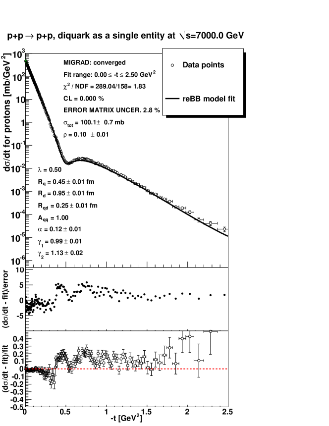
Figure 1: The fit of the ReBB model in the whole $0<|t|<2.5$ GeV² range at $\sqrt{s}=7$ TeV. The fit uses the statistical errors of the data points and the luminosity error of the systematic uncertainty according to Eq. (32). Although the fit quality is not satisfactory, CL $\ll$ 0.1%, the fit looks good by eye. The fitted parameters are shown in the left bottom corner, parameters without errors were fixed during the MINUIT optimization. The total cross-section $\sigma_{tot}$ and the parameter $\rho$ are derived quantities according to Eqs. (11) and (12), respectively. Parameter values are rounded up to two decimal digits. The uncertainty of the MINUIT error matrix after the fit is 2.8 %.

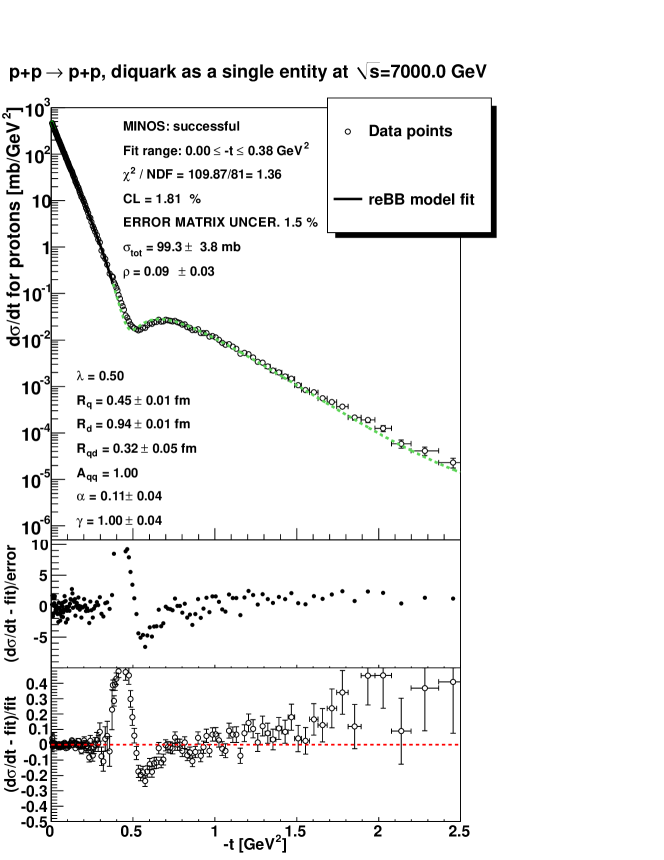
Figure 2: The fit of the ReBB model in the $0<|t|<|t_{sep}|$ range at $\sqrt{s}=7$ TeV. The fit quality is satisfactory, CL $>0.1\%.$ The fit uses the statistical errors of the data points and the luminosity error of the systematic uncertainty according to Eq. (32). The fitted curve is shown with solid line, its extrapolation above $|t_{sep}|$ is indicated with a dashed line. The extrapolated curve remains close to the data points, following the measured differential cross-sections well even far away from the fitted region. The fitted parameters are shown in the left bottom corner, rounded to two valuable decimal digits. The parameters without errors were fixed in the minimization. The total cross-section $\sigma_{tot}$ and the parameter $\rho$ are derived quantities according to Eqs. (11) and (12), respectively. The uncertainty of the MINUIT error matrix after the fit is 1.5 %.

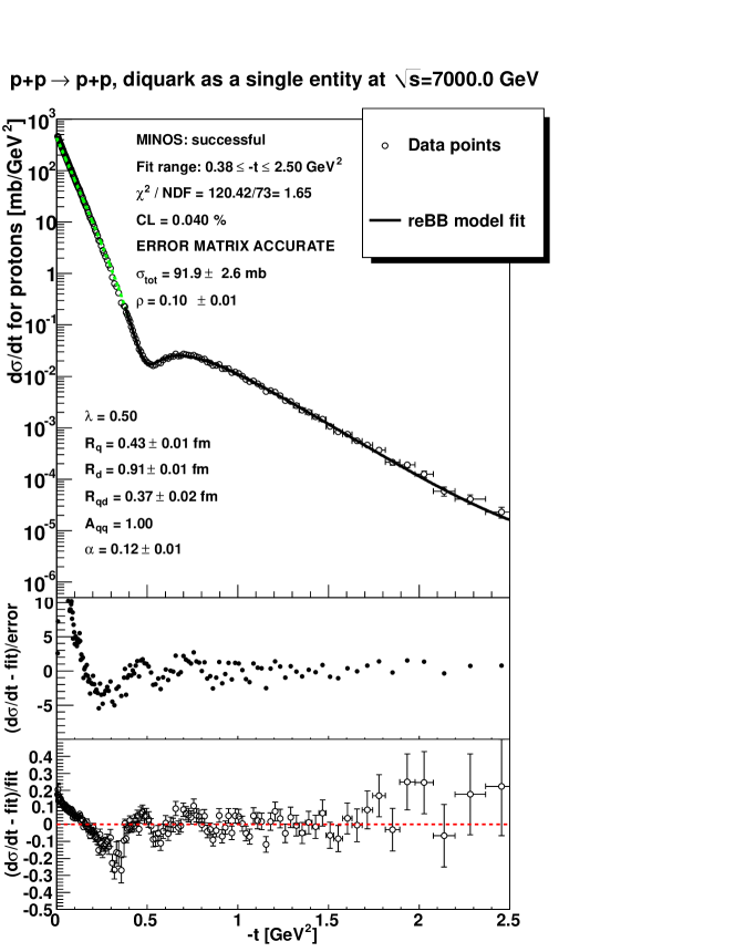
Figure 3: The same as Fig. 2, but the fit is performed in the $|t_{sep}|<|t|<2.5$ GeV² range. The fit uses the statistical errors of the data points and we present the results for the $\gamma=1$ fixed case. The fitted curve is shown with solid line, its extrapolation is indicated with a dashed line. Parameter values are rounded up to two valuable decimal digits. Note that when the curve is extrapolated to the low-$|t|$ region, the extrapolated curve again follows the measured differential cross-section remarkably well even far away the fit region: the ReBB model fit is remarkably stable over the whole $|t|$-range.

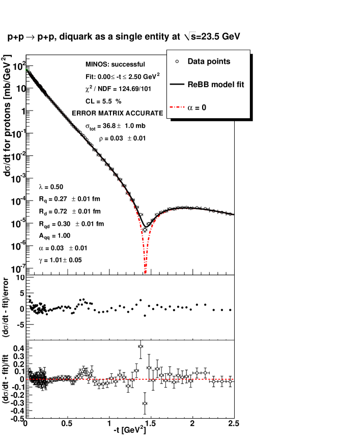
Figure 4: The fit of the ReBB model at $\sqrt{s}=23.5$ GeV in the $0<|t|<2.5$ GeV² squared four-momentum transfer $|t|$ range. The fit uses the statistical errors of the data points and the luminosity error of the systematic uncertainty according to Eq. (32). Parameter values are rounded up to two valuable decimal digits.

If the two parameters $A_{qq}$ and $\lambda$ are released and included into the set of fitted parameters of the ReBB model, the fit quality improves at each analyzed energy from the point of view of mathematical statistics. In case of $\sqrt{s}=30.7$ GeV the improvement is quite significant as the confidence level of the fit reaches $CL=8\,\%$ instead of $2\times 10^{-3}\,\%$. However, the two new fitted parameters introduce more correlations, which lead to large fit uncertainties, and the parameters $\lambda$ and $A_{qq}$ within errors remain in the range of their values that were fixed for the fits reported in Table 1, however, due to the correlations between the fit parameters when $A_{qq}$ and $\lambda$ are released, the fit parameters fluctuate more when evaluated as a function of  $\sqrt{s}$, consequently their trend is more difficult to determine. Therefore, in order to determine the excitation function of the model parameters, we utilized the results of the ReBB fit results as listed in Table 1, where these two parameters $\lambda=1/2$ and $A_{qq}=1$ are fixed.

Also note that if $\text{Im}\,\Omega(s,b)$ is defined to be proportional to $\text{Re}\,\Omega(s,b)$, according to Eq. (31), the MINUIT fit result of $\chi^{2}/NDF=504.9/159=3.2$ is obtained at $\sqrt{s}=7$ TeV in the $0<|t|<2.5$ GeV² range, which is disfavored as compared to fits with Eq. (29), see also Fig. 1.

In our introduction we shortly mentioned the $p=(q,(q,q))$ version of the ReBB model, when the diquark is assumed to be a composition of two quarks [3]. At $\sqrt{s}=7$ TeV in the $0<|t|<2.5$ GeV² range this scenario provides a fit result with $\chi^{2}/NDF=15509/159\approx 97.5$, which means that the $p=(q,(q,q))$ ReBB version can be rejected. The failure of this version is basically due the wrong shape of the differential cross-section: the second diffractive minimum appears too close to the first one.

4 Discussion

4.1 Shadow profile functions and saturation

The fits, from which the model parameters were determined, also permit us to evaluate the shadow profile function

$$A(s,b)=1-\left|\exp\left[-\Omega(s,b)\right]\right|^{2}\,.$$ (33)

The obtained curves to $A(b)$ are shown in Fig. 5. The shadow profile functions at ISR energies exhibit a Gaussian like shape, which smoothly change with the center-of-mass energy $\sqrt{s}$. In this case, the $A(s,b=0)<1$ value indicates that the protons are not completely “black” at the ISR energies, even at their centre they do not scatter with the maximum possible probability per unit area. At the LHC energy of $\sqrt{s}=7$ TeV something new appears: the innermost part of the distribution shows a saturation, which means that around $b=0$ the shadow profile function becomes almost flat and stays close to $A(b)\approx 1$. Consequently, the shape of the shadow profile function $A(b)$ becomes non-Gaussian and somewhat “distorted” with respect to the shapes found at ISR. At the same time, the width of the edge of the shadow profile function $A(b)$, which can be visualized as the proton’s “skin-width”, remains approximately independent of the center-of-mass energy $\sqrt{s}$.

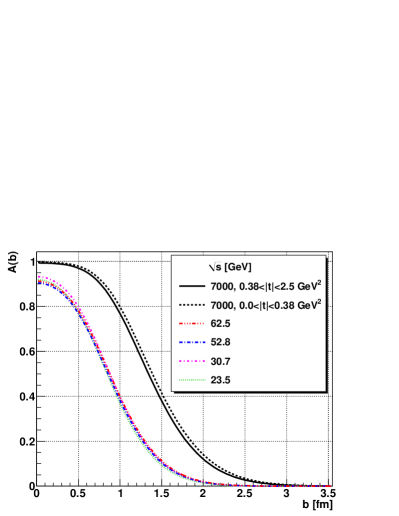
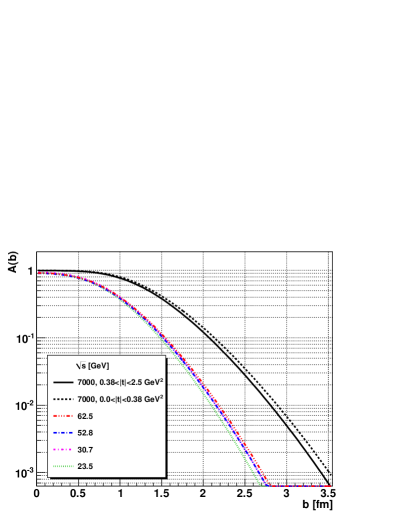
Figure 5: The shadow profile functions $A(b)$ indicate a saturation effect at LHC, while at ISR energies a Gaussian shape can be observed. Note that the 7 TeV (black dashed) curve is based on the statistically acceptable fit result in the $0<|t|<0.38$ GeV² range. The distributions’ edge shows approximately the same width at each energy, corresponding to a constant “skin-width” of the proton.

4.2 Non-exponential behavior of $d\sigma_{el}/dt$

To compare the obtained low-$|t|$ ReBB fit of Fig. 2 with a purely exponential distribution the following exponential parametrization is used

$$\frac{\rm{d}\sigma_{el}}{\rm{d}t}=\left.\frac{\rm{d}\sigma_{el}}{\rm{d}t}\right|_{t=0}\cdot e^{-B\cdot|t|}\,,$$ (34)

where $\left.\rm{d}\sigma_{el}/\rm{d}t\right|_{t=0}=506.4$ mb/GeV² and the slope parameter of $B=19.89$ GeV^-2 is applied, according to the TOTEM paper of Ref. [11].

The result, shown in Fig. 6, indicates a clear non-exponential behavior of the elastic differential cross-section in the $0.0\leq|t|\leq 0.2$ GeV² range at $\sqrt{s}=$7 TeV.

A change of the slope parameter $B(t,s)=({\rm d}/{\rm d}t)\ln({\rm d}\sigma/{\rm d}t)$ around $-t\approx 0.10$ GeV² was reported already in the year 1972 in elastic $pp$ collisions at the ISR energy range of 21.3 $<\sqrt{s}<$ 54 GeV and the 0.02 GeV${}^{2}<-t<$ 0.40 GeV² squared four-momentum transfer range. A very similar structure, a deviation from an exponential behavior was also reported as early as in 1984 in the analysis of proton-antiproton elastic scattering at 546 GeV by Glauber and Velasco [28]. The first preliminary results on such a non-exponential behavior at the CERN LHC energy of 8 TeV were made public recently in $pp$ elastic scattering by the TOTEM experiment at various conference presentations during 2014 [6] and were already interpreted in the theoretical work of Ref. [7], as the consequence of two-pion exchange and $t$-channel unitarity, while Ref. [8], related this $t$ dependence of the slope parameter $B$ to pion loop contribution to the Pomeron trajectory in two-channel eikonal models.

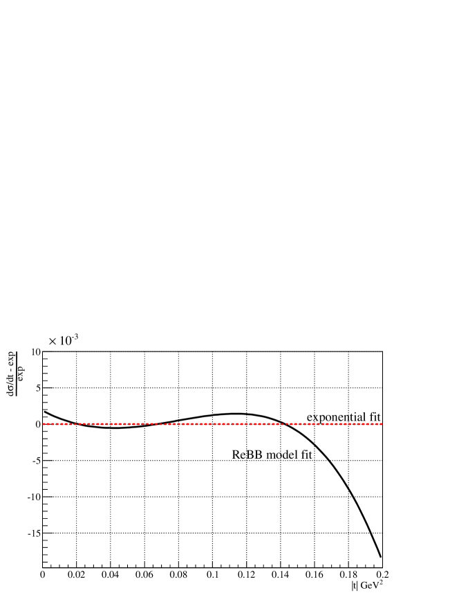
Figure 6: The ReBB model fit result, shown in Fig. 2, with respect to the exponential fit of Eq. (34). In the plot only the $0.0\leq|t|\leq 0.2$ GeV² range is shown, but the ReBB model is fitted to 7 TeV TOTEM data in the low-$t$ interval of $(0,t_{sep})$. The ReBB fit result indicates a significant deviation from the simple exponential at low-$|t|$ values.

5 Extrapolation to future LHC energies and beyond

The ReBB model can be extrapolated to energies which have not been measured yet at LHC. The fit results of Table 1 and the parametrization

$$P(s)=p_{0}+p_{1}\cdot\ln{(s/s_{0})}$$ (35)

is applied for each parameter $P\in{\{R_{q},R_{d},R_{qd},\alpha\}}$, where $s_{0}=1$ GeV². The parametrization Eq. (35) implies that the four free parameters of the original ReBB model that were fitted at each colliding energy independently, corresponding to altogether 20 free fit parameters at the 5 energies analyzed in this manuscript are now replaced with eight parameters $p_{i}$ that prescribe their energy dependence. These fits to the energy dependence of the ReBB model parameters are shown in Fig. 7 and the fit parameters are collected in Table 2.

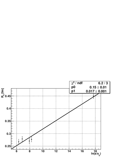
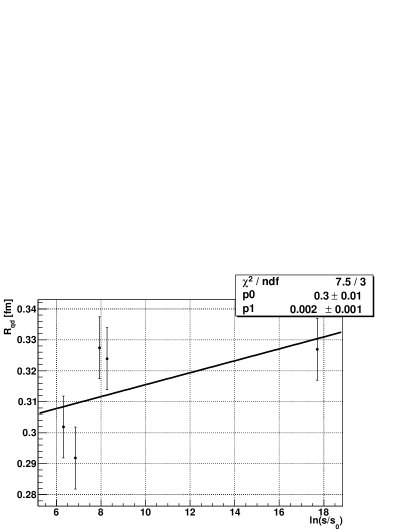
Figure 7: The excitation function of the parameters of the ReBB model, collected in Table 1, is determined from fits with Eq. (35) to each of the parameters $R_{q}$, $R_{d}$, $R_{qd}$ and $\alpha$. The plots about the resulting fits are collected here, while the parameters of the excitation functions are collected in Table 2. The statistically acceptable quality of these fits allow the ReBB model to be extrapolated to center-of-mass energies which have not been measured yet at LHC.

The logarithmic dependence of the geometric parameters on the center-of-mass energy $\sqrt{s}$ in the parametrization Eq. (35) is motivated by the so-called “geometric picture“ based on a series of studies [29, 30, 31, 32, 33, 34]. In case of the $\alpha$ parameter, which is not a geometrical property of the proton, the logarithmic $\sqrt{s}$ dependence is an additional assumption. As indicated by Fig. 7 and Table 2, such an energy dependence of the $\alpha$ shape parameter is consistent with the currently available data.

Table 2 shows that the rate of increase with $\sqrt{s}$, parameter $p_{1}$, is an order of magnitude larger for $R_{q}$ and $R_{d}$ than for $R_{qd}$. The saturation effect, described in Section 4.1, is consistent with this observation as the increasing components of the proton, the quark and the diquark, are confined into a volume which is increasing more slowly.

Parameter	$R_{q}$ [$fm$]	$R_{d}$ [$fm$]	$R_{qd}$ [$fm$]	$\alpha$
$\chi^{2}/NDF$	$6.2/3$	$2.4/3$	$7.5/3$	$1.2/3$
CL [%]	10.2	49.4	5.8	75.3
$p_{0}$	$0.15\pm 0.01$	$0.59\pm 0.01$	$0.30\pm 0.01$	$-0.04\pm 0.01$
$p_{1}$	$0.017\pm 0.001$	$0.019\pm 0.001$	$0.002\pm 0.001$	$\phantom{-}0.009\pm 0.001$

Table 2: The fits of the ReBB model to data at each ISR energy and at the 7 TeV LHC energy, summarized in Table 1, allow for an extrapolation of the model parameters as a function of the center-of-mass energy $\sqrt{s}$. The parametrization Eq. (35) is applied to each parameter of the ReBB model and the fits are shown in Fig. 7. Numerical values are rounded up to two valuable decimal digits. The fit quality information is provided in the first and second row of the table. Note that the fit quality is acceptable for each parameter as CL$>$0.1 % for each fit.

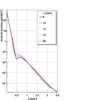
Figure 8: The $pp$ elastic differential cross-section is extrapolated to 8 TeV as well as to future LHC energies and beyond.

Using the extrapolation formula Eq. (35) and the value of the parameters from Table 2 it is straightforward to calculate the values of the parameters at 8 TeV, where the TOTEM measurement of the total cross-section is published [35], and at expected future LHC energies of $\sqrt{s}=$13, 14, 15 TeV and also at 28 TeV, which is beyond the LHC capabilities. Using the extrapolated values of the parameters we plot our predicted $pp$ elastic differential cross-section curves at each mentioned energy in Fig. 8. The shadow profile functions $A(b)$ can be also extrapolated, see Fig. 9. The shadow profile functions even allow us to visualize the increasing effective interaction radius of the proton in the impact parameter space in Fig. 10.

It is also important to see how the most important features change with center-of-mass energy $\sqrt{s}$: the extrapolated values of the total cross-section $\sigma_{tot}$, the position of the first diffractive minimum $|t_{dip}|$ and the parameter $\rho$ is given in Table 3.

Our calculated value at $\sqrt{s}=8$ TeV is $\sigma_{tot}=99.6$ mb, which is consistent with the total cross-section $\sigma_{tot}=101.7\pm 2.9$ mb at $\sqrt{s}=8$ TeV, measured with a luminosity-independent method by the TOTEM experiment [35].

According to Table 3, the predicted value of $|t_{dip}|$ and $\sigma_{tot}$ moves more than 10% when $\sqrt{s}$ increases from 8 TeV to 28 TeV, while the value of $C=|t_{dip}|\cdot\sigma_{tot}$ changes only about 2 %, which is an approximately constant value, within the errors of the extrapolation.

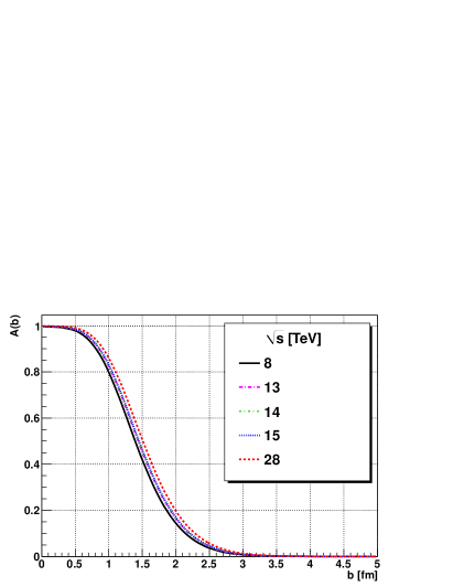
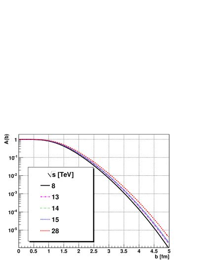
Figure 9: The shadow profile function at the extrapolated energies $\sqrt{s}$. The results show the increase of the proton interaction radius with increasing $\sqrt{s}$ energies. Also note that the “edge” of the distributions remains of approximately constant width and shape.

$\sqrt{s}$ [TeV]	$\sigma_{tot}$ [mb]	$|t_{dip}|$[GeV2]	$\rho$	$|t_{dip}|\cdot\sigma_{tot}$ [mb GeV2]
8	99.6	0.494	0.103	49.20
13	106.4	0.465	0.108	49.48
14	107.5	0.461	0.108	49.56
15	108.5	0.457	0.109	49.58
28	117.7	0.426	0.114	50.14

Table 3: The extrapolated values of the total cross-section $\sigma_{tot}$ at future LHC energies and beyond. The position of the first diffractive minimum $|t_{dip}|$, the parameter $\rho$ and the $|t_{dip}|\cdot\sigma_{tot}$ value is also provided at each energy. Note that the predicted value of $|t_{dip}|$ and $\sigma_{tot}$ moves more than 10% when $\sqrt{s}$ increases from 8 TeV to 28 TeV, while the value of $|t_{dip}|\cdot\sigma_{tot}$ changes only about 2 %.

A similar, and exact, scaling can be derived for the case of photon scattering on a black disk, where the elastic differential cross-section is [36]

$$\frac{d\sigma_{black}}{dt}=\pi R^{4}\left[\frac{J_{1}(q\cdot R)}{q\cdot R}\right]^{2}\,,$$ (36)

where $R$ is the radius of the black disk and $t=-q^{2}$. The total cross-section is given by

$$\sigma_{tot,black}=2\pi R^{2}\,.$$ (37)

In this simple theoretical model the position of the first diffractive minimum, following from Eq. (36), and the total cross-section Eq. (37) satisfies

$$C_{black}=|t_{dip,black}|\cdot\sigma_{tot,black}=2\pi j_{1,1}^{2}(\hbar c)^{2}\approx~{}35.9\,\text{mb GeV}^{2}\,,$$ (38)

where $j_{1,1}$ is the first root of the first order Bessel-function of the first kind $J_{1}(x)$.

The scaling behavior, indicated by the stability of the value $C$, is observed, but it is significantly different from the black disk model, described by Eq. (38), as the corresponding value $C_{black}$ is significantly different

$$C_{black}\neq C\,.$$ (39)

In this sense the value of $C$ indicates a more complex scattering phenomena, than the scattering of a photon on a black disc, however, the constancy of the product suggests the validity of an asymptotic geometric picture, in agreement with the recent observations in Refs. [37, 3, 38, 39].

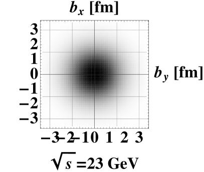
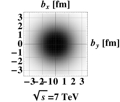
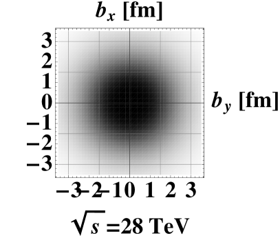
Figure 10: Visualization of the shadow profile functions $A(b)$ in the transverse plane of the impact parameter vector $(b_{x},b_{y})$. The figures show the increase of the proton effective interaction radius in the impact parameter space with increasing center-of-mass energy $\sqrt{s}$. It can be also observed that the black innermost core of the distributions is increasing, while the thickness of the proton’s “skin”, the gray transition part of the distributions, remains approximately independent of the center-of-mass energy $\sqrt{s}$.

6 Summary and conclusions

The real part of the forward scattering amplitude (FSA) is derived from unitarity constraints in the Bialas-Bzdak model leading to the so-called ReBB model. The added real part of the FSA significantly improves the model ability to describe the data at the first diffractive minimum. In total the ReBB model describes both the ISR and LHC data in the $0<|t|<2.5$ GeV² squared four-momentum transfer range in a statistically acceptable manner; in the latter case the fit range has to be divided to two parts, according to the compilation of the two independent TOTEM measurements. The results are collected in Table 1.

The fit results also permit us to evaluate the shadow profile functions $A(b)$, see Fig. 5. The plots indicate a Gaussian shape at ISR energies, while at LHC a saturation effect can be observed: the innermost part of the shadow profile function $A(b)$ around $b=0$ is almost flat and close to $A(b)\approx 1$. The elastic differential cross-section can be compared to a purely exponential distribution and the comparison shows a significant deviation from pure exponential in the $0.0\leq|t|\leq 0.2$ GeV² range.

The fit results allow the determination of the excitation functions of the ReBB model at future LHC energies and beyond, with parameters collected in Table 2 and predicted differential cross-section curves shown in Fig. 8. The shadow profile functions can be also extrapolated, see Fig. 9, which predicts that the saturated part of the proton is expected to increase with increasing center-of-mass energy $\sqrt{s}$. The edge of the distribution, the “skin-width” of the proton, expected to remain approximately constant. It is worth to mention that the extrapolated version of the ReBB model utilizes of only eight parameters, the $p_{i}$ parameters of Table 2, and in this sense a “minimal“ set of parameters is applied.

References

- [1] A. Bialas and A. Bzdak, Acta Phys. Polon. B 38 (2007) 159
- [2] F. Nemes and T. Csörgő, Int. J. Mod. Phys. A 27 (2012) 1250175
- [3] T. Csörgő and F. Nemes, Int. J. Mod. Phys. A 29 (2014) 1450019
-
[4]
E. Ferreira, T. Kodama and A. K. Kohara,
[arXiv:1411.3518 [hep-ph]],
Proc. 8th International Workshop on Diffraction in High Energy Physics (Diffraction 2014), 10-16 Sep 2014. Primosten, Croatia. - [5] A. K. Kohara, E. Ferreira and T. Kodama, Eur. Phys. J. C 74 (2014) 11, 3175
-
[6]
S. Giani, “Overview of TOTEM results on total cross-section, elastic
scattering and diffraction at LHC”, invited talk at the
WPCF 2014 conference, Gyöngyös, Hungary, August 25-29, 2014
https://indico.cern.ch/event/300974/session/2/contribution/34 .
J. Kašpar for the TOTEM Collaboration, TOTEM Status Report, presented at the 117th LHCC Meeting, March 5, 2014,
https://indico.cern.ch/event/301486/session/0/contribution/5/material/slides/0.pdf - [7] L. Jenkovszky and A. Lengyel, arXiv:1410.4106 [hep-ph].
- [8] V. A. Khoze, A. D. Martin and M. G. Ryskin, arXiv:1410.0508 [hep-ph].
- [9] G. Antchev et al. (TOTEM Collaboration), Europhys. Lett. 96 (2011) 21002
- [10] G. Antchev et al. (TOTEM Collaboration), Europhys. Lett. 95 (2011) 41001
- [11] G. Antchev et al. (TOTEM Collaboration), Europhys. Lett. 101 (2013) 21002.
- [12] G. Antchev et al. (TOTEM Collaboration), Europhys. Lett. 101 (2013) 21004.
- [13] J. Orear, Phys. Rev. Lett. 12 (1964) 112.
- [14] D. B. Lichtenberg and L. J. Tassie, Phys. Rev. 155 (1967) 1601.
- [15] V. A. Tsarev, Lebedev Institute Reports, 4 (1979) 12.
- [16] V. M. Grichine, N. I. Starkov and N. P. Zotov, Eur. Phys. J. C 73 (2013) 2, 2320
- [17] V. M. Grichine, Eur. Phys. J. Plus 129 (2014) 112
- [18] R. J. Glauber, Lectures in Theoretical Physics, Vol. 1. Interscience, New York 1959.
- [19] E. Levin, hep-ph/9808486.
- [20] V. A. Khoze, A. D. Martin and M. G. Ryskin, Int. J. Mod. Phys. A, Vol. 30, 1542004 (2015)
- [21] M. G. Ryskin, A. D. Martin and V. A. Khoze, Eur. Phys. J. C 72 (2012) 1937
- [22] M. G. Ryskin, A. D. Martin, V. A. Khoze and A. G. Shuvaev, J. Phys. G 36 (2009) 093001
- [23] A. D. Martin, H. Hoeth, V. A. Khoze, F. Krauss, M. G. Ryskin and K. Zapp, PoS QNP 2012 (2012) 017
- [24] P. Lipari and M. Lusignoli, Eur. Phys. J. C 73, 2630 (2013)
- [25] L. Demortier, CDF note 8661, 1999
- [26] E. Nagy, R. S. Orr, W. Schmidt-Parzefall, K. Winter, A. Brandt, F. W. Busser, G. Flugge and F. Niebergall et al., Nucl. Phys. B 150 (1979) 221.
- [27] U. Amaldi and K. R. Schubert, Nucl. Phys. B 166 (1980) 301.
- [28] R. J. Glauber and J. Velasco, Phys. Lett. B 147, 380 (1984).
- [29] H. Cheng and T. T. Wu, Phys. Rev. Lett. 22 (1969) 666.
- [30] H. Cheng and T. T. Wu, Phys. Rev. 182 (1969) 1852.
- [31] H. Cheng and T. T. Wu, Phys. Rev. 182 (1969) 1868.
- [32] H. Cheng and T.T. Wu, Expanding Protons: Scattering at High Energies , M.I.T. Press, Cambridge, MA (1987)
- [33] C. Bourrely, J. Soffer and T. T. Wu, Phys. Rev. D 19 (1979) 3249.
- [34] C. Bourrely, J. Soffer and T. T. Wu, Int. J. Mod. Phys. A, Vol. 30, 1542006 (2015)
- [35] G. Antchev et al. (TOTEM Collaboration), Phys. Rev. Lett. 111 (2013) 1, 012001.
- [36] M. M. Block, Phys. Rept. 436 (2006) 71
- [37] I. Bautista and J. Dias de Deus, Phys. Lett. B 718, 1571 (2013)
- [38] M. Giordano and E. Meggiolaro, JHEP 1403, 002 (2014)
- [39] V. V. Anisovich, V. A. Nikonov and J. Nyiri, Phys. Rev. D 90, no. 7, 074005 (2014)