On Monotone Drawings of Trees

Abstract

A crossing-free straight-line drawing of a graph is monotone if there is a monotone path between any pair of vertices with respect to some direction. We show how to construct a monotone drawing of a tree with $n$ vertices on an $O(n^{1.5})\times O(n^{1.5})$ grid whose angles are close to the best possible angular resolution. Our drawings are convex, that is, if every edge to a leaf is substituted by a ray, the (unbounded) faces form convex regions. It is known that convex drawings are monotone and, in the case of trees, also crossing-free.

A monotone drawing is strongly monotone if, for every pair of vertices, the direction that witnesses the monotonicity comes from the vector that connects the two vertices. We show that every tree admits a strongly monotone drawing. For biconnected outerplanar graphs, this is easy to see. On the other hand, we present a simply-connected graph that does not have a strongly monotone drawing in any embedding.

1 Introduction

A natural requirement for the layout of a connected graph is that between any source vertex and any target vertex, there should be a source–target path that approaches the target according to some distance measure. A large body of literature deals with problems of this type; various measures have been studied. For example, in a greedy drawing you can find a path to a target vertex by iteratively selecting a neighbor that is closer to the target. In a monotone drawing, the distance between vertices (on the desired source-target path) is measured with respect to their projections on some line, which may be different for any source–target pair. We say that a path $P$ is monotone with respect to a vector $\vec{v}$ if the orthogonal projection of the vertices of $P$ on every line with direction vector $\vec{v}$ appears on the line in the order as induced by $P$. We also refer to $\vec{v}$ as a direction. In strongly monotone drawings, that line is always the line from source to target, and in upward drawings, the line is always the vertical line, directed upwards.

In this paper, we focus on monotone and strongly monotone drawings of trees with additional aesthetic properties such as convexity or small area. Given a tree, we call the edges incident to the leaves leaf edges and all other edges interior edges. Given a straight-line drawing of a tree, we substitute each leaf edge by a ray whose initial part coincides with the edge. The embedding of the tree in the plane defines a combinatorial embedding of the tree, that is, the order of the edges around every vertex. The faces are then specified by this combinatorial embedding as leaf–leaf paths. If the faces of the augmented drawing are realized as convex nonoverlapping (unbounded) polygonal regions, then we call the original drawing a convex drawing. If every region is strictly convex (that is, all interior angles are strictly less than $\pi$), we also call the drawing strictly convex. Note that a strictly convex drawing is also monotone [2, 4], but a monotone drawing is not necessarily convex. Strict convexity forbids vertices of degree 2. When we talk about (strongly) monotone drawings, this always includes the planarity requirement. Otherwise, as Angelini et al. [2] observed, drawing any spanning tree of the given graph in a (strongly) monotone way and inserting the remaining edges would yield a (strongly) monotone drawing of the graph.

Previous Work.

Rao et al. [20] introduced the concept of greedy drawings for a coordinate-based routing algorithm that does not rely on location information. While any 3-connected plane graph has a greedy drawing in the Euclidean plane [17] (even without crossing [7]), this is, unfortunately, not true for trees. Nöllenburg and Prutkin [18] gave a complete characterization for the tree case, which shows that no tree with a vertex of degree 6 or more admits a greedy drawing.

Alamdari et al. [1] studied a subclass of greedy drawings, so-called self-approaching drawings which require that there always is a source–target path such that the distance decreases for any triplet of intermediate points on the edges, not only for the vertices on the path. These drawings are based on the concept of self-approaching curves [15].

Carlson and Eppstein [6] studied convex drawings of trees. They give linear-time algorithms that optimize the angular resolution of the drawings, both for the fixed- and the variable-embedding case. They observe that convexity allows them to pick edge lengths arbitrarily, without introducing crossings.

For monotone drawings, Angelini et al. [2] studied the variable-embedding case. They showed that any $n$-vertex tree admits a straight-line monotone drawing on a grid of size $O(n^{1.6})\times O(n^{1.6})$ (using a BFS-based algorithm) or $O(n)\times O(n^{2})$ (using a DFS-based algorithm). They also showed that any biconnected planar graph has a monotone drawing (using exponential area). Further, they observed that not every planar graph admits a monotone drawing if its embedding is fixed. They introduced the concept of strong monotonicity and showed that there is a drawing of a planar triangulation that is not strongly monotone. Hossain and Rahman [14] improve some of the results of Angelini et al. by showing that every connected planar graph admits a monotone drawing of size $O(n)\times O(n^{2})$ and that such a drawing can be computed in linear time.

Both the BFS- and the DFS-based algorithms of Angelini et al. precompute a set of $n-1$ integral vectors in decreasing order of slope by using two different partial traversals of the so-called Stern–Brocot tree, an infinite tree whose vertices are in bijection with the irreducible positive rational numbers. Such numbers can be seen as primitive vectors in 2D, that is, vectors with pairwise different slopes. Then, both algorithms do a pre-order traversal of the input tree. Whenever they hit a new edge, they assign to it the steepest unused vector. They place the root of the input tree at the origin and draw each edge $(u,v)$ by adding its assigned vector to the position of $u$. They call such tree drawings slope-disjoint. We will not formally define this notion here, but it is not hard to see that it implies monotonicity.

Angelini, with a different set of co-authors [3], investigated the fixed-embedding case. They showed that, on the $O(n)\times O(n^{2})$ grid, every connected plane graph admits a monotone drawing with two bends per edge and any outerplane graph admits a straight-line monotone drawing.

Our contribution.

We present two main results. First, we show that any $n$-vertex tree admits a convex and, hence, monotone drawing on the $O(n^{1.5})\times O(n^{1.5})$ grid (see Section 3). As the drawings of Angelini et al. [2], our drawings are slope-disjoint, but we use a different set of primitive vectors (based on Farey sequences), which slightly decreases the grid size and helps us achieve better angular resolution. (This also works for the BFS-based algorithm of Angelini et al.) Instead of pre-order, we use a kind of in-order traversal (first child – root – other children) of the input tree, which helps us to achieve convexity. Our ideas can be applied to modify the (non-grid) optimal angular resolution algorithm of Carlson and Eppstein [6] such that a drawing on an $O(n^{1.5})\times O(n^{1.5})$ grid is constructed at the expense of missing the optimal angular resolution by a constant factor.

Second, we show that any tree admits a strongly monotone drawing (see Section 4). So far, no positive results have been known for strongly monotone drawings. In the case of proper binary trees, our drawings are additionally strictly convex. For biconnected outerplanar graphs, it is easy to construct strongly monotone drawings. On the other hand, we present a simply-connected planar graph that does not have a strongly monotone drawing in any embedding.

Subsequent Work.

Subsequent to our work, He and He [12] improved the area bound for monotone drawings of trees to $O(n^{1.205})\times O(n^{1.205})$. Other than the drawings of our algorithm, their drawings are not necessarily convex. Their algorithm follows our approach of using Farey sequences to acquire a set of primitive vectors and then computing a slope-disjoint drawing. Recently, the same authors [11] further reduced the area bound to $O(n\log n)\times O(n\log n)$. For triconnected planar graphs, He and He [13] proved that the convex drawings that an algorithm of Felsner [8] places on a grid of size $O(n)\times O(n)$ are even monotone. Note, however, that augmenting a graph that is not triconnected to triconnectivity, running Felsner’s algorithm and then removing the additional edges will, in general, neither yield a convex nor a monotone drawing. Hence, the result for triconnected graphs does not imply any improvement for trees. Very recently, Felsner et al. [9] showed that all 3-connected planar graphs, outerplanar graphs, and 2-trees admit a strongly monotone drawing. Their algorithm for outerplanar graphs utilizes an alternate proof that every tree admits a strongly monotone drawing, but they also achieve convexity.

2 Building Blocks: Primitive Vectors

The following algorithms require a set of integral vectors with distinct directed slopes and bounded length. In particular, we ask for a set of primitive vectors $P_{d}=\{(x,y)\mid\gcd(x,y)\in\{1,d\},0\leq x\leq y\leq d\}$. Our goal is to find the right value of $d$ such that $P_{d}$ contains at least $k$ primitive vectors, where $k$ is a number that we determine later. We can then use the reflections on the lines $x=y$, $y=0$ and $x=0$ to get a sufficiently large set of integer vectors with distinct directed slopes. The edges of the monotone drawings in Section 3 are translates of these vectors; each edge uses a different vector.

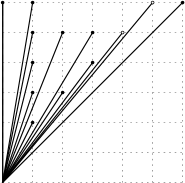
Figure 1: The 13 primitive vectors obtained from $\mathcal{F}_{6}$. The smallest angle of $\approx$ $1.14^{\circ}$ is realized between the vectors $(4,5)$ and $(5,6)$ marked with white dots; the best possible angular resolution in this case is $45^{\circ}/12=3.75^{\circ}$. Note that our algorithm would use $\mathcal{F}_{12}$ to acquire 13 primitive vectors.

Assume that we have fixed $d$ and want to generate the set $P_{d}$. If we consider each entry $(x,y)$ of $P_{d}$ to be a rational number $x/y$ and order these numbers by value, we get the Farey sequence $\mathcal{F}_{d}$ (see, for example, Hardy and Wright’s book [10]). The Farey sequence is well understood. In particular, it is known that $|\mathcal{F}_{d}|=3d^{2}/\pi^{2}+O(d\log d)$ [10, Theorem 331]. Furthermore, the entries of $\mathcal{F}_{d}$ can be computed in time $O(|\mathcal{F}_{d}|)$. We remark that the set $\bigcup_{d}\mathcal{F}_{d}$ coincides with the entries of the Stern–Brocot tree. However, collecting the latter level by level is not the most effective method to build a set of primitive vectors for our purpose.

To obtain a set of $k$ primitive vectors, we use the first $k$ entries of the Farey sequence $\mathcal{F}_{d}$, for $d:=\lceil\pi^{2}\sqrt{k}/3\rceil$, replacing each rational by its corresponding two-dimensional vector. We select exactly $k$ primitive vectors from this set which we denote by $V_{k}$; see Figure 1.

If we wish to have more control over the aspect ratio in our final drawing, we can pick a set of primitive vectors contained inside a triangle spanned by the grid points $(0,0)$, $(m_{x},0),(m_{x},m_{y})$. By stretching the triangle and keeping its area fixed, we may end up with fewer primitive vectors. This will result in an (only slightly) smaller constant compared to the case $m_{x}=m_{y}$. As proven by Bárány and Rote [5, Theorem 2], any such triangular domain contains at least $m_{x}m_{y}/4$ primitive vectors. This implies that we can adapt the algorithm easily to control the aspect ratio by selecting the box for the primitive vectors accordingly. For the sake of simplicity, we detail our algorithms only for the most interesting case ($m_{x}=m_{y}$).

Lemma 1.

Let $P\subseteq P_{d}$ be a set of $k=|P_{d}|/c$ primitive vectors with no coordinate greater than $d$ for some constant $c\geq 1$. Then, any two primitive vectors of $P$ are separated by an angle of $\Omega(1/k)$.

Proof: Since $|P_{d}|=3d^{2}/\pi^{2}+O(d\log d)$, we have that $2d^{2}\approx 2\pi^{2}ck/3$. Any line with slope $m$ encloses an angle $\alpha$ with the $x$-axis, such that $\tan(\alpha)=m$. Let $m_{1}$ and $m_{2}$ be the slopes of two lines and let $\alpha_{1}$ and $\alpha_{2}$ be the corresponding angles with respect to the $x$-axis. By the trigonometric addition formulas we have that the separating angle $\phi$ of these two lines is such that:

$$\tan\phi:=\tan(\alpha_{1}-\alpha_{2})=\frac{\tan\alpha_{1}-\tan\alpha_{2}}{1+\tan\alpha_{1}\tan\alpha_{2}}=\frac{m_{1}-m_{2}}{1+m_{1}m_{2}}.$$

For any two neighboring entries $p/q$ and $r/s$ in the Farey sequence, it holds that $qr-ps=1$ [10, Theorem 3.1.2], and therefore $p/q$ and $r/s$ differ by exactly $(qr-ps)/(qs)=1/(qs)$. Now assume that $\phi$ is the angle between the vectors $(p,q)$ and $(r,s)$. As a consequence, $\tan\phi=1/(pr+qs)$. Then, $\phi$ is minimized if $pr+qs$ is maximized. Clearly, we have that $pr+qs\leq 2d^{2}\approx 2\pi^{2}ck/3$. By the Taylor expansion, $\arctan(x)=x-x^{2}\xi/(1+\xi^{2})^{2}$ for some value $0\leq\xi\leq x$. Substituting $x$ with $3/(2\pi^{2}ck)$ yields, for $k\geq 2$, that

$$\phi\geq\frac{3}{2\pi^{2}ck}-\frac{9\xi}{4\pi^{4}c^{2}k^{2}(1+\xi^{2})^{2}}>\frac{3}{2\pi^{2}ck}-\frac{9}{4\pi^{4}c^{2}k^{2}}\in\Omega(1/k).$$

Since the best possible resolution for a set of $k$ primitive vectors is $2\pi/k$, Lemma 1 shows that the resolution of our set differs from the optimum by at most a constant. To estimate this constant, let us assume we use $k=|P_{d}|$ primitive vectors (that is, $c=1$ in Lemma 1). Then, the smallest angle $\phi$ spanned by these vectors is, according to the proof of the previous lemma, at least $3/(2\pi^{2}k)-9/(16\pi^{4})$ for any $k>1$. This value should be compared to $\text{opt}=\pi/(4k)$ since the primitive vectors span an angle of $\pi/4$ in total. We obtain that the ratio $\phi/\text{opt}$ is smaller than 6.

3 Monotone Grid Drawings with Large Angles

In this section, we present a simple method for drawing a tree on a grid in a strictly convex, and therefore monotone way. Lemma 2 shows that this drawing is automatically crossing-free. We name our strategy the inorder-algorithm. We start by ensuring that convex tree drawings are crossing-free. This has already been stated (without proof) by Carlson and Eppstein [6].

Lemma 2.

Any convex straight-line drawing of a tree is crossing-free.

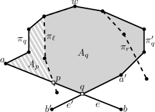
Figure 2: An illustration of the situation in the proof of Lemma 2

Proof.

Let $T$ be a tree and $\Gamma$ a convex straight-line drawing of $T$. Assume that two edges $e=(a,b)$ and $e^{\prime}=(a^{\prime},b^{\prime})$ are crossing in $\Gamma$ in some point $q$, see Figure 2. Let $w$ be the lowest common ancestor of $b$ and $b^{\prime}$, let $\pi_{q}$ be the path $w\to q$ via $a$, and let $\pi_{q}^{\prime}$ the path $w\to q$ via $a^{\prime}$. Let us assume that the children in $w$ are ordered such that $\pi_{q}$ starts before $\pi_{q}^{\prime}$. Let $A_{q}$ be the region bounded by $\pi_{q}$ and $\pi_{q}^{\prime}$.

We can assume that $A_{q}$ is of minimum area with respect to other crossings we may have chosen (and, hence, $A_{q}$ has a connected interior). Now, we consider two paths starting from $w$. The first one, $\pi_{\ell}$, starts with the first edge of $\pi_{q}$ and then always continues via the last child until it reaches a leaf. The second path, $\pi_{r}$, starts with the first edge of $\pi_{q}^{\prime}$ and continues always using the first child. Note that the polygonal chain $\pi_{\ell}$ together with $\pi_{r}$ forms a face $f_{q}$ of the given convex drawing of the tree. Hence, the face is convex, which means that $\pi_{\ell}$ and $\pi_{r}$ only meet in $w$. Furthermore, we either have $\pi_{\ell}\not=\pi_{q}$ or we have $\pi_{r}\not=\pi^{\prime}_{q}$ since otherwise $f_{q}$ is self-intersecting. As a consequence, at least one of the two paths, say $\pi_{\ell}$, enters and leaves $A_{q}$. Let $p$ be the point where $\pi_{\ell}$ crosses $\pi_{q}$ for the first time, and let $A_{p}$ be the polygon that is bounded by the parts of $\pi_{q}$ and $\pi_{\ell}$ between $w$ and $p$. Then $A_{p}$ has smaller area than $A_{q}$, which contradicts our assumption that $A_{q}$ has minimum area. ∎

Our inorder-algorithm first computes a reasonable large set of primitive vectors, then selects a subset of these vectors, and finally assigns the slopes to the edges. The drawing is then generated by translating the selected primitive vectors. In the following, an extended subtree will refer to a subtree including the edge leading into the subtree (if the subtree is not the whole tree).

We will assign a unique number $s(e)$ to every edge $e$. This number will refer to the rank of the edge’s slope (in circular order) in the final assignment. The rank assignment is done in a recursive fashion with increasing integral ranks from $1$ to $n-1$. Starting with the root, for each vertex $v$, we first recursively visit its leftmost child, then assign the next rank to the parent edge of $v$ (unless $v$ is the root), and then recursively visit its other children from left to right. For an example of a tree with its edge ranks, see Figure 3(a).

(a) a tree with edge numbers $s(\cdot)$

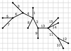
(b) our grid drawing of the tree

Figure 3: A strictly convex drawing of a tree

Second, we assign actual slopes to the edges. Let $e$ be an edge with $s(e)=j$. Then, we assign some vector $s_{j}\in\mathbb{Z}^{2}$ to $e$ and draw $e$ as a translate of $s_{j}$. We pick the vectors $s_{1},s_{2},\dots,s_{n-1}$ by selecting a sufficiently large set of primitive vectors and their reflections in counterclockwise order; see Section 2. Our drawing algorithm has the following requirements:

1. Edges that are incident to the root and consecutive in circular order are assigned to vectors that together span an angle less than $\pi$.

2. In every extended subtree hanging off the root, the edges (including the edge incident to the root) are assigned to a set of vectors that spans an angle less than $\pi$.

These requirements can always be fulfilled, as the following lemma shows.

Lemma 3.

We can select $n-1$ vectors with distinct directed slopes from a $[-d,d]\times[-d,d]$ grid with $d=4\lceil\sqrt{n}\rceil$ such that the requirements R1 and R2 are fulfilled.

Proof.

We first preprocess our tree by adding temporary edges at some leaves. These edges will receive slopes, but are immediately discarded after the assignment.

First, our objective is to ensure that the tree can be split up into three parts that all have $n$ edges. In particular, we adjust the sizes of the extended subtrees hanging off the root by adding temporary edges such that we can partition them into three sets of consecutive extended subtrees which all contain $n$ edges. Note that we have to add $2n+1$ edges to achieve this.

Second, we define three cones $C_{1}$, $C_{2}$, and $C_{3}$; see Figure 4. Each cone has its apex at the origin and spans an angle of $\pi/4$. The angular ranges are $C_{1}=[0,\pi/4]$, $C_{2}=[3\pi/4,\pi]$, and $C_{3}=[3\pi/2,7\pi/4]$; angles are measured from the $x$-axis pointing in positive direction. Note that $C_{2}$ is separated from the two other cones by an angle of $\pi/2$. As mentioned in Section 2, the set $V_{n}$ contains $n$ primitive vectors in the $[0,d]\times[0,d]$ grid. When reflected on the $x=y$ line, these vectors lie in $C_{1}$. Reflecting the vectors in $C_{1}$, we further generate $n$ vectors in $C_{2}$ and $n$ vectors in $C_{3}$. In every cone, we “need” at most $n-3$ edges. Hence, we can remove the vectors on the boundary of each cone. After removing the temporary edges, the number of vectors will drop from $3n$ to $n-1$.

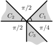
Figure 4: The cones that contain the slopes used in the algorithm

Now, we observe the following. Every two consecutive edges incident to the root lie in the interiors of our cones. Given the sizes and angular distances of the cones, this yields requirement R1. Furthermore, any extended subtree is assigned slopes from a single cone. This yields requirement R2. ∎

For the example tree of Figure 3(a), it suffices to pick the 16 vectors that one gets from reflecting the primitive vectors from the $[0,2]\times[0,2]$ grid. These vectors already fulfill requirements R1 and R2. Hence, we do not have to apply the more involved slope selection as described in Lemma 3. The resulting drawing is shown in Figure 3(b).

Every face in the drawing contains two leaves. The leaves are ordered by their appearance in some DFS-sequence $\mathcal{D}$ respecting some rooted combinatorial embedding of $T$. For a face $f$, we call the leaf that comes first in $\mathcal{D}$ the left leaf and the other leaf of $f$ the right leaf of $f$. The only exception is the face whose leaves are the first and last child of $\mathcal{D}$. Here, we call the first vertex in $\mathcal{D}$ the right leaf and the last vertex in $\mathcal{D}$ the left leaf.

Lemma 4.

Let $u$ be the left leaf, and let $v$ be the right leaf of a face of $T$. Further, let $w$ be the lowest common ancestor of $u$ and $v$. The above assignment of slope ranks $s$ to the tree edges implies the following.

1. If edge $e_{1}$ is on the path $w\to u$ and edge $e_{2}$ is on the path $w\to v$, then $s(e_{1})<s(e_{2})$.

2. The ordered sequence of edges on the path $w\to u$ is increasing in $s(\cdot)$.

3. The ordered sequence of edges on the path $w\to v$ is decreasing in $s(\cdot)$.

Proof.

Let $a$ be an edge that links the parent $p$ to its child $u$, let $b$ be the edge that links $u$ to its leftmost child, and let $c$ be the edge that links $u$ to its rightmost child; see Figure 5(b). In the assignment, we first picked the slope in the subtree rooted at the leftmost children of $u$, then we selected the slope for $a$, and later we picked the slopes for the subtree rooted at the rightmost children of $u$. Since we select the slopes in their radial order, we have $s(b)<s(a)<s(c)$.

Now, note that the slopes on the path $w\to u$ have been assigned before the slopes on the path $w\to v$, which proves (a). When traversing the path $w\to u$, we follow the rightmost children, except maybe for $w$’s child; see Figure 5(a). Hence, the sequence of slopes is increasing, and (b) follows. Statement (c) follows by a similar argument: We traverse the path $w\to v$ by taking the leftmost child, except maybe for $w$’s child. Hence, the sequence of slopes is decreasing. ∎

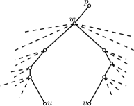
(a) paths spanned by $u,v,w$

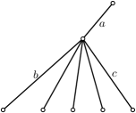
(b) local assignments in the proof

Figure 5: Situation analyzed in Lemma 4

We now prove the correctness of our algorithm.

Theorem 1.

Given an embedded tree with $n$ vertices (none of degree 2), the inorder-algorithm produces a strictly convex and crossing-free drawing with angular resolution $\Omega(1/n)$ on a grid of size $O(n^{1.5})\times O(n^{1.5})$. The algorithm runs in $O(n)$ time.

Proof.

We first show that no face in the drawing is incident to an angle larger than $\pi$. Let $f$ be a face, let $e$ and $e^{\prime}$ be two consecutive edges on the boundary of $f$, and let $\alpha$ be the angle formed by $e$ and $e^{\prime}$ in the interior of $f$. If $e$ and $e^{\prime}$ are incident to the root, requirement R1 implies $\alpha<\pi$. If both edges contain the lowest common ancestor of the leafs belonging to $f$, then, by requirement R2, also $\alpha<\pi$. In the remaining case, $e$ and $e^{\prime}$ both lie on a path to the left leaf of $f$, or both lie on a path to the right leaf of $f$. Let $v$ be the vertex shared by $e$ and $e^{\prime}$. At vertex $v$, we have at least two outgoing edges. Let $e_{1}$ be the first outgoing edge and $e_{2}$ be the last outgoing edge at $v$—one of the edges is $e^{\prime}$. By the selection of the slope ranks, we have $s(e_{1})<s(e)<s(e_{2})$. Consequently, the supporting line of $e$ separates $e_{1}$ and $e_{2}$, and hence both faces containing $e$ have an angle less than $\pi$ at $v$. Therefore, it holds that $\alpha<\pi$.

Next, we show that the edges and rays of a face do not intersect. Then, by Lemma 2, no edges will cross. Assume that there are two edges/rays $\ell$ and $r$ in a common face that intersect in some point $x$. Let $t$ be the lowest common ancestor of $\ell$ and $r$, and assume that $\ell$ lies on the path to the left leaf and $r$ on the path to the right leaf. We define a closed polygonal chain $P$ as follows. The chain starts with the path $t\to\ell$, continues via $x$ to $r$, and finally returns to $t$. We direct the edges according to this walk (for measuring the directed slopes) and call them $e_{1},e_{2},\dots,e_{k}$. We may assume that $P$ is simple; otherwise, we find another intersection point. By Lemma 4, the slopes are monotone when we traverse $P$. For $i=1,\dots,k-1$, let $\alpha_{i}$ be the difference between the directed slopes of the edges $e_{i}$ and $e_{i+1}$. Then, the sum $\sum_{i<k}\alpha_{i}$ equals the angle between the slopes of $e_{1}$ and $e_{k}$. Due to requirement R2, this angle is less than $\pi$. Let $\beta_{i}=\pi-\alpha_{i}$ be the angle between $e_{i}$ and $e_{i+1}$ in $P$, and let $\beta_{0}>0$ be the “interior” angle at $t$. We have that

$$\sum_{0\leq i<k}\beta_{i}=\beta_{0}+\sum_{1\leq i<k}(\pi-\alpha_{i})>0+(k-1)\pi-\pi=(k-2)\pi.$$

This, however, contradicts the fact that the angle sum of the polygon with boundary $P$ is $(k-2)\pi$. Thus, our assumption that two edges/rays cross was invalid.

Since the drawing is assembled from $n-1$ integral vectors whose absolute coordinates are at most $O(\sqrt{n})$, the complete drawing uses a grid of dimension $O(n^{1.5})\times O(n^{1.5})$. Since all vectors are reflections of (a subset of) vectors defined by a Farey sequence with at most $n$ entries, Lemma 1 yields that the angular resolution is bounded by $\Omega(1/n)$. ∎

We conclude this section with comparing our result with the drawing algorithm of Carlson and Eppstein [6]. Their algorithm produces a drawing with optimal angular resolution. It draws trees convex, but, in contrast to our algorithm, not necessarily strictly convex. Allowing parallel leaf edges can have a great impact on the angular resolution. However, our ideas can be applied to modify the algorithm of Carlson and Eppstein. For the leaf edges, their algorithm uses a set of $k$ slopes and picks the slopes such that they are separated by an angle of $2\pi/k$. The slopes of interior edges have either one of the slopes of the leaf edges, or are chosen such that they bisect the wedge spanned by their outermost child edges. However, it suffices to assure that the slope of an interior edge differs from the extreme slopes in the following subtree by at least $2\pi/(2k)$.

We can now modify the algorithm as follows. We pick $2k/8$ primitive vectors and reflect them such that they fill the whole angular space with $2k$ distinct integral vectors. We use every other vector of this set for the leaf edges. For an interior edge, we take any vector from our preselected set whose slope lies in between the extreme slopes of the edges in its subtree. Since we have sufficiently spaced out our set of primitive vectors, we can always find such a vector. Thus, we obtain a drawing on the $O(n^{1.5})\times O(n^{1.5})$ grid. Clearly, the drawing does not have optimal angular resolution. However, since we use $2k$ integral vectors, which have by Lemma 1 an angular resolution of $\Omega(1/k)$, we differ from the best possible angular resolution $2\pi/k$ only by a constant factor. Note that the drawings produced by the algorithm of Carlson and Eppstein do not lie on the grid, that is, they do not compute rational coordinates for the vertices (by design, since otherwise perfect angular resolution cannot be achieved).

(a) tree with two dummy vertices

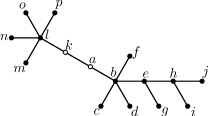
(b) drawing by Carlson and Eppstein [6]

(c) drawing by Angelini et al. [2]

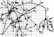
(d) drawing by our algorithm

Figure 6: Example tree of Angelini et al. [2], drawn by various algorithms. We treat the degree-2 vertices as dummy vertices because of the degree restriction.

To conclude this section, we present an example that compares our approach to that of Carlson and Eppstein [6] and to that of Angelini et al. [2]; see Figure 6.

4 Strongly Monotone Drawings

In this section, we show how to draw trees in a strongly monotone fashion. We first show how to draw any proper binary tree, that is, any internal vertex has exactly two children. We name our strategy the disk algorithm. Then, we generalize our result to arbitrary trees. Further, we show that connected planar graphs do not necessarily have a strongly monotone drawing. Finally, we show how to construct strongly monotone drawings for biconnected outerplanar graphs.

Let $T$ be a proper binary tree, let $D$ be any disk with center $c$, and let $C$ be the boundary of $D$. Recall that a strictly convex drawing cannot have a vertex of degree 2. Thus, we consider the root of $T$ a dummy vertex and ensure that the angle at the root is $\pi$. We draw $T$ inside $D$. We start by mapping the root of $T$ to $c$. Then, we draw a horizontal line $h$ through $c$ and place the children of the root on $h\cap\text{int}(D)$ such that they lie on opposite sites relative to $c$. We cut off two circular segments by dissecting $D$ with two vertical lines running through points representing the children of the root. We inductively draw the right subtree of $T$ into the right circular segment and the left subtree into the left circular segment.

In any step of the inductive process, we are given a vertex $v$ of $T$, its position in $D$ (which we also denote by $v$) and a circular segment $D_{v}$; see Figure 7(a). The preconditions for our construction are that

1. $v$ lies in the relative interior of the chord $s_{v}$ that delimits $D_{v}$, and

2. $D_{v}$ is empty, that is, the interiors of $D_{v}$ and $D_{u}$ are disjoint for any vertex $u$ that does not lie on a root–leaf path through $v$.

In order to place the two children $l$ and $r$ of $v$ (if any), we shoot a ray $\vec{v}$ from $v$ perpendicular to $s_{v}$ into $D_{v}$. Let $v^{\prime}$ be the point where $\vec{v}$ hits $C$. Consider the chords that connect the endpoints of $s_{v}$ to $v^{\prime}$. The chords and $s_{v}$ form a triangle with height $vv^{\prime}$. The “height” is contained in the interior of the triangle and splits it into two right subtriangles. The chords are the hypotenuses of the subtriangles. We construct $l$ and $r$ by connecting $v$ to these chords perpendicularly. Note that, since the subtriangles are right triangles, the heights lie inside the subtriangles. Hence, $l$ and $r$ lie in the relative interiors of the chords. Further, note that the circular segments $D_{l}$ and $D_{r}$ delimited by the two chords are disjoint and both are contained in $D_{v}$. Hence, $D_{l}$ and $D_{r}$ are empty, and the preconditions for applying the above inductive process to $r$ and $l$ with $D_{l}$ and $D_{r}$ are fulfilled. See Figure 7(b) for the output of our algorithm for a tree of height 3.

Note that our algorithm does not place the vertices on a grid. However, no edge on a strongly monotone path is perpendicular to its monotone direction. Hence, the vertices can be moved slightly to rational coordinates. Further, the drawings computed by our algorithms require more than polynomial area; in fact, they even require super-exponential area, as the ratio between $s_{v}$ and $s_{l}$ in the inductive step depicted in Figure 7(a) cannot be bounded by a constant. Nöllenburg et al. [19] have recently shown that exponential area is required for strongly monotone drawings of trees, which justifies that we cannot produce a drawing on a grid of polynomial size.

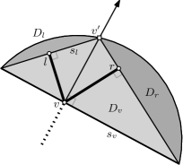
(a) sketch of the inductive step

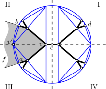
(b) output of our algorithm for a tree of height 3

Figure 7: Strongly monotone drawings of proper binary trees

Lemma 5.

For a proper binary tree rooted in a dummy vertex, the disk algorithm yields a strictly convex drawing.

Proof.

Let $T$ be a proper binary tree and let $f$ be a face of the drawing generated by the algorithm described above. Clearly, $f$ is unbounded. Let $a$ and $b$ be the leaves of $T$ that are incident to the two unbounded edges of $f$, and let $v$ be the lowest common ancestor of $a$ and $b$; see Figure 7(b). Consider the two paths $v\to a$ and $v\to b$. We assume that the path from $v$ through its left child ends in $a$ and the path through its right child ends in $b$.

Due to our inductive construction that uses disjoint disk sections for different subtrees, it is clear that the two paths do not intersect. Moreover, each vertex on the two paths is convex, that is, the angle that such a vertex forms inside $f$ is less than $\pi$. This is due to the fact that we always turn right when we go from $v$ to $a$, and we always turn left when we go to $b$. Vertex $v$ is also convex since the two edges from $v$ to its children lie in the same half-plane (bounded by $s_{v}$).

It remains to show that the two rays $\vec{a}$ and $\vec{b}$ (defined analogously to $\vec{v}$ above) do not intersect. To this end, recall that $v^{\prime}=\vec{v}\cap C$. By our construction, $\vec{a}$ and $\vec{b}$ are orthogonal to two chords of $C$ that are both incident to $v^{\prime}$. Clearly, the two chords form an angle of less than $\pi$ in $v^{\prime}$. Hence, the two rays diverge, and the face $f$ is strictly convex. ∎

For the proof that the algorithm described above yields a strongly monotone drawing, we need the following tools. Let $\vec{v}_{1}$ and $\vec{v}_{2}$ be two vectors. We say that $\vec{v}_{3}$ lies between $\vec{v}_{1}$ and $\vec{v}_{2}$ if $\vec{v}_{3}$ is a positive linear combination of $\vec{v}_{1}$ and $\vec{v}_{2}$. For two vectors $\vec{v}$ and $\vec{w}$, we define $\langle\vec{v},\vec{w}\rangle=|\vec{v}||\vec{w}|\cos(\vec{v},\vec{w})$ as the scalar product of $\vec{v}$ and $\vec{w}$.

Lemma 6.

If a path $p$ is monotone with respect to two vectors $\vec{v}_{1}$ and $\vec{v}_{2}$, then it is monotone with respect to any vector $\vec{v}_{3}$ between $\vec{v}_{1}$ and $\vec{v}_{2}$.

Proof.

Let $\vec{v}_{3}=\lambda_{1}\vec{v}_{1}+\lambda_{2}\vec{v}_{2}$ with $\lambda_{1},\lambda_{2}>0$. Assume that the path $p$ is given by the sequence of vectors $\vec{w}_{1},\vec{w}_{2},\ldots,\vec{w}_{k}$. Since $p$ is monotone with respect to vectors $\vec{v}_{1}$ and $\vec{v}_{2}$, we have that $\langle\vec{v}_{1},\vec{w}_{i}\rangle>0$ and $\langle\vec{v}_{2},\vec{w}_{i}\rangle>0$ for all $i\leq k$. This yields, for all $i\leq k$,

$$\langle\vec{v}_{3},\vec{w}_{i}\rangle=\langle\lambda_{1}\vec{v}_{1}+\lambda_{2}\vec{v}_{2},\vec{w}_{i}\rangle=\lambda_{1}\langle\vec{v}_{1},\vec{w}_{i}\rangle+\lambda_{2}\langle\vec{v}_{2},\vec{w}_{i}\rangle>0,$$

since $\lambda_{1},\lambda_{2}>0$. It follows that $p$ is monotone with respect to $\vec{v}_{3}$. ∎

Lemma 7.

For a proper binary tree rooted in a dummy vertex, the disk algorithm yields a strongly monotone drawing.

Proof.

We split the drawing into four sectors: I, II, III and IV; see Figure 7(b). Let $a$ and $b$ be two vertices in the graph. We will show that the path $a\to b$ in the output drawing of our algorithm is strongly monotone. Let $c$ be the root of the tree. Without loss of generality, assume that $a$ lies in sector III. Then, we distinguish three cases.

Case 1: $a$ and $b$ lie on a common root–leaf path; see $a$ and $v$ in Figure 7(b). Obviously, $b$ lies in sector III. Without loss of generality, assume that $b$ lies on the path $a\to c$. By construction, all edges in sector III, seen as vectors directed towards $c$, lie between $\vec{x}=(0,1)$ and $\vec{y}=(1,0)$. Thus, all edges on the path $a\to b$, and in particular $\vec{ab}$, lie between $\vec{x}$ and $\vec{y}$. Since $\vec{x}$ is perpendicular to $\vec{y}$, the path $a\to b$ is monotone with respect to $\vec{x}$ and $\vec{y}$. Following Lemma 6, the path $a\to b$ is monotone with respect to $\overrightarrow{ab}$, and thus strongly monotone.

Case 2: $b$ lies in sector I; see $a$ and $d$ in Figure 7(b). In Case 1, we have shown that the all edges on the path $a\to c$ lie between $\vec{x}=(0,1)$ and $\vec{y}=(1,0)$. Analogously, the same holds for the path $c\to b$. Thus, the path $a\to b$ is monotone with respect to $\vec{x}$ and $\vec{y}$ and, following Lemma 6, strongly monotone.

Case 3: $a$ and $b$ do not lie on a common root–leaf path, and $b$ does not lie in sector I; see $a$ and $b$ in Figure 7(b). Let $d$ be the lowest common ancestor of $a$ and $b$. Let $\langle a=a_{0},a_{1},\dots,a_{k}=d\rangle$ be the path $d\to a$ to $a$. Further, let $\langle d=b_{0},b_{1},\dots,b_{m}=b\rangle$ be the path $d\to b$. Finally, let $p=\langle a_{k},a_{k-1},\dots,a_{0},b_{1},\dots,b_{m-1},b_{m}\rangle$ be the path $a\to b$.

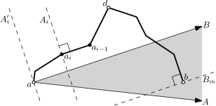
Figure 8: Illustration of case 3 in the proof of Lemma 7

Below, we describe how to rotate and mirror the drawing such that any vector $\overrightarrow{a_{i}a_{i-1}}$ with $1\leq i\leq k$ lies between $\vec{x}=(0,1)$ and $\vec{y}=(1,0)$, and any vector $\overrightarrow{b_{j-1}b_{j}}$ with $1\leq j\leq m$ lies between $\vec{x}$ and $-\vec{y}$. This statement is equivalent to $x(a_{i})<x(d)<x(b_{j}),1\leq i\leq k,1\leq j\leq m$ and $y(a_{k})<\ldots<y(a_{1})<y(d)>y(b_{1})>\ldots>y(b_{m})$; see Figure 8. If $b$ lies in sector IV, then $d=c$ and this statement is true by construction. If $b$ lies in sector II, then $d$ is a child of $c$. We rotate the drawing by $\pi/2$ in counterclockwise direction and then mirror it horizontally. If $b$ lies in sector III, let $p(d)$ be the parent of $d$. We rotate the drawing such that the edge $(p(d),d)$ is drawn vertically. Recall that, by construction, the ray from $d$ in direction $\overrightarrow{p(d)d}=-\vec{y}$ separates the subtrees of the two children of $d$; see Figure 7(a). Further, the angle between any edge (directed away from $d$) in the subtree of $d$ and $\overrightarrow{p(d)d}=-\vec{y}$ is at most $\pi/2$, that is, they are directed downwards.

For $1\leq i\leq k$, let $A_{i}$ be the straight line through $a_{i}$ perpendicular to $\overrightarrow{a_{i-1}a_{i}}$. Let $A^{\prime}_{i}$ be the line parallel to $A_{i}$ that passes through $a$. Due to the $x$-monotonicity of $p$, the point $a$ lies below $A_{i}$. During the construction of the tree, the line $A_{i}$ defined a circular sector in which the subtree rooted at $a_{i}$ including $a$ was exclusively drawn. It follows that $a$ and $b$ lie on opposite sites of $A_{i}$. Thus, $b$ lies above $A_{i}$ and also above $A^{\prime}_{i}$. Let $B_{j},1\leq j\leq m$ be the straight line through $b_{j}$ perpendicular to $\overrightarrow{b_{j-1}b_{j}}$. Let $B^{\prime}_{j}$ be the parallel line to $B_{j}$ that passes through $a$. By construction, $b$ lies below $B_{j}$ and $a$ lies above $B_{j}$. Thus, $b$ lies below $B_{j}^{\prime}$.

Let $A$ be the line $A_{i}^{\prime}$ with maximum slope and let $B$ be the line $B_{j}^{\prime}$ with minimum slope. First, we will show that the path is monotone with respect to the unit vector $\vec{A}$ on $A$ directed to the right. By our choice of $A$, the angle between $\vec{A}$ and any vector $\overrightarrow{a_{i}a_{i-1}}$ with $1\leq i\leq k$ is at most $\pi/2$. Recall that any vector $\overrightarrow{a_{i}a_{i-1}}$ with $1\leq i\leq k$ lies between $\vec{x}$ and $\vec{y}$. Since $\vec{A}$ is perpendicular to one of these edges and directed to the right, it lies between $\vec{x}$ and $-\vec{y}$. Since any vector $\overrightarrow{b_{j-1},b_{j}}$ with $1\leq j\leq m$ also lies between $\vec{x}$ and $-\vec{y}$, the angle between $\vec{A}$ and any such vector $\overrightarrow{b_{j-1},b_{j}}$ is also at most $\pi/2$. Thus, the angle between $\vec{A}$ and any edge on the path $a\to b$ is at most $\pi/2$, which shows that the path is monotone with respect to $\vec{A}$.

Analogously, it can be shown that the path is monotone with respect to $\vec{B}$. Recall that $b$ lies above $A$ and below $B$ and that $a$ lies above $B$ and below $A$. Hence, the vector $\overrightarrow{ab}$ lies between $\vec{A}$ and $\vec{B}$. Following Lemma 6, the path is monotone with respect to $\overrightarrow{ab}$ and, thus, strongly monotone. ∎

Lemmas 5 and 7 immediately imply the following.

Theorem 2.

Any proper binary tree rooted in a dummy vertex has a strongly monotone and strictly convex drawing.

Next, we (partially) extend this result to arbitrary trees.

Theorem 3.

Any tree has a strongly monotone drawing.

Proof.

Let $T$ be a tree. If $T$ has a vertex of degree 2, we root $T$ in this vertex. Otherwise, we subdivide any edge by creating a vertex of degree 2, which we pick as root. Then, we add a leaf to every vertex of degree 2, except the root. Now, let $v$ be a vertex with out-degree $k>2$. Let $(v,w_{1}),\dots,(v,w_{k})$ be the outgoing edges of $v$ ordered from right to left. We substitute $v$ by a path $\langle v=v_{1},\dots,v_{k+1}\rangle$, where $v_{i+1}$ is the left child of $v_{i}$, for $i=1,\dots,k$. Then, we substitute the edges $(v,w_{i})$ by $(v_{i},w_{i}),i=2,\dots,k$; see Figure 9.

(a) a tree $T$

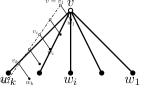
(b) the subdivided tree $T^{\prime}$

Figure 9: Subdivision of a vertex $v$ with $k$ outgoing edges

Let $T^{\prime}$ be the resulting binary tree. Clearly, all vertices of $T^{\prime}$, except its root, have degree 1 or 3, so $T^{\prime}$ is a proper binary tree. We use Theorem 2 to get a strongly monotone drawing $\Gamma_{T^{\prime}}$ of $T^{\prime}$. Then, we remove the dummy vertices inserted above and draw as straight-line segments the edges of the original tree $T$ that have been substituted or subdivided. This yields a drawing $\Gamma_{T}$ of $T$ that is crossing-free since the only new edges form a set of stars that are drawn in disjoint areas of the drawing.

Now, we show that $\Gamma_{T}$ is strongly monotone. Let $(v,w)$ be an edge in $T$. Let $p=\langle v=v_{1},\dots,v_{m}=w\rangle$ be the path $v\to w$ in $T^{\prime}$. Suppose $p$ is monotone with respect to some direction $\vec{d}$. Thus, $\angle\{\overrightarrow{v_{i}v_{i+1}},\vec{d}\}<\pi/2$ for $1\leq i\leq m-1$. Clearly, $\overrightarrow{vw}=\sum_{i=1}^{m-1}\overrightarrow{v_{i}v_{i+1}}$ is a positive linear combination of $\overrightarrow{v_{1}v_{2}},\dots,\overrightarrow{v_{m-1}v_{m}}$ and, hence, $\angle\{\overrightarrow{vw},\vec{d}\}<\pi/2$. It follows that the path $a\to b$ for some vertices $a,b$ in $T$ is monotone with respect to a direction $\vec{d}$ in $\Gamma_{T}$ if the path $a\to b$ is monotone to $\vec{d}$ in $\Gamma_{T^{\prime}}$. With $\vec{d}=\overrightarrow{ab}$, it follows that $\Gamma_{T}$ is strongly monotone. ∎

We add to this another positive result concerning biconnected outerplanar graphs.

Theorem 4.

Any biconnected outerplanar graph has a strongly monotone and strictly convex drawing on the $O(n^{3/2})\times O(n^{3/2})$ grid.

Proof.

Let $G$ be a biconnected outerplanar graph with outer cycle $\langle v_{1},\dots,v_{n},v_{1}\rangle$. We place the vertices $v_{1},\dots,v_{n}$ in order on an $x$- and $y$-monotone convex chain $C$ that has $v_{1}$ and $v_{n}$ as its endpoints. The chain is assembled by translations of $n-1$ primitive vectors, which are sorted by slope (see Figure 11 for a sketch). Since the outer cycle is drawn strictly convex, the drawing is planar and strictly convex. Also, every vector $\overrightarrow{v_{i}v_{j}},j>i$ lies between $\vec{x}=(0,1)$ and $\vec{y}=(1,0)$. Thus, by Lemma 6, the drawing is strongly monotone.

For our construction we can use a set of primitive vectors whose coordinates are bounded by $O(\sqrt{n})$. Since we have linked $n$ such vectors, the asserted bound follows. ∎

We close with a negative result. Angelini et al. [2, p. 33] stated that they are “not aware of any planar graph not admitting a planar monotone drawing for any of its embeddings”. We give the first family of graphs that do not admit any strongly monotone drawing. Note that the graphs in the family that we construct are neither outerplanar nor biconnected.

Theorem 5.

There is an infinite family of connected planar graphs that do not have a strongly monotone drawing in any combinatorial embedding.

Proof.

Let $C$ be the graph that arises by attaching to each vertex of $K_{4}$ a “leaf”; see Figure 11.

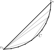
Figure 10: A strongly monotone drawing of a biconnected outerplanar graph

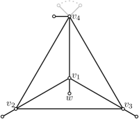
Figure 11: A planar graph without any strongly monotone drawing

Let $v_{1},\dots,v_{4}$ be the vertices of $K_{4}$. For $K_{4}$ to be crossing-free, one of its vertices, say $v_{1}$, lies in the interior. Let $w$ be the leaf incident to $v_{1}$. Because of planarity, $w$ has to be placed inside a triangular face incident to $v_{1}$. Without loss of generality, assume that $w$ is placed in the face $(v_{1},v_{2},v_{3})$. If the drawing is strongly monotone, then $\angle(\overrightarrow{wv_{2}},\overrightarrow{wv_{1}})<\pi/2$ and $\angle(\overrightarrow{wv_{1}},\overrightarrow{wv_{3}})<\pi/2$, and thus $\angle(\overrightarrow{wv_{3}},\overrightarrow{wv_{2}})>\pi$. However, this means that $w$ does not lie inside the triangle $(v_{1},v_{2},v_{3})$, which is a contradiction to the assumption. Thus, $C$ does not have a strongly monotone drawing in any combinatorial embedding. We create an infinite family from $C$ by adding more leaves to the vertices of $K_{4}$. ∎

5 Conclusion

We have shown that any tree has a convex monotone drawing on a grid with area $O(n^{3})$ and a strongly monotone drawing, but several problems remain open. It is an open question whether any tree has a strongly monotone drawing on a grid of exponential size. We have shown that not every connected planar graph admits a strongly monotone drawing, while Felsner et al. [9] showed that every triconnected planar graph does so. It is still open whether there is a biconnected planar graph that does not have any strongly monotone drawing. If yes, it is interesting whether this can be tested efficiently.

References

- [1] S. Alamdari, T. M. Chan, E. Grant, A. Lubiw, and V. Pathak. Self-approaching graphs. In W. Didimo and M. Patrignani, editors, Proc. 20th Int. Symp. Graph Drawing (GD’12), volume 7704 of Lecture Notes Comput. Sci., pages 260–271. Springer, 2013. doi:10.1007/978-3-642-36763-2_23.
- [2] P. Angelini, E. Colasante, G. D. Battista, F. Frati, and M. Patrignani. Monotone drawings of graphs. J. Graph Algorithms Appl., 16(1):5–35, 2012. doi:10.7155/jgaa.00249.
- [3] P. Angelini, W. Didimo, S. G. Kobourov, T. Mchedlidze, V. Roselli, A. Symvonis, and S. K. Wismath. Monotone drawings of graphs with fixed embedding. Algorithmica, 71(2):233–257, 2015. doi:10.1007/s00453-013-9790-3.
- [4] E. M. Arkin, R. Connelly, and J. S. Mitchell. On monotone paths among obstacles with applications to planning assemblies. In K. Mehlhorn, editor, Proc. 5th Ann. ACM Symp. Comput. Geom. (SoCG’89), pages 334–343. ACM, 1989. doi:10.1145/73833.73870.
- [5] I. Bárány and G. Rote. Strictly convex drawings of planar graphs. Doc. Math., 11:369–391, 2006. URL: http://emis.um.ac.ir/journals/DMJDMV/vol-11/13.pdf.
- [6] J. Carlson and D. Eppstein. Trees with convex faces and optimal angles. In M. Kaufmann and D. Wagner, editors, Proc. 14th Int. Symp. Graph Drawing (GD’06), volume 4372 of Lecture Notes Comput. Sci., pages 77–88. Springer, 2007. doi:10.1007/978-3-540-70904-6_9.
- [7] R. Dhandapani. Greedy drawings of triangulations. Discrete Comput. Geom., 43(2):375–392, 2010. doi:10.1007/s00454-009-9235-6.
- [8] S. Felsner. Convex drawings of planar graphs and the order dimension of 3-polytopes. Order, 18(1):19–37, 2001. doi:10.1023/A:1010604726900.
- [9] S. Felsner, A. Igamberdiev, P. Kindermann, B. Klemz, T. Mchedlidze, and M. Scheucher. Strongly monotone drawings of planar graphs. In S. Fekete and A. Lubiw, editors, Proc. 32nd Int. Symp. Comput. Geom. (SoCG’16), 2016. To appear.
- [10] G. Hardy and E. M. Wright. An Introduction to the Theory of Numbers. Oxford Univ. Press, 5th edition, 1979.
- [11] D. He and X. He. Nearly optimal monotone drawing of trees. Theoretical Computer Science, 2016. To appear. doi:http://dx.doi.org/10.1016/j.tcs.2016.01.009.
- [12] X. He and D. He. Compact monotone drawing of trees. In D. Xu, D. Du, and D. Du, editors, Proc. 21st Int. Conf. Comput. Comb. (COCOON’15), volume 9198 of Lecture Notes Comput. Sci., pages 457–468. Springer, 2015. doi:10.1007/978-3-319-21398-9_36.
- [13] X. He and D. He. Monotone drawings of 3-connected plane graphs. In N. Bansal and I. Finocchi, editors, Proc. 23rd Europ. Symp. Algorithms (ESA’15), volume 9294 of Lecture Notes Comput. Sci., pages 729–741. Springer, 2015. doi:10.1007/978-3-662-48350-3_61.
- [14] M. I. Hossain and M. S. Rahman. Monotone grid drawings of planar graphs. In J. Chen, J. E. Hopcroft, and J. Wang, editors, Proc. 8th Int. Workshop Front. Algorithmics (FAW’14), volume 8497 of Lecture Notes Comput. Sci., pages 105–116. Springer, 2014. doi:10.1007/978-3-319-08016-1_10.
- [15] C. Icking, R. Klein, and E. Langetepe. Self-approaching curves. In Math. Proc. Camb. Philos. Soc., volume 125, pages 441–453. Camb. Univ. Press, 1995. doi:10.1017/S0305004198003016.
- [16] P. Kindermann, A. Schulz, J. Spoerhase, and A. Wolff. On monotone drawings of trees. In C. Duncan and A. Symvonis, editors, Proc. 22nd Int. Symp. Graph Drawing (GD’14), volume 8871 of Lecture Notes Comput. Sci., pages 488–500. Springer, 2014. doi:10.1007/978-3-662-45803-7_41.
- [17] T. Leighton and A. Moitra. Some results on greedy embeddings in metric spaces. Discrete Comput. Geom., 44(3):686–705, 2010. doi:10.1007/s00454-009-9227-6.
- [18] M. Nöllenburg and R. Prutkin. Euclidean greedy drawings of trees. In H. L. Bodlaender and G. F. Italiano, editors, Proc. 21st Europ. Symp. Algorithms (ESA’13), volume 8125 of Lecture Notes Comput. Sci., pages 767–778. Springer, 2013. doi:10.1007/978-3-642-40450-4_65.
- [19] M. Nöllenburg, R. Prutkin, and I. Rutter. On self-approaching and increasing-chord drawings of 3-connected planar graphs. In C. Duncan and A. Symvonis, editors, Proc. 22nd Int. Symp. Graph Drawing (GD’14), volume 8871 of Lecture Notes Comput. Sci., pages 476–487. Springer, 2014. doi:10.1007/978-3-662-45803-7_40.
- [20] A. Rao, S. Ratnasamy, C. H. Papadimitriou, S. Shenker, and I. Stoica. Geographic routing without location information. In D. B. Johnson, A. D. Joseph, and N. H. Vaidya, editors, Proc. 9th Ann. Int. Conf. Mob. Comput. Netw. (MOBICOM’03), pages 96–108. ACM, 2003. doi:10.1145/938985.938996.