From the “blazar sequence” to unification of blazars and radio galaxies

Abstract

Based on a large Fermi blazar sample, the blazar sequence (synchrotron peak frequency $\nu_{\rm peak}$ versus synchrotron peak luminosity $L_{\rm peak}$) is revisited. It is found that there is significant anti-correlation between $\nu_{\rm peak}$ and $L_{\rm peak}$ for blazars. However, after being Doppler corrected, the anti-correlation disappears. The jet cavity power ($P_{\rm jet}$) is estimated from extended radio luminosity. So it is free of beaming effect. We find that there are significant anti-correlations between $P_{\rm jet}$ and beam-corrected $\nu_{\rm peak}^{{}^{\prime}}$ for both blazars and radio galaxies, which supports the blazar sequence and unification of blazars and radio galaxies (an alternative relationship is the correlation between jet power and $\gamma$-ray photon index).

1 Introduction

Blazars are the most extreme and powerful active galactic nuclei (AGN), pointing their jets in the direction of the observer (Urry & Padovani 1995; Ghisellini & Tavecchio 2015). Based on the equivalent width (EW) of the emission lines, the blazars are often divided into two subclasses of BL Lacertae objects (BL Lacs; rest frame EW$<5$ Å) and flat spectrum radio quasars (FSRQs; Urry & Padovani 1995). Ghisellini et al. (2009, 2011) introduced a physical distinction between the two classes of blazars, based on the luminosity of the broad line region measured in Eddington units. Giommi et al. (2012, 2013) suggested that blazars should be divided into high and low ionization sources. Their broadband spectral energy distributions (SEDs) are usually bimodal. The lower bump peaks at IR-optical-UV band and the higher bump at GeV-TeV gamma-ray band (Ghisellini et al. 1998; Abdo et al. 2010b).

Fossati et al. (1998) presented the blazar sequence: the peak luminosity of the synchrotron component ($L_{\rm peak}$) and the Compton dominance (the ratio of the peak of the Compton to the synchrotron peak luminosity) are anti-correlation with the synchrotron peak frequency $\nu_{\rm peak}$. Ghisellini et al. (1998) modeled the broadband spectra of blazars, and suggested that along the blazar sequence (BL Lacs $\rightarrow$ FSRQs), a stronger radiative cooling causes a particle energy distribution with a break at lower energies. So the synchrotron and Compton peaks shift to lower frequencies. Various lines of evidence support the blazar sequence (Georganopoulos et al. 2001; Cavaliere & D’Elia 2002; Maraschi & Tavecchio 2003; Xie et al. 2007; Maraschi et al. 2008; Ghisellini & Tavecchio 2008; Ghisellini et al. 2009, 2010; Abdo et al. 2010a; Chen & Bai 2011; Sambruna et al. 2010; Finke et al. 2013; Chen 2014). But many contrary opinions have been presented (Giommi, Menna & Padovani 1999; Caccianiga & Marcha 2004; Padovani et al. 2003; Anton & Browne 2005; Nieppola et al. 2006, 2008; Padovani 2007; Giommi et al. 2012). The authors mainly focus on sample selection effect and beaming effect. Ghisellini & Tavecchio (2008) revisited the blazar sequence and proposed that the SED of blazar emission are linked to the mass of black hole and the accretion rate. Finke (2013) studied a sample of blazars from 2LAC (Ackermann et al. 2011) and found that a correlation exists between Compton dominance and the peak frequency of the synchrotron component for all blazars, including ones with unknown redshift. And via constructing a model, Finke (2013) reproduced the trends of the blazar sequence. Meyer et al. (2011) revisited the blazar sequence and proposed the blazar envelope: FR I radio galaxies (FR Is) and most BL Lacs belong to weak jet population while low synchrotron peaking blazars and FR II radio galaxies (FR IIs) are strong jet population.

Many evidences support that FR IIs are the parent population of FSRQs, and FR Is are the parent population of BL Lacs (Urry & Padovani 1995). It is believed that the unification is mainly due to relativistic beaming. Compared with blazars, radio galaxies is less beaming with a larger jet angle to the line of sight. Fanaroff & Riley (1974) separated radio galaxies into two subclasses with different morphology: the peak of low luminosity FR Is is close to the nucleus, while high luminosity FR IIs have radio lobes with prominent hot spots and bright outer edges. The distinction of morphology also translates into a separation in radio power (the fiducial luminosity $L_{\rm 178}\approx 2\times 10^{25}~{}{\rm W~{}Hz^{-1}}$). Ledlow & Owen (1994) found that the FR Is and FR IIs break depends on radio and optical luminosity. In addition to host galaxy magnitude and environments, FR Is and FR IIs differ in optical emission lines (e.g. Zirbel & Baum 1995). As in the case of blazars, Ghisellini & Celotti (2001) introduced that the division between FR Is and FR IIs actually reflected a systematic difference in accretion rate.

In this paper, after removing beaming effect, we revisited the blazar sequence, and made use of the correlation between jet cavity power and $\nu_{\rm peak}$ to study the unification of blazars and radio galaxies. The paper is structured as follows: in Sect. 2, we present the samples; the results are presented in Sect. 3; discussions and conclusions are presented in Sect. 4. The cosmological parameters $H_{\rm 0}=70~{}{\rm km~{}s^{-1}~{}Mpc^{-1}}$, $\Omega_{\rm m}=0.3$ and $\Omega_{\rm\Lambda}=0.7$ have been adopted in this work.

2 The samples

Our sample was collected directly from sample of Nemmen et al. (2012). But some blazars in Nemmen et al. (2012) were not clean Fermi blazars (2LAC; Ackermann et al. 2011). We removed the non-clean blazars. Generally, the SED was fitted by using a simple third-degree polynomial function. However, many blazars were lack of observed SED. Abdo et al. (2010b) have conducted a detailed investigation of the broadband spectral properties of the $\gamma$-ray selected blazars of the Fermi LAT Bright AGN Sample (LBAS). They assembled high-quality and quasi-simultaneous SED for 48 LBAS blazars, and their results had been used to derive empirical relationships that estimate the position of the two peaks from the broadband colors (i.e. the radio to optical, $\alpha_{\rm ro}$, and optical to X-ray, $\alpha_{\rm ox}$, spectral slopes) and from the $\gamma$-ray spectral index. From 2LAC, we collected the $\alpha_{\rm ro}$ and $\alpha_{\rm ox}$. Then from the empirical relationships of Abdo et al. (2010b), we calculated the $\nu_{\rm peak}$ and corrected redshift for the $\nu_{\rm peak}$. We excluded the blazars without $\alpha_{\rm ox}$. At the same time, using another empirical formula of Abdo et al. (2010b), we estimated the synchrotron peak flux from 5 GHz flux and $\nu_{\rm peak}$. The 5 GHz flux is assembled from NASA/IPAC Extragalactic Database: NED. When more than one flux was found, we took the most recent one. The flux is K-corrected according to $S_{\rm\nu}=S^{\rm{obs}}_{\rm\nu}(1+z)^{{\rm\alpha-1}}$, where $\alpha$ is the spectral index and $\alpha=0.0$. The luminosity is calculated from the relation $L_{\rm\nu}=4\pi{d_{\rm L}}^{2}S_{\rm\nu}$, and $d_{\rm L}$ is the luminosity distance. From Nemmen et al. (2012), for Fermi blazars, $f_{\rm b}$ is the beaming factor ($f_{\rm b}=1-{\rm cos}(1/\Gamma$)), where $\Gamma$ is the bulk Lorentz factor of the flow, since blazars obey $\theta_{\rm j}<1/\Gamma$ (Jorstad et al. 2005; Pushkarev et al. 2009). Pushkarev et al. (2009) calculated the variability Lorentz factors $\Gamma_{\rm var}$ from long-term radio observation. The bulk Lorentz factors of Nemmen et al. (2012) were collected from the results of Pushkarev et al. (2009) (the number $\sim$20%). For blazars without $\Gamma_{\rm var}$ obtained from Pushkarev et al. (2009), they used the power-law fit of $f_{\rm b}\approx 5\times 10^{-4}(L^{\rm obs}_{\rm 49})^{-0.39\pm 0.15}$ as an estimator for $f_{b}$ (significant level at the 3.6$\sigma$; $L^{\rm obs}_{\rm 49}$ is observation $\gamma$-ray luminosity). Moreover, making use of the relation between cavity power and extended radio 300 MHz luminosity and assuming $P_{\rm jet}=P_{\rm cav}$, they estimated the jet kinetic power. So the jet power is free of beaming effect. The uncertainty of jet kinetic power is 0.7 dex. Our beaming factor (or bulk Lorentz factor) and jet kinetic power of blazars are obtained from Nemmen et al. (2012). For radio galaxies, we included the complete radio galaxies sample of Meyer et al. (2011). The $\nu_{\rm peak}$ and $L_{\rm peak}$ of Meyer et al. (2011) were estimated by fitting non-simultaneous average SED. The jet power of Meyer et al. (2011) was calculated from cavity power as same as Nemmen et al. (2012). The relevant data for Fermi blazars were listed in Table 1 and for radio galaxies in Table 3 of Meyer et al. (2011).

In total, we have a sample containing 184 clean Fermi blazars (98 FSRQs and 86 BL Lacs) and 41 radio galaxies (24 FR Is and 17 FR IIs).

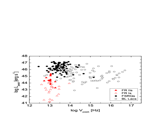
Figure 1: synchrotron peak luminosity versus synchrotron peak frequency. Fermi BL Lacs: black empty circles; Fermi FSRQs: black filled circles; FR I radio galaxies: red empty triangles; FR II radio galaxies: red filled triangles.

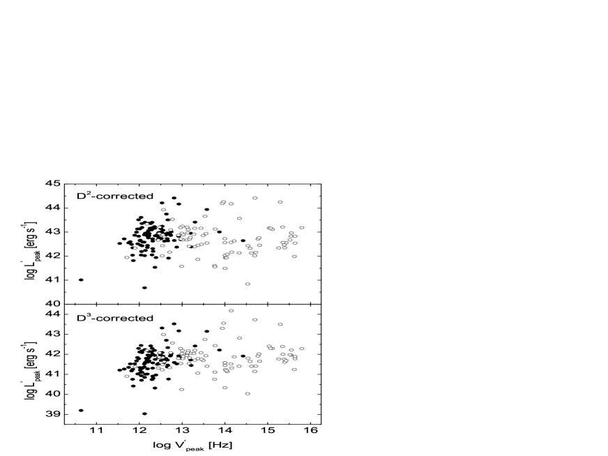
Figure 2: Doppler-corrected synchrotron peak luminosity versus Doppler-corrected synchrotron peak frequency for Fermi blazars. In the top panel, the data-points are $D^{2}$-corrected and in the bottom panel they are $D^{3}$-corrected. The meanings of different symbols are as same as Fig. 1.

3 The results

3.1 The blazar sequence

The synchrotron peak luminosity versus synchrotron peak frequency is shown in Fig. 1. A distinct “L” or “V” shape is not seen in this figure. Blazars and radio galaxies are almost located in different regions. The synchrotron peak luminosity $L_{\rm peak}$ of almost all FSRQs (BL Lacs) is larger than $L_{\rm peak}$ of FR IIs (FR Is). From Pearson correlation analysis, it is shown that for all blazars sample, there is significant anti-correlation while not significant for FSRQs; there is low anti-correlation for BL Lacs (see Table 2). In Fig. 1, there is a BL Lac (J0630.9-2406: $\log\nu_{\rm peak}=15.39$ Hz, $\log L_{\rm peak}=46.5~{}{\rm erg~{}s^{-1}}$) which is found as high $L_{\rm peak}$ and high $\nu_{\rm peak}$ blazar in Padovani, Giommi & Rau (2012).

The Doppler corrections of synchrotron peak frequency and luminosity scale as $\nu^{{}^{\prime}}=\nu/\delta$ and $L_{\rm peak}^{{}^{\prime}}=L_{\rm peak}/\delta^{\rm P}$ respectively, with $P=3+\alpha$ for a moving, isotropic source and $P=2+\alpha$ for a continuous jet ($\delta$ is Doppler factor; spectral index $\alpha=1$; Urry & Padovani 1995 and Nieppola et al. 2008). Since blazars obey $\theta_{\rm j}<1/\Gamma$, especially for Fermi blazars (Jorstad et al. 2005; Pushkarev et al. 2009; Linford et al. 2011; Wu et al. 2014), we assume $\delta\sim\Gamma$ ($\Gamma$ is estimated from radio observation or beaming factor $f_{\rm b}$). From the above relations, Doppler-corrected peak luminosity and frequency can be obtained ($D^{2}$-correction and $D^{3}$-correction stand for $P=2+\alpha$ and $P=3+\alpha$ respectively). The Doppler-corrected synchrotron peak luminosity versus Doppler-corrected synchrotron peak frequency is shown in Fig. 2. The results of Pearson correlation analysis show that for all blazar and subclass, there are not significant correlations or are significant positive correlations (both for $P=2+\alpha$ and $P=3+\alpha$; see Table 2).

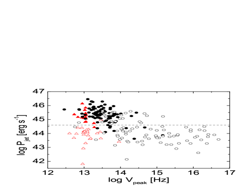
Figure 3: Jet power versus non-beaming-corrected synchrotron peak frequency. The uncertainty of jet power corresponds to 0.7 dex. The discontinuous line corresponds to $\log P_{\rm jet}\sim 44.6~{}{\rm erg~{}s^{-1}}$. The meanings of different symbols are as same as Fig. 1.

3.2 The unification of blazars and radio galaxies

Sbarrato, Padovani & Ghisellini (2014) have studied the question: “how much do we have to beam the radio luminosity of the radio galaxies to compare them with blazar?” Sbarrato, Padovani & Ghisellini (2014) beamed the radio luminosity of the radio galaxies as they were oriented as a blazar, who boosted the radio luminosity of the radio galaxies by a factor:

$$~{}~{}~{}~{}~{}~{}~{}~{}~{}~{}~{}~{}~{}~{}~{}~{}~{}(\frac{\delta_{\rm BL}}{\delta_{\rm RG}})^{3}=(\frac{1-\beta{\rm cos}\theta_{\rm RG}}{1-\beta{\rm cos}\theta_{\rm BL}})^{3},$$ (1)

where $\delta$ is the Doppler-boosting factor with apparent superluminal component velocities $\beta$. The Doppler-boosting factor is expressed as $\delta=\frac{1}{\Gamma(1-\beta{\rm cos}\theta)}$ with Lorentz factor $\Gamma=(1-\beta^{2})^{-1/2}$ and viewing angle $\theta$. Following the Sbarrato, Padovani & Ghisellini (2014), we boost the synchrotron peak frequency of radio galaxies by a factor:

$$~{}~{}~{}~{}~{}~{}~{}~{}~{}~{}~{}~{}~{}~{}~{}~{}~{}\frac{\delta_{\rm BL}}{\delta_{\rm RG}}=\frac{1-\beta{\rm cos}\theta_{\rm RG}}{1-\beta{\rm cos}\theta_{\rm BL}}.$$ (2)

We take average viewing angle $\theta_{\rm RG}\sim 40^{\circ}$ for radio galaxies and $\theta_{\rm BL}\sim 3^{\circ}$ for blazars similar to Sbarrato, Padovani & Ghisellini (2014). If we assume jets of blazar and radio galaxy are beamed with a Lorentz factor similar to a common blazar, then the Lorentz factor $\Gamma\sim 10$. If the jets of radio galaxies and blazar are characterized by a rather small Lorentz factor, then the Lorentz factor $\Gamma\sim 3$. We also estimate the factor $\frac{\delta_{\rm BL}}{\delta_{\rm RG}}$ from assuming a average Lorentz factor $\Gamma\sim 5$. The factors $\frac{\delta_{\rm BL}}{\delta_{\rm RG}}$ are 4.7, 11.6 and 37 corresponding to $\Gamma\sim$3, 5 and 10 respectively. For radio galaxies, we use $\nu_{\rm peak}^{{}^{\prime}}=(\frac{\delta_{\rm BL}}{\delta_{\rm RG}})\nu_{\rm peak}$ to beam their synchrotron peak frequency (called beam-corrected synchrotron peak frequency). The jet power versus non-beam-corrected synchrotron peak frequency and beam-corrected synchrotron peak frequency can be seen in Fig. 3 and Fig. 4 respectively. From Fig. 3 and Fig. 4, it is shown that when the synchrotron peak frequency of radio galaxy is not beam-corrected, the blazars have larger synchrotron peak frequency than radio galaxies. Therefore most of blazars do not overlap with radio galaxies. However after correcting beaming effect on peak frequency of radio galaxies, we find that most of blazars overlap with radio galaxies. From Table 2, we can get that for non-beam-corrected peak frequency, there are significant correlations between $P_{\rm jet}$ and $\nu_{\rm peak}$ for blazars$+$radio galaxies, only blazars, only BL Lacs, only FSRQs; for beam-corrected peak frequency of radio galaxies, there are significant correlations between $P_{\rm jet}$ and $\nu_{\rm peak}$ for blazars$+$radio galaxies sample, and the correlations of beam-corrected peak frequency are much stronger than the correlation of non-beam-corrected peak frequency.

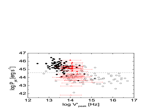
Figure 4: Jet power versus beam-corrected synchrotron peak frequency. The beam-corrected synchrotron peak frequency for radio galaxy is estimated by assuming $\Gamma\sim 5$ and viewing angle $\theta_{\rm RG}\sim 40^{\circ}$ for radio galaxies and $\theta_{\rm BL}\sim 3^{\circ}$ for blazars. The error bar is beam-corrected synchrotron peak frequency estimated by assuming Lorentz factors of 3 and 10. The uncertainty of jet power corresponds to 0.7 dex. The discontinuous line corresponds to $\log P_{\rm jet}\sim 44.6~{}{\rm erg~{}s^{-1}}$. The meanings of different symbols are as same as Fig. 1.

4 Discussions and conclusions

In order to study beaming effect on the blazar sequence and obtain jet cavity power, we consider the sample of Nemmen et al. (2012) which is large sample including beaming factor and jet cavity power but not complete sample of 2LAC. Finke (2013) studied a 2LAC sample (including blazars with unknown redshift), and used the empirical equations of Abdo et al. (2010b) to estimate the $\nu_{\rm peak}$ and $L_{\rm peak}$. Via comparing our Fig. 1 with Fig. 2 of Finke (2013), it is found that our Fig. 1 is consistent with Fig. 2 of Finke (2013). The correlation analysis of blazars (with known redshift) also supports that there is significant anti-correlation between $\nu_{\rm peak}$ and $L_{\rm peak}$ which is consistent with result of Finke (2013). In our Fig. 1, we also include radio galaxies. From Meyer et al. (2011), an “L”-shape in the $L_{\rm peak}-\nu_{\rm peak}$ plot seems to have emerged which destroys the blazar sequence. Also Meyer et al. (2011) presented the blazar envelope (FR Is and BL Lacs belong to “weak-jet” sources; FR IIs and FSRQs belong to “strong-jet” sources). However, combining blazars and radio galaxies sample, we find that our results do not have obvious the blazar envelope, especially for FR Is+BL Lacs sample. The main reason is that there are still blazars in $10^{14}{\rm Hz}<\nu_{\rm peak}<10^{15}{\rm Hz}$ interval for our sample. Our $\nu_{\rm peak}$ and $L_{\rm peak}$ are estimated from the empirical equations of Abdo et al. (2010b) who have pointed out that their method assumed that the optical and X-ray fluxes are not contaminated by thermal emission from the disk or accretion. In blazars where thermal flux components are not negligible (this should probably occur more frequently in low radio luminosity sources) the method may lead to a significant overestimation of the position of $\nu_{\rm peak}$. From Finke (2013), the following factors can have effect on estimating $\nu_{\rm peak}$ and $L_{\rm peak}$: the measurement error on determining $\nu_{\rm peak}$ and $L_{\rm peak}$, the fitting function of SED and variability. Finke (2013) have pointed out that the results in $L_{\rm peak}$ versus $\nu_{\rm peak}$ plot are probably not accurate for individual sources, whereas the overall trend still is present even for large errors. From Equations (1), (3) and (4) of Abdo et al. (2010b), it is in turn got that $\alpha_{\rm ro}\propto-logf_{\rm r}$, $\log\nu_{\rm peak}\propto\log f_{\rm r}$, and $\log L_{\rm peak}\propto\log f_{\rm r}$ ($f_{\rm r}$ is radio flux, $\alpha_{\rm ro}$ is broadband spectral slopes between radio and optics). So even if the correlation between $L_{\rm peak}$ and $\nu_{\rm peak}$ is dominated due to both dependence on radio flux, the correlation should be positive but not anti-correlation. In addition, when accounting for the common dependence on radio flux (if any), we use Pearson partial correlation analysis to analyze the correlation between $L_{\rm peak}$ and $\nu_{\rm peak}$ for all blazars. The result shows that the significant correlation still exist ($r=-0.47,P=3\times 10^{-11}$). In our sample, there is a BL Lac which is found as high $L_{\rm peak}$ and high $\nu_{\rm peak}$ blazar in Padovani, Giommi & Rau (2012). Ghisellini et al. (2012) have found that the four high $L_{\rm peak}$ and high $\nu_{peak}$ sources from Padovani, Giommi & Rau (2012) do not have excessively large $\gamma$-ray luminosity or excessively small $\gamma$-ray photon index. However, if the high $L_{\rm peak}$ and high $\nu_{\rm peak}$ blazars indeed exist, the blazars sequence based on $L_{\rm peak}-\nu_{\rm peak}$ will be destroyed.

Another attention of the blazars sequence is beaming effect on $L_{\rm peak}$ and $\nu_{\rm peak}$. Then the Doppler factor or bulk Lorentz factor should be obtained. The variability Doppler factor was derived from the associated variability brightness temperature of total radio flux density flares with the intrinsic value of brightness temperature, and the bulk Lorentz factor from apparent super-luminal component velocities and variability Doppler factor (Hovatta et al. 2009). For the blazars without without $\Gamma_{\rm var}$ obtained from Pushkarev et al. (2009), Nemmen et al. (2012) used $\gamma$-ray luminosity to estimate beaming factor with 3.6$\sigma$ significant level. For blazars with variability bulk Lorentz factor available, the relative uncertainty in $\Gamma$ is 0.3 and the relative uncertainty in $\Gamma$ estimated from the $L_{\rm\gamma}-f_{\rm b}$ relationship is 0.7 (Nemmen et al. 2012). Furthermore, we assume $\Gamma\sim\delta$ which is reasonable because $\theta_{\rm j}<1/\Gamma$ for blazars, especially for Fermi blazars with a larger beaming factor and smaller $\theta_{\rm j}$ (Jorstad et al. 2005; Pushkarev et al. 2009; Linford et al. 2011; Wu et al. 2014). It is noted that the above estimating $\delta$ is probably not accurate for individual sources. From Fig. 2 and Table 2, we find that after being Doppler-corrected, for all blazar and subclass, the correlations between $L_{\rm peak}$ and $\nu_{\rm peak}$ are not significant or become significant positive correlations, i.e. the anti-correction between $L_{\rm peak}$ and $\nu_{\rm peak}$ disappears, which is consistent with result of Nieppola et al. (2008).

Through studying the correlation between jet power and the synchrotron peak frequency, it is found that there is significant anti-correlation between $P_{\rm jet}$ and $\nu_{\rm peak}$ for Fermi blazars, which supports the blazar sequence, i.e. a stronger radiative cooling for higher jet power sources results in smaller energies of the electrons emitting at the peaks. In addition, the results also imply the BL Lacs - FSRQs divide. From Ghisellini et al. (2009, 2011, 2015), Sbarrato et al. (2012), Sbarrato, Padovani & Ghisellini (2014) and Xiong & Zhang (2014), it is got that $P_{\rm jet}\sim L_{\rm disk}$ and the physical distinction between BL Lacs and FSRQs is $L_{\rm BLR}/L_{\rm Edd}\sim 10^{-3}$. Based on result of Xiong & Zhang (2014), the average black hole mass of Fermi blazars is $\sim 10^{8.5}{\rm M_{\odot}}$. Then the jet power of BL Lacs and FSRQs divide corresponds to $\log P_{\rm jet}\sim 44.6~{}{\rm erg~{}s^{-1}}(L_{\rm Edd}=1.3\times 10^{38}(\rm\frac{M}{M_{\odot}}){\rm erg~{}s^{-1}},L_{\rm disk}\approx 10L_{\rm BLR}$, $M\sim 10^{8.5}{\rm M_{\odot}}$). The Fig. 3 and Fig. 4 present the divide line which also supports the physical distinction. The BL Lacs with $\log P_{\rm jet}>44.6~{}{\rm erg~{}s^{-1}}$ (i.e. $L_{\rm BLR}/L_{\rm Edd}>10^{-3}$) can be considered as transition sources (see Ghisellini et al. 2011). Moreover, the BL Lac which is found as high $L_{\rm peak}$ and high $\nu_{\rm peak}$ blazar in Padovani, Giommi & Rau (2012) does not have high jet cavity power ($\log P_{\rm jet}=43.2~{}{\rm erg~{}s^{-1}}$). A possible explanation is that the high $L_{\rm peak}$ and high $\nu_{\rm peak}$ blazar is resulted from beaming effect while the blazar virtually is low power source. Ghisellini et al. (2009) have studied the $\gamma$-ray luminosity versus $\gamma$-ray photon index (a proxy for inverse Compton peak frequency), and proposed the Fermi blazars divide. We should note that there is beaming effect on $\gamma$-ray luminosity while not on jet power estimated from extended radio emission.

Next, we will discuss the unification of blazars and radio galaxies. The Fig. 3 and Fig. 4 show that when the synchrotron peak frequency of radio galaxy is not beam-corrected, most of blazars do not overlap with radio galaxies (especially for FR Is and BL Lacs), while after being beam-corrected peak frequency for radio galaxies, most of blazars overlap with radio galaxies. Nieppola et al. (2008) have found the dependence between Doppler factor and $\nu_{\rm peak}$ for blazars. So the $\nu_{\rm peak}$ should be Doppler-corrected or ruled out the influence of beaming effect. However, it is not possible to derive the specific Lorentz factor/Doppler factor for each source, especially for radio galaxies. In this paper, we adopt the method of Sbarrato, Padovani & Ghisellini (2014). Making use of different Lorentz factor, we analyze the correlations between jet power and beam-corrected peak frequency for blazars$+$radio galaxies sample. From Table 2, we can get that after being beam-corrected peak frequency of radio galaxies, there are significant correlations between jet power and peak frequency for blazars$+$radio galaxies sample, and the correlations of beam-corrected peak frequency are much stronger than the correlation of non-beam-corrected peak frequency. When beaming-corrected peak frequency, the assuming Lorentz factors are reasonable. For blazars, the $\Gamma\sim$3, 5 and 10 are possible (see Sbarrato, Padovani & Ghisellini (2014) for detail). Giovannini et al. (2001) studied a complete sample of radio galaxies, and estimated that relativistic jets with Lorentz factor in the range 3 - 10 are present in high and low power radio sources. Now, we explain how to associate the correlations between jet power and beam-corrected $\nu_{\rm peak}^{{}^{\prime}}$ with the unification of blazars and radio galaxies. Urry & Padovani (1995) have explained that the radio extended luminosity of FR IIs (FR Is) and FSRQs (BL Lacs) should be comparable. Our jet cavity power is estimated from radio extended luminosity. Then the jet power between FR IIs (FR Is) and FSRQs (BL Lacs) should be comparable. In addition, as discussed in the previous paragraph, the division between FSRQs and BL Lacs is $\log P_{\rm jet}\sim 44.6~{}{\rm erg~{}s^{-1}}$ or $L_{\rm d}/L_{\rm Edd}\sim 10^{-2}$. According to the two-dimensional optical-radio luminosity correlation from Owen & Ledlow (1994), Ghisellini & Celotti (2001) found that the division between FR IIs and FR Is is $P_{\rm jet}\sim 0.015L_{\rm Edd}$. If the radio galaxies have similar average black hole mass with blazars, then the division between FR IIs and FR Is also is $\log P_{\rm jet}\sim 44.6~{}{\rm erg~{}s^{-1}}$. From Fig. 3 and Fig. 4, it is seen that the line of $\log P_{\rm jet}\sim 44.6~{}{\rm erg~{}s^{-1}}$ also can separate FR Is from FR IIs. Abdo et al. (2010b) subdivided blazars based on the $\nu_{\rm peak}$ (low/intermediate/high-synchrotron-peaked blazar). Almost all FSRQs are low-synchrotron-peaked blazar and BL Lacs include low/intermediate/high-synchrotron-peaked blazar. Based on unified scheme, after being beam-corrected, the $\nu_{\rm peak}$ should be comparable between FR IIs (FR Is) and FSRQs (BL Lacs) because the differences between FR IIs (FR Is) and FSRQs (BL Lacs) mainly rely on jet angle to the line of sight. Therefore based on above discussion, in $P_{\rm jet}-\nu_{\rm peak}^{{}^{\prime}}$ plot, blazars

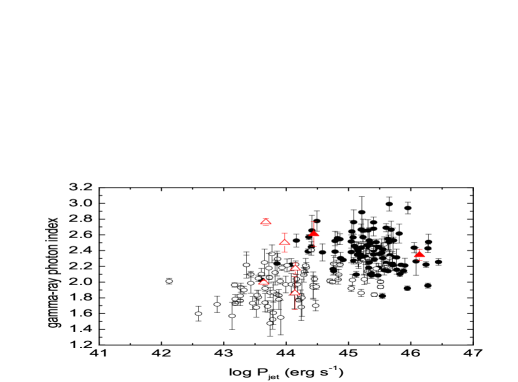
Figure 5: $\gamma$-ray photon index versus jet power. The uncertainty of jet power corresponds to 0.7 dex. The meanings of different symbols are as same as Fig. 1.

and radio galaxies should have a similar correlation, i.e. the blazars and radio galaxies can be unified from the correlation between jet power and beam-corrected peak frequency. At present, since only there are limited radio galaxies with precise Lorentz factor estimated from observation, it is hard to accurately estimate beam-corrected peak frequency for individual sources. In order to test whether assuming Lorentz factors bring in remarkable effect on the overall trend which results in spurious correlation, We also analyze the correlation between jet power and $\gamma$-ray photon index for Fermi blazar and radio galaxie because $\gamma$-ray photon index is free of beaming effect and $L_{\rm\gamma}$ versus $\gamma$-ray photon index has been used to support the blazar sequence. If for blazars and radio galaxies, the correlations between jet power and $\gamma$-ray photon index still exist and are consist with the correlation between $P_{\rm jet}$ and beam-corrected $\nu_{\rm peak}^{{}^{\prime}}$, then it is clarified that our assuming Lorentz factors do not bring in remarkable effect on the overall trend. From Fig. 5 (FR Is: 3C 78, 3C 84, M87, Cen A, NGC 6251; FR IIs: 3C 380, 3C 111), the correlations between jet power and $\gamma$-ray photon index still exist and support the blazar sequence (higher jet power - softer photon index). In the $\gamma$-ray photon index versus jet power plot, FR IIs overlap with FSRQs and most of FR Is with BL Lacs, which support the unification of blazars and radio galaxies, similar to the correlation between $P_{\rm jet}$ and beam-corrected $\nu_{\rm peak}^{{}^{\prime}}$. Therefore, the assuming Lorentz factors do not bring in remarkable effect on the overall trend.

Table 1: The Fermi blazar sample.

2FGL name	Type	$Z^{\rm(a)}$	$\log P_{\rm jet}^{\rm(b)}$	$\log f_{\rm b}^{\rm(c)}$	$F_{\rm R}^{\rm(d)}$	$\log\nu_{\rm peak}^{\rm(e)}$	$\log L_{\rm peak}^{\rm(e)}$
J0050.6-0929	BLL	0.634	44.31	-2.08	1920	14.83	46.86
J0108.6+0135	FSRQ	2.099	46.46	-3.21$\ast$	3400	13.10	47.08
J0112.1+2245	BLL	0.265	43.75	-2.27	327	14.98	45.52
J0112.8+3208	FSRQ	0.603	45.21	-2.52	405	13.15	45.37
J0116.0-1134	FSRQ	0.67	45.46	-2.43	1900	13.30	46.13
J0120.4-2700	BLL	0.559	45.06	-2.45	1035	13.99	46.10
J0132.8-1654	FSRQ	1.02	45.22	-2.65	1584	13.73	46.60
J0136.9+4751	FSRQ	0.859	44.78	-2.62$\ast$	3150	13.69	46.73
J0137.6-2430	FSRQ	0.838	45.57	-2.45	1558	13.58	46.37
J0141.5-0928	BLL	0.733	45.08	-2.41	1200	14.06	46.41
J0205.3-1657	FSRQ	1.739	45.42	-2.79	1400	13.46	46.79

(a) redshift directly collected from NED. (b) jet power estimated by cavity power in unit of ${\rm erg~{}s^{-1}}$. (c) beaming factor $f_{\rm b}=1-{\rm cos}(1/\Gamma)$. values with a “ $\ast$ ” represent that they are directly from radio observation. (d) total radio 5 GHz flux in mJy. (e) rest-frame synchrotron peak frequency and luminosity in Hz and ${\rm erg~{}s^{-1}}$.

(f) This table is published in its entirety in the electronic edition. A portion is shown here for guidance.

Table 2: The results of correlation analysis.

Sample	$L_{\rm peak}$ versus $\nu_{\rm peak}^{\rm(a)}$	$L_{\rm peak}^{\rm D2}$ versus $\nu_{\rm peak}^{\rm D(b)}$	$L_{\rm peak}^{\rm D3}$ versus $\nu_{\rm peak}^{\rm D(c)}$	$P_{\rm jet}$ versus $\nu_{\rm peak}^{\rm(e)}$
	$r^{(f)}$           $P^{(f)}$	$r$          $P$	$r$           $P$	$r$           $P$
Blazars	-0.5     $4.2\times 10^{-13}$	0.009         0.9	0.26     $3\times 10^{-4}$	-0.69   $3\times 10^{-27}$
BL Lacs	-0.24    0.02	-0.03         0.8	0.12        0.26	-0.45   $1.7\times 10^{-5}$
FSRQs	-0.18    0.07	0.33     $1\times 10^{-3}$	0.46   $1.5\times 10^{-6}$	-0.52   $4.8\times 10^{-8}$
Sample	$P_{\rm jet}$ versus $\nu_{\rm peak}^{\rm D(d)}$ ($\Gamma\sim 3$)	$P_{\rm jet}$ versus $\nu_{\rm peak}^{\rm D(d)}$ ($\Gamma\sim 5$)	$P_{\rm jet}$ versus $\nu_{\rm peak}^{\rm D(d)}$ ($\Gamma\sim 10$)	$P_{\rm jet}$ versus $\nu_{\rm peak}^{\rm(e)}$
Blazars+RG	-0.59     $2.6\times 10^{-22}$	-0.62    $1.2\times 10^{-25}$	-0.64    $2.1\times 10^{-27}$	-0.50   $2.6\times 10^{-15}$

(a) Synchrotron peak luminosity versus synchrotron peak frequency. (b) Doppler-corrected synchrotron peak luminosity versus Doppler-corrected synchrotron peak frequency ($D^{2}$-corrected). (c) Doppler-corrected synchrotron peak luminosity versus Doppler-corrected synchrotron peak frequency ($D^{3}$-corrected). (d) jet power versus beam-corrected synchrotron peak frequency from assuming $\Gamma\sim$3, 5 and 10. (e) jet power versus non-beam-corrected synchrotron peak frequency.

(f) The $r$ is the Pearson correlation coefficient; $P$ is the chance probability.

References

- Abdo et al. (2010b) Abdo A.A., Ackermann M., Ajello M. et al., 2010a, ApJ, 715, 429
- Abdo et al. (2010c) Abdo A.A., Ackermann M., Agudo I. et al., 2010b, ApJ, 716, 30
- Ackermann et al. (2011a) Ackermann M., Ajello M., Allafort A. et al., 2011, ApJ, 743, 171
- Angel (1980) Anton S. & Browne I.W.A., 2005, MNRAS, 356, 225
- Caccianiga (2004) Caccianiga A. & Marcha M.J.M., 2004, MNRAS, 348, 937
- Cavaliere & D’Elia (2002) Cavaliere A. & D’Elia V., 2002, ApJ, 571, 226
- Chen et al. (2011) Chen L. & Bai J.M., 2011, ApJ, 735, 108
- Chen et al. (2011) Chen L., 2014, ApJ, 788, 179
- Fan (1998) Fanaroff B.L. & Riley J.M., 1974, MNRAS, 167, 31
- Finke (1994) Finke J.D., 2013, ApJ, 763, 134
- Fossati et al. (1998) Fossati G., Maraschi L., Celotti A. et al., 1998, MNRAS, 299, 433
- Francis et al. (1991) Georganopoulos M., Kirk J.G. & Mastichiadis A., 2001, in ASP Conf. Ser. 227, Blazar Demographics and Physics, ed. P. Padovani & C. Megan Urry (San Francisco, CA: ASP), 116
- Ghisellini (1998) Ghisellini G., Celotti A., Fossati G. et al., 1998, MNRAS, 301, 451
- Ghisellini (2001) Ghisellini G. & Celotti A., 2001, A&A, 379, 1
- Ghisellini & Tavecchio (2008) Ghisellini G. & Tavecchio F., 2008, MNRAS, 387, 1669
- Ghisellini et al. (2009a) Ghisellini G., Maraschi L. & Tavecchio F., 2009, MNRAS, 396, 105
- Ghisellini et al. (2010) Ghisellini G., Tavecchio F., Foschini L., Ghirlanda G., Maraschi L. & Celotti A., 2010, MNRAS, 402, 497
- Ghisellini et al. (2011) Ghisellini G., Tavecchio F., Foschini L. & Ghirlanda G., 2011, MNRAS, 414, 2674
- Ghisellini et al. (2011) Ghisellini G., Tavecchio F., Foschini L. et al. 2012, MNRAS, 425, 1371
- Ghisellini et al. (2014) Ghisellini G., Tavecchio F., Maraschi L., Celotti A. & Sbarrato T., 2014, Nature, 515, 376
- Ghisellini et al. (2015) Ghisellini G. & Tavecchio F., 2015, MNRAS, 448, 1060
- Giommi et al. (1999) Giommi P., Menna M.T. & Padovani P., 1999, MNRAS, 310, 465
- Giommi et al. (2012) Giommi P., Padovani P., Polenta G., Turriziani S., D’Elia V. & Piranomonte S., 2012, MNRAS, 420, 2899
- Giommi et al. (2013) Giommi P., Padovani P. & Polenta G., 2013, MNRAS, 431, 1914
- Giovannini et al. (2001) Giovannini G., Cotton W.D., Feretti L. Lara L. & Venturi T., 2001, ApJ, 552, 508
- Gu et al. (2009) Gu M., Cao X. & Jiang D.R., 2009, MNRAS, 396, 984
- Gu et al. (2009) Hovatta T., Valtaoja E., Tornikoski M. & Lahteenmaki A., 2009, A&A, 494, 527
- Jorstad et al. (2001) Jorstad S.G., Marscher A.P., Mattox J.R., Wehrle A.E., Bloom S.D. & Yurchenko A.V., 2001, ApJS, 134, 181
- Ledlow (1994) Ledlow M.J. & Owen F.N., 1994, in The Physics of Active Galaxies, ASP Conf. Ser. 54, ed. G.V. Bicknell, M.A. Dopita, & P.J. Quinn, 319
- Linford et al. (2011) Linford J.D., Taylor G.B., Romani R. et al., 2011, ApJ, 726, 16
- Maraschi et al. (2008) Maraschi L., Foschini L., Ghisellini G., Tavecchio F. & Sambruna R.M., 2008, MNRAS, 391, 1981
- Maraschi et al. (1992) Maraschi L. & Tavecchio F., 2003, ApJ, 593, 667
- Meyer et al. (2011) Meyer E.T., Fossati G., Georganopoulos M. & Lister M.L., 2011, ApJ, 740, 98
- Nemmen et al. (2001) Nemmen R.S., Georganopoulos M., Guiriec S., Meyer E.T., Gehrels N., & Sambruna R.M., 2012, Science, 338, 1445
- Nieppola et al. (2006) Nieppola E., Tornikoski M. & Valtaoja E., 2006, A&A, 445, 441
- Nieppola et al. (2008) Nieppola E., Valtaoja E., Tornikoski M., Hovatta T. & Kotiranta M., 2008, A&A, 488, 867
- Padovani (2003) Padovani P., Perlman E.S., Landt H., Giommi P. & Perri M., 2003, ApJ, 588, 128
- Padovani (2007) Padovani P., 2007, Ap&SS, 309, 63
- Padovani (2007) Padovani P., Giommi P. & Rau A., 2012, MNRAS, 422, 48
- Pushkarev (2009) Pushkarev A.B., Kovalev Y.Y., Lister M.L. & Savolainen T., 2009, A&A, 507, 33
- Sambruna et al. (2010) Sambruna R.M. et al., 2010, ApJ, 710, 24
- Sbarrato et al. (2012) Sbarrato T., Ghisellini G., Maraschi L. & Colpi M., 2012, MNRAS, 421, 1764
- Sbarrato et al. (2014) Sbarrato T., Padovani P. & Ghisellini G., 2014, MNRAS, 445, 81
- Urry & Padovani (1995) Urry C.M. & Padovani P., 1995, PASP, 107, 803
- Wu (2007) Wu Z.Z., Jiang D.R., Gu M.F. & Liu, Y., 2007, A&A, 466, 63
- Wu (2014) Wu Z.Z., Jiang D.R. & Gu M.F., 2014, A&A, 562, 64
- Xie et al. (2007) Xie G.Z., Dai H. & Zhou S.B., 2007, AJ, 134, 1464
- Xiong (2014) Xiong D.R. & Zhang X., 2014, MNRAS, 441, 3375
- Zirbel (1995) Zirbel E.L. & Baum S.A., 1995, ApJ, 448, 521